Consistent and Efficient Pricing of SPX and VIX Options under Multiscale Stochastic Volatility

Abstract

This study provides a consistent and efficient pricing method for both Standard & Poor’s 500 Index (SPX) options and the Chicago Board Options Exchange’s Volatility Index (VIX) options under a multiscale stochastic volatility model. To capture the multiscale volatility of the financial market, our model adds a fast scale factor to the well-known Heston volatility and we derive approximate analytic pricing formulas for the options under the model. The analytic tractability can greatly improve the efficiency of calibration compared to fitting procedures with the finite difference method or Monte Carlo simulation. Our experiment using options data from 2016 to 2018 shows that the model reduces the errors on the training sets of the SPX and VIX options by 9.9% and 13.2%, respectively, and decreases the errors on the test sets of the SPX and VIX options by 13.0% and 16.5%, respectively, compared to the single-scale model of Heston. The error reduction is possible because the additional factor reflects short-term impacts on the market, which is difficult to achieve with only one factor. It highlights the necessity of modeling multiscale volatility.

1 Introduction

Volatility in the financial market is one of the most important measures for investors. The Volatility Index (VIX) of the Chicago Board Options Exchange (CBOE) was introduced as a measure to capture the volatility of the Standard & Poor’s 500 Index (SPX) in 1993. The VIX was revised to be independent of any model in 2003. After the revision, it is calculated using SPX option prices and the SPX over the next 30 calendar-day period. Since the introduction of the VIX, the index has become a standard gauge of market fear, because the VIX and the SPX are negatively correlated. In addition, VIX options also have received a lot of attention as the popularity of the VIX has grown, and this interest in the derivatives has led to the development of an appropriate pricing method for them.

It is noteworthy that many researchers have invented pricing methods for VIX options under the models originally proposed to price SPX options. This may be because an arbitrage relationship exists between the SPX option market and the VIX option market. In the early research period for VIX options, there were the studies to derive pricing formulas for VIX options under several one-factor affine jump diffusion (AJD) models; Lin and Chang (2009), Lian and Zhu (2013), Lin and Chang (2010), Cheng et al. (2012) and Cont and Kokholm (2013). As it is widely known, the one-factor AJD model has a special structure from a mathematical standpoint, so they often give a pricing formula for a derivative for SPX options as well as VIX options (refer Duffie et al., 2000). It is highly desirable in the sense that they make it possible to evaluate the SPX options and the VIX options without arbitrage. However, it is recognized that the one-factor AJD models have a variety of fundamental limitations. Above all, the models cannot accommodate the multiscale property of volatility, which highlights the necessity of multi-factor affine diffusion models. Jumps are usually excluded in the models, but it is frequently stated that the models are superior to the one-factor AJD models in literature such as Kaeck and Alexander (2012).

In this light, Gatheral (2008) proposed the double-mean-reverting (DMR) Heston model to capture the multiscales of volatility. But it does not provide any pricing formula and depends on the Monte-Carlo simulation totally for a pricing and a calibration. Although the simulation method has been greatly improved in Bayer et al. (2013), the model still fails to suggest a viable solution to a calibration using a large number of option prices. On the other hand, Fouque and Saporito (2018) proposed the Heston stochastic vol-of-vol model (Heston SVV model) with fast and slow time scales to reflect skews in both the SPX data and VIX data, and derived approximation solutions for the prices of options on the SPX and VIX, respectively. Moreover, it showed that the Heston SVV model calibrated jointly to real market data for the SPX and VIX fits to the data very well. Their solutions, however, cannot be also computed within a short period of time. Interestingly, Huh et al. (2018) obtained an approximate quasi-closed formula for VIX options under the DMR Heston model, and furthermore, it confirmed with real market data that the calibration result utilizing the approximate solution is analogous to the case using simulation methods. But the approach can be applied to pricing VIX options only.

Our novel model is the first multi-factor affine diffusion model to give practically feasible pricing formulas for both SPX options and VIX options. To be concrete, we propose a new two-factor affine diffusion model, and induce approximate quasi-closed formulas for both the options based upon the perturbation theory. The analytic tractability greatly improve the efficiency of calibration. As a result, we could achieve satisfactory calibration results with long-term data for the SPX and VIX from 2016 to 2018, consisting of hundreds of thousands of options.

The remainder of the paper is organized as follows. We introduce a new two-factor model with multiscale volatility to jointly price VIX options and SPX options in Section 2. We derive the analytic pricing formulas of SPX options and VIX options under the proposed model using asymptotic methods in Section 3. We present calibration with real options data for the SPX and VIX in Section 4. We provide concluding remarks in Section 5.

2 A new two-factor multiscale stochastic volatility model

Before introducing our model, we briefly review the double Heston model of Christoffersen et al. (2009). The model was originally devised to reflect stochastic correlation as well as stochastic volatility. The improvement is achievable because the model has two factors. By contrast, the Heston model cannot capture stochastic correlation because it has only one factor. The double Heston model, however, cannot capture the multiscale characteristics of a market, because it was not designed for this purpose (see Gallant et al., 1999; Chernov et al., 2003). Thus, the model needs to be extended to depict well-separated time scales. More importantly, the model provides an analytic formula for VIX options, which requires heavy computation for a double integral. In particular, when practitioners want to fit the model to prices for both SPX options and VIX options consistently within a limited time, the time cost raises a severe problem.

To overcome these limitations of the double Heston model, we propose a two-factor multiscale stochastic volatility model, which is given by the following stochastic differential equations:

$$dX_{t} =rX_{t}dt+\sqrt{Y_{t}}X_{t}dW_{t}^{X,1}+\sqrt{Z_{t}}X_{t}dW_{t}^{X,2},$$

$$dY_{t} =\frac{1}{\epsilon}\left(Z_{t}-Y_{t}\right)dt+\frac{\sqrt{2}\nu}{\sqrt{\epsilon}}\sqrt{Y_{t}}dW_{t}^{Y},$$ (1)

$$dZ_{t} =\kappa\left(\theta-Z_{t}\right)dt+\sigma\sqrt{Z_{t}}dW_{t}^{Z}$$

for $0<\epsilon\ll 1$ under a risk-neutral measure $\mathcal{Q}$, where $r$ is the risk-free rate, and $\kappa\ll 1/\epsilon$ is assumed. The correlation structure of our model is

$$dW_{t}^{X,1}dW_{t}^{Y}=\eta dt,\quad dW_{t}^{X,2}dW_{t}^{Z}=\rho dt,$$

$$dW_{t}^{X,1}dW_{t}^{Z}=dW_{t}^{X,2}dW_{t}^{Y}=dW_{t}^{X,1}dW_{t}^{X,2}=dW_{t}^{Y}dW_{t}^{Z}=0.$$

It should be noted that $Y_{t}$ rapidly reverts to $Z_{t}$ under our model, which is a major difference with the double Heston model. Because the time scales are clearly separated due to condition $\kappa\ll 1/\epsilon$, the short-term variance $ourY_{t}+Z_{t}$ rapidly reverts to mid-term variance $2Z_{t}$, and $2Z_{t}$ regresses to long-term variance $2\theta$ at a relatively slow rate. On the other hand, one can consider that our model is obtained by adding a fast mean-reverting factor to Heston’s volatility or otherwise by modifying the double Heston model to express the well-separated time scales.

3 Pricing SPX and VIX options

3.1 An approximate analytic formula for SPX options

By the risk-neutral pricing principle, the price $P_{s}^{\epsilon}$ for an SPX call option with strike $K$ and maturity $T$ at time $t$ is

$$P_{s}^{\epsilon}\left(t,x,y,z\right)=e^{-r\left(T-t\right)}{\rm E}_{x,y,z}^{\mathcal{Q}}\left[\left(X_{T}-K\right)^{+}\right],$$ (2)

where $\left(X_{t},Y_{t},Z_{t}\right)=\left(x,y,z\right)$. Applying the Feynman–Kac theorem to our model (1), it can be shown that $P_{s}^{\epsilon}$ should satisfy the following partial differential equation (PDE):

$$\left(\frac{1}{\epsilon}\mathcal{L}_{s,0}+\frac{1}{\sqrt{\epsilon}}\mathcal{L}_{s,1}+\mathcal{L}_{s,2}\right)P_{s}^{\epsilon}\left(t,x,y,z\right)=0,$$

where

$$\mathcal{L}_{s,0} = \left(z-y\right)\partial_{y}+\nu^{2}y\partial_{yy}^{2},$$

$$\mathcal{L}_{s,1} = \sqrt{2}\eta\nu xy\partial_{xy}^{2},$$ (3)

$$\mathcal{L}_{s,2} = \partial_{t}+rx\partial_{x}+\kappa\left(\theta-z\right)\partial_{z}+\frac{1}{2}x^{2}\left(y+z\right)\partial_{xx}^{2}+\frac{1}{2}\sigma^{2}z\partial_{zz}^{2}+\rho\sigma xz\partial_{xz}^{2}-r\cdot$$

with the final condition $P_{s}^{\epsilon}\left(T,x,y,z\right)=\left(x-K\right)^{+}$. Deriving an analytic solution for this PDE would be desirable; however, we confirm that the solution cannot be easily induced.

Thus, we attempt to obtain an approximate solution for $P_{s}^{\epsilon}$ based on asymptotic methods (refer to Fouque et al. (2011)). Let us expand $P_{s}^{\epsilon}$ with respect to $\sqrt{\epsilon}$, that is, $P_{s}^{\epsilon}=P_{s,0}+\sqrt{\epsilon}P_{s,1}+\epsilon P_{s,2}+\cdots.$ We wish to approximate $P_{s}^{\epsilon}$ to the sum of the leading term $P_{s,0}$ and the first non-zero correction term $P_{s,1}$. To do this, we show that $P_{s,0}$ and $P_{s,1}$ follow the following PDEs independent of $y$:

• leading term $P_{s,0}$

  $$\left\langle\mathcal{L}_{s,2}\right\rangle P_{s,0}=0,$$

  $$P_{s,0}\left(T,x,z\right)=\left(x-K\right)^{+},$$ (4)

• first non-zero correction term $P_{s,1}$

  $$\left\langle\mathcal{L}_{s,2}\right\rangle P_{s,1}=W_{3}^{\epsilon}zx\partial_{x}\left(x^{2}\partial_{xx}\right)P_{s,0},$$

  $$P_{s,1}\left(T,x,z\right)=0,$$ (5)

where

$$\left\langle\mathcal{L}_{s,2}\right\rangle=\partial_{t}+rx\partial_{x}+\kappa\left(\theta-z\right)\partial_{z}+x^{2}z\partial_{xx}^{2}+\frac{1}{2}\sigma^{2}z\partial_{zz}^{2}+\rho\sigma xz\partial_{xz}^{2}-r,$$

$$W_{3}^{\epsilon}=-\frac{1}{\sqrt{2}}\eta\nu\sqrt{\epsilon}.$$

If setting $2z=\xi$, the operator $\left\langle\mathcal{L}_{s,2}\right\rangle$ changes to

$$\mathcal{L}_{H}=\partial_{t}+rx\partial_{x}+\kappa\left(2\theta-\xi\right)\partial_{\xi}+\frac{1}{2}x^{2}\xi\partial_{xx}^{2}+\frac{1}{2}\left(\sqrt{2}\sigma\right)^{2}\xi\partial_{\xi\xi}^{2}+\left(\frac{1}{\sqrt{2}}\rho\right)\left(\sqrt{2}\sigma\right)x\xi\partial_{x\xi}^{2}-r.$$

The resulting operator $\mathcal{L}_{H}$ can be then regarded as that generated from the Heston model whose parameters are the mean-reverting rate $\kappa$, the long-term variance level $2\theta$, the volatility of volatility $\sqrt{2}\sigma$, and the leverage correlation $\rho/\sqrt{2}$.

The analytic solutions for the PDEs can be obtained by exploiting the analytical tractability of affine models fully. In fact, the key idea for the derivation of the solutions is strongly motivated by the work of Fouque and Lorig (2011). However, under their model, the solutions for SPX options are involved in triple integrals requiring overly large computational resources. By contrast, it is proved that our solutions are all involved in single integrals. More importantly, they give a solution only for SPX options, but we provide consistent solutions for both SPX options and VIX options. The expressions for $P_{s,0}$ and $P_{s,1}$ are summarized in the following theorem.

Theorem 1.

The price $P_{s}^{\epsilon}$ in (2) can be approximated with an accuracy of order $O\left(\epsilon\right)$, that is,

$$\left|P_{s}^{\epsilon}-\left(P_{s,0}+P_{s,1}\right)\right|<C\epsilon$$

for some $C>0$. Furthermore, $P_{s,0}$ and $P_{s,1}$ have the following forms:

$$P_{s,0}\left(t,x,z\right)=\frac{e^{-r\tau}}{2\pi}\int e^{-ikq}\hat{G}\left(\tau,k,2z\right)\hat{h}\left(k\right)dk,$$

$$P_{s,1}\left(t,x,z\right)=\frac{e^{-r\tau}}{2\pi}\int e^{-ikq}b\left(k\right)\left(\kappa\theta\hat{f}_{0}\left(\tau,k\right)+2z\hat{f}_{1}\left(\tau,k\right)\right)\hat{G}\left(\tau,k,2z\right)\hat{h}\left(k\right)dk,$$

where $\tau=T-t$, $q=r\tau+\log x$,

$$\hat{G}\left(\tau,k,y\right) =e^{C\left(\tau,k\right)+yD\left(\tau,k\right)},$$

$$\hat{h}\left(k\right) =\frac{K^{1+ik}}{ik-k^{2}},$$

$$\hat{f}_{0}\left(\tau,k\right) =\frac{2\tau d\left(k\right)g\left(k\right)+g^{2}\left(k\right)-1}{d^{2}\left(k\right)g\left(k\right)\left(g\left(k\right)e^{\tau d\left(k\right)}-1\right)}+\frac{\tau d\left(k\right)g\left(k\right)-g\left(k\right)-1}{d^{2}\left(k\right)g\left(k\right)},$$

$$\hat{f}_{1}\left(\tau,k\right) =\frac{e^{\tau d\left(k\right)}\left(g\left(k\right)^{2}\left(e^{\tau d\left(k\right)}-1\right)-2\tau d\left(k\right)g\left(k\right)+1\right)-1}{d\left(k\right)\left(g\left(k\right)e^{\tau d\left(k\right)}-1\right)^{2}},$$

and

$$C\left(\tau,k\right) =\frac{\kappa\theta}{\sigma^{2}}\left(\left(\kappa+\rho ik\sigma-d\left(k\right)\right)\tau-2\log\left(\frac{e^{-\tau d\left(k\right)}-g\left(k\right)}{1-e^{-\tau d\left(k\right)}g\left(k\right)}\right)\right),$$

$$D\left(\tau,k\right) =\frac{\kappa+\rho ik\sigma+d\left(k\right)}{2\sigma^{2}}\left(\frac{e^{-\tau d\left(k\right)}-1}{e^{-\tau d\left(k\right)}-g\left(k\right)}\right),$$

$$b\left(k\right) =-\frac{1}{2}W_{3}^{\epsilon}\left(ik^{3}+k^{2}\right),$$

$$d\left(k\right) =\sqrt{2\sigma^{2}\left(k^{2}-ik\right)+\left(\kappa+\rho ik\sigma\right)^{2}},$$

$$g\left(k\right) =\frac{\kappa+\rho ik\sigma+d\left(k\right)}{\kappa+\rho ik\sigma-d\left(k\right)}.$$

Proof.

The detailed proof is in A. ∎

3.2 Relationship between the VIX and our model

Before proceeding, we show the relationship between the VIX and our model. Because the VIX at time $t$, ${\rm VIX}_{t}^{\epsilon}$, is the square root of an integration of spot variance from $t$ to $t+\tau_{0}$ $\left(\tau_{0}:=30/365\right)$, based on Carr and Madan (1998), the relationship can be given by

$$\left({\rm VIX}_{t}^{\epsilon}\right)^{2} =100^{2}\times{\rm E}^{\mathcal{Q}}\left[\frac{1}{\tau_{0}}\int_{t}^{t+\tau_{0}}\left(Y_{s}+Z_{s}\right)ds\right]$$

$$=100^{2}\times\frac{1}{\tau_{0}}\int_{t}^{t+\tau_{0}}\left({\rm E}^{\mathcal{Q}}\left[Y_{s}\right]+{\rm E}^{\mathcal{Q}}\left[Z_{s}\right]\right)ds$$ (6)

$$=100^{2}\times\left(a_{1}^{\epsilon}Y_{t}+a_{2}^{\epsilon}Z_{t}+\left(a_{3}^{\epsilon}+a_{4}^{\epsilon}\right)\theta\right),$$

where

$$a_{1}^{\epsilon} =\frac{\epsilon}{\tau_{0}}\left(1-e^{-\tau_{0}/\epsilon}\right),$$

$$a_{2}^{\epsilon} =\frac{1}{\kappa\tau_{0}}\left(1-e^{-\kappa\tau_{0}}\right)+\frac{1}{1-\kappa\epsilon}\left(\frac{1}{\kappa\tau_{0}}\left(1-e^{-\kappa\tau_{0}}\right)-\frac{\epsilon}{\tau_{0}}\left(1-e^{-\tau_{0}/\epsilon}\right)\right),$$

$$a_{3}^{\epsilon} =1-a_{1}^{\epsilon},$$

$$a_{4}^{\epsilon} =1-a_{2}^{\epsilon}.$$

The following facts induced by Ito’s lemma are used for the derivation of the above formula (6).

$$\text{E}\left[Y_{s}\right] =e^{-\frac{1}{\epsilon}\left(s-t\right)}Y_{t}+\frac{1}{1-\kappa\epsilon}\left(e^{-\kappa\left(s-t\right)}-e^{-\frac{1}{\epsilon}\left(s-t\right)}\right)Z_{t}+\left[\left(1-e^{-\frac{1}{\epsilon}\left(s-t\right)}\right)-\frac{1}{1-\kappa\epsilon}\left(e^{-\kappa\left(s-t\right)}-e^{-\frac{1}{\epsilon}\left(s-t\right)}\right)\right]\theta,$$

$$\text{E}\left[Z_{s}\right] =e^{-\kappa\left(s-t\right)}Z_{t}+\theta\left(1-e^{-\kappa\left(s-t\right)}\right).$$

It is noteworthy that $\left({\rm VIX}_{t}^{\epsilon}\right)^{2}$ converges to

$$\left({\rm VIX}_{t}^{*}\right)^{2}=100^{2}\times\left(a_{2}^{*}Z_{t}+\left(1+a_{4}^{*}\right)\theta\right),$$

as $\epsilon\rightarrow 0$, where $a_{2}^{*}=\frac{2}{\kappa\tau_{0}}\left(1-e^{-\kappa\tau_{0}}\right)$ and $a_{4}^{*}=1-a_{2}^{*}$. In addition, ${\rm VIX}_{t}$ and ${\rm VIX}_{t}^{*}$ have the following relationship:

$$\left({\rm VIX}_{t}^{\epsilon}\right)^{2} -\left({\rm VIX}_{t}^{*}\right)^{2}=100^{2}\times\left(\frac{\epsilon}{\tau_{0}}\left(1-e^{-\tau_{0}/\epsilon}\right)\left(Y_{t}-Z_{t}\right)+\frac{\epsilon}{\tau_{0}}\left(1-e^{-\kappa\tau_{0}}\right)\left(Z_{t}-\theta\right)\right)+O\left(\epsilon^{2}\right):=\Delta{\rm VIX}_{t}^{2}.$$

3.3 An approximate analytic formula for VIX options

Denoting the price for a VIX call option with strike $K$ and maturity $T$ as $P_{v}^{\epsilon}$ at time $t$, $P_{v}^{\epsilon}$ is expressed by

$$P_{v}^{\epsilon}\left(t,y,z\right) =e^{-r\left(T-t\right)}{\rm E}_{y,z}^{\mathcal{Q}}\left[h^{\epsilon}\left(Y_{T},Z_{T}\right)\right],$$ (7)

where $\left(Y_{t},Z_{t}\right)=\left(y,z\right)$, and $h^{\epsilon}\left(u,v\right)=\left({\rm VIX}_{T}^{\epsilon}\left(u,v\right)-K\right)^{+}$. If $H\left(x\right):=\left(\sqrt{x}-K\right)^{+}$, $h^{\epsilon}\left(u,v\right)=H(\left({\rm VIX}_{T}^{\epsilon}\right)^{2})$. Then, by expanding $H$ at $\left({\rm VIX}_{t}^{*}\right)^{2}$, $h^{\epsilon}$ can be transformed to

$$h^{\epsilon}\left(u,v\right) =H(\left({\rm VIX}_{T}^{*}\right)^{2})+H^{\prime}(\left({\rm VIX}_{T}^{*}\right)^{2})\Delta{\rm VIX}_{t}^{2}+\frac{1}{2}H^{\prime\prime}(\left({\rm VIX}_{T}^{*}\right)^{2})\left(\Delta{\rm VIX}_{t}^{2}\right)^{2}+\cdots$$

$$=(\sqrt{a_{2}^{*}v+\left(1+a_{4}^{*}\right)\theta}\times 100-K)\mathbf{1}_{\left\{v\geq\left(K^{2}-\left(1+a_{4}^{*}\right)\theta\right)/a_{2}^{*}\right\}}$$

$$\qquad+\epsilon\left(\frac{\left(1-e^{-\tau_{0}/\epsilon}\right)\left(u-v\right)+\left(1-e^{-\kappa\tau_{0}}\right)\left(v-\theta\right)}{2\tau_{0}\sqrt{a_{2}^{*}v+\left(1+a_{4}^{*}\right)\theta}}\right)\mathbf{1}_{\left\{v\geq\left(K^{2}-\left(1+a_{4}^{*}\right)\theta\right)/a_{2}^{*}\right\}}\times 100+O\left(\epsilon^{2}\right)$$

$$=h_{0}\left(v\right)+\epsilon h_{1}\left(u,v\right)+O\left(\epsilon^{2}\right),$$

where $h_{0}$ and $h_{1}$ are the first and second terms of the second line, respectively. Meanwhile, utilizing Ito’s lemma, we can show

$$Y_{s} =Z_{s}+e^{-\frac{1}{\epsilon}\left(s-t\right)}\left(Y_{t}-Z_{t}\right)+\frac{\sqrt{2}\nu}{\sqrt{\epsilon}}\int_{t}^{s}e^{-\frac{1}{\epsilon}\left(s-u\right)}\sqrt{Y_{u}}dW_{u}^{Y}$$

$$\qquad+\sum_{n=1}^{\infty}\left(\kappa\epsilon\right)^{n}\left[\left(Z_{s}-\theta\right)-e^{-\frac{1}{\epsilon}\left(s-t\right)}\left(Z_{t}-\theta\right)\right]-\sigma\sum_{n=0}^{\infty}\left(\kappa\epsilon\right)^{n}\int_{t}^{s}e^{-\frac{1}{\epsilon}\left(s-u\right)}\sqrt{Z_{u}}dW_{u}^{Z}.$$

Using the tower property of conditional expectation and the linearity of $h_{1}$ with respect to $u$, we obtain

$${\rm E}_{y,z}^{\mathcal{Q}}\left[h\left(Y_{T},Z_{T}\right)\right] ={\rm E}_{y,z}^{\mathcal{Q}}\left[{\rm E}_{y,z}^{\mathcal{Q}}\left[h\left(Y_{T},Z_{T}\right)\left|Z_{T}\right.\right]\right]$$

$$={\rm E}_{y,z}^{\mathcal{Q}}\left[{\rm E}_{y,z}^{\mathcal{Q}}\left[h_{0}\left(Z_{T}\right)+\epsilon h_{1}\left(Y_{T},Z_{T}\right)\left|Z_{T}\right.\right]\right]+O\left(\epsilon^{2}\right)$$

$$={\rm E}_{y,z}^{\mathcal{Q}}\left[h_{0}\left(Z_{T}\right)+\epsilon h_{1}\left({\rm E}_{y,z}^{\mathcal{Q}}\left[Y_{T}\left|Z_{T}\right.\right],Z_{T}\right)\right]+O\left(\epsilon^{2}\right)$$

$$={\rm E}_{y,z}^{\mathcal{Q}}\left[h_{0}\left(Z_{T}\right)+\epsilon h_{1}\left(Z_{T}+e^{-\left(T-t\right)/\epsilon}\left(y-z\right)+O\left(\epsilon\right),Z_{T}\right)\right]+O\left(\epsilon^{2}\right)$$

$$={\rm E}_{y,z}^{\mathcal{Q}}\left[h_{0}\left(Z_{T}\right)+h_{1}^{*}\left(Z_{T}\right)\right]+O\left(\epsilon^{2}\right),$$

where $h_{1}^{*}\left(v\right)=\epsilon h_{1}\left(v+e^{-\left(T-t\right)/\epsilon}\left(y-z\right),v\right)$. Then, the facts presented so far lead to the following theorem.

Theorem 2.

The price $P_{v}^{\epsilon}$ in (7) can be approximated with accuracy of order $O(\epsilon^{2})$, that is,

$$\left|P_{v}^{\epsilon}-\left(P_{v,0}+P_{v,1}\right)\right|<C\epsilon^{2}.$$

for some $C>0$. Furthermore, $P_{v,0}$ and $P_{v,1}$ are given by

$$P_{v,0}\left(t,z\right) =e^{-rT}\int_{0}^{\infty}h_{0}(\delta\zeta)\,f(\zeta;k,\lambda)\,d\zeta,$$

$$P_{v,1}\left(t,y,z\right) =e^{-rT}\int_{0}^{\infty}h_{1}^{*}(\delta\zeta)\,f(\zeta;k,\lambda)\,d\zeta,$$

where $f\left(\zeta;k,\lambda\right)$ is the density function of a non-central chi-square distribution with $k=\frac{4\kappa\theta}{\sigma^{2}}$ degrees of freedom and non-centrality parameter $\lambda=\frac{ze^{-\kappa\tau}}{\delta}$ with $\tau=T-t$, where $\delta=\frac{\left(1-e^{-\kappa\tau}\right)\sigma^{2}}{4\kappa}$, and

$$h_{0}\left(v\right) =(\sqrt{a_{2}^{*}v+\left(1+a_{4}^{*}\right)\theta}\times 100-K)^{+}\mathbf{1}_{\left\{v\geq\left(K^{2}-\left(1+a_{4}^{*}\right)\theta\right)/a_{2}^{*}\right\}},$$

$$h_{1}^{*}\left(v\right) =\epsilon\left(\frac{2e^{-\tau/\epsilon}a_{1}^{\epsilon}\left(y-z\right)+\kappa\epsilon a_{2}^{*}\left(v-\theta\right)}{4\sqrt{a_{2}^{*}v+\left(1+a_{4}^{*}\right)\theta}}\right)\mathbf{1}_{\left\{v\geq\left(K^{2}-\left(1+a_{4}^{*}\right)\theta\right)/a_{2}^{*}\right\}}\times 100.$$

Proof.

Because it is known that future values of the Cox–Ingersoll–Ross (CIR) process $Z_{t}$ follow a non-central chi-squared distribution, the values of $P_{v,0}$ and $P_{v,1}$ can be expressed as the expectations with respect to the distribution (c.f. Brigo and Mercurio, 2007). ∎

Note that the above analytic formulas in Theorem 2 are involved in single Integrals, as in the case of the formulas for SPX options. This means that it is possible to compute the values without difficulty. We also strongly stress that our model has only six parameters $\kappa$, $\theta$, $\sigma$, $\rho$, $\epsilon$, and $W_{3}^{\epsilon}$, which is only two more than the Heston model. Some of the parameters $\left(W_{3}^{\epsilon},\rho\right)$ and $\epsilon$ control only of SPX and VIX option prices, respectively.

4 Empirical test

In this section, we verify the outperformance of our model through an empirical test using real market data. To show the benefits of two-factor models clearly, we choose the Heston model, which is the most well-known one-factor model, as a benchmark. While it may be considered more reasonable to compare our model with another two-factor model, there is no existing two-factor model that gives analytic pricing formulas that are available and efficient for both SPX and VIX options. For example, the double Heston model (Christoffersen et al., 2009) provides a double integral form for the pricing of VIX options but cannot be considered in practice because it takes a huge amount of time to compute, as its parameters are found based on a lot of option prices.

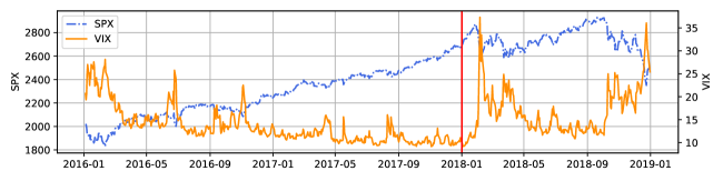
Figure 1: Series of the SPX and the VIX for 2016–2018. The vertical red line indicates the dividing date, the left and the right of which correspond to the training period (2016–2017) and the test period (2018), respectively.

	SPX					VIX
	mean	deviation	skewness	kurtosis		mean	deviation	skewness	kurtosis
training	0.001	0.007	-0.530	4.379		-0.001	0.073	0.816	6.230
test	0.000	0.011	-0.435	3.319		0.004	0.100	2.170	13.289
all	0.000	0.008	-0.581	5.295		0.000	0.083	1.669	12.385

Table 1: Moments for the log-return series of the SPX and the VIX for the data period.

We obtain options data on the SPX and the VIX from 2016 to 2018 from the CBOE data shop. We filter them out if their daily trades are below 50, if their prices do not reach 0.5 point, or if they expire within 3 days. We then split the data into a training set for 2016–2017 (235,227 SPX options and 46,516 VIX options) and a test set for 2018 (176,866 SPX options and 23,347 VIX options). Figure 1 shows the series of the SPX and the VIX for the data period. The vertical red line indicates the dividing date, the left and the right of which correspond to the training period and the test period, respectively. Many financial crises arose during the period: Chinese stock market turbulence (early 2016), Brexit (late 2016), and US stock market downturn (2018). It is clear that the SPX falls sharply and the VIX increases dramatically during each crisis. Table 1 summarizes the moments for the log-returns of both series for the data period. The VIX returns move in a much more volatile way than the SPX returns move. In addition, the SPX returns show negative skewness and weak kurtosis ($>3$), while the VIX returns show positive skewness and strong kurtosis ($\gg 3$). These findings imply that VIX options tend to be more expensive and riskier than SPX options are.

We adopt a two-step approach for calibrations for the Heston model and our model. Specifically, we perform a step-by-step calibration, in which the prices for specific kinds of products (e.g., SPX option) among all price data are used for parameter estimation for each step only. Such an approach is often observed in various studies in the literature (Bayer et al., 2013; Goutte et al., 2017). We first attempt to find the parameters $\kappa$, $\theta$, $\sigma$, and $\epsilon$ to control VIX option prices, and the other parameters $\rho$, $W_{3}^{\epsilon}$ are sought with SPX option prices. Note that the VIX option prices may be more sensitive to the parameters $\kappa$, $\theta$, and $\sigma$ than the SPX option prices. Because a highly precise optimization needs highly sensitive Greeks, it seems reasonable to prefer VIX options to SPX options for an estimation of the parameters $\kappa$, $\theta$, and $\sigma$. We first define the method for the Heston model with the four parameters $\kappa,\theta,\sigma$, and $\rho$ as follows.

1. First, perform calibration with VIX options

   $$\underset{\kappa,\theta,\sigma}{{\rm argmin}}\sum_{i\in I}\left(\sum_{j\in J_{v,i}}\left(\frac{P_{v}^{mdl}\left(z_{i},\kappa,\theta,\sigma;t_{i,}K_{j},T_{j}\right)-P_{v}^{mkt}\left(t_{i,},K_{j},T_{j}\right)}{0.1+P_{v}^{mkt}\left(t_{i,},K_{j},T_{j}\right)}\right)^{2}\right)$$

   such that

   $${\rm VIX}_{i}^{mkt}=\sqrt{b_{2}^{*}z_{i}+b_{4}^{*}\theta}.$$ (8)

   where $b_{2}^{*}=a_{2}^{*}/2$ and $b_{4}^{*}=\left(1+a_{4}^{*}\right)/2$.

2. Second, perform calibration with SPX options

$$\underset{\rho}{{\rm argmin}}\sum_{i\in I}\left(\sum_{j\in J_{s,i}}\left(\frac{P_{s}^{mdl}\left(\rho;t_{i,}K_{j},T_{j};z_{i},\kappa,\theta,\sigma\right)-P_{s}^{mkt}\left(t_{i,},K_{j},T_{j}\right)}{0.1+P_{s}^{mkt}\left(t_{i,},K_{j},T_{j}\right)}\right)^{2}\right).$$

The superscripts $mkt$ and $mdl$ are used to indicate the market price and the model price for an option, respectively. $I$ is the index set of the dates for the training set. $J_{v,i}$ and $J_{s,i}$ are the index sets of the VIX options and the SPX options, respectively, on the $i$th date. We explain the two-step method for our model with the six parameters $\kappa,\theta,\sigma,\rho,\epsilon$, and $W_{3}^{\epsilon}$ as follows.

1. First, perform calibration with VIX options

   $$\underset{\kappa,\theta,\sigma,\epsilon}{{\rm argmin}}\sum_{i\in I}\left(\underset{y_{i},z_{i}}{{\rm argmin}}\sum_{j\in J_{v,i}}\left(\frac{P_{v}^{mdl}\left(y_{i},z_{i},\kappa,\theta,\sigma,\epsilon;t_{i,}K_{j},T_{j}\right)-P_{v}^{mkt}\left(t_{i,},K_{j},T_{j}\right)}{0.1+P_{v}^{mkt}\left(t_{i,},K_{j},T_{j}\right)}\right)^{2}\right)$$

   such that

   $${\rm VIX}_{i}^{mkt}=\sqrt{a_{1}^{\epsilon}y_{i}+a_{2}^{\epsilon}z_{i}+\left(a_{3}^{\epsilon}+a_{4}^{\epsilon}\right)\theta}.$$ (9)

2. Second, perform calibration with SPX options

$$\underset{\rho,W_{3}^{\epsilon}}{{\rm argmin}}\sum_{i\in I}\left(\sum_{j\in J_{s,i}}\left(\frac{P_{s}^{mdl}\left(\rho,W_{3}^{\epsilon};t_{i,}K_{j},T_{j};y_{i},z_{i},\kappa,\theta,\sigma\right)-P_{s}^{mkt}\left(t_{i,},K_{j},T_{j}\right)}{0.1+P_{s}^{mkt}\left(t_{i,},K_{j},T_{j}\right)}\right)^{2}\right).$$

Note that, under the Heston model, $z_{i}$ is uniquely determined by the relationship (8) between the model and the VIX. By contrast, under our model, $y_{i}$ and $z_{i}$ cannot be uniquely determined by the relationship (9), which is why we also minimize the daily objective with respect to $y_{i}$ and $z_{i}$ for each $i$th date. Because this process requires large computational resources, the calibrations for both models are implemented based upon C++ and OpenMP, and executed in parallel on 24 CPU cores of two Intel Xeon Gold 5118. As a result, we obtain the following parameters for each model: $\kappa=3.43$, $\theta=0.0400$, $\sigma=0.424$, and $\rho=-1$ for the Heston model and $\kappa=3.58$, $\theta=0.021$ $\sigma=0.347$, $\rho=-1$, $\epsilon=0.0096$, and $W_{3}^{\epsilon}=0.0150$ for our model. Note that the two time scales for our model are well separated, as $\kappa=3.58$ and $1/\epsilon=104.17$.

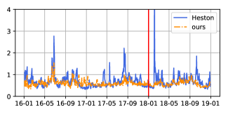
(a) errors for SPX options

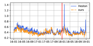
(b) errors for VIX options

Figure 2: Comparison of daily errors of both models by product types for 2016–2018. The vertical red line indicates the dividing date, the left and the right of which are the training period (2016–2017) and the test period (2018), respectively.

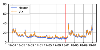
(a) $\sqrt{z_{i}}$ for the Heston model

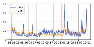
(b) $\sqrt{y_{i}+z_{i}}$ for our model

Figure 3: Spot volatilities of both models for 2016–2018. The vertical red line indicates the dividing date.

Figure 2 compares the daily errors of the Heston model and our model for the data period. The left and right figures indicate the errors for the SPX options and the VIX options, respectively. As before, the vertical red line represents the dividing date for the training data and the test data, respectively. At first glance, our model produces less errors, and it is more robust than the Heston model. Precisely, our model reduces the errors on the training sets of the SPX and the VIX options by 9.9% and 13.2%, respectively, and decreases the errors on the test sets of the SPX and the VIX options by 13.0% and 16.5%, respectively, compared with the Heston model (refer to C). In particular, the Heston model gives fairly large errors for particular dates. We can postulate a plausible reason for those phenomena from Figure 3, which draws the spot volatilities of both models for the data period. In the figure, the hidden process for our model appears to be more dynamic than that for the Heston model. This is because the spot volatility $\sqrt{z_{i}}$ for the Heston model is strongly correlated with the VIX but $\sqrt{y_{i}+z_{i}}$ for our model is not. Our model captures short-term volatility that is difficult to detect and produces a more volatile process. If our model is assumed to be correct, we conclude that the spot volatilities for the Heston model are fairly often biased, especially when sudden strong shocks impact the market. The bias eventually results in large fitting or prediction errors of the Heston model for short-term products, as shown in Table C. The table sums up the errors separately by time to maturity. The table results confirm that our model performs better than the Heston model as the time to maturity for an option becomes shorter, provided that the time to expiration is not too short. Note that the asymptotic method is valid when the time to maturity is not too short.

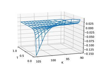
(a) $y=0.0234$, $z=0.0194$

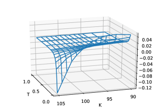
(b) $y=0.0110$, $z=0.0203$

Figure 4: Two differences between the SPX implied volatility surfaces from the corrected and uncorrected prices. Here, $z=0.0197$ for the uncorrected case.

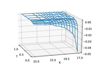
(a) $y=0.0234$, $z=0.0194$

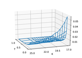
(b) $y=0.0110$, $z=0.0203$

Figure 5: Two differences between the VIX implied volatility surfaces from the corrected and uncorrected prices.

Furthermore, implied volatility surfaces for SPX options and VIX options clearly show how appropriate our model is for fitting to short-term products. To define the implied volatility for VIX options consistently , we first consider the following simple model:

$$d{\rm VIX}_{t}=\sigma dW_{t}.$$

In other words, ${\rm VIX}_{T}$ follows the normal distribution $N\left({\rm VIX}_{t},\sigma\sqrt{T-t}\right)$ under the model. Then, it is easy to show that the price $c$ of a VIX call option with maturity $T$ and strike $K$ is given by

$$c\left({\rm VIX}_{t}\right)=\left({\rm VIX}_{t}-K\right)N\left(\frac{{\rm VIX}_{t}-K}{\sigma\sqrt{T-t}}\right)+\sigma\sqrt{T-t}\ n\left(\frac{{\rm VIX}_{t}-K}{\sigma\sqrt{T-t}}\right)$$

where $N$ and $n$ are the cumulative distribution function and the probability density function of the unit Gaussian distribution, respectively. As a result, for the market price $c^{mkt}$, the corresponding implied volatility for the VIX option can be defined as $\sigma^{imp}$ to match the model price with $c^{mkt}$.

We now generate implied volatility surfaces $\sigma_{0,1}^{imp}$ from the corrected prices $P_{s,0}\left(z\right)+P_{s,1}\left(z\right)$ and $P_{v,0}\left(z\right)+P_{v,1}\left(y,z\right)$ with the estimated parameters $\kappa=3.58$, $\theta=0.021$ $\sigma=0.347$, $\rho=-1$, $\epsilon=0.0096$, and $W_{3}^{\epsilon}=0.0150$ for two hidden states $\left(y,z\right)=\left(0.0234,0.0194\right)$ and $\left(y,z\right)=\left(0.0110,0.0203\right)$. We also generate an additional implied volatility surface $\sigma_{0}^{imp}$ from the uncorrected prices $P_{s,0}\left(z\right)$ and $P_{v,0}\left(z\right)$ for hidden state $z=0.0197$, which is equivalent to generating the surface using the corrected prices with the same parameters as the preceding case but $\epsilon=0$ and $W_{3}^{\epsilon}=0$. All the hidden states $y$, $z$ are chosen so that the model value of the VIX is $20$, that is, ${\rm VIX}_{t}=20$ in the relationship (6).

Figures 4 and 5 present the differences $\sigma_{0,1}^{imp}-\sigma_{0}^{imp}$ for the SPX cases and the VIX cases, respectively. The figures confirm once again that the corrected terms $P_{s,1}$ and $P_{v,1}$ allow excellent short-term flexibility, and thereby capture the fluctuations in the slope and the level of the volatility smirk. Based on Figure 4, $P_{s,1}$ may make short-term in-the-money (SITM) options more expensive than short-term out-of-the-money (SOTM) options in a somewhat robust way. However, based on Figure 5, a subtle change of $z$ in our model seems to lead to a significantly different short-term VIX market. When the short-term state $y$ is smaller than the mid-term state $z$, as in the right figure, $P_{v,1}$ makes the SITM options more expensive than the SOTM options, as in the SPX cases, while $P_{v,1}$ works in the opposite way when $y$ is larger than $z$, as in the left figure. These phenomena for VIX volatility surfaces may occur because $Y_{t}$ quickly converges $Z_{t}$ in our model. If $y>z$, the spot volatility might decline in the short term, which means that the VIX SITM calls would probably not be exercised. If $y<z$, the spot volatility might increase for a short while, which would increase the value of the VIX SOTM call. This is simply the mechanism of our model showing diverse expression for the short-term VIX market in spite of the constraint (6).

5 Concluding remarks

In this paper, we study consistent and efficient pricing of SPX and VIX options under a new two-factor stochastic volatility model. Specifically, this two-factor model is proposed by adding a fast mean-reverting factor into the Heston model. Doing so facilitates joint pricing of the SPX option and the VIX option. In practice, joint modeling of both options is important, because an arbitrage relationship exists between the SPX option market and the VIX option market. Moreover, joint modeling leads to a calibration based on extensive market data, including SPX data and VIX data. Since our analytic solutions are derived as one-dimensional integrals, it is obvious that the pricing solutions are computationally very efficient. Our experiment using hundreds of thousands of options shows that the model reduces the errors by 9.9-16.5%, compared to the single-scale model of Heston. The error reduction is possible because the additional factor reflects short-term impacts on the market, which is difficult to achieve with only one factor.

In fact, non-affine models have been less studied for explicit pricing formulas because the involved problems are hard to solve. But the models are more suitable to express actual dynamics (see Mencia and Sentana (2013) and Kaeck and Alexander (2013)). In this context, our models should be extended to have a non-affine form. We leave the topic as future work.

Declarations of interest : none.

References

Appendix A Derivation of analytic formula for SPX options

Putting $P_{s}^{\epsilon}=P_{s,0}+\sqrt{\epsilon}P_{s,1}+\epsilon P_{s,2}+\epsilon\sqrt{\epsilon}P_{s,3}+\cdots$ into the PDE (3),

$$\frac{1}{\epsilon}\mathcal{L}_{s,0}P_{s,0}+\frac{1}{\sqrt{\epsilon}}\left(\mathcal{L}_{s,0}P_{s,1}+\mathcal{L}_{s,1}P_{s,0}\right)+\left(\mathcal{L}_{s,0}P_{s,2}+\mathcal{L}_{s,1}P_{s,1}+\mathcal{L}_{s,2}P_{s,0}\right)$$

$$\qquad\qquad\qquad\qquad\qquad\qquad+\sqrt{\epsilon}\left(\mathcal{L}_{s,0}P_{s,3}+\mathcal{L}_{s,1}P_{s,2}+\mathcal{L}_{s,2}P_{s,1}\right)+\cdots=0.$$

As mentioned in Theorem 1, we intend for the sum of the leading term $P_{s,0}$ and the first non-zero correction term $P_{s,1}$ to approximate $P_{s}^{\epsilon}$ within accuracy $O\left(\epsilon\right)$, that is, $\left|P_{s}^{\epsilon}-\left(P_{s,0}+\sqrt{\epsilon}P_{s,1}\right)\right|<C\epsilon$ for some positive $C$. For this purpose, the following equations should be satisfied:

$$\mathcal{L}_{s,0}P_{s,0}=0,$$ (10)

$$\mathcal{L}_{s,0}P_{s,1}+\mathcal{L}_{s,1}P_{s,0}=0,$$ (11)

$$\mathcal{L}_{s,0}P_{s,2}+\mathcal{L}_{s,1}P_{s,1}+\mathcal{L}_{s,2}P_{s,0}=0,$$ (12)

$$\mathcal{L}_{s,0}P_{s,3}+\mathcal{L}_{s,1}P_{s,2}+\mathcal{L}_{s,2}P_{s,1}=0.$$ (13)

$P_{s,0}$ should not depend on $y$ so that the Poisson equation (10) has a solution. This means that $P_{s,1}$ also does not depend on $y$ owing to (11). From (12), we then obtain

$$\mathcal{L}_{s,0}P_{s,2}+\mathcal{L}_{s,2}P_{s,0}=0.$$ (14)

Thus, the centering condition for $\mathcal{L}_{s,0}$ for the Poisson equation (14) results in the following PDE (4) for $P_{s,0}$:

$$\left\langle\mathcal{L}_{s,2}P_{s,0}\right\rangle=\left\langle\mathcal{L}_{s,2}\right\rangle P_{s,0}=0,$$ (15)

$$P_{s,0}\left(T,x,z\right)=\left(x-K\right)^{+},$$

where $\left\langle\cdot\right\rangle$ is the expectation with respect to the invariant distribution $\Phi$ for $Y_{t}$, that is, $\left\langle f\right\rangle=\int f\left(y\right)\Phi\left(y\right)dy$. Moreover, because $Y_{t}$ is a CIR process, $Y_{\infty}\sim\Gamma\left(\gamma,\nu^{2}\right)$, which means that the density function for $Y_{\infty}$ is

$$\Phi\left(w\right)=\frac{1}{\nu^{2\gamma}\Gamma\left(\gamma\right)}w^{\gamma-1}e^{-\left(w/\nu^{2}\right)}\boldsymbol{1}_{\left(0,\infty\right)}\left(w\right),$$

where $\gamma=\frac{z}{\nu^{2}}$. The centering condition indicates that $\left\langle g\right\rangle=0$ should hold for Poisson equation $\mathcal{L}f+g=0$. The condition is necessary for a Poisson equation to have a solution.

In addition, (14) yields the following equation:

$$P_{s,2} =-\mathcal{L}_{s,0}^{-1}\left(\mathcal{L}_{s,2}-\left\langle\mathcal{L}_{s,2}\right\rangle\right)P_{s,0}+c\left(t,x,z\right)$$

$$=-\frac{1}{2}x^{2}\phi\left(y,z\right)\partial_{xx}^{2}P_{s,0}+c\left(t,x,z\right),$$ (16)

where

$$\mathcal{L}_{s,0}\phi\left(y,z\right)=y-z.$$ (17)

In fact, we show $\phi\left(y,z\right)=z-y$, the proof of which is given in B. On one hand, if we put (16) into (13) and use the centering condition for $\mathcal{L}_{s,0}$ in (13), we achieve the PDE (5) for $P_{s,1}$ in the following ways:

$$\left\langle\mathcal{L}_{s,2}\right\rangle P_{s,1} =-\left\langle\mathcal{L}_{s,1}P_{s,2}\right\rangle$$

$$=\frac{1}{\sqrt{2}}\eta\nu\left\langle y\phi_{y}\left(y,z\right)\right\rangle x\partial_{x}\left(x^{2}\partial_{xx}^{2}P_{0}\right)$$

$$=W_{3}zx\partial_{x}\left(x^{2}\partial_{xx}^{2}\right)P_{s,0}.$$ (18)

with the corresponding final condition

$$P_{s,1}\left(T,x,z\right)=0,$$

where $W_{3}=-\frac{1}{\sqrt{2}}\eta\nu$ (recall that $W_{3}^{\epsilon}=-\frac{1}{\sqrt{2}}\eta\nu\sqrt{\epsilon}$, i.e., $W_{3}=W_{3}^{\epsilon}/\sqrt{\epsilon}$).

On the other hand, if $\xi:=2z$, equations (15) and (18) are transformed as follows, and they are associated with the PDE operator $\mathcal{L}_{H}$ for the Heston model, whose parameters are the mean reversion rate of $\kappa$, the long-run variance $2\theta$, the volatility of variance $\sqrt{2}\sigma$, and the correlation $\sqrt{2}\rho$ between stock price and its variance.

$$\mathcal{L}_{H}\tilde{P}_{s,0}\left(t,x,\xi\right)=0,$$

$$\mathcal{L}_{H}\tilde{P}_{s,1}\left(t,x,\xi\right)=\frac{1}{2}W_{3}\xi x\partial_{x}\left(x^{2}\partial_{xx}^{2}\right)\tilde{P}_{s,0}\left(t,x,\xi\right),$$ (19)

where

$$\mathcal{L}_{H}=\partial_{t}+rx\partial_{x}+\kappa\left(2\theta-\xi\right)\partial_{\xi}+\frac{1}{2}x^{2}\xi\partial_{xx}^{2}+\frac{1}{2}\left(\sqrt{2}\sigma\right)^{2}\xi\partial_{\xi\xi}^{2}+\left(\frac{1}{\sqrt{2}}\rho\right)\left(\sqrt{2}\sigma\right)x\xi\partial_{x\xi}^{2}-r.$$

Similar to Fouque and Lorig (2011), by utilizing the feasibility of the Heston model, we can achieve the following solutions of the abovementioned PDEs:

$$\tilde{P}_{s,0}\left(t,x,\xi\right)=\frac{e^{-r\tau}}{2\pi}\int_{\mathbb{}}e^{-ikq}\hat{G}\left(\tau,k,2\xi\right)\hat{h}\left(k\right)dk,$$

$$\tilde{P}_{s,1}\left(t,x,\xi\right)=\frac{e^{-r\tau}}{2\pi}\int_{\mathbb{}}e^{-ikq}b\left(k\right)\left(\kappa\theta\hat{f}_{0}\left(\tau,k\right)+2z\hat{f}_{1}\left(\tau,k\right)\right)\hat{G}\left(\tau,k,\xi\right)\hat{h}\left(k\right)dk,$$

where $\tau=T-t$, $q=r\tau+\log x$,

$$b\left(k\right) =-\frac{1}{2}W_{3}\left(ik^{3}+k^{2}\right),$$

$$\hat{f}_{0}\left(\tau,k\right) =\int_{0}^{\tau}\hat{f}_{1}\left(t,k\right)dt,$$

$$\hat{f}_{1}\left(\tau,k\right) =\int_{0}^{\tau}\left(\frac{g\left(k\right)e^{sd\left(k\right)}-1}{g\left(k\right)e^{\tau d\left(k\right)}-1}\right)^{2}e^{d\left(k\right)\left(\tau-s\right)}ds,$$

and $\hat{G}\left(\tau,k,z\right)$, $\hat{h}\left(k\right)$, $d\left(k\right)$, and $g\left(k\right)$ are defined in Theorem 1. To compute $\tilde{P}_{s,0}$ and $\tilde{P}_{s,1}$, numerical integrations need to be associated with a single integration and a triple integration. However, as in the foregoing discussion in 3.1, numerical methods for the triple integration are too computationally intensive. Fortunately, we can further simplify $\hat{f}_{0}$ and $\hat{f}_{1}$, because the right-hand side of (19) is linear with respect to $\xi$. The induction process is given in detail as follows:

$$\hat{f}_{1}\left(\tau,k\right) =\int_{0}^{\tau}\frac{\left(g\left(k\right)e^{sd\left(k\right)}-1\right)^{2}}{\left(g\left(k\right)e^{\tau d\left(k\right)}-1\right)^{2}}e^{d\left(k\right)\left(\tau-s\right)}ds$$

$$=\frac{e^{\tau d\left(k\right)}}{\left(g\left(k\right)e^{\tau d\left(k\right)}-1\right)^{2}}\int_{0}^{\tau}\frac{\left(g\left(k\right)e^{sd\left(k\right)}-1\right)^{2}}{e^{sd\left(k\right)}}ds$$

$$=\left(\frac{e^{\tau d\left(k\right)}}{\left(g\left(k\right)e^{\tau d\left(k\right)}-1\right)^{2}}\right)\left(\frac{1}{d\left(k\right)}\left(g\left(k\right)^{2}e^{\tau d\left(k\right)}-2\tau d\left(k\right)g\left(k\right)-e^{-\tau d\left(k\right)}+1-g\left(k\right)^{2}\right)\right)+1$$

$$=\frac{e^{\tau d\left(k\right)}\left(g\left(k\right)^{2}\left(e^{\tau d\left(k\right)}-1\right)-2\tau d\left(k\right)g\left(k\right)+1\right)-1}{d\left(k\right)\left(g\left(k\right)e^{\tau d\left(k\right)}-1\right)^{2}}.$$

If $I\left(\tau,k\right):=\frac{e^{\tau d\left(k\right)}}{\left(g\left(k\right)e^{\tau d\left(k\right)}-1\right)^{2}}$, $\hat{f}_{1}\left(\tau,k\right)=I\left(t,k\right)\int_{0}^{t}\frac{1}{I\left(s,k\right)}ds$ from the second line of the above equations. Thus, we can obtain

$$\hat{f}_{0}\left(\tau,k\right) =\int_{0}^{\tau}I\left(t,k\right)\int_{0}^{t}\frac{1}{I\left(s,k\right)}dsdt$$

$$=\int_{0}^{\tau}\frac{1}{I\left(s,k\right)}\int_{s}^{\tau}I\left(t,k\right)dtds$$

$$=\int_{0}^{\tau}\frac{\left(g\left(k\right)e^{sd\left(k\right)}-1\right)^{2}}{e^{sd\left(k\right)}}\left(\frac{1}{d\left(k\right)g\left(k\right)-d\left(k\right)g\left(k\right)^{2}e^{\tau d\left(k\right)}}-\frac{1}{d\left(k\right)g\left(k\right)-d\left(k\right)g\left(k\right)^{2}e^{sd\left(k\right)}}\right)ds$$

$$=\frac{2\tau d\left(k\right)g\left(k\right)+g^{2}\left(k\right)-1}{d^{2}\left(k\right)g\left(k\right)\left(g\left(k\right)e^{\tau d\left(k\right)}-1\right)}+\frac{\tau d\left(k\right)g\left(k\right)-g\left(k\right)-1}{d^{2}\left(k\right)g\left(k\right)}.$$

Appendix B Solution for Poisson equation (17)

By the spectral theory, solution $\phi$ for Poisson equation (17) can be found as follows:

$$\phi\left(y,z\right)=z-y.$$

Now, we briefly explain the way to find $\phi$. It is known that the operator $\mathcal{L}_{s,0}$ has the eigenvalues $\lambda_{n}=-n$ $\left(n\in\mathbb{N}\right)$ and the family of eigenfunctions $\psi_{n}$ associated with eigenvalue $\lambda_{n}$ (i.e., $\mathcal{L}_{s,0}\psi_{n}=\lambda_{n}\psi_{n}$) is

$$\psi_{n}\left(y\right) =\sqrt{\frac{n!\Gamma\left(\gamma\right)}{\Gamma\left(n+\gamma\right)}}L_{n}\left(\frac{y}{\nu^{2}}\right),$$

where $\gamma=\frac{z}{\nu^{2}}$ and $L_{n}$ is an $n$-order Legendre polynomial, that is, $L_{n}\left(w\right)=\frac{w^{1-\gamma}e^{w}}{n!}\frac{d^{n}}{dw^{n}}\left(w^{n+\gamma-1}e^{-w}\right)$. It is also known that $\psi_{n}$ form a complete orthogonal basis of the Hilbert space $L^{2}\left(\Phi\right)$. $\Phi$ is the invariant distribution of $Y_{t}$, which is defined in the foregoing section. Thus, $y-z\in L^{2}\left(\Phi\right)$ can be expressed as

$$y-z=\sum_{n\geq 0}c_{n}\psi_{n}\left(y\right),$$ (20)

where $c_{n}=\left\langle\left(y-z\right)\psi_{n}\right\rangle$. For any $n$, $c_{n}$ are explicitly calculated as follows:

$$c_{n}=\begin{cases}-\nu\sqrt{z}&{\rm if}\;n=1\\ 0&{\rm otherwise}\end{cases}$$ (21)

We provide the induction process for the above formula (21). First, $c_{0}$ can be easily obtained as follows:

$$c_{0}=\left\langle\left(y-z\right)\psi_{0}\right\rangle=\left\langle y-z\right\rangle=0.$$

In addition, $c_{1}$ is computed as follows:

$$c_{1} =\left\langle\left(y-z\right)\psi_{1}\right\rangle$$

$$=\sqrt{\frac{\Gamma\left(\gamma\right)}{\Gamma\left(1+\gamma\right)}}\int_{0}^{\infty}\left(y-z\right)\left(\gamma-\frac{y}{\nu^{2}}\right)\Phi\left(y\right)dy$$

$$=\sqrt{\frac{1}{\gamma}}\int_{0}^{\infty}\left(-\frac{1}{\nu^{2}}y^{2}+\left(\frac{z}{\nu^{2}}+\gamma\right)y-\gamma z\right)\Phi\left(y\right)dy$$

$$=-\nu\sqrt{z}.$$

It is also proved that $c_{n}$ for $n\geq 2$ are zero, because we can show the following equation:

$$\int_{0}^{\infty}y\left[\left(\frac{y}{\nu^{2}}\right)^{1-\gamma}e^{\frac{y}{\nu^{2}}}\frac{d^{n}}{dy^{n}}\left(\left(\frac{y}{\nu^{2}}\right)^{n+\gamma-1}e^{-\frac{y}{\nu^{2}}}\right)\right]\left[y^{\gamma-1}e^{-\left(y/\nu^{2}\right)}\right]dy$$

$$=\nu^{2\gamma-2}\int_{0}^{\infty}y\frac{d^{n}}{dy^{n}}\left(\left(\frac{y}{\nu^{2}}\right)^{n+\gamma-1}e^{-\frac{y}{\nu^{2}}}\right)dy$$

$$=-\nu^{2\gamma-2}\int_{0}^{\infty}\frac{d^{n-1}}{dy^{n-1}}\left(\left(\frac{y}{\nu^{2}}\right)^{n+\gamma-1}e^{-\frac{y}{\nu^{2}}}\right)dy$$

$$=-\nu^{2\gamma-2}\left[\frac{d^{n-2}}{dy^{n-2}}\left(\left(\frac{y}{\nu^{2}}\right)^{n+\gamma-1}e^{-\frac{y}{\nu^{2}}}\right)\right]_{0}^{\infty}$$

$$=\nu^{2\gamma-2}\left[\left(n+\gamma-1\right){\rm th\ degree\ polynomial\ without\ constant\ term}\times e^{-\frac{y}{\nu^{2}}}\right]_{0}^{\infty}$$

$$=0.$$

Therefore, we eventually obtain the following $\phi$ by (20) and (21):

$$\phi\left(y,z\right) =\frac{c_{1}\psi_{1}\left(y\right)}{\lambda_{1}}$$

$$=\frac{z}{\gamma}\left(\gamma-\frac{y}{\nu^{2}}\right)$$

$$=z-y.$$

Appendix C Errors in the empirical test

[In-sample errors for 2016–2017 options data] $\tau<0.05$ $0.05\leq\tau<0.1$ $0.1\leq\tau<0.2$ $\tau\geq 0.2$ total Heston ours o/h Heston ours o/h Heston ours o/h Heston ours o/h Heston ours o/h SPX mean 0.454 0.478 105% 0.509 0.419 82.2% 0.522 0.466 89.3% 0.494 0.557 113% 0.489 0.441 90.1% std 0.490 0.424 0.636 0.443 0.652 0.552 0.551 0.714 0.587 0.437 Heston ours o/h Heston ours o/h Heston ours o/h Heston ours o/h Heston ours o/h VIX mean 0.278 0.266 95.6% 0.402 0.344 85.5% 0.423 0.372 88.1% 0.437 0.391 89.5% 0.380 0.330 86.8% std 0.242 0.249 0.260 0.250 0.257 0.249 0.254 0.249 0.261 0.251
[Out-of-sample errors for 2018 options data] $\tau<0.05$ $0.05\leq\tau<0.1$ $0.1\leq\tau<0.2$ $\tau\geq 0.2$ total Heston ours o/h Heston ours o/h Heston ours o/h Heston ours o/h Heston ours o/h SPX mean 0.500 0.472 94.5% 0.535 0.441 82.4% 0.526 0.452 85.8% 0.485 0.470 97.0% 0.521 0.453 87.0% std 0.538 0.373 0.813 0.369 0.871 0.412 0.720 0.475 0.717 0.371 Heston ours o/h Heston ours o/h Heston ours o/h Heston ours o/h Heston ours o/h VIX mean 0.321 0.259 80.6% 0.380 0.320 84.1% 0.393 0.338 86.1% 0.402 0.358 89.0% 0.369 0.308 83.5% std 0.294 0.247 0.301 0.232 0.282 0.235 0.267 0.240 0.300 0.236

Errors in empirical test based on 2016–2018 options data. The results are shown separately by time to maturity. The abbreviation “o/h” means the value obtained by dividing the error for our model by the corresponding error for the Heston model.

References

• Bayer et al. (2013) Bayer, C., Gatheral, J., Karlsmark, M., 2013. Fast ninomiya–victoir calibration of the double-mean-reverting model. Quantitative Finance 13 (11), 1813–1829.
• Brigo and Mercurio (2007) Brigo, D., Mercurio, F., 2007. Interest rate models-theory and practice: with smile, inflation and credit. Springer Science & Business Media.
• Carr and Madan (1998) Carr, P., Madan, D., 1998. Towards a theory of volatility trading. Volatility: New estimation techniques for pricing derivatives 29, 417–427.
• Cheng et al. (2012) Cheng, J., Ibraimi, M., Leippold, M., Zhang, J. E., 2012. A remark on lin and chang’s paper ‘consistent modeling of s&p 500 and vix derivatives’. Journal of Economic Dynamics and Control 36 (5), 708–715.
• Chernov et al. (2003) Chernov, M., Gallant, A. R., Ghysels, E., Tauchen, G., 2003. Alternative models for stock price dynamics. Journal of Econometrics 116 (1-2), 225–257.
• Christoffersen et al. (2009) Christoffersen, P., Heston, S., Jacobs, K., 2009. The shape and term structure of the index option smirk: Why multifactor stochastic volatility models work so well. Management Science 55 (12), 1914–1932.
• Cont and Kokholm (2013) Cont, R., Kokholm, T., 2013. A consistent pricing model for index options and volatility derivatives. Mathematical Finance: An International Journal of Mathematics, Statistics and Financial Economics 23 (2), 248–274.
• Duffie et al. (2000) Duffie, D., Pan, J., Singleton, K., 2000. Transform analysis and asset pricing for affine jump-diffusions. Econometrica 68 (6), 1343–1376.
• Fouque and Lorig (2011) Fouque, J.-P., Lorig, M. J., 2011. A fast mean-reverting correction to heston’s stochastic volatility model. SIAM Journal on Financial Mathematics 2 (1), 221–254.
• Fouque et al. (2011) Fouque, J.-P., Papanicolaou, G., Sircar, R., Sølna, K., 2011. Multiscale stochastic volatility for equity, interest rate, and credit derivatives. Cambridge University Press.
• Fouque and Saporito (2018) Fouque, J.-P., Saporito, Y. F., 2018. Heston stochastic vol-of-vol model for joint calibration of vix and s&p 500 options. Quantitative Finance 18 (6), 1003–1016.
• Gallant et al. (1999) Gallant, A. R., Hsu, C.-T., Tauchen, G., 1999. Using daily range data to calibrate volatility diffusions and extract the forward integrated variance. Review of Economics and Statistics 81 (4), 617–631.
• Gatheral (2008) Gatheral, J., 2008. Consistent modeling of spx and vix options. In: Bachelier Congress. p. 3.
• Goutte et al. (2017) Goutte, S., Ismail, A., Pham, H., 2017. Regime-switching stochastic volatility model: estimation and calibration to vix options. Applied Mathematical Finance 24 (1), 38–75.
• Huh et al. (2018) Huh, J., Jeon, J., Kim, J.-H., 2018. A scaled version of the double-mean-reverting model for vix derivatives. Mathematics and Financial Economics 12 (4), 495–515.
• Kaeck and Alexander (2012) Kaeck, A., Alexander, C., 2012. Volatility dynamics for the s&p 500: Further evidence from non-affine, multi-factor jump diffusions. Journal of Banking & Finance 36 (11), 3110–3121.
• Kaeck and Alexander (2013) Kaeck, A., Alexander, C., 2013. Continuous-time vix dynamics: On the role of stochastic volatility of volatility. International Review of Financial Analysis 28, 46–56.
• Lian and Zhu (2013) Lian, G.-H., Zhu, S.-P., 2013. Pricing vix options with stochastic volatility and random jumps. Decisions in Economics and Finance 36 (1), 71–88.
• Lin and Chang (2009) Lin, Y.-N., Chang, C.-H., 2009. Vix option pricing. Journal of Futures Markets: Futures, Options, and Other Derivative Products 29 (6), 523–543.
• Lin and Chang (2010) Lin, Y.-N., Chang, C.-H., 2010. Consistent modeling of s&p 500 and vix derivatives. Journal of Economic Dynamics and Control 34 (11), 2302–2319.
• Mencia and Sentana (2013) Mencia, J., Sentana, E., 2013. Valuation of vix derivatives. Journal of Financial Economics 108 (2), 367–391.