Design of Globally Exponentially Convergent Continuous Observers for Velocity Bias and State for Systems on Real Matrix Groups

Abstract

We propose globally exponentially convergent continuous observers for invariant kinematic systems on finite-dimensional matrix Lie groups. Such an observer estimates, from measurements of landmarks, vectors and biased velocity, both the system state and the unknown constant bias in velocity measurement, where the state belongs to the state-space Lie group and the velocity to the Lie algebra of the Lie group. The main technique is to embed a given system defined on a matrix Lie group into Euclidean space and build observers in the Euclidean space. The theory is illustrated with the special Euclidean group in three dimensions.

I Introduction

Consider an invariant kinematic system on a matrix Lie group $G$:

$$\dot{g}=g\xi$$

with $(g,\xi)\in G\times\mathfrak{g}$, where $G$ is embedded in $\mathbb{R}^{n\times n}$ and $\mathfrak{g}$ denotes the Lie algebra of $G$. Suppose that the velocity $\xi$ is measured with an additive unknown constant bias as

$$\xi_{\rm m}=\xi+b$$

where $b\in\mathfrak{g}$ is the constant unknown bias. Suppose also that we measure landmarks and vectors such that an $n\times n$ matrix-valued signal $A$ of the form

$$A=Fg$$

or

$$A=g^{-1}F$$

is available, where $F$ is an $n\times n$ invertible matrix. In this paper, we design continuous observers that globally and exponentially estimate $(g,b)$ with $\xi_{\rm m}$ and $A$, where it is assumed that the value of $F$ is available.

Relevant works are listed in the following. In [9], the authors proposed continuous observers that estimate $(g,b)$ with $\xi_{m}$ and homogeneous outputs. Their observers are uniformly locally exponentially stable, but not globally exponentially stable. A similar work was done in [8], where a gradient-like innovation term was used in the observer design. The observers therein are not globally exponentially stable but only uniformly locally exponentially stable. Gradient-like observers were also proposed in [10], but these observers are not globally exponentially convergent either.

To the best of our knowledge, our observers in the present paper are the first globally exponentially convergent continuous observers for velocity bias and state for kinematic systems on matrix Lie groups. One noticeable difference between the observers in [10, 8, 9] and ours is that our observers are designed in $\mathbb{R}^{n\times n}\times\mathfrak{g}$ instead of $G\times\mathfrak{g}$, where $G\subset\mathbb{R}^{n\times n}$, such that the Euclidean structure of $\mathbb{R}^{n\times n}$ is fully utilized without being constrained to the group structure of $G$. This type of observers built in Euclidean space is called geometry-free and they have been widely used for $\operatorname{SO}(3)$, e.g. [1, 11].

The paper is organized as follows. In Section II we propose various forms of globally exponentially convergent continuous observers for velocity bias and state for kinematic systems on matrix Lie groups. In Section III, we illustrate one of the observers proposed in Section II by applying it to the special Euclidean group $\operatorname{SE}(3)$. The paper is concluded in Section IV.

II Main Results

Let $G$ be a matrix Lie group that is a subgroup of ${\operatorname{GL}(n)}=\{A\in\mathbb{R}^{n\times n}\mid\det A\neq 0\}$, and let ${\mathfrak{g}}$ denote the Lie algebra of $G$. Since $G$ is a subgroup fo ${\operatorname{GL}(n)}$, we may assume that ${\mathfrak{g}}$ is a subalgebra of $(\mathbb{R}^{n\times n},[\,,])$, where $[\,,]$ is the usual matrix commutator defined by $[A,B]=AB-BA$ for all $A,B\in\mathbb{R}^{n\times n}$. Let $\operatorname{\pi_{{\mathfrak{g}}}}:\mathbb{R}^{n\times n}\rightarrow{\mathfrak{g}}$ denote the orthogonal projection onto ${\mathfrak{g}}$ with respect to the Euclidean inner product $\langle\,,\rangle$ that is defined by $\langle A,B\rangle=\operatorname{tr}(A^{T}B)$ for $A,B\in\mathbb{R}^{n\times n}$. Let $\|\|$ denote the Euclidean or Frobenius norm which is defined by $\|A\|=\sqrt{\langle A,A\rangle}$ for all $A\in\mathbb{R}^{n\times n}$. For a square matrix $A$, $\lambda_{\rm minx}(A)$ and $\lambda_{\rm max}(A)$ denote the minimum eigenvalue and the maximum eigenvalue of $A$, respectively. For any matrix $A$, $\sigma_{\rm min}(A)$ and $\sigma_{\rm max}(A)$ denote the minimum singular value and the maximum singular value of $A$, respectively. For any $A\in\mathbb{R}^{n\times n}$, $\|A\|^{2}=\sum_{i=1}^{n}\sigma_{i}^{2}(A)$, where $\sigma_{i}(A)$’s are the singular values of $A$. We have $\lambda_{\rm min}(A^{T}A)\|B\|^{2}\leq\langle AB,AB\rangle\leq\lambda_{\rm max}(A^{T}A)\|B\|^{2}$ for all $A\in\mathbb{R}^{n\times m}$ and $B\in\mathbb{R}^{m\times\ell}$, i.e. $\sigma^{2}_{\rm min}(A)\|B\|\leq\|AB\|\leq\sigma^{2}_{\rm max}(A)\|B\|$ for all $A\in\mathbb{R}^{n\times m}$ and $B\in\mathbb{R}^{m\times\ell}$. Refer to [2] for more about Lie groups in the context of geometric control and mechanics.

II-A Observer I

The invariant kinematic equation on a matrix Lie group $G\subset\mathbb{R}^{n\times n}$ is given by

$$\dot{g}=g\xi,$$ (1)

where $g\in G$ and $\xi\in{\mathfrak{g}}$. Suppose that there is given an arbitrary trajectory of the system $(g(t),\xi(t))\in G\times{\mathfrak{g}}$, $0\leq t<\infty$. We make the following three assumptions.

Assumption II.1.

A matrix-valued signal $A(t)\in\mathbb{R}^{n\times n}$ is available that can be expressed as

$$A={F}g,$$ (2)

where ${F}$ is a constant invertible matrix in $\mathbb{R}^{n\times n}$ and $g\in G$.

Assumption II.2.

A ${\mathfrak{g}}$-valued signal $\xi_{\rm m}(t)$ with bias is available and related to the true $\xi(t)\in{\mathfrak{g}}$ of as follows:

$$\xi_{\rm m}=\xi+b,$$

where $b\in{\mathfrak{g}}$ is an unknown constant bias vector.

Assumption II.3.

There are known constants $B_{\xi}>0$ and $B_{b}>0$ such that $\|\xi(t)\|\leq B_{\xi}$ for all $t\geq 0$ and $\|b\|\leq B_{b}$. There are numbers $L_{g}>0$ and $U_{g}>0$ such that

$$L_{g}\leq\sigma_{\rm min}(g(t))\leq\sigma_{\rm max}(g(t))\leq U_{g}$$

for all $t\geq 0$, where the knowledge on the values of $L_{g}$ and $U_{g}$ is not assumed.

We propose the following observer:

$$\dot{\bar{A}} =\bar{A}{\xi}_{\rm m}-A\bar{b}+k_{P}(A-\bar{A}),$$ (3a)

$$\dot{\bar{b}} =-k_{I}\operatorname{\pi_{{\mathfrak{g}}}}(A^{T}(A-\bar{A}))$$ (3b)

with $k_{P}>(B_{\xi}+B_{b})$ and $k_{I}>0$, where $(\bar{A},\bar{b})\in\mathbb{R}^{n\times n}\times{\mathfrak{g}}$ is an estimate of $(A,b)\in G\times{\mathfrak{g}}$. So, $({F}^{-1}\bar{A},\bar{b})\in\mathbb{R}^{n\times n}\times{\mathfrak{g}}$ becomes an estimate of $(g,b)\in G\times{\mathfrak{g}}$ by Assumption II.1. The global and exponentially convergent property of this observer is proven in the following theorem.

Theorem II.4.

Let

$$E_{A}=A-\bar{A},\quad e_{b}=b-\bar{b}.$$

Under Assumptions II.1 – II.3, for any $k_{P}>(B_{\xi}+B_{b})$ and $k_{I}>0$ there exist numbers $a>0$ and $C>0$ such that

$$\|E_{A}(t)\|+\|e_{b}(t)\|\leq C(\|E_{A}(0)\|+\|e_{b}(0)\|)e^{-at}$$ (4)

for all $t\geq 0$ and all $(\bar{A}(0),\bar{b}(0))\in\mathbb{R}^{n\times n}\times{\mathfrak{g}}$.

Proof.

See Appendix. ∎

Corollary II.5.

Suppose that Assumptions II.1 – II.3 hold, and let

$$E_{g}=g-{F}^{-1}\bar{A},\quad e_{b}=b-\bar{b}.$$

Then, there exist numbers $a>0$ and $C>0$ such that

$$\|E_{g}(t)\|+\|e_{b}(t)\|\leq C(\|E_{g}(0)\|+\|e_{b}(0)\|)e^{-at}$$ (5)

for all $t\geq 0$ and all $(\bar{A}(0),\bar{b}(0))\in\mathbb{R}^{n\times n}\times{\mathfrak{g}}$.

Proof.

Use $\|E_{g}\|/\|{F}^{-1}\|\leq\|E_{A}\|\leq\|{F}\|\|E_{g}\|$ and (4) with the constant $C$ redefined appropriately. ∎

Namely, the estimate $({F}^{-1}\bar{A}(t),\bar{b}(t))$ converges globally and exponentially to the true value $(g(t),b)$ as $t$ tends to $\infty$.

Remark II.6.

We can also build an observer that allows $\bar{b}$ to be in $\mathbb{R}^{n\times n}$ instead of $\mathfrak{g}$. The modified observer is given by

$$\dot{\bar{A}} =\bar{A}{\xi}_{\rm m}-A\bar{b}+k_{P}(A-\bar{A}),$$ (6a)

$$\dot{\bar{b}} =-k_{I}A^{T}(A-\bar{A}),$$ (6b)

where $(\bar{A},\bar{b})\in\mathbb{R}^{n\times n}\times\mathbb{R}^{n\times n}$. Notice that the projection operator $\operatorname{\pi_{{\mathfrak{g}}}}$ in (3b) is removed from (3b) to obtain (6b). Theorem II.4 and Corollary II.5 also hold for this observer, whose proof is almost identical to the proofs of Theorem II.4 and Corollary II.5, so it is left to the reader.

Remark II.7.

Assumption II.1 can be relaxed by allowing the matrix $F$ to be time-varying. More specifically, we make the following assumption: there are numbers $\ell_{\rm min}>0$ and $\ell_{\rm max}>0$ such that

$$\ell_{\rm min}\leq\sigma_{\rm min}({F}(t))\leq\sigma_{\rm max}({F}(t))\leq\ell_{\rm max}$$ (7)

for all $t\geq 0$. In this case, we propose the following observer:

$$\dot{\bar{A}} =\bar{A}{\xi}_{\rm m}-A{\bar{b}}+k_{P}(A-\bar{A})+\dot{F}{F}^{-1}A,$$

$$\dot{\bar{b}} =-k_{I}\operatorname{\pi_{{\mathfrak{g}}}}(A^{T}(A-\bar{A}))$$

with $k_{P}>0$ and $k_{I}>0$, where $(\bar{A},\bar{b})\in\mathbb{R}^{n\times n}\times{\mathfrak{g}}$ is an estimate of $(A,b)$. It is not difficult to show that Theorem II.4 and Corollary II.5 also hold for this observer with the relaxed assumption on ${F}(t)$ as above. Here, the knowledge on the values of $\ell_{\rm min}$ and $\ell_{\rm max}$ is not required here.

Remark II.8.

Since the estimate $F^{-1}\bar{A}$ may not lie in $G$ in general, one may need to project it to $G$ as an output of the observer although $F^{-1}\bar{A}(t)$ converges to $g(t)\in G$ as $t$ tends to infity. For example, if $G=\operatorname{SO}(3)$, then the usual polar decomposition can be used to define a projection from $\mathbb{R}^{3\times 3}$ to $\operatorname{SO}(3)$. Projection for $\operatorname{SE}(3)$ will be discussed in Section III. However, if one designs controllers in $\mathbb{R}^{n\times n}$ for an extension of (1) into $\mathbb{R}^{n\times n}$ as proposed in [4], then the direct use of $F^{-1}\bar{A}$ in feedback would be fine.

II-B Observer II

Recall the kinematic equation in (1). We now consider a case where the measurement matrix $A$ is related to the true signal $g(t)$ as $A=g^{-1}(t){F}$ instead of $A={F}g(t)$. Consequently, in place of Assumption II.9, let us make the following assumption:

Assumption II.9.

A matrix-valued signal $A(t)\in\mathbb{R}^{n\times n}$ is available that can be expressed as

$$A=g^{-1}{F},$$ (8)

where ${F}$ is a constant invertible matrix in $\mathbb{R}^{n\times n}$ and $g\in G$.

By (1), $A$ defined in (8) satisfies

$$\dot{A}=-\xi A.$$ (9)

Under Assumptions II.9, II.2 and II.3, we propose the following observer:

$$\dot{\bar{A}} =-{\xi}_{\rm m}\bar{A}+\bar{b}A+k_{P}(A-\bar{A}),$$ (10a)

$$\dot{\bar{b}} =k_{I}\operatorname{\pi_{{\mathfrak{g}}}}((A-\bar{A})A^{T})$$ (10b)

with $k_{P}>(B_{\xi}+B_{b})$ and $k_{I}>0$, where $(\bar{A},\bar{b})\in\mathbb{R}^{n\times n}\times{\mathfrak{g}}$ is an estimate of $(A,b)\in G\times{\mathfrak{g}}$.

Theorem II.10.

For the observer (10), let

$$E_{A}=A-\bar{A},\quad e_{b}=b-\bar{b}.$$

Under Assumptions II.9, II.2 and II.3, for any $k_{P}>(B_{\xi}+B_{b})$ and $k_{I}>0$ there exist numbers $a>0$ and $C>0$ such that

$$\|E_{A}(t)\|+\|e_{b}(t)\|\leq C(\|E_{A}(0)\|+\|e_{b}(0)\|)e^{-at}$$

for all $t\geq 0$ and all $(\bar{A}(0),\bar{b}(0))\in\mathbb{R}^{n\times n}\times{\mathfrak{g}}$.

Proof.

See Appendix. ∎

Corollary II.11.

Consider the observer (10). Suppose that Assumptions II.9, II.2 and II.3 hold, and let

$$E_{g}=g-{F}\bar{A}^{-1},\quad e_{b}=b-\bar{b}.$$

Then, there exist numbers $a>0$ and $C>0$ such that

$$\|E_{g}(t)\|+\|e_{b}(t)\|\leq C(\|E_{g}(0)\|+\|e_{b}(0)\|)e^{-at}$$

for all $t\geq 0$ and all $(\bar{A}(0),\bar{b}(0))\in\mathbb{R}^{n\times n}\times{\mathfrak{g}}$.

In other words, the estimate $({F}\bar{A}(t)^{-1},\bar{b}(t))$ converges globally and exponentially to the true value $(g(t),b)$ as $t$ tends to infinity.

Remark II.12.

If ${F}(t)$ is time-varying such that (7) is satisfied for all $t\geq 0$, then (10a) has only to be modified to

$$\dot{\bar{A}}=-{\xi}_{\rm m}\bar{A}+\bar{b}A+k_{P}(A-\bar{A})+A{F}^{-1}\dot{F}$$

while (10b) remains intact.

We now derive from (3) various observers of concrete form that estimate $(R,b)$ from vector measurements. Assume that there is a set $\mathcal{S}=\{s_{i},1\leq i\leq m\}$ of $m$ known fixed inertial vectors, where each $s_{i}$ in $\mathcal{S}$ is a vector in $\mathbb{R}^{n}$, such that the rank of $\mathcal{S}$ is $n$. Assume also that measurements of the vectors are made in the body-fixed frame and the set of the measured vectors is denoted by $\mathcal{C}=\{c_{i},1\leq i\leq m\}$ and related to $\mathcal{S}$ as follows:

$$c_{i}=g^{-1}s_{i},\quad i=1,\ldots,m,$$

where ${F}\in G$. Let

$$S=\begin{bmatrix}s_{1}&\cdots&s_{m}\end{bmatrix},\quad C=\begin{bmatrix}c_{1}&\cdots&c_{m}\end{bmatrix}$$ (11)

be $n\times m$ matrices made of the column vectors from $\mathcal{S}$ and ${\mathcal{C}}$, respectively.

Corollary II.13.

Let $S$ and $C$ be given in (11). If there is a matrix $W\in\mathbb{R}^{m\times n}$ such that ${F}:=SW$ has rank $n$, then (8) is satisfied by $A=CW$ and the observer (10) is applicable.

Proof.

Trivial. ∎

Remark II.14.

Corollary II.13 can be applied in several ways. For example, the substitution of $WS^{T}$ into $W$ in Corollary II.13 would yield

$${F}=SWS^{T},\quad A=CWS^{T},$$

where it is assumed that $W$ is an $m\times m$ matrix such that ${F}$ has rank $n$. Likewise, $W$ in Corollary II.13 can be chosen such that $F$ depends more nonlinearly on $S$.

II-C Variants

We here propose an observer that is a variant of the observer (3) with $A^{T}$ replaced by $A^{-1}$ in (3b). Recall the kinematic equation (1), and under Assumptions II.1 – II.3, we propose the following new observer:

$$\dot{\bar{A}} =\bar{A}{\xi}_{\rm m}-A\bar{b}+k_{P}(A-\bar{A}),$$ (12a)

$$\dot{\bar{b}} =-k_{I}\operatorname{\pi_{{\mathfrak{g}}}}(A^{-1}(A-\bar{A}))$$ (12b)

with $k_{P}>(2B_{\xi}+B_{b})$ and $k_{I}>0$, where $(\bar{A},\bar{b})\in\mathbb{R}^{n\times n}\times{\mathfrak{g}}$ is an estimate of $(A,b)\in G\times{\mathfrak{g}}$. So, $({F}^{-1}\bar{A},\bar{b})\in\mathbb{R}^{n\times n}\times{\mathfrak{g}}$ becomes an estimate of $(g,b)\in G\times{\mathfrak{g}}$ by Assumption II.1.

Theorem II.15.

For the observer (12), let

$$E_{A}=A-\bar{A},\quad e_{b}=b-\bar{b}.$$

Under Assumptions II.1 – II.3, for any $k_{P}>(2B_{\xi}+B_{b})$ and $k_{I}>0$ there exist numbers $a>0$ and $C>0$ such that

$$\|E_{A}(t)\|+\|e_{b}(t)\|\leq C(\|E_{A}(0)\|+\|e_{b}(0)\|)e^{-at}$$

for all $t\geq 0$ and all $(\bar{A}(0),\bar{b}(0))\in\mathbb{R}^{n\times n}\times{\mathfrak{g}}$.

Proof.

See Appendix. ∎

We also propose a variant of the observer (10) with $A^{T}$ replaced by $A^{-1}$ in (10b). Under Assumptions II.2, II.3 and II.9, we propose the following new observer:

$$\dot{\bar{A}} =-{\xi}_{\rm m}\bar{A}+\bar{b}A+k_{P}(A-\bar{A}),$$ (13a)

$$\dot{\bar{b}} =k_{I}\operatorname{\pi_{{\mathfrak{g}}}}((A-\bar{A})A^{-1})$$ (13b)

with $k_{P}>(2B_{\xi}+B_{b})$ and $k_{I}>0$, where $(\bar{A},\bar{b})\in\mathbb{R}^{n\times n}\times{\mathfrak{g}}$ is an estimate of $(A,b)\in G\times{\mathfrak{g}}$. So, $({F}\bar{A}^{-1},\bar{b})\in\mathbb{R}^{n\times n}\times{\mathfrak{g}}$ becomes an estimate of $(g,b)\in G\times{\mathfrak{g}}$ by Assumption II.1.

Theorem II.16.

For the observer (13), let

$$E_{A}=A-\bar{A},\quad e_{b}=b-\bar{b}.$$

Under Assumptions II.9, II.2 and II.3, for any $k_{P}>(B_{\xi}+B_{b})$ and $k_{I}>0$ there exist numbers $a>0$ and $C>0$ such that

$$\|E_{A}(t)\|+\|e_{b}(t)\|\leq C(\|E_{A}(0)\|+\|e_{b}(0)\|)e^{-at}$$

for all $t\geq 0$ and all $(\bar{A}(0),\bar{b}(0))\in\mathbb{R}^{n\times n}\times{\mathfrak{g}}$.

Proof.

Omitted since it is similar to the proof of Theorem II.15. ∎

Remark II.17.

1. Corollaries II.5 and II.11 also hold for the observers (12) and (13), respectively.

2. Corollary II.13 and Remark II.14 also hold true for the observer (13).

III Example: Application to $\operatorname{SE}(3)$

We now illustrate the theory presented in Section II with the special Euclidean group on $\mathbb{R}^{3}$. The group can be expressed in homogeneous coordinates as

$$\operatorname{SE}(3)=\left\{\begin{bmatrix}R&x\\ 0&1\end{bmatrix}\mid R\in\operatorname{SO}(3),x\in\mathbb{R}^{3}\right\},$$

where $\operatorname{SO}(3)=\{R\in\mathbb{R}^{3\times 3}\mid R^{T}R=I,\det R=1\}$ is the special orthogonal group whose Lie algebra is $\mathfrak{so}(3)=\{A\in\mathbb{R}^{3\times 3}\mid A^{T}=-A\}$. It is easy to see that $\operatorname{SE}(3)$ is a subgroup of $\operatorname{GL}(4)=\{A\in\mathbb{R}^{4\times 4}\mid\det A\neq 0\}$. The Lie algebra of $\operatorname{SE}(3)$ is then given by

$$\mathfrak{se}(3)=\left\{\begin{bmatrix}\hat{\Omega}&v\\ 0&0\end{bmatrix}\textup{ for some }\Omega\in\mathbb{R}^{3},x\in\mathbb{R}^{3}\right\},$$

where the hat map $\wedge:\mathbb{R}^{3}\rightarrow\mathfrak{so}(3)$ is defined such that $\hat{x}y=x\times y$ for all $x,y\in\mathbb{R}^{3}$. In homogeneous coordinates, landmarks to be measured with sensors are expressed in the form

$$\begin{bmatrix}x\\ 1\end{bmatrix},\quad x\in\mathbb{R}^{3},$$ (14)

and such vectors at infinity as the gravity or the Earth’s magnetic field are expressed in the form

$$\begin{bmatrix}x\\ 0\end{bmatrix},\quad x\in\mathbb{R}^{3}.$$ (15)

The orthogonal projection $\pi_{\mathfrak{se}(3)}:\mathbb{R}^{4\times 4}\rightarrow\mathfrak{se}(3)$ is given as follows: For $A\in\mathbb{R}^{4\times 4}$ given by

$$A=\begin{bmatrix}B&x\\ y^{T}&z\end{bmatrix},\quad B\in\mathbb{R}^{3\times 3},x\in\mathbb{R}^{3\times 1},y\in\mathbb{R}^{3\times 1},z\in\mathbb{R},$$

we have

$$\pi_{\mathfrak{se}(3)}(A)=\begin{bmatrix}\frac{1}{2}(B-B^{T})&x\\ 0_{1\times 3}&0\end{bmatrix}\in\mathfrak{se}(3).$$

Suppose that we measure in the body frame the following inertial vectors given by

$$s_{1}=(e_{1},1),s_{2}=(e_{2},1),s_{3}=(e_{3},1),s_{4}=(e_{1}+e_{3},1),$$

$$s_{5}=(-e_{3},0),$$

where $\{e_{1},e_{2},e_{3}\}$ is the standard basis of $\mathbb{R}^{3}$ and $s_{5}$ represents the gravity direction. Suppose the measured signal matrix $A(t)$ is given by

$$A(t)=g(t)^{-1}{F}=g(t)^{-1}SWS^{T}=C(t)WS^{T}$$

with ${F}=SWS^{T}$ and $C(t)=g(t)^{-1}S$, where

$$S=\begin{bmatrix}s_{1}&s_{2}&s_{3}&s_{4}&s_{5}\end{bmatrix}.$$

Here, each column in the $C(t)$ matrix is what is measured in the body-fixed frame. For convenience, we set $W=I_{4\times 4}$ although any $4\times 4$ matrix such that $SWS^{T}$ is invertible would work for $W$. Suppose that a set of true trajectories $(R(t),x(t))\in\operatorname{SE}(3)$ and $(\Omega(t),V(t))\in\mathbb{R}^{3}\times\mathbb{R}^{3}$ are given as follows:

$$R(t) =\exp(t\hat{e}_{1})\exp(t\hat{e}_{3})\exp(t\hat{e}_{1}),$$ (16)

$$x(t) =(\cos t,\sin t,\cos t),$$ (17)

$$\Omega(t) =(1+\cos t,\sin t-\sin t\cos t,\cos t+\sin^{2}t),$$ (18)

$$V(t) =R^{T}(t)\dot{x}(t),$$ (19)

where $\Omega(t)$ satisfies $\hat{\Omega}(t)=R^{T}(t)\dot{R}(t)$. Assume that the unknown constant gyro bias $b_{\Omega}$ and the unknown constant velocity bias $b_{v}$ are respectively given by

$$b_{\Omega}=(1,0.5,-1),\quad b_{v}=(0.5,-0.5,0.5).$$ (20)

We use the observer of the form (10). The gains are chosen as $k_{P}=4$ and $k_{I}=0.75$, and the initial state of the observer is given by

$$\bar{A}(0)=\bar{g}_{0}^{-1}{F}$$

where

$$\bar{g}_{0}=\begin{bmatrix}\exp(\displaystyle{\frac{\pi}{2}\hat{e}_{1}})&0_{3\times 1}\\ 0_{1\times 3}&1\end{bmatrix}$$

and

$$\bar{b}_{\Omega}(0)=(0,0,0),\quad\bar{b}_{v}(0)=(0,0,0).$$

The simulation results are plotted in Fig. 1, where the pose estimation error $\|g(t)-\bar{g}(t)\|$ with $\bar{g}(t):=F\bar{A}(t)^{-1}\in\mathbb{R}^{4\times 4}$, and the bias estimation error $\|b-\bar{b}(t)\|$ are plotted. It can be seen that both estimation errors converge well to zero as theoretically predicted.

To examine if the image trajectory of $\bar{g}(t)$ under a projection onto $\operatorname{SE}(3)$ also converges to $g(t)$, let us define a projection $\operatorname{proj}:\mathbb{R}^{4\times 4}\rightarrow\operatorname{SE}(3)$ as follows: for any

$$\bar{g}=\begin{bmatrix}\bar{g}_{1}&\bar{g}_{2}\\ \bar{g}_{3}&\bar{g}_{4}\end{bmatrix}\in\mathbb{R}^{4\times 4}$$

with $\bar{g}_{1}\in\mathbb{R}^{3\times 3}$, $\bar{g}_{2}\in\mathbb{R}^{3\times 1}$, $\bar{g}_{3}\in\mathbb{R}^{1\times 3}$, and $\bar{g}_{4}\in\mathbb{R}$,

$$\operatorname{proj}(\bar{g}):=\begin{bmatrix}\bar{g}_{1,\operatorname{SO}(3)}&\bar{g}_{2}\\ 0_{1\times 3}&1\end{bmatrix}\in\operatorname{SE}(3),$$ (21)

where $\bar{g}_{1,\operatorname{SO}(3)}$ denotes the $\operatorname{SO}(3)$ factor in polar decomposition of $\bar{g}_{1}$. For convenience, let

$$\bar{g}_{\operatorname{SE}(3)}(t):=\operatorname{proj}(\bar{g}(t)).$$

The pose estimation error $\|g(t)-\bar{g}_{\operatorname{SE}(3)}(t)\|$ by $\bar{g}_{\operatorname{SE}(3)}(t)$ is plotted in Fig. 2 along with the pose estimation error $\|g(t)-\bar{g}(t)\|$ by $\bar{g}(t)$ that was obtained in the simulation. It can be seen in the figure that $\bar{g}(t)$ stays very close to its $\operatorname{SE}(3)$ factor $\bar{g}_{\operatorname{SE}(3)}(t)$, and $\bar{g}_{\operatorname{SE}(3)}(t)$ also converges to the true pose $g(t)$ as time tends to infinity.

For the purpose of comparison, we now apply the observer (13) with the same setting except the observer gains which are now chosen as $k_{P}=4$ and $k_{I}=4$. The estimation results are plotted in Fig. 3. It can be seen that the bias estimation error by the observer (13) in Fig. 3 converges fast without overshoot in comparison with the estimation error by (10) that is plotted in Fig. 1. The $\operatorname{SE}(3)$ part of $\bar{g}(t)$ computed by the projection (21) also converges well to the true signal $g(t)$ as shown in Fig. 4.

Remark III.1.

There have been papers on estimation of pose and velocity measurement bias for $\operatorname{SE}(3)$, e.g. [12, 13, 7] and references therein. A globally exponentially convergent hybrid (not continuous) observer is proposed in [12], and a non-global exponentially convergent observer is proposed in [13]. A gradient-like observer design on $\operatorname{SE}(3)$ with system outputs on the real projective space was proposed in [7]. Refer to [6] for a global formulation of extended Kalman filter on $\operatorname{SE}(3)$ for geometric control of a drone.

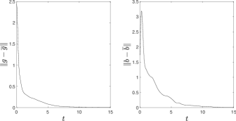
Figure 1: The pose estimation error $\|g(t)-\bar{g}(t)\|$ and the velocity bias estimation error $\|b-\bar{b}(t)\|$ by the observer (10).

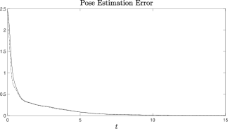
Figure 2: Two pose estimation errors by the observer (10): $\|g(t)-\bar{g}(t)\|$ by the observer (solid) and $\|g(t)-\bar{g}_{\operatorname{SE}(3)}(t)\|$ by the $\operatorname{SE}(3)$ factor $\bar{g}_{\operatorname{SE}(3)}(t)$ of $\bar{g}(t)$ obtained through the projection (21) (dash-dot).

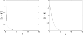
Figure 3: The pose estimation error $\|g(t)-\bar{g}(t)\|$ and the velocity bias estimation error $\|b-\bar{b}(t)\|$ by the observer (13).

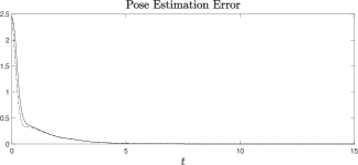
Figure 4: Two pose estimation errors by the observer (13): $\|g(t)-\bar{g}(t)\|$ by the observer (solid) and $\|g(t)-\bar{g}_{\operatorname{SE}(3)}(t)\|$ by the $\operatorname{SE}(3)$ factor $\bar{g}_{\operatorname{SE}(3)}(t)$ of $\bar{g}(t)$ obtained through the projection (21) (dash-dot).

IV Conclusion

We have successfully designed globally exponentially convergent continuous observers for kinematic invariant systems on finite-dimensional matrix Lie groups that estimate state and constant velocity bias from measurements of landmarks, vectors and biased velocity. We have applied the result to the special Euclidean group $\operatorname{SE}(3)$ and carried out a simulation study to illustrate an excellent performance of the observer for $\operatorname{SE}(3)$. We plan to apply the result to drone control [5] and to combine it with deep neural networks [3].

Proof of Theorem II.4

Proof.

From (1) and Assumption II.1, $A(t)$ satisfies

$$\dot{A}=A\xi.$$ (22)

By Assumption II.2, the observer (3) can be written as

$$\dot{\bar{A}} =\bar{A}(\xi+b)-A\bar{b}+k_{P}E_{A},$$ (23a)

$$\dot{\bar{b}} =-k_{I}\operatorname{\pi_{{\mathfrak{g}}}}(A^{T}E_{A}).$$ (23b)

By Assumption II.3, there is a number $\epsilon$ such that

$$0<\epsilon<\min\left\{H,\frac{1}{\|{F}\|U_{g}\sqrt{k_{I}}}\right\},$$

where

$$H=\frac{4(k_{P}-B_{\xi}-B_{b})L_{g}^{2}\lambda_{\min}({F}^{T}{F})}{(4k_{I}L_{g}^{2}\lambda_{\rm min}({F}^{T}{F})+(k_{P}+B_{b}+2B_{\xi})^{2})U_{g}^{2}\|{F}\|^{2}}.$$

The following three quadratic functions of $(\|E_{A}\|,\|e_{b}\|)$ are then all positive definite:

$$V_{1}(\|E_{A}\|,\|e_{b}\|) =\frac{1}{2}\|E_{A}\|^{2}+\frac{1}{2k_{I}}\|e_{b}\|^{2}\!-\!\epsilon U_{g}\|{F}\|\|E_{A}\|\|e_{b}\|,$$

$$V_{2}(\|E_{A}\|,\|e_{b}\|) =\frac{1}{2}\|E_{A}\|^{2}+\frac{1}{2k_{I}}\|e_{b}\|^{2}\!+\!\epsilon U_{g}\|{F}\|\|E_{A}\|\|e_{b}\|,$$

$$V_{3}(\|E_{A}\|,\|e_{b}\|) =(k_{P}-(B_{\xi}+B_{b})-\epsilon k_{I}U_{g}^{2}\|{F}\|^{2})\|E_{A}\|^{2}$$

$$\quad+\epsilon\lambda_{\rm min}({F}^{T}{F})L_{g}^{2}\|e_{b}\|^{2}$$

$$\quad-\epsilon(k_{P}+B_{b}+2B_{\xi})U_{g}\|{F}\|\|E_{A}\|\|e_{b}\|.$$

Hence, there are numbers $\alpha>0$ and $\beta>0$ such that

$$V_{2}\leq\alpha V_{1},\quad\beta V_{2}\leq V_{3}.$$ (24)

Let

$$V(E_{A},e_{b})=\frac{1}{2}\|E_{A}\|^{2}+\frac{1}{2k_{I}}\|e_{b}\|^{2}+\epsilon\langle E_{A},Ae_{b}\rangle,$$

which satisfies

$$V_{1}(\|E_{A}\|,\|e_{b}\|)\leq V(E_{A},e_{b})\leq V_{2}(\|E_{A}\|,\|e_{b}\|)$$ (25)

for all $(E_{A},e_{b})\in\mathbb{R}^{n\times n}\times{\mathfrak{g}}$ by the Cauchy-Schwarz inequality and $\|A\|=\|{F}g\|\leq\|{F}\|U_{g}$. From (22), (23), and the assumption of the bias $b$ being constant, it follows that the estimation error $(E_{A},e_{b})$ obeys

$$\dot{E}_{A} =E_{A}(\xi+b)-Ae_{b}-k_{P}E_{A},$$

$$\dot{e}_{b} =k_{I}\operatorname{\pi_{{\mathfrak{g}}}}(A^{T}E_{A}).$$

Along any trajectory of the composite system consisting of the rigid body (1) and the observer (3),

$$\frac{dV}{dt} =\langle E_{A},E_{A}(\xi+b)-Ae_{b}-k_{P}E_{A}\rangle$$

$$\quad+\langle e_{b},\operatorname{\pi_{{\mathfrak{g}}}}(A^{T}E_{A})\rangle$$

$$\quad+\epsilon\langle E_{A}(\xi+b)-Ae_{b}-k_{P}E_{A},Ae_{b}\rangle$$

$$\quad+\epsilon\langle E_{A},A\xi e_{b}\rangle+\epsilon k_{I}\langle E_{A},A\operatorname{\pi_{{\mathfrak{g}}}}(A^{T}E_{A})\rangle$$

$$\leq-(k_{P}-(B_{\xi}+B_{b})-\epsilon k_{I}U_{g}^{2}\|{F}\|^{2})\|E_{A}\|^{2}$$

$$\quad-\epsilon\lambda_{\rm min}({F}^{T}{F})L_{g}^{2}\|e_{b}\|^{2}$$

$$\quad+\epsilon(k_{P}+B_{b}+2B_{\xi})U_{g}\|{F}\|\|E_{A}\|\|e_{b}\|$$

$$=-V_{3}\leq-\beta V_{2}\leq-\beta V,$$

where the following have been used:

$$\langle E_{A},E_{A}(\xi+b)\rangle\leq\|E_{A}\|^{2}(B_{\xi}+B_{b}),$$

$$\langle E_{A},Ae_{b}\rangle=\langle A^{T}E_{A},e_{b}\rangle=\langle\operatorname{\pi_{{\mathfrak{g}}}}(A^{T}E_{A}),e_{b}\rangle,$$

$$\langle Ae_{b},Ae_{b}\rangle\geq\lambda_{\rm min}({F}^{T}{F})\|ge_{b}\|^{2}\geq\lambda_{\rm min}({F}^{T}{F})L_{g}^{2}\|e_{b}\|^{2},$$

$$\langle E_{A},A\operatorname{\pi_{{\mathfrak{g}}}}(A^{T}E_{A})\rangle=\|\operatorname{\pi_{{\mathfrak{g}}}}(A^{T}E_{A})\|^{2}$$

$$\qquad\qquad\qquad\qquad\quad\leq\|A^{T}E_{A}\|^{2}\leq U_{g}^{2}\|{F}\|^{2}\|E_{A}\|^{2}.$$

Hence, $V(t)\leq V(0)e^{-\beta t}$ for all $t\geq 0$ and all $(\bar{A}(0),\bar{b}(0))\in\mathbb{R}^{n\times n}\times{\mathfrak{g}}$. It follows from (24) and (25) that

$$V_{1}(t)\leq V(t)\leq V(0)e^{-\beta t}\leq V_{2}(0)e^{-\beta t}\leq\alpha V_{1}(0)e^{-\beta t}$$

for all $t\geq 0$ and all $(\bar{A}(0),\bar{b}(0))\in\mathbb{R}^{n\times n}\times{\mathfrak{g}}$. Since $0<\epsilon<1/(\|{F}\|U_{g}\sqrt{k_{I}})$, the map defined by

$$(x_{1},x_{2})\mapsto\sqrt{\frac{1}{2}x_{1}^{2}+\frac{1}{2k_{I}}x_{2}^{2}-\epsilon U_{g}\|{F}\|x_{1}x_{2}}$$

is a norm on $\mathbb{R}^{2}$, where $(x_{1},x_{2})\in\mathbb{R}^{2}$, which is equivalent to the 1-norm on $\mathbb{R}^{2}$ since all norms are equivalent on a finite-dimensional vector space. Hence, $V_{1}(t)\leq\alpha V_{1}(0)e^{-\beta t}$ implies that there exists $C>0$ such that (4) holds for all $t\geq 0$ and all $(\bar{A}(0),\bar{b}(0))\in\mathbb{R}^{n\times n}\times{\mathfrak{g}}$, where $a=\beta/2$. ∎

Proof of Theorem II.10

Proof.

By Assumption II.3, there is a number $\epsilon$ such that

$$0<\epsilon<\min\left\{H,\frac{L_{g}}{\|{F}\|\sqrt{k_{I}}}\right\},$$

where

$$H=\frac{4(k_{P}-B_{\xi}-B_{b})L_{g}^{2}\lambda_{\min}({F}^{T}{F})}{(4k_{I}\lambda_{\rm min}({F}^{T}{F})+(k_{P}+B_{b}+2B_{\xi})^{2}U_{g}^{2})\|{F}\|^{2}}.$$

The following three quadratic functions of $(\|E_{A}\|,\|e_{b}\|)$ are then all positive definite:

$$V_{1}(\|E_{A}\|,\|e_{b}\|) =\frac{1}{2}\|E_{A}\|^{2}+\frac{1}{2k_{I}}\|e_{b}\|^{2}\!-\!\frac{\epsilon}{L_{g}}\|{F}\|\|E_{A}\|\|e_{b}\|,$$

$$V_{2}(\|E_{A}\|,\|e_{b}\|) =\frac{1}{2}\|E_{A}\|^{2}+\frac{1}{2k_{I}}\|e_{b}\|^{2}\!+\!\frac{\epsilon}{L_{g}}\|{F}\|\|E_{A}\|\|e_{b}\|,$$

$$V_{3}(\|E_{A}\|,\|e_{b}\|) =\left(k_{P}-(B_{\xi}+B_{b})-\frac{\epsilon k_{I}\|{F}\|^{2}}{L_{g}^{2}}\right)\|E_{A}\|^{2}$$

$$\quad+\frac{\epsilon\lambda_{\rm min}({F}^{T}{F})}{U_{g}^{2}}\|e_{b}\|^{2}$$

$$\quad-\frac{\epsilon(k_{P}+B_{b}+2B_{\xi})}{L_{g}}\|{F}\|\|E_{A}\|\|e_{b}\|.$$

Hence, there are numbers $\alpha>0$ and $\beta>0$ such that (24) holds. Let

$$V(E_{A},e_{b})=\frac{1}{2}\|E_{A}\|^{2}+\frac{1}{2k_{I}}\|e_{b}\|^{2}-\epsilon\langle E_{A},e_{b}A\rangle,$$

which satisfies (25). Since $b$ is constant by assumption, it follows from (9) and (10) that

$$\dot{E}_{A} =-\xi_{\rm m}E_{A}+e_{b}A-k_{P}E_{A},$$

$$\dot{e}_{b} =-k_{I}\operatorname{\pi_{{\mathfrak{g}}}}(E_{A}A^{T}).$$

Along any trajectory of the composite system consisting of the rigid body (1) and the observer (10),

$$\frac{dV}{dt} =\langle E_{A},-\xi_{\rm m}E_{A}+e_{b}A-k_{P}E_{A}\rangle-\langle e_{b},\operatorname{\pi_{{\mathfrak{g}}}}(E_{A}A^{T})\rangle$$

$$\quad-\epsilon\langle-\xi_{\rm m}E_{A}+e_{b}A-k_{P}E_{A},e_{b}A\rangle$$

$$\quad+\epsilon\langle E_{A},e_{b}\xi A\rangle+\epsilon k_{I}\langle E_{A},\operatorname{\pi_{{\mathfrak{g}}}}(E_{A}A^{T})A\rangle$$

$$\leq-\left(k_{P}-(B_{\xi}+B_{b})-\frac{\epsilon k_{I}\|{F}\|^{2}}{L_{g}^{2}}\right)\|E_{A}\|^{2}$$

$$\quad-\frac{\epsilon\lambda_{\rm min}({F}^{T}{F})}{U_{g}^{2}}\|e_{b}\|^{2}$$

$$\quad+\frac{\epsilon(k_{P}+B_{b}+2B_{\xi})\|{F}\|}{L_{g}}\|E_{A}\|\|e_{b}\|$$

$$=-V_{3}\leq-\beta V_{2}\leq-\beta V.$$

The rest of the proof is identical to the corresponding part in the proof of Theorem II.4, so it is omitted. ∎

Proof of Theorem II.15

Proof.

The measured matrix $A={F}g$ obeys (22) Let

$$\mathcal{E}_{A}=I-A^{-1}\bar{A},\quad e_{b}=b-\bar{b}.$$

From (22) and (12),

$$\dot{\mathcal{E}}_{A} ={\mathcal{E}}_{A}\xi_{\rm m}-\xi{\mathcal{E}}_{A}-e_{b}-k_{P}{\mathcal{E}}_{A}$$

$$\dot{e}_{b} =k_{I}\operatorname{\pi_{{\mathfrak{g}}}}({\mathcal{E}}_{A}).$$

There is an $\epsilon>0$ such that

$$0<\epsilon<\min\left\{\frac{1}{\sqrt{k_{I}}},\frac{4(k_{P}-2B_{\xi}-B_{b})}{4k_{I}+(k_{P}+2B_{\xi}+B_{b})^{2}}\right\}.$$

The following three quadratic functions of $(\|E_{A}\|,\|e_{b}\|)$ are then all positive definite:

$$V_{1}(\|\mathcal{E}_{A}\|,\|e_{b}\|) =\frac{1}{2}\|\mathcal{E}_{A}\|^{2}+\frac{1}{2k_{I}}\|e_{b}\|^{2}\!-\!\epsilon\|\mathcal{E}_{A}\|\|e_{b}\|,$$

$$V_{2}(\|\mathcal{E}_{A}\|,\|e_{b}\|) =\frac{1}{2}\|\mathcal{E}_{A}\|^{2}+\frac{1}{2k_{I}}\|e_{b}\|^{2}\!+\!\epsilon\|\mathcal{E}_{A}\|\|e_{b}\|,$$

$$V_{3}(\|\mathcal{E}_{A}\|,\|e_{b}\|) =(k_{P}-(2B_{\xi}+B_{b})-\epsilon k_{I})\|\mathcal{E}_{A}\|^{2}$$

$$\quad+\epsilon\|e_{b}\|^{2}-\epsilon(k_{P}+B_{b}+2B_{\xi})\|E_{A}\|\|e_{b}\|.$$

Hence, there are numbers $\alpha>0$ and $\beta>0$ such that (24) holds. Let

$$V(\mathcal{E}_{A},e_{b})=\frac{1}{2}\|\mathcal{E}_{A}\|^{2}+\frac{1}{2k_{I}}\|e_{b}\|^{2}+\epsilon\langle\mathcal{E}_{A},e_{b}\rangle,$$

which satisfies (25) for all $(\mathcal{E}_{A},e_{b})\in\mathbb{R}^{n\times n}\times{\mathfrak{g}}$. It is easy to show that along any trajectory of the composite system consisting of the rigid body (1) and the observer (12),

$$\dot{V}\leq-V_{3}\leq-\beta V_{2}\leq-\beta V.$$

As in the proof of Theorem II.4, it is east to show that there are numbers $\tilde{C}>0$ and $a>0$ such that

$$\|{\mathcal{E}}_{A}(t)\|+\|e_{b}(t)\|\leq\tilde{C}(\|{\mathcal{E}}_{A}(0)\|+\|e_{b}(0)\|)e^{-at}$$ (26)

for all $(\bar{A}(0),\bar{b}(0))\in\mathbb{R}^{n\times n}\times{\mathfrak{g}}$ and all $t\geq 0$. Since ${\mathcal{E}}_{A}=I-A^{-1}\bar{A}=A^{-1}E_{A}$ or $E_{A}=A{\mathcal{E}}_{A}={F}g{\mathcal{E}}_{A}$, we have

$$\sigma_{\rm min}({F})L_{g}\|{\mathcal{E}}_{A}\|\leq\|E_{A}\|\leq\sigma_{\rm max}({F})U_{g}\|{\mathcal{E}}_{A}\|.$$ (27)

It follows from (26) and (27) that there is a number $C>0$ such that

$$\|E_{A}(t)\|+\|e_{b}(t)\|\leq C(\|E_{A}(0)\|+\|e_{b}(0)\|)e^{-at}$$

for all $(\bar{A}(0),\bar{b}(0))\in\mathbb{R}^{n\times n}\times{\mathfrak{g}}$ and all $t\geq 0$. ∎

References

• [1] P. Batista, C. Silvestre, and P. Oliveira, “Globally exponentially stable cascade observers for attitude estimation,” Control Engineering Practice, 20, 148 – 155, 2012.
• [2] A.M. Bloch, Nonholonomic Mechanics and Control, Springer, 2003.
• [3] A.L. Caterini and D.E. Chang, Deep Neural Networks in a Mathematical Framework, Springer, 2018.
• [4] D.E. Chang, “On controller design for systems on manifolds in Euclidean space,” Journal on Robust and Nonlinear Control, 28(16), 4981 – 4998, 2018.
• [5] D.E. Chang and Y. Eun, “Global chartwise feedback linearization of the quadcopter with a thrust positivity preserving dynamic extension,” IEEE Trans. Automatic Control, 62 (9), 4747 – 4752, 2017.
• [6] F.A. Goodarzi and T. Lee, “Global formulation of an extended Kalman filter on SE(3) for geometric control of a quadrotor UAV,” J Intell Robot Syst, 88, 395 – 413, 2017.
• [7] M.-D. Hua, T. Hamel, R. Mahony and J. Trumpf, “Gradient-like observer design on the special Euclidean group SE(3) with system outputs on the real projective space,” In Proc. 54th IEEE Conference on Decision and Control, 2139 – 2145, Osaka Japan, 2015.
• [8] A. Khosravian, J. Trumpf, R. Mahony, and C. Lageman, “Bias estimation for invariant systems on Lie groups with homogeneous outputs,” In Proc. IEEE Conf. on Decision and Control, 4454 – 4460, Florence, Italy, December 2013.
• [9] A. Khosravian, J. Trumpf, R. Mahony, and C. Lageman, “Observers for invariant systems on Lie groups with biased input measurements and homogeneous outputs,” Automatica, 55, 19 – 26, 2015.
• [10] C. Lageman, J. Trumpf, and R. Mahony, “Gradient-like observers for invariant dynamics on a Lie group,” IEEE Transactions on Automatic Control, 55(2), 367–377, 2010.
• [11] P. Martin and I. Sarras, “A global observer for attitude and gyro biases from vector measurements,” IFAC PapersOnLine, 50-1, 15409 – 15415, 2017.
• [12] M. Wang and A. Tayebi, “On the design of hybrid pose and velocity-bias observers on Lie group SE(3),” 2018, arXiv Preprint arXiv:1805.00897.
• [13] J.F. Vasconcelos, R. Cunha, C. Silvestre, and P. Oliveira. “A nonlinear position and attitude observer on SE(3) using landmark measurements,” Systems & Control Letters, 59 (3-4), 155 – 166, 2010.