Asynchronous decentralized successive convex approximation

Abstract

We study decentralized asynchronous multiagent optimization over networks, modeled as directed graphs. The optimization problem consists of minimizing a (nonconvex) smooth function–the sum of the agents’ local costs–plus a convex (nonsmooth) regularizer, subject to convex constraints. Agents can perform their local computations as well as communicate with their immediate neighbors at any time, without any form of coordination or centralized scheduling; furthermore, when solving their local subproblems, they can use outdated information from their neighbors. We propose the first distributed algorithm, termed ASY-DSCA, working in such a general asynchronous scenario and applicable to constrained, composite optimization. When the objective function is nonconvex, ASY-DSCA is proved to converge to a stationary solution of the problem at a sublinear rate. When the problem is convex and satisfies the Luo-Tseng error bound condition, ASY-DSCA converges at an R-linear rate to the optimal solution. Luo-Tseng (LT) condition is weaker than strong convexity of the objective function, and it is satisfied by several nonstrongly convex functions arising from machine learning applications; examples include LASSO and logistic regression problems. ASY-DSCA is the first distributed algorithm provably achieving linear rate for such a class of problems.

1 Introduction

We consider the following general class of (possibly nonconvex) multiagent composite optimization:

$$\min_{x\in\mathcal{K}}U(x)\triangleq\sum_{i\in[I]}f_{i}(x)+G(x),\vspace{-0.2cm}$$ (P)

where $[I]\triangleq\{1,\ldots,I\}$ is the set of agents in the system, $f_{i}:\mathbb{R}^{n}\to\mathbb{R}$ is the cost function of agent $i$, assumed to be smooth but possibly nonconvex; $G:\mathbb{R}^{n}\to\mathbb{R}$ is convex possibly nonsmooth; and $\mathcal{K}\subseteq\mathbb{R}^{n}$ is a closed convex set. Each agent has access only to its own objective $f_{i}$ but not the sum $\sum_{i=1}^{I}f_{i}$ while $G$ and $\mathcal{K}$ are common to all the agents.

Problem (P) has found a wide range of applications in machine learning, particularly in supervised learning; examples include logistic regression, SVM and LASSO, and deep learning. In these problems, each $f_{i}$ is the empirical risk that measures the mismatch between the model (parameterized by $x$) to be learnt, and the data set owned only by agent $i$. $G$ and $\mathcal{K}$ plays the role of regularization that restricts the solution space to promote some favorable structure, such as sparsity.

Classic distributed learning typically subsumes a master-slave computational architecture wherein the master nodes run the optimization algorithm gathering the needed information from the workers (cf. Fig. 1-left panel). In contrast, in this paper, we consider a decentralized computational architecture, modeled as a general directed graph that lacks a central controller/master node (see Fig. 1-right panel). Each node can only communicate with its intermediate neighbors. This setting arises naturally when data are acquired and/or stored at the node sides. Examples include resource allocation, swarm robotic control, and multi-agent reinforcement learning [littman1994markov, zhang2018fully]. Furthermore, in scenarios where both architectures are available, decentralized learning has the advantage of being robust to single point failures and being communication efficient. For instance, [lian2017can] compared the performance of stochastic gradient descent on both architectures; they show that, the two implementations have similar total computational complexity, while the maximal communication cost per node of the algorithm running on the decentralized architecture is $\mathcal{O}(\text{degree of network})$, significantly smaller than the $\mathcal{O}(I)$ of the same scheme running on a master-slave system.

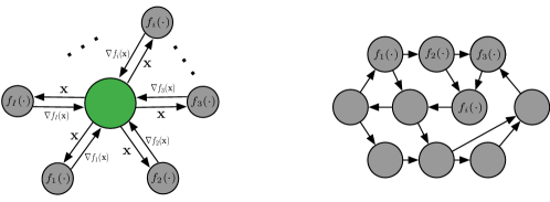
Figure 1: Master-slave (left panel) vs. decentralized (right panel) architectures.

As the problem and network size scale, synchronizing the entire multiagent system becomes inefficient or infeasible. Synchronous schedules require a global clock, which is against the gist of removing the central controller as in decentralized optimization. This calls for the development of asynchronous decentralized learning algorithms. In addition, asynchronous modus operandi brings also benefits such as mitigating communication and/or memory-access congestion, saving resources (e.g., energy, computation, bandwidth), and making algorithms more fault-tolerant. Therefore, asynchronous decentralized algorithms have the potential to prevail in large scale learning problems. In this paper, we consider the following general decentralized asynchronous setting:

(i)

Agents can perform their local computations as well as communicate (possibly in parallel) with their immediate neighbors at any time, without any form of coordination or centralized scheduling; and

(ii)

when solving their local subproblems, they can use outdated information from their neighbors, subject to arbitrary but bounded delays.

We are not aware of any provably convergence scheme applicable to the envisioned decentralized asynchronous setting and Problem (P)–specifically in the presence of constraints or the nonsmooth term $G$–see Sec. 1.2 for a discussion of related works. This paper fills exactly this gap.

1.1 Main contributions

Our major contributions are summarized next.

$\bullet$ Algorithmic design: We introduce ASY-DSCA, the first distributed asynchronous algorithm [in the sense (i) and (ii) above] applicable to the composite, constrained optimization (P). ASY-DSCA builds on successive convex approximation techniques (SCA) [facchinei2015parallel, Scutari_Ying_LectureNote, scutari_PartI, scutari_PartII]–agents solve strongly convex approximations of (P)–coupled with a suitably defined perturbed push-sum mechanism that is robust against asynchrony, whose goal is to track locally and asynchronously the average of agents’ gradients. No specific activation mechanism for the agents’ updates, coordination, or communication protocol is assumed, but only some mild conditions ensuring that information used in the updates does not become infinitely old. We remark that SCA offers a unified umbrella to deal efficiently with convex and nonconvex problems [facchinei2015parallel, Scutari_Ying_LectureNote, scutari_PartI, scutari_PartII]: for several problems (P) of practical interest (cf. Sec. 2.1), a proper choice of the agents’ surrogate functions to minimize leads to subproblems that admit a closed form solution (e.g., soft-thresholding and/or projection to the Euclidean ball). ASY-DSCA generalizes ASY-SONATA, proposed in the companion paper [Tian_arxiv], by i) enabling SCA models in the agents’ local updates; and ii) enlarging the class of optimization problems to include constraints and nonsmooth (convex) objectives.

$\bullet$ Convergence rate: Our convergence results are the following: i) For general nonconvex $F$ in (P), a sublinear rate is established for a suitably defined merit function measuring both distance of the (average) iterates from stationary solutions and consensus disagrement; ii) When (P) satisfies the Luo-Tseng (LT) error bound condition [luo1993error], we establish R-linear convergence of the sequence generated by ASY-DSCA to an optimal solution. Notice that the LT condition is weaker than strong convexity, which is the common assumption used in the literature to establish linear convergence of distributed (even synchronous) algorithms. Our interest in the LT condition is motivated by the fact that several popular objective functions arising from machine learning applications are nonstrongly convex but satisfy the LT error bound; examples include popular empirical losses in high-dimensional statistics such as quadratic and logistic losses–see Sec.2.2 for more details. ASY-DSCA is the first asynchronous distributed algorithm with provably linear rate for such a class of problems over networks; this result is new even in the synchronous distributed setting.

$\bullet$ New line of analysis: We put forth novel convergence proofs, whose main novelties are highlighted next.

1.1.1 New Lyapunov function for descent

Our convergence analysis consists in carefully analyzing the interaction among the consensus, the gradient tracking and the nonconvex-nonsmooth-constrained optimization processes in the asynchronous environment. This interaction can be seen as a perturbation that each of these processes induces on the dynamics of the others. The challenge is proving that the perturbation generated by one system on the others is of a sufficiently small order (with respect to suitably defined metrics), so that convergence can be established and a convergence rate of suitably defined quantities be derived. Current techniques from centralized (nonsmooth) SCA optimization methods [facchinei2015parallel, Scutari_Ying_LectureNote, scutari_PartI, scutari_PartII], error-bound analysis [luo1993error], and (asynchronous) consensus algorithms, alone or brute-forcely put together, do not provide a satisfactory answer: they would generate “too large” perturbation errors and do not exploit the interactions among different processes. On the other hand, existing approaches proposed for distributed algorithms are not applicable too (see Sec. 1.2 for a detailed review of the state of the art): they can neither deal with asynchrony (e.g., [sun2019convergence]) or be applicable to optimization problems with a nonsmooth function in the objective and/or constraints.

To cope with the above challenges our analysis builds on two new Lyapunov functions, one for nonconvex instances of (P) and one for convex ones. These functions are carefully crafted to combine objective value dynamics with consensus and gradient errors while accounting for asynchrony and outdated information in the agents’ updates. Apart from the specific expression of these functions, a major novelty here is the use in the Lyapunov functions of weighting vectors that endogenously vary based upon the asynchrony trajectory of the algorithm–see Sec.6 (Step 2) and Sec.7 (Remark 17) for technical details. The descent property of the Lyapunov functions is the key step to prove that consensus and tracking errors vanish and further establish the desired converge rate of valid optimality/stationarity measures.

1.1.2 Linear rate under the LT condition

The proof of linear convergence of ASY-DSCA under the LT condition is a new contribution of this work. Existing proofs establishing linear rate of distributed synchronous and asynchronous algorithms [shi2015extra, Nedich-geometric, qu2017harnessing, sun2019convergence, alghunaim2019decentralized] (including our companion paper [Tian_arxiv]) are not applicable here, as they all leverage strong convexity of $F$, a property that we do not assume. On the other hand, existing techniques showing linear rate of centralized first-order methods under the LT condition [luo1993error, tseng1991rate] do not customize to our distributed, asynchronous setting. Roughly speaking, this is mainly due to the fact that use of the LT condition in [luo1993error, tseng1991rate] is subject to proving descent on the objective function along the algorithm iterates, a property that can no longer be guaranteed in the distributed setting, due to the perturbations generated by the consensus and the gradient tracking errors. Asynchrony complicates further the analysis, as it induces unbalanced updating frequency of agents and the presence of the outdated information in agents’ local computation. Our proof of linear convergence leverages the descent property of the proposed Lyapunov function to be able to invoke the LT condition in our distributed, asynchronous setting (see Sec.6 for a technical discussion on this matter).

1.2 Related works

On the asynchronous model: The literature on asynchronous methods is vast; based upon agents’ activation rules and assumptions on delays, existing algorithms can be roughly grouped in three categories. 1) Algorithms in [wang2015cooperative, li2016distributed, Tsianos:ef, Tsianos:en, lin2016distributed, doan2017impact] tolerate delayed information but require synchronization among agents, thus fail to meet the asynchronous requirement (i) above. 2) On the other hand, schemes in [NotarnicolaNotarstefanoTAC17, xu2017convergence, iutzeler2013asynchronous, wei20131, bianchi2016coordinate, hendrikx2019asynchronous, hendrikx2018accelerated] accounts for agents’ random (thus uncoordinated) activation; however, upon activation, they must use the most updated information from their neighbors, i.e., no delays are allowed; hence, they fail to meet requirement (ii). 3) Asynchronous activations and delays are considered in  [nedic2011asynchronous, zhao2015asynchronous, kumar2017asynchronous, peng2016arock, wu2016decentralized] and [eisen2017decentralized, bof2017newton, Tian_arxiv, olshevsky2018robust, assran2018asynchronous], with the former (resp. latter) schemes employing random (resp. deterministic) activations. Some restrictions on the form of delays are imposed. Specifically, [nedic2011asynchronous, zhao2015asynchronous, kumar2017asynchronous, bof2017newton] can only tolerate packet losses (either the information gets lost or is received with no delay); [assran2018asynchronous] handles only communication delays (eventually all the transmitted information is received by the intended agent); and [peng2016arock, wu2016decentralized] assume that the agents’ activation and delay as independent random variables, which is not realistic and hard to enforce in practice [cannelli2016asynchronous].

The only schemes we are aware of that are compliant with the asynchronous model (i) and (ii) are those in [Tian_arxiv, olshevsky2018robust]; however, they are applicable only to smooth unconstrained problems. Furthermore, all the aforementioned algorithms but [kumar2017asynchronous, Tian_arxiv] are designed only for convex objectives $U$.

On the convergence rate: Referring to convergence rate guarantees, none of the aforementioned methods is proved to converge linearly in the asynchronous setting and when applied to nonsmooth constrained problems in the form (P). Furthermore, even restricting the focus to synchronous distributed methods or smooth unconstrained instances of (P), we are not aware of any distributed scheme that provably achieves linear rate without requiring $U$ to be strongly convex; we refer to [sun2019convergence] for a recent literature review of synchronous distributed schemes belonging to this class. In the centralized setting, linear rate can be proved for first order methods under the assumption that $U$ satisfies some error bound conditions, which are weaker than strongly convexity; see, e.g., [zhang2013linear, bolte2017error, luo1993error, karimi2016linear]. A natural question is whether such results can be extended to (asynchronous) decentralized methods. This paper provides a positive answer to this open question.

1.3 Notation

The $i$-th vector of the standard basis in $\mathbb{R}^{n}$ is denoted by $e_{i}$; $x_{i}$ is the $i$-th entry of a vector $x$; and $A_{i}$ denotes the $i$-th row of a matrix $A$. Given two matrices (vectors) $A$ and $B$ of same size, by $A\preccurlyeq B$ we mean that $B-A$ is a nonnegative matrix (vector). We do not differentiate between a vector and its transpose when it is the argument of a function/mapping. The vector of all ones is denoted by $\mathbf{1}$ (its dimension will be clear from the context). We use $\left\lVert\cdot\right\rVert$ to denote the Frobenius norm when the argument is a matrix and the Euclidean norm when applied to a vector; $\left\lVert\cdot\right\rVert_{2}$ denotes the spectral norm of a matrix. Given $G:\mathbb{R}^{n}\to\mathbb{R}$, the proximal mapping is defined as $\text{prox}_{G}(x)\triangleq\mathop{\rm argmin}_{y\in\mathcal{K}}G(y)+\frac{1}{2}\left\lVert y-x\right\rVert_{2}^{2}$. Let $\mathcal{K}^{*}$ denote the set of stationary solutions of (P), and $\text{dist}(x,\mathcal{K}^{*})\triangleq\min_{y\in\mathcal{K}^{*}}\|x-y\|$.

2 Problem setup

We study Problem (P) under the following assumptions.

Assumption 1 (On Problem (P)).

The following hold:

(i) The set $\mathcal{K}\subset\mathbb{R}^{n}$ is nonempty, closed, and convex;

(ii) Each $f_{i}:\mathcal{O}\rightarrow\mathbb{R}$ is proper, closed and $l$-smooth, where $\mathcal{O}\supset\mathcal{K}$ is open; $F$ is $L$-smooth with $L\triangleq I\cdot l$;

(iii) $G:\mathcal{K}\to\mathbb{R}$ is convex but possibly nonsmooth; and  (iv) $U$ is lower bounded on $\mathcal{K}$.

Note that each $f_{i}$ need not be convex, and each agent $i$ knows only its own $f_{i}$ but not $\sum_{j\neq i}f_{j}$. The regularizer $G$ and the constraint set $\mathcal{K}$ are common knowledge to all agents.

To solve Problem (P), agents need to leverage message exchanging over the network. The communication network of the agents is modeled as a fixed, directed graph $\mathcal{G}\triangleq(\mathcal{V},\mathcal{E})$. $\mathcal{V}\triangleq[I]$ is the set of nodes (agents), and $\mathcal{E}\subseteq\mathcal{V}\times\mathcal{V}$ is the set of edges (communication links). If $(i,j)\in\mathcal{E}$, it means that agent $i$ can send information to agent $j$. We assume that the digraph does not have self-loops. We denote by $\mathcal{N}_{i}^{in}$ the set of in-neighbors of agent $i$, i.e., $\mathcal{N}_{i}^{in}\triangleq\left\{j\in\mathcal{V}\mid(j,i)\in\mathcal{E}\right\}$ while $\mathcal{N}_{i}^{out}\triangleq\left\{j\in\mathcal{V}\mid(i,j)\in\mathcal{E}\right\}$ is the set of its out-neighbors. The following assumption on the graph connectivity is standard.

Assumption 2.

The graph $\mathcal{G}$ is strongly connected.

2.1 Case study: Collaborative supervised learning

A timely application of the described decentralized setting and optimization Problem (P) is collaborative supervised learning. Consider a training data set $\{\left(u_{s},y_{s}\right)\}_{s\in\mathcal{D}}$, where $u_{s}$ is the input feature vector and $y_{s}$ is the outcome associated to item $s.$ In the envisioned decentralized setting, data $\mathcal{D}$ are partitioned into $I$ subsets $\{\mathcal{D}_{i}\}_{i\in[I]}$, each of which belongs to an agent $i\in[I]$. The goal is to learn a mapping $p(\cdot\,;x)$ parameterized by $x\in\mathbb{R}^{n}$ using all samples in $\mathcal{D}$ by solving $\min_{x\in\mathcal{K}}{1}/{|\mathcal{D}|}\sum_{s\in\mathcal{D}}\ell\left(p(u_{s};x),y_{s}\right)+G(x),$ wherein $\ell$ is a loss function that measures the mismatch between $p(u_{s};x)$ and $y_{s}$; and $G$ and $\mathcal{K}$ play the role of regularizing the solution. This problem is an instance of (P) with $f_{i}(x)\triangleq{1}/{|\mathcal{D}|}\sum_{s\in\mathcal{D}_{i}}\ell\left(p(u_{s};x),y_{s}\right)$. Specific examples of loss functions and regularizers are give next.

1. Elastic net regularization for log linear models: $\ell\left(p(u_{s};x),y_{s}\right)\triangleq\Phi(u_{s}^{\top}x)-y_{s}\cdot(u_{s}^{\top}x)$ with $\Phi$ convex, $u_{s}\in\mathbb{R}^{n}$ and $y_{s}\in\mathbb{R}$; $G(x)\triangleq\lambda_{1}\left\lVert x\right\rVert_{1}+\lambda_{2}\left\lVert x\right\rVert_{2}^{2}$ is the elastic net regularizer, which reduces to the LASSO regularizer when $(\lambda_{1},\lambda_{2})=(\lambda,0)$ or the ridge regression regularizer when $(\lambda_{1},\lambda_{2})=(0,\lambda)$;

2. Sparse group LASSO [friedman2010note]: The loss function is the same as that in example 1), with $\Phi(t)=t^{2}/2$; $G(x)=\sum_{S\in\mathcal{J}}w_{S}\left\lVert x_{S}\right\rVert_{2}+\lambda\left\lVert x\right\rVert_{1}$, where $\mathcal{J}$ is a partition of $[n]$;

3. Logistic regression: $\ell\left(p(u_{s};x),y_{s}\right)\triangleq\text{ln}(1+e^{-y_{s}\cdot u_{s}^{\top}x})$; popular choices of $G(x)$ are $G(x)\triangleq\lambda\left\lVert x\right\rVert_{1}$ or $G(x)\triangleq\lambda\left\lVert x\right\rVert_{2}^{2}$. The constraint set $\mathcal{K}$ is generally assumed to be bounded.

For large scale data sets, solving such learning problems is computationally challenging even if $F$ is convex. When the problem dimension $n$ is larger than the sample size $|\mathcal{D}|$, the Hessian of the empirical risk loss $F$ is typically rank deficient and hence $F$ is not strongly convex. Since linear convergence rate for decentralized methods is established in the literature only under strong convexity, it is unclear whether such a fast rate can be achieved under less restrictive conditions, e.g., embracing popular high-dimensional learning problems as those mentioned above. We show next that a positive answer to this question can be obtained leveraging the renowned LT error bound, a condition that has been wide explored in the literature of centralized optimization methods.

2.2 The Luo-Tseng error bound

Assumption 3.

(Error-bound conditions [Dembo1984local, pang1986inexact, luo1993error]):

(i)

$F$ is convex;

(ii)

For any $\eta\!>\!\inf_{x\in\mathcal{K}}\!U(x)$, there exists $\epsilon,\kappa>0$ such that:

$$U(x)\leq\eta\quad\text{and}\quad\left\lVert x-\text{prox}_{G}(x-\nabla F(x))\right\rVert\leq\epsilon\vspace{-0.5cm}$$ (1)

$$\Downarrow\vspace{-0.4cm}$$

$$\text{dist}(x,\mathcal{K}^{*})\leq\kappa\left\lVert x-\text{prox}_{G}(x-\nabla F(x))\right\rVert.$$ (2)

Assumption 3(ii) is a local growth condition on $U$ around $\mathcal{K}^{*}$, crucial to prove linear rate. Note that for convex $F$, condition 3(ii) is equivalent to other renowned error bound conditions, such as the Polyak-Łojasiewicz [polyak1964gradient, lojasiewicz1963topological], the quadratic growth [drusvyatskiy2018error], and the Kurdyka-Łojasiewicz [bolte2017error] conditions. A broad class of functions satisfying Assumption 3 is in the form $U(x)=F(x)+G(x)$, with $F$ and $G$ such that (cf. [tseng2009coordinate, Theorem 4], [zhang2013linear, Theorem 1]):

(i)

$F(x)=h(Ax)$ is $L$-smooth, where $h$ is strongly convex and $A$ is any linear operator;

(ii)

$G$ is either a polyhedral convex function (i.e., its epigraph is a polyhedral set) or has a specific separable form as $G(x)=\sum_{S\in\mathcal{J}}w_{S}\left\lVert x_{S}\right\rVert_{2}+\lambda\left\lVert x\right\rVert_{1}$, where $\mathcal{J}$ is a partition of the set $[n]$, and $\lambda$ and $w_{S}$’s are nonnegative weights (we used $x_{S}$ to denote the vector whose component $i$ is $x_{i}$ if $i\in S$, and $0$ otherwise);

(iii)

$U(x)$ is coercive.

It follows that all examples listed in Section 2.1 satisfy Assumption 3. Hence, the proposed decentralized asynchronous algorithm, to be introduced, will provably achieve linear rate for such a general classes of problems.

3 Algorithmic development

Solving Problem (P) over $\mathcal{G}$ poses the following challenges: i) $U$ is nonconvex/nonsmooth; ii) each agent $i$ only knows its local loss $f_{i}$ but not the global $F$; and iii) agents perform updates in an asynchronous fashion. Furthermore, it is well established that, when $f_{i}$ are nonconvex (or convex only in some variable), using convex surrogates for $f_{i}$ in the agents’ subproblems rather than just linearization (as in gradient algorithms) provides more flexibility in the algorithmic design and can enhance practical convergence [facchinei2015parallel, Scutari_Ying_LectureNote, scutari_PartI, scutari_PartII]. This motivated us to equip our distributed asynchronous design with SCA models.

To address these challenges, we develop our algorithm building on SONATA [YingMAPR, sun2019convergence], as to our knowledge it is the only synchronous decentralized algorithm for (P) capable to handle challenges i) and ii) and incorporating SCA techniques. Moreover, when employing a constant step size, it converges linearly to the optimal solution of (P) when $F$ is strongly convex; and sublinearly to the set of stationary points of  (P), when $F$ is nonconvex. We begin briefly reviewing SONATA.

3.1 Preliminaries: the SONATA algorithm [YingMAPR, sun2019convergence]

Each agent $i$ maintains a local estimate $x_{i}$ of the common optimization vector $x$, to be updated at each iteration; the $k$-th iterate is denoted by $x_{i}^{k}$. The specific procedure put forth by SONATA is given in Algorithm 1 and briefly described next.

Algorithm 1 The SONATA Algorithm

Data: For all agent $i$ and $\forall j\in\mathcal{N}_{i}^{in}$, $x_{i}^{0}\in\mathbb{R}^{n}$, ${z}_{i}^{0}=y_{i}^{0}=\nabla f_{i}(x_{i}^{0})$, $\phi_{i}^{0}=1$. Set $k=0$.

while a termination criterion is not met, each agent $i\in[I]$ do

     (S.1) Local optimization:

$$\begin{split}&\widetilde{x}_{i}^{k}=\underset{x\in\mathcal{K}}{\mathrm{argmin}}\leavevmode\nobreak\ \big{\{}\widehat{U}_{i}\big{(}x;x_{i}^{k},I\,y_{i}^{k}-\nabla f_{i}(x_{i}^{k})\big{)}\triangleq\\ &\quad\widetilde{f}_{i}(x;x_{i}^{k})+(I\,y_{i}^{k}-\nabla f_{i}(x_{i}^{k}))^{\top}\left(x-x_{i}^{k}\right)+G(x)\big{\}},\end{split}$$ (3a)

$$\begin{split}&v_{i}^{k+1}=x_{i}^{k}+\gamma\left(\widetilde{x}_{i}^{k}-x_{i}^{k}\right).\end{split}$$ (3b)

     (S.2) Consensus step:

$$x_{i}^{k+1}=w_{ii}v_{i}^{k+1}+\sum_{j\in\mathcal{N}_{i}^{{in}}}w_{ij}v_{j}^{k+1}.$$ (4)

     (S.3) Gradient tracking:

$$\begin{split}&z_{i}^{k+1}=\sum_{j=1}^{I}a_{ij}\left(z_{j}^{k}+\nabla f_{j}(x_{j}^{k+1})-\nabla f_{j}(x_{j}^{k})\right),\\ &\phi_{i}^{k+1}=\sum_{j=1}^{I}a_{ij}\phi_{j}^{k},\quad y_{i}^{k+1}=\frac{z_{i}^{k+1}}{\phi_{i}^{k+1}}.\end{split}$$ (5)

     $k\leftarrow k+1$

end while

(S.1): Local optimization. At each iteration $k$, every agent $i$ locally solves a strongly convex approximation of Problem (P) at $x_{i}^{k}$, as given in (LABEL:eq:loc_opt), where $\widetilde{f}_{i}:\mathcal{K}\times\mathcal{K}\to\mathbb{R}$ is a so-called SCA surrogate of $f_{i}$, that is, satisfies Assumption 4 below. The second term in (LABEL:eq:loc_opt), ${(Iy_{i}^{k}-\nabla f_{i}(x_{i}^{k}))}^{\top}\left(x-x_{i}^{k}\right)$, serves as a first order approximation of $\sum_{j\neq i}f_{j}(x)$ unknown to agent $i$, wherein $Iy_{i}^{k}$ tracks the sum gradient $\sum_{j=1}^{I}\nabla f_{j}(x_{i}^{k})$ (see step (S.3)). We then employ a relaxation step (LABEL:eq:relaxation) with step size $\gamma$.

Assumption 4.

$\widetilde{f}_{i}:\mathcal{K}\times\mathcal{K}\to\mathbb{R}$ satisfies:

(i)

$\nabla\widetilde{f}_{i}(x;x)=\nabla f_{i}(x)$ for all $x\in\mathcal{K}$;

(ii)

$\widetilde{f}_{i}(\cdot;y)$ is uniformly strongly convex on $\mathcal{K}$ with constant $\widetilde{\mu}>0$;

(iii)

$\nabla\widetilde{f}_{i}(x;\cdot)$ is uniformly Lipschitz continuous on $\mathcal{K}$ with constant $\widetilde{l}$.

The choice of $\widetilde{f}_{i}$ is quite flexible. For example, one can construct a proximal gradient type update (LABEL:eq:loc_opt) by linearizing $f_{i}$ and adding a proximal term; if $f_{i}$ is a DC function, $\widetilde{f}_{i}$ can retain the convex part of $f_{i}$ while linearizing the nonconvex part. We refer to [facchinei2015parallel, Scutari_Ying_LectureNote, scutari_PartI, scutari_PartII] for more details on the choices of $\widetilde{f}_{i}$, and Sec. 5 for specific examples used in our experiments.

(S.2): Consensus. This steps aims at enforcing consensus on the local variables $x_{i}$ via gossiping. Specifically, after the local optimization step, each agent $i$ performs a consensus update (4) with mixing matrix $W=(w_{ij})_{i,j=1}^{I}$ satisfying the following assumption.

Assumption 5.

The weight matrices ${W}\triangleq(w_{ij})_{i,j=1}^{I}$ and ${A}\triangleq(a_{ij})_{i,j=1}^{I}$ satisfy (we will write ${M}\triangleq(m_{ij})_{i,j=1}^{I}$ to denote either ${A}$ or ${W}$ and $\mathbf{1}\in\mathbb{R}^{I}$ is a vector of all ones):

(i)

$\exists\,\bar{m}>0$ such that: $m_{ii}\geq\bar{m}$, $\forall i\in\mathcal{V}$; $m_{ij}\geq\bar{m}$, for all $(j,i)\in\mathcal{E}$; and $m_{ij}=0$, otherwise;

(ii)

${W}$ is row-stochastic, that is, ${W}\,\mathbf{1}=\mathbf{1}$; and iii) ${A}$ is column-stochastic, that is, ${A}^{\top}\,\mathbf{1}=\mathbf{1}$.

Several choices for $W$ and $A$ are available; see, e.g.,  [sayed2014adaptation]. Note that SONATA uses a row-stochastic matrix $W$ for the consensus update and a column-stochastic matrix $A$ for the gradient tracking. In fact, for general digraph, a doubly stochastic matrix compliant with the graph might not exist while one can always build compliant row or column stochastic matrices. These weights can be determined locally by the agents, e.g., once its in- and out-degree can be estimated.

(S.3): Gradient tracking. This step updates $y_{i}$ by employing a perturbed push-sum algorithm with weight matrix $A$ satisfying Assumption 5. This step aims to track the average gradient $(1/I)\sum_{i=1}^{I}\nabla f_{i}(x_{i})$ via $y_{i}$. In fact, using the column stochasticity of $A$ and applying the telescopic cancellation, one can check that the following holds:

$$\vspace{-0.1cm}\sum_{i=1}^{I}\phi_{i}^{k}=\sum_{i=1}^{I}\phi_{i}^{0}=I,\quad\sum_{i=1}^{I}z_{i}^{k}=\sum_{i=1}^{I}\nabla f_{i}(x_{i}^{k}).\vspace{-0.1cm}$$ (6)

It can be shown that for all $i\in[I]$, $z_{i}^{k}$ and $\phi_{i}^{k}$ converges to $\xi_{i}^{k}\cdot\sum_{i=1}^{I}z_{i}^{k}$ and $\xi_{i}^{k}\cdot\sum_{i=1}^{I}\phi_{i}^{k}$, respectively, for some $\xi_{i}^{k}>0$ [nedic2014distributed]. Hence, $y_{i}^{k}=z_{i}^{k}/\phi_{i}^{k}$ converges to $(1/I)\sum_{i=1}^{I}\nabla f_{i}(x_{i}^{k})$, employing the desired gradient tracking.

Notice that the extension of the gradient tracking to the asynchronous setting is not trivial, as the ratio consensus property discussed above no longer holds if agents naively perform their updates using in  (5) delayed information. In fact, packets sent by an agent, corresponding to the summand in (5), may get lost. This breaks the equalities in (6). Consequently, the ratio $y_{i}^{k}$ cannot correctly track the average gradient. To cope with this issue, our approach is to replace step (S.3) by the asynchronous gradient tracking mechanism developed in [Tian_arxiv].

3.2 Asynchronous decentralized SCA (ASY-DSCA)

We now break the synchronism in SONATA and propose ASY-DSCA (cf. Algorithm 2). All agents update asynchronously and continuously without coordination, possibly using delayed information from their neighbors.

Algorithm 2 The ASY-DSCA Algorithm

Data: For all agent $i$ and $\forall j\in\mathcal{N}_{i}^{\text{in}}$, $x_{i}^{0}\in\mathbb{R}^{n}$, ${z}_{i}^{0}=y_{i}^{0}=\nabla f_{i}(x_{i}^{0})$, $\phi_{i}^{0}=1$, $\tilde{{\rho}}_{ij}^{0}=0$, $\tilde{\sigma}_{ij}^{0}=0$, $\tau_{ij}^{-1}=-D$. And for $t=-D,-D+1,\ldots,0$, ${\rho}_{ij}^{t}=0$, $\sigma_{ij}^{t}=0$, $v_{i}^{t}=0$. Set $k=0$.

while a termination criterion is not met do

     Pick: $\quad(i^{k},{d}^{k})$;

     Set: $\quad\tau_{i^{k}j}^{k}=\max(\tau_{i^{k}j}^{k-1},k-d_{j}^{k}),\quad\forall j\in\mathcal{N}_{i^{k}}^{\text{in}};$

     (S.1) Local optimization:

$$\begin{split}&\widetilde{x}_{i^{k}}^{k}=\underset{x\in\mathcal{K}}{\mathrm{argmin}}\quad\widehat{U}_{i^{k}}\left(\,x;\,x_{i^{k}}^{k},\,I\,y_{i^{k}}^{k}-\nabla f_{i^{k}}(x_{i^{k}}^{k})\right),\\ &v_{i^{k}}^{k+1}=x_{i^{k}}^{k}+\gamma\left(\widetilde{x}_{i^{k}}^{k}-x_{i^{k}}^{k}\right);\end{split}$$ (7)

     (S.2) Consensus step (using delayed information):

$$\qquad x_{i^{k}}^{k+1}=w_{i^{k}i^{k}}v_{i^{k}}^{k+1}+\sum_{j\in\mathcal{N}_{i^{k}}^{\text{in}}}w_{{i^{k}}j}v_{j}^{\tau_{i^{k}j}^{k}};$$ (8)

     (S.3) Robust gradient tracking:

$$\qquad y_{i^{k}}^{k+1} =\mathcal{F}\Big{(}i^{k},\,k,\,(\rho_{i^{k}j}^{\tau_{i^{k}j}^{k}})_{j\in\mathcal{N}_{i^{k}}^{\text{in}}},\,(\sigma_{i^{k}j}^{\tau_{i^{k}j}^{k}})_{j\in\mathcal{N}_{i^{k}}^{\text{in}}},$$ (9)

$$\quad\qquad\nabla f_{i^{k}}(x_{i^{k}}^{k+1})-\nabla f_{i^{k}}(x_{i^{k}}^{k})\Big{)}$$

     Untouched state variables shift to state $k+1$ while keeping the same value; $k\leftarrow k+1.$

end while

procedure $\mathcal{F}$($i,k,(\rho_{ij})_{j\in\mathcal{N}_{i}^{\text{in}}},(\sigma_{ij})_{j\in\mathcal{N}_{i}^{\text{in}}},{\epsilon}$)

     Sum step:

$$z_{i}^{k+\frac{1}{2}}=z_{i}^{k}+\sum_{j\in\mathcal{N}_{i}^{\text{in}}}\left(\rho_{{i}j}-\tilde{\rho}_{ij}^{k}\right)+{\epsilon},$$ (10)

$$\phi_{i}^{k+\frac{1}{2}}=\phi_{i}^{k}+\sum_{j\in\mathcal{N}_{i}^{\text{in}}}\left({\sigma}_{{i}j}-\tilde{\sigma}_{ij}^{k}\right);$$

     Push step:

$$z_{i}^{k+1}=a_{ii}\,z_{i}^{k+\frac{1}{2}},\quad\phi_{i}^{k+1}=a_{ii}\,\phi_{i}^{k+\frac{1}{2}};\quad\forall j\in\mathcal{N}_{i}^{\text{out}},$$ (11)

$$\rho_{j{i}}^{k+1}=\rho_{j{i}}^{k}+a_{j{i}}\,z_{i}^{k+\frac{1}{2}},\quad{\sigma}_{j{i}}^{k+1}={\sigma}_{j{i}}^{k}+a_{j{i}}\,\phi_{i}^{k+\frac{1}{2}};$$

     Mass-Buffer update:

$$\tilde{\rho}_{{i}j}^{k+1}=\rho_{{i}j},\quad\tilde{\sigma}_{{i}j}^{k+1}={\sigma}_{{i}j},{\quad\,\ \forall j\in\mathcal{N}_{i}^{\text{in}}};$$ (12)

     return $\quad z_{i}^{k+1}/\phi_{i}^{k+1}.$

end procedure

More specifically, a global iteration counter $k$, unknown to the agents, is introduced, which increases by $1$ whenever a variable of the multiagent system changes. Let $i^{k}$ be the agent triggering iteration $k\to k+1$; it executes Steps (S1)-(S.3) (no necessarily withih the same activation), as described below.

(S.1): Local optimization. Agent $i^{k}$ solves the strongly convex optimization problem (7) based on the local surrogate $\widehat{U}_{i^{k}}$. It is tacitly assumed that $\widehat{U}_{i^{k}}$ is chosen so that (7) is simple to solve (i.e., the solution can be computed in closed form or efficiently). Given the solution $\widetilde{x}_{i^{k}}^{k}$, $v_{i^{k}}^{k+1}$ is generated.

(S.2): Consensus. Agent $i^{k}$ may receive delayed variables from its in-neighbors $j\in\mathcal{N}_{i^{k}}^{in}$, whose iteration index is $k-d_{j}^{k}$. To perform its update, agent $i^{k}$ first sorts the “age” of all the received variables from agent $j$ since $k=0$, and then picks the most recently generated one. This is implemented maintaining a local counter $\tau_{i^{k}j}$, updated recursively as $\tau_{i^{k}j}^{k}=\max(\tau_{i^{k}j}^{k-1},k-d_{j}^{k})$. Thus, the variable agent $i^{k}$ uses from $j$ has iteration index $\tau_{i^{k}j}^{k}$. Since the consensus algorithm is robust against asynchrony [Tian_arxiv], we simply adopt the update of SONATA [cf. (4)] and replace $v_{j}^{k}$ by its delayed version $v_{j}^{\tau_{i^{k}j}^{k}}$.

(S.3): Robust gradient tracking. As anticipated in Sec. 3.1, the packet loss caused by asynchrony breaks the sum preservation property (6) in SONATA. If treated in the same way as the $x$ variable in (8), $y_{i}$ would fail to track $(1/I)\sum_{i=1}^{I}\nabla f_{i}(x_{i})$. To cope with this issue, we leverage the asynchronous sum-push scheme (P-ASY-SUM-PUSH) introduced in our companion paper [Tian_arxiv] and update the $y$-variable as in (9). Each agent $i$ maintains mass counters $(\rho_{ji},\sigma_{ji})$ associated to $(z_{i},\phi_{i})$ that record the cumulative mass generated by $i$ for $j\in\mathcal{N}_{i}^{out}$ since $k=0$; and transmits $(\rho_{ji},\sigma_{ji})$. In addition, agent $i$ also maintains buffer variables $(\tilde{{\rho}}_{ij},\tilde{\sigma}_{ij})$ to track the latest mass counter $(\rho_{ij},\sigma_{ij})$ from $j\in\mathcal{N}_{i}^{in}$ that has been used in its update. We describe now the update of $z$ and $\rho$; $\phi$ and $\sigma$ follows similar steps. For notation simplicity, let $i=i^{k}$ update. It first performs the sum step (10) using a possibly delayed mass counter $\rho_{ij}^{\tau_{ij}^{k}}$ received from $j$. By computing the difference $\rho_{ij}^{\tau_{ij}^{k}}-\tilde{\rho}_{ij}^{k}$, it collects the sum of the $a_{ij}z_{j}$’s generated by $j$ that it has not yet added. Agent $i$ then sums them together with a gradient correction term (perturbation) $\epsilon=\nabla f_{i}(x_{i}^{k+1})-\nabla f_{i}(x_{i}^{k})$ to its current state variable $z_{i}^{k}$ to form the intermediate mass $z_{i}^{k+\frac{1}{2}}$. Next, in the push step (11), agent $i$ splits $z_{i}^{k+\frac{1}{2}}$, maintaining $a_{ii}z_{i}^{k+\frac{1}{2}}$ for itself and accumulating $a_{ji}z_{i}^{k+\frac{1}{2}}$ to its local mass counter $\rho_{ji}^{k}$, to be transmit to $j\in\mathcal{N}_{i}^{out}$. Since the last mass counter agent $i$ processed is $\rho_{ij}^{\tau_{ij}^{k}}$, it sets $\tilde{\rho}_{ij}=\rho_{ij}^{\tau_{ij}^{k}}$ [cf. (12)]. Finally, it outputs $y_{i}^{k+1}\!=\!{z_{i}^{k+1}}/{\phi_{i}^{k+1}}$.

4 Convergence of ASY-DSCA

We study ASY-DSCA under the asynchronous model below.

Assumption 6 (Asynchronous model).

Suppose:

(i)

$\exists$ $0<T<\infty$ such that $\cup_{t=k}^{k+T-1}i^{t}=\mathcal{V}$, for all $k\in\mathbb{N}_{+}$;

(ii)

$\exists$ $0<D<\infty$ such that $0\leq d_{j}^{k}\leq D$, for all $j\in\mathcal{N}_{i^{k}}^{in}$ and $k\in\mathbb{N}_{+}$.

Assumption 6(i) is an essentially cyclic rule stating that within $T$ iterations all agents will have updated at least once, which guarantees that all of them participate “sufficiently often”. Assumption 6(ii) requires bounded delay–old information must eventually be purged by the system. This asynchronous model is general and imposes no coordination among agents or specific communication/activation protocol–an extensive discussion on specific implementations and communication protocols satisfying Assumption 6 can be found for ASY-SONATA in the companion paper [Tian_arxiv] and apply also to ASY-DSCA; we thus omit here further details.

The convergence of ASY-DSCA is established under two settings, namely: i) convex $F$ and error bound Assumption 3 (cf. Theorem 1); and ii) general nonconvex $F$ (cf. Theorem 2).

Theorem 1 (Linear convergence).

Consider (P) under Assumption  1 and 3, and let $U^{\star}$ denote the optimal function value. Let $\{(x_{i}^{k})_{i=1}^{I}\}_{k\in\mathbb{N}}$ be the sequence generated by Algorithm 2, under Assumption 2, 6, and with weight matrices ${W}$ and ${A}$ satisfying Assumption 5. Then, there exist a constant $\bar{\gamma}_{cvx}>0$ and a solution $x^{\star}$ of (P) such that if $\gamma\leq\bar{\gamma}_{cvx}$, it holds

$$\|U(x_{i}^{k})-U(x^{\star})\|=\mathcal{O}(\lambda^{k}),\quad\|x_{i}^{k}-x^{\star}\|=\mathcal{O}\left((\sqrt{\lambda})^{k}\right),$$

for all $i\in\mathcal{V}$ and some $\lambda\in(0,1)$. ∎

Theorem 1 establishes the first linear convergence result of a distributed (synchronous or asynchronous) algorithm over networks without requiring strong convexity but the weaker LT condition. Linear convergence is achieve on both function values and sequence iterates.

We consider now the nonconvex setting. To measure the progress of ASY-DSCA towards stationarity, we introduce the merit function

$$M_{F}(x^{k})\triangleq\max\big{\{}\|\bar{x}^{k}-\text{prox}_{G}(\bar{x}^{k}-\nabla F(\bar{x}^{k}))\|^{2},\sum_{i=1}^{I}\|x_{i}^{k}-\bar{x}^{k}\|^{2}\big{\}},$$ (13)

where $\bar{x}^{k}\triangleq(1/I)\cdot\sum_{i=1}^{I}x_{i}^{k}$, and $\text{prox}_{G}$ is the prox operator (cf. Sec. 2.2). $M_{F}$ is a valid merit function since it is continuous and $M_{F}(x^{k})=0$ if and only if all the $x_{i}$’s are consensual and stationary. The following theorem shows that $M_{F}(x^{k})$ vanishes at sublinear rate.

Theorem 2 (Sublinear convergence).

Consider (P) under Assumption 1 (thus possibly nonconvex). Let $\{(x_{i}^{k})_{i=1}^{I}\}_{k\in\mathbb{N}_{0}}$ be the sequence generated by Algorithm 2, in the same setting of Theorem 1. Given $\delta>0$, let $T_{\delta}$ be the first iteration $k\in\mathbb{N}$ such that $M_{F}(x^{k})\leq\delta$. Then, there exists a $\bar{\gamma}_{ncvx}>0$, such that if $\gamma\leq\bar{\gamma}_{ncvx}$, $T_{\delta}=\mathcal{O}(1/\delta)$. ∎

The expression of the step-size can be found in (55).

5 Numerical Results

We test ASY-DSCA on a LASSO problem (a convex instance of (P)) and an M-estimation problem (a constrained nonconvex formulation) over both directed and undirected graphs. The experiments were performed using MATLAB R2018b on a cluster computer with two 22-cores Intel E5-2699Av4 processors (44 cores in total) and 512GB of RAM each. The setting of our simulations is the following.

(i) Network graph. We simulated both undirected and directed graph, generated according to the following procedures. Undirected graph: An undirected graph is generated according to the Erdos-Renyi model with parameter p = 0.3 (which represents the probability of having an edge between any two nodes). Doubly stochastic weight matrices are used, with weights generated according to the Metropolis-Hasting rule. Directed graph: We first generate a directed cycle graph to guarantee strong connectivity. Then we randomly add a fixed number of out-neighbors for each node. The row-stochastic weight matrix $W$ and the column-stochastic weight matrix $A$ are generated using uniform weights.

(ii) Surrogate functions of ASY-DSCA and SONATA. We consider two surrogate functions: $\widetilde{f}^{1}_{i}(x;x_{i}^{k})=\nabla f_{i}(x_{i}^{k})^{\top}(x-x_{i}^{k})+\frac{\widetilde{\mu}}{2}\|x-x_{i}^{k}\|^{2}$ and $\widetilde{f}^{2}_{i}(x;x_{i}^{k})=\nabla f_{i}(x_{i}^{k})^{\top}(x-x_{i}^{k})+\frac{1}{2}(x-x_{i}^{k})^{\top}H(x-x_{i}^{k})+\frac{\widetilde{\mu}}{2}\|x-x_{i}^{k}\|^{2},$ where $H$ is a diagonal matrix having the same diagonal entries as $\nabla^{2}f_{i}(x_{i}^{k}).$ We suffix SONATA and ASY-DSCA with “-L” if the former surrogate functions are employed and with “-DH” if the latter are adopted.

(iii) Asynchronous model. Each agent sends its updated information to its out-neighbors and starts a new computation round, immediately after it finishes one. The length of each computation time is sampled from a uniform distribution over the interval $[p_{\min},p_{\max}]$. The communication time/traveling time of each packet follows an exponential distribution $\exp(\frac{1}{D_{\text{tv}}})$. Each agent uses the most recent information among the arrived packets from its in-neighbors, which in general is subject to delays. In all our simulations, we set $p_{\min}=5$, $p_{\max}=15$, and $D_{\text{tv}}=30$ (ms is the default time unit).

(iv) Comparison with state of arts schemes. We compare the convergence rate of ASY-DSCA, AsyPrimalDual [wu2016decentralized] and synchronous SONATA in terms of time. The parameters are manually tuned to yield the best empirical performance for each–the used setting is reported in the caption of the associated figure. Note that AsyPrimalDual is the only asynchronous decentralized algorithm able to handle constraints and nonsmoothness additive functions in the objective and constraints, but only over undirected graphs and under restricted assumptions of asynchrony; also AsyPrimalDual is provably convergence only when applied to convex problems.

5.1 LASSO

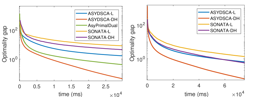
Figure 2: LASSO. Left: undirected graph. We set $\tilde{\mu}=8$ and $\gamma=0.008$ in ASY-DSCA-L; $\tilde{\mu}=1$ and $\gamma=0.008$ in ASY-DSCA-DH; $\alpha=0.06$ and $\eta=0.6$ in AsyPrimalDual; $\tilde{\mu}=1$ and $\gamma=0.002$ in SONATA-L; and $\tilde{\mu}=1$ and $\gamma=0.005$ in SONATA-DH. right: directed graph (each agent is of 10 out-neighbors). We set $\tilde{\mu}=10$ and $\gamma=0.01$ in ASY-DSCA-L; $\tilde{\mu}=10$ and $\gamma=0.03$ in ASY-DSCA-DH; $\tilde{\mu}=10$ and $\gamma=0.03$ in SONATA-L; and $\tilde{\mu}=10$ and $\gamma=0.05$ in SONATA-DH.

The decentralized LASSO problem reads

$$\min_{x\in\mathbb{R}^{n}}U(x)\triangleq\sum_{i\in[I]}\|M_{i}x-b_{i}\|^{2}+\lambda\left\lVert x\right\rVert_{1}.\vspace{-0.2cm}$$ (14)

Data $(M_{i},b_{i})_{i\in[I]}$ are generated as follows. We choose $x_{0}\in\mathbb{R}^{n}$ as a ground truth sparse vector, with $density*n$ nonzero entries drawn i.i.d. from $\mathcal{N}(0,1)$. Each row of $M_{i}\in\mathbb{R}^{r\times n}$ is drawn i.i.d. from $\mathcal{N}(0,\Sigma)$ with $\Sigma$ as a diagonal matrix such that $\Sigma_{i,i}=i^{-\omega}$. We use $\omega$ to control the conditional number of $\Sigma.$ Then we generate $b_{i}=M_{i}x_{0}+\delta_{i}$, with each entry of $\delta_{i}$ drawn i.i.d. from $\mathcal{N}(0,0.01)$. We set $r=10$, $n=300$, $I=20$, $\lambda=2$, $\omega=1.1$ and $density=0.3$. Since the problem satisfies the LT condition, we use $\frac{1}{I}\sum_{i\in[I]}U\left(x_{i}^{k}\right)-U^{\star}$ as the optimality measure. The result are reported in Fig. 2.

5.2 Sparse logistic regression

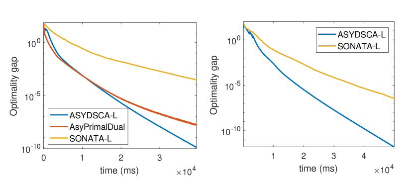
Figure 3: Logistic regression. Left: undirected graph. We set $\tilde{\mu}=10$ and $\gamma=0.06$ in ASY-DSCA-L; $\alpha=0.1$ and $\eta=0.7$ in AsyPrimalDual; and $\tilde{\mu}=10$ and $\gamma=0.08$ in SONATA-L. right: directed graph (each agent is of 10 out-neighbors). We set $\tilde{\mu}=10$ and $\gamma=0.05$ in ASY-DSCA-L; and $\tilde{\mu}=10$ and $\gamma=0.1$ in SONATA-L.

We consider the decentralized sparse logistic regression problem in the following form

$$\min_{x\in\mathbb{R}^{n}}\sum_{i\in[I]}\sum_{s\in\mathcal{D}_{i}}\log(1+\exp(-y_{s}\,u_{s}^{\top}x))+\lambda\left\lVert x\right\rVert_{1},\vspace{-0.2cm}$$

Data $(u_{s},y_{s})$, ${s\in\cup_{i\in[I]}\mathcal{D}_{i}}$, are generated as follows. We first choose $x_{0}\in\mathbb{R}^{n}$ as a ground truth sparse vector with $density*n$ nonzero entries drawn i.i.d. from $\mathcal{N}(0,1)$. We generate each sample feature $u_{s}$ independently, with each entry drawn i.i.d. from $\mathcal{N}(0,1)$; then we set $y_{s}=1$ with probability $1/(1+\exp(-u_{s}^{\top}x_{0}))$, and $y_{s}=-1$ otherwise. We set $\left|\mathcal{D}_{i}\right|=3,\forall i\in[I],\,n=100,\,I=20,\,\lambda=0.01$ and $density=0.3.$ We use the same optimality measure as that for the LASSO problem. The results and the tuning of parameters are reported in Fig. 3.

5.3 M-estimator

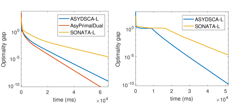
Figure 4: m-estimator. Left: undirected graph. We set $\tilde{\mu}=300$ and $\gamma=0.1$ in ASY-DSCA-L; $\alpha=0.01$ and $\eta=0.6$ in AsyPrimalDual; and $\tilde{\mu}=100$ and $\gamma=0.1$ in SONATA-L. right: directed graph (each agent is of 7 out-neighbors). We set $\tilde{\mu}=1000$ and $\gamma=0.08$ in ASY-DSCA-L; and $\tilde{\mu}=1000$ and $\gamma=0.2$ in SONATA-L.

As nonconvex (constrained, nonsmooth) instance of problem (P), we consider the following M-estimation task [zhang2019robustness, (17)]:

$$\min_{\left\lVert x\right\rVert_{2}\leq r}\frac{1}{\left|\mathcal{D}\right|}\sum_{i\in[I]}\sum_{s\in\mathcal{D}_{i}}\rho_{\alpha}(u_{s}^{\top}x-y_{s})+\lambda\left\lVert x\right\rVert_{1},\vspace{-0.1cm}$$ (15)

where $\rho_{\alpha}(t)=(1-e^{-\alpha\,t^{2}/2})/\alpha$ is the nonconvex Welsch’s exponential squared loss and $\mathcal{D}\triangleq\cup_{i\in[I]}\mathcal{D}_{i}$. We generate $x_{0}\in\mathbb{R}^{n}$ as unit norm sparse vector with $density*n$ nonzero entries drawn i.i.d. from $\mathcal{N}(0,1)$. Each entry of $u_{s}\in\mathbb{R}^{n}$ is drawn i.i.d. from $\mathcal{N}(0,1)$; we generate $y_{s}={u_{s}}^{\top}x_{0}+0.1*\epsilon_{s}$, with $\epsilon_{s}\overset{i.i.d.}{\sim}\mathcal{N}(0,1)$. We set $\left|\mathcal{D}_{i}\right|=10$, for all $i\in[I]$, $n=100$, $I=30,$ $\alpha=0.1,$ $r=2$, $\lambda=0.01$, and $density=0.1.$ Since (15) is nonconvex, progresses towards stationarity and consensus are measured using the merit function $M_{F}(\cdot)$ in (13). The result and tuning of parameters are reported in Fig. 4.

5.4 Discussion

All the experiments clearly show that ASY-DSCA achieves linear rate on LASSO and Logistic regression, with nonstrongly convex objectives, both over undirected and directed graphs–this supports our theoretical findings (Theorem 1). The flexibility in choosing the surrogate functions provides us the chance to better exploit the curvature of the objective function than plain linearization-based choices. For example, in the LASSO experiment, ASY-DSCA-DH outperforms all the other schemes due to its advantage of better exploiting second order information. Also, ASY-DSCA compares favorably with AsyPrimalDual. ASY-DSCA exhibits good performance also in the nonconvex setting (recall that no convergence proof is available for AsyPrimalDual applied to nonconvex problems). In our experiments, asynchronous algorithms turned to be faster than synchronous ones. The reason is that, at each iteration, agents in synchronous algorithms must wait for the slowest agent receiving the information and finishing its computation (no delays are allowed), before proceeding to the next iteration. This is not the case of asynchronous algorithms wherein agents communicate and update continuously with no coordination.

6 Proof of Theorem 1

6.1 Roadmap of the proof

We begin introducing in this section the roadmap of the proof. Define ${x}^{k}\triangleq[{x}_{1}^{k},\cdots,{x}_{I}^{k}]^{\top}$, ${v}^{k}\triangleq[{v}_{1}^{k},\cdots,{v}_{I}^{k}]^{\top}\in\mathbb{R}^{I\times n}$; and let $S\triangleq(D+2)I.$ Construct the two $S\times n$ matrices:

$$\Delta H^{k}\triangleq{e}_{i^{k}}\left(\Delta x^{k}\right)^{\top},\quad\text{with}\quad\Delta x^{k}\triangleq\widetilde{x}_{i^{k}}^{k}-{x}_{i^{k}}^{k},$$

$$H^{k}\triangleq[({x}^{k})^{\top},({v}^{k})^{\top},({v}^{k-1})^{\top},\cdots,({v}^{k-D})^{\top}]^{\top},$$

with ${v}^{t}=0$, for $t\leq 0$. Our proof builds on the following quantities that monitor the progress of the algorithm.

• Optimality gaps:

  $$\Delta^{k}\triangleq\|\widetilde{x}_{i^{k}}^{k}-x_{i^{k}}^{k}\|,\quad E_{{o}}^{k}\triangleq\max_{i\in[S]}U(H_{i}^{k})-U^{\ast};\vspace{-0.1cm}$$ (16a)

• Consensus errors ($x_{\psi}^{k}$ is some weighted average of row vectors of $H^{k}$ and will be defined in Sec. 6.2):

  $$E_{{x}}^{k}\triangleq\left\lVert H^{k}-\bm{1}\cdot x_{\psi}^{k}\right\rVert,\quad E_{{y}}^{k}\triangleq\left\lVert{y}_{i^{k}}^{k}-\bar{g}^{k}\right\rVert;\vspace{-0.1cm}$$ (16b)

• Tracking error:

  $$E_{{t}}^{k}\triangleq\left\lVert Iy_{i^{k}}^{k}-\nabla F(x_{i^{k}}^{k})\right\rVert^{2}.\vspace{-0.1cm}$$ (16c)

Specifically, $\Delta^{k}$ and $E_{{o}}^{k}$ measure the distance of the $x_{i}^{k}$’s from optimality in terms of step-length and objective value. $E_{{x}}^{k}$ and $E_{{y}}^{k}$ represents the consensus error of $x_{i}$’s and $y_{i}$’s, respectively while $E_{{t}}^{k}$ is the tracking error of $y_{i}^{k}$. Our goal is to show that the above quantities vanish at a linear rate, implying convergence (at the same rate) of the iterates generated by the algorithm to a solution of Problem (P). Since each of them affects the dynamics of the others, our proof begins establishing the following set of inequalities linking these quantities (the explicit expression of the constants below will be given in the forthcoming sections):

$$\begin{split}&E_{{y}}^{k+1}\leq 3C_{1}l\sum_{l=0}^{k}\rho^{k-l}\left(E_{{x}}^{l}+\gamma\Delta^{l}\right)+C_{1}\rho^{k}\left\lVert{g}^{0}\right\rVert,\end{split}$$ (17a)

$$\begin{split}&E_{{x}}^{k+1}\leq C_{2}\rho^{k}E_{{x}}^{0}+C_{2}\sum_{l=0}^{k}\rho^{k-l}\gamma\Delta^{l},\end{split}$$ (17b)

$$\begin{split}&E_{{t}}^{k}\leq 8I\,l^{2}(E_{{x}}^{k})^{2}+2I^{2}(E_{{y}}^{k})^{2},\end{split}$$ (17c)

$$\begin{split}&E_{{o}}^{k+1}\leq C_{4}(\gamma)\,\zeta(\gamma)^{k}E_{{o}}^{0}+\frac{C_{3}(\gamma)C_{4}(\gamma)}{\zeta(\gamma)}\sum_{\ell=0}^{k}\zeta(\gamma)^{k-\ell}E_{{t}}^{\ell},\end{split}$$ (17d)

$$\begin{split}&(\Delta^{k})^{2}\leq\frac{1}{\gamma\left(\tilde{\mu}-\frac{\epsilon}{2}-\frac{\gamma L}{2}\right)}E_{{o}}^{k}+\frac{1}{2\,\epsilon\left(\tilde{\mu}-\frac{\epsilon}{2}-\frac{\gamma L}{2}\right)}E_{{t}}^{k}.\end{split}$$ (17e)

We then show that $\Delta^{k}$, $E_{{o}}^{k}$, $E_{{x}}^{k}$, $E_{{y}}^{k}$ and $E_{{y}}^{k}$ vanish at linear rate chaining the above inequalities by means of the generalized small gain theorem [Tian_arxiv].

The main steps of the proof are summarized next.

$\bullet$ Step 1: Proof of (17a)-(17c) via P-ASY-SUM-PUSH. We rewrite (S.2) and (S.3) in ASY-DSCA (Algorithm 2) as instances of the perturbed asynchronous consensus scheme and the perturbed asynchronous sum-push scheme (the P-ASY-SUM-PUSH) introduced in the companion paper [Tian_arxiv]. By doing so, we can bound the consensus errors $E_{{x}}^{k}$ and $E_{{y}}^{k}$ in terms of $\Delta^{k}$ and then prove (17a)-(17b)–see Lemma 4 and Lemma 5. Eq. (17c) follows readily from (17a)-(17b)–see Lemma 6.

$\bullet$ Step 2: Proof of (17d)-(17e) under the LT condition. Proving (17d)–contraction of the optimality measure $E_{{o}}^{k}$ up to the tracking error–poses several challenges. To prove contraction of some form of optimization errors, existing techniques developed in the literature of distributed algorithms [shi2015extra, Nedich-geometric, qu2017harnessing, sun2019convergence, alghunaim2019decentralized] (including our companion paper [Tian_arxiv]) leverage strong convexity of $F$, a property that is replaced here by the weaker local growing condition (2) in the LT error bound. Hence, they are not applicable to our setting. On the other hand, existing proofs showing linear rate of centralized first-order methods under the LT condition [luo1993error] do not readily customize to our distributed, asynchronous setting, for the reasons elaborated next. To invoke the local growing condition (2), one needs first to show that the sequences generated by the algorithm enters (and stays into) the region where (1) holds, namely: a) the function value remains bounded; and b) the proximal operator residual is sufficiently small. A standard path to prove a) and b) in the centralized setting is showing that the objective function sufficiently descents along the trajectory of the algorithm. Asynchrony apart, in the distributed setting, function values on the agents’ iterates do not monotonically decrease provably, due to consensus and gradient tracking errors. To cope with these issues, in this Step 2, we put forth a new analysis. Specifically, i) Sec. 6.3.1: we build a novel Lyapunov function [cf. (28)] that linearly combines objective values of current and past (up to $D$) iterates (all the elements of $H^{k}$); notice that the choice of the weights (cf. ${\psi}^{k}$ in Lemma 3) is very peculiar and represents a major departure from existing approaches (including our companion paper [Tian_arxiv])–${\psi}^{k}$ endogenously vary according to the asynchrony trajectory of the algorithm. The Lyapunov function is proved to “sufficiently” descent over the asynchronous iterates of ASY-DSCA (cf. Proposition 8); ii) Sec. 6.3.2: building on such descent properties, we manage to prove that $x_{i^{k}}^{k}$ will eventually satisfy the aforementioned conditions (1) (cf. Lemma 10 & Corollary 9), so that the LT growing property (2) can be invoked at $x_{i^{k}}^{k}$ (cf. Corollary 11); iii) Sec. 6.3.4: Finally, leveraging this local growth, we uncover relations between $E_{{o}}^{k}$ and $E_{{t}}^{k}$ and prove (17d) (cf. Proposition 12). Eq. (17e) is proved in Sec. 6.3.4 by product of the derivations above.

$\bullet$ Step 3: R-linear convergence via the generalized small gain theorem. We complete the proof of linear convergence by applying [Tian_arxiv, Th. 23] to the inequality system (17), and conclude that all the local variables $\{x_{i}\}_{i\in[I]}$ converge to the set of optimal solutions $\mathcal{K}^{\ast}$ R-linearly.

6.2 Step 1: Proof of (17a)-(17c)

We interpret the consensus step (S.2) in Algorithm 2 as an instance of the perturbed asynchronous consensus scheme [Tian_arxiv]: (8) can be rewritten as

$${H}^{k+1}=\widehat{{W}}^{k}({H}^{k}+\gamma\Delta H^{k}),$$ (18)

where $\widehat{{W}}^{k}$ is a time-varying augmented matrix induced by the update order of the agents and the delay profile. The specific expression of $\widehat{{W}}^{k}$ can be found in [Tian_arxiv] and is omitted here, as it is not relevant to the convergence proof. We only need to recall the following properties of $\widehat{{W}}^{k}$.

Lemma 3.

[Tian_arxiv, Lemma 17] Let $\{\widehat{{W}}^{k}\}_{k\in\mathbb{N}_{+}}$ be the sequence of matrices in the dynamical system (18), generated under Assumption 6, and with ${W}$ satisfying Assumption 5 (i), (ii). Define $K_{1}\triangleq(2I-1)\cdot T+I\cdot D$, $C_{2}\triangleq\frac{2\sqrt{(D+2)I}(1+\bar{m}^{-K_{1}})}{1-\bar{m}^{-K_{1}}}$, $\eta\triangleq\bar{m}^{K_{1}}$ and $\rho\triangleq(1-\eta)^{\frac{1}{K_{1}}}$. Then we have for any $k\geq 0$:

1. $\widehat{{W}}^{k}$ is row stochastic;

2. all the entries in the first $I$ columns of $\widehat{{W}}^{k+K_{1}-1:k}$ are uniformly bounded below by $\eta;$

3. there exists a sequence of stochastic vectors $\{{\psi}^{k}\}_{k\geq 0}$ such that: i) for any $\ell\geq t\geq 0$, $\left\lVert\widehat{{W}}^{\ell:t}-\mathbf{1}{{\psi}^{t}}^{\top}\right\rVert_{2}\leq C_{2}\rho^{\ell-t}$; ii) $\psi_{i}^{k}\geq\eta\,$ for all $i\in\mathcal{V}$.

Note that Lemma 3 implies

$$\mathbf{1}{{\psi}^{t}}^{\top}=\lim_{n\to\infty}\widehat{{W}}^{n:t}=(\lim_{n\to\infty}\widehat{{W}}^{n:t+1})\widehat{{W}}^{t}=\mathbf{1}{{\psi}^{t+1}}^{\top}\widehat{{W}}^{t},$$ (19)

and thus ${{\psi}^{t+1}}^{\top}\widehat{{W}}^{t}={{\psi}^{t}}^{\top}$, for all $t\geq 0.$ Then we define

$$\vspace{-0.2cm}x_{\psi}^{k}={{\psi}^{k}}^{\top}{H}^{k};$$ (20)

$x_{\psi}^{k}$ evolves according to the following dynamics:

$$x_{\psi}^{k+1}={\mathbf{{\psi}}^{0}}^{\top}{H}^{0}+\sum_{l=0}^{k}\gamma{\mathbf{{\psi}}^{l}}^{\top}\Delta{H}^{l}.\vspace{-0.2cm}$$ (21)

This can be shown by applying (18) recursively, so that

$$\vspace{-0.2cm}{H}^{k+1}=\widehat{{W}}^{n:0}{H}^{0}+\sum_{l=0}^{k}\widehat{{W}}^{n:l}\gamma\Delta{H}^{l},$$ (22)

and multiplying (22) from the left by ${{\psi}^{k+1}}^{\top}$ and using (19). Taking the difference between (21) and (22) and applying Lemma 3 the consensus error $E_{{x}}^{k}$ can be bound as follows.

Lemma 4.

Under the condition of Lemma 3, $\{E_{{x}}^{k}\}$ satisfies

$$E_{{x}}^{k+1}\leq C_{2}\,\rho^{k}\,E_{{x}}^{0}+C_{2}\sum_{l=0}^{k}\rho^{k-l}\gamma\,\Delta^{l},\quad\forall k\geq 0.\vspace{-0.2cm}$$ (23)

To establish similar bounds for $E_{y}^{k}$, we build on the fact that the gradient tracking update (9) is an instance of the P-ASY-SUM-PUSH in [Tian_arxiv], as shown next. Define

$$g^{k}=[\nabla f_{1}(x_{1}^{k}),\nabla f_{2}(x_{2}^{k}),\cdots,\nabla f_{I}(x_{I}^{k})]^{\top},$$

$$\bar{g}^{k}=(1/I)\cdot(g^{k})^{\top}\mathbf{1},\qquad E_{{y}}^{k}\triangleq\left\lVert{y}_{i^{k}}^{k}-\bar{g}^{k}\right\rVert.$$

We can prove the following bound for $E_{{y}}^{k}$.

Lemma 5.

Let $\{x^{k},y_{i^{k}}^{k}\}_{k=0}^{\infty}$ be the sequence generated by the Algorithm 2 under Assumption 2, 5, and 6. Then, there exists a constant $C_{1}=\frac{4\sqrt{2S}(1+\bar{m}^{-K_{1}})}{I\,\eta\,\rho(1-\bar{m}^{K_{1}})}$ such that

$$E_{{y}}^{k+1}\leq 3\,C_{1}\,l\sum_{l=0}^{k}\rho^{k-l}\left(E_{{x}}^{l}+\gamma\Delta^{l}\right)+C_{1}\rho^{k}\left\lVert{g}^{0}\right\rVert.\vspace{-0.1cm}$$ (24)

Proof.

See Appendix A.∎

Finally, using Lemma 4 and Lemma 5, we can bound $\sum_{t=0}^{k}(E_{{x}}^{t})^{2}$ and $\sum_{t=0}^{k}(E_{{y}}^{t})^{2}$ in terms of $\sum_{t=0}^{k}\gamma^{2}(\Delta^{t})^{2}$, and $E_{{t}}^{k}$ in terms of $E_{{x}}^{k}$ and $E_{{y}}^{k}$, as given below.

Lemma 6.

Under the setting of Lemma 4 and Lemma 5, we have: for any $k\geq 1$,

$$\sum_{t=0}^{k}(E_{{x}}^{t})^{2}\leq c_{x}+\varrho_{x}\sum_{t=0}^{k}\gamma^{2}(\Delta^{t})^{2},$$

$$\sum_{t=0}^{k}(E_{{y}}^{t})^{2}\leq c_{y}+\varrho_{y}\sum_{t=0}^{k}\gamma^{2}(\Delta^{t})^{2},$$

$$E_{{t}}^{k}\leq 2I^{2}(E_{{y}}^{k})^{2}+8I\,l^{2}\,(E_{{x}}^{k})^{2}.$$ (25)

with $\varrho_{x}\triangleq\frac{2C_{2}^{2}}{(1-\rho)^{2}},$ and $\varrho_{y}\triangleq\frac{36\left(C_{1}L\right)^{2}\left(2C_{2}^{2}+(1-\rho)^{2}\right)}{(1-\rho)^{4}}.$ (The expressions of the constants $c_{x}$ and $c_{y}$ are omitted as they are not relevant).

Proof.

The proof of the first two results follows similar steps as in that of [Tian_arxiv, Lemma 26] and thus is omitted. We prove only the last inequality, as follows:

$$E_{{t}}^{k}=\left\lVert Iy_{i^{k}}^{k}\pm I\bar{g}^{k}-\nabla F(x_{i^{k}}^{k})\right\rVert^{2}$$

$$\leq 2I^{2}(E_{{y}}^{k})^{2}+2\Big{\|}\sum_{j=1}^{I}f_{j}(x_{j}^{k})\pm F(x_{\psi}^{k})-\nabla F(x_{i^{k}}^{k})\Big{\|}^{2}$$

$$\leq 2I^{2}(E_{{y}}^{k})^{2}+8I\,l^{2}\,(E_{{x}}^{k})^{2}.$$

∎

6.3 Step 2: Proof of (17d)-(17e) under the LT condition

6.3.1 A new Lyapunov function and its descent

We begin studying descent of the objective function $U$ along the trajectory of the algorithm; we have the following result.

Lemma 7.

Let $\{(x^{k},y^{k})\}$ be the sequence generated by Algorithm 2 under Assumptions 1 and 4, it holds

$$U(v_{i^{k}}^{k+1})\leq \,U(x_{i^{k}}^{k})-\gamma\left(\tilde{\mu}-\frac{\gamma L}{2}\right)\left\lVert\Delta x^{k}\right\rVert^{2}$$

$$+\gamma\cdot\left(\nabla F(x_{i^{k}}^{k})-Iy_{i^{k}}^{k}\right)^{\top}\Delta x^{k}.$$ (26)

Proof.

Applying the first order optimality condition to (7) and invoking the strong convexity of $\widetilde{f}_{i^{k}}$ (Assumption 4) we have

$$-(\Delta x^{k})^{\top}Iy_{i^{k}}^{k}+G(x_{i^{k}}^{k})-G(\widetilde{x}_{i^{k}}^{k})$$ (27)

$$\geq-(\Delta x^{k})^{\top}(\nabla f_{i^{k}}(x_{i^{k}}^{k})-\nabla\widetilde{f}_{i^{k}}(\widetilde{x}_{i^{k}}^{k};x_{i^{k}}^{k}))$$

$$=(\Delta x^{k})^{\top}\big{(}\nabla\widetilde{f}_{i^{k}}(\widetilde{x}_{i^{k}}^{k};x_{i^{k}}^{k})-\nabla\widetilde{f}_{i^{k}}(x_{i^{k}}^{k};x_{i^{k}}^{k})\big{)}\geq\tilde{\mu}\cdot\left\lVert\Delta x^{k}\right\rVert^{2}.$$

As $F$ is $L$-smooth, applying the descent lemma gives

$$\begin{split}&F(v_{i^{k}}^{k+1})\leq F(x_{i^{k}}^{k})+\gamma\cdot\nabla F(x_{i^{k}}^{k})^{\top}\Delta x^{k}+\frac{L}{2}\gamma^{2}\left\lVert\Delta x^{k}\right\rVert^{2}\\ &=F(x_{i^{k}}^{k})+\gamma\cdot(Iy_{i^{k}}^{k})^{\top}\Delta x^{k}+\gamma\cdot\left(\nabla F(x_{i^{k}}^{k})-Iy_{i^{k}}^{k}\right)^{\top}\Delta x^{k}+\frac{L}{2}\gamma^{2}\left\lVert\Delta x^{k}\right\rVert^{2}\\ &\overset{\eqref{eq:mini_prin}}{\leq}F(x_{i^{k}}^{k})+\gamma\left(G(x_{i^{k}}^{k})-G(\widetilde{x}_{i^{k}}^{k})-\tilde{\mu}\left\lVert\Delta x^{k}\right\rVert^{2}\right)+\frac{L}{2}\gamma^{2}\left\lVert\Delta x^{k}\right\rVert^{2}+\gamma\cdot\left(\nabla F(x_{i^{k}}^{k})-Iy_{i^{k}}^{k}\right)^{\top}\Delta x^{k}.\end{split}$$

By the convexity of $G$, we have

$$\gamma\left(G(x_{i^{k}}^{k})-G(\widetilde{x}_{i^{k}}^{k})\right)\leq G(x_{i^{k}}^{k})-G(v_{i^{k}}^{k+1}).$$

Combining the above two results proves (7). ∎

We build now on (7) and establish descent on a suitable defined Lyapunov function. Define the mapping $\widetilde{U}:\mathbb{R}^{S\times n}\to\mathbb{R}^{S}$ as $\widetilde{U}(H)=[U(h_{1}),\cdots,U(h_{S})]^{\top}$ for $H=[h_{1},\cdots,h_{S}]^{\top}\in\mathbb{R}^{S\times n}$. That is, $\widetilde{U}(H)$ is a vector constructed by stacking the value of the objective function $U$ evaluated at each local variable $h_{i}$. Recalling the definition of the weights ${\psi}^{k}$ (cf. Lemma 3), we introduce the Lyapunov function

$${L}^{k}\triangleq{{\psi}^{k}}^{\top}\widetilde{U}(H^{k}),\vspace{-0.2cm}$$ (28)

and study next its descent properties.

Proposition 8.

Let $\{(x^{k},v^{k},y^{k})\}$ be the sequence generated by Algorithm 2 under Assumptions 1, 2, 4, and 5. Then,

$${L}^{k+1}\leq{L}^{0}$$ (29)

$$\leavevmode\nobreak\ -\sum_{t=0}^{k}(\Delta^{t})^{2}\gamma\left(\eta\tilde{\mu}-\gamma\left(\frac{L}{2}+l\,I^{\frac{3}{2}}\sqrt{\varrho_{x}}+I\sqrt{\varrho_{y}}\right)\right)+C,$$

for all $k\geq 0$, where $C$ is some constant independent of $\gamma$ and $k$; and $\varrho_{x}$ and $\varrho_{y}$ are defined in Lemma 6.

Proof.

By the row stochasticity of $\widehat{{W}}$ and the convexity of $U$:

$$\widetilde{U}(H^{k+1})=\widetilde{U}\left(\widehat{{W}}^{k}(H^{k}+\gamma\Delta{H}^{k})\right)\preccurlyeq\widehat{{W}}^{k}\,\widetilde{U}\left(H^{k}+\gamma\Delta{H}^{k}\right)$$

$$\preccurlyeq\widehat{{W}}^{k}\bigg{(}\widetilde{U}(H^{k})-\bigg{(}\gamma\bigg{(}\tilde{\mu}-\frac{\gamma L}{2}\bigg{)}\left\lVert\Delta x^{k}\right\rVert^{2}-\gamma\cdot\big{(}\nabla F(x_{i^{k}}^{k})-Iy_{i^{k}}^{k}\big{)}^{\top}\Delta x^{k}\bigg{)}{e}_{i^{k}}\bigg{)},$$

where in the last inequality we applied Lemma 7. Using now Lemma 3, we have

$$\begin{split}&{L}^{k+1}\\ &\leq{L}^{k}-\psi_{i^{k}}^{k}\bigg{(}\gamma\bigg{(}\tilde{\mu}-\frac{\gamma L}{2}\bigg{)}\left\lVert\Delta x^{k}\right\rVert^{2}\!\!\!-\gamma\left(\nabla F(x_{i^{k}}^{k})-Iy_{i^{k}}^{k}\right)^{\top}\!\!\!\Delta x^{k}\bigg{)}\\ &\leq{L}^{k}-\gamma\eta\tilde{\mu}\left\lVert\Delta x^{k}\right\rVert^{2}+\frac{L(\gamma)^{2}}{2}\left\lVert\Delta x^{k}\right\rVert^{2}+\psi_{i^{k}}^{k}\,\gamma\left(\nabla F(x_{i^{k}}^{k})-Iy_{i^{k}}^{k}\right)^{\top}\Delta x^{k}\\ &\leq{L}^{k}-\gamma\left(\eta\tilde{\mu}-\frac{\gamma L}{2}\right)\left\lVert\Delta x^{k}\right\rVert^{2}\\ &\quad+\psi_{i^{k}}^{k}\gamma\left(\nabla F(x_{i^{k}}^{k})\pm I\bar{g}^{k}-I\,y_{i^{k}}^{k}\right)^{\top}\Delta x^{k}\\ &\leq{L}^{k}-\gamma\left(\eta\tilde{\mu}-\frac{\gamma L}{2}\right)\left\lVert\Delta x^{k}\right\rVert^{2}+\gamma\,I\,l\sum_{j=1}^{I}\left\lVert x_{\psi}^{k}-x_{j}^{k}\right\rVert\left\lVert\Delta x^{k}\right\rVert+\gamma\,IE_{{y}}^{k}\,\cdot\left\lVert\Delta x^{k}\right\rVert\\ &\leq{L}^{k}-\gamma\left(\eta\tilde{\mu}-\frac{\gamma L}{2}\right)\left\lVert\Delta x^{k}\right\rVert^{2}+\gamma\,l\,I^{\frac{3}{2}}E_{{x}}^{k}\,\left\lVert\Delta x^{k}\right\rVert+\gamma\,IE_{{y}}^{k}\,\cdot\left\lVert\Delta x^{k}\right\rVert^{2}\\ &\overset{(*)}{\leq}{L}^{k}-\gamma\left(\eta\tilde{\mu}-\gamma\left(\frac{L}{2}+\frac{1}{2\epsilon_{1}}+\frac{1}{2\epsilon_{2}}\right)\right)\left\lVert\Delta x^{k}\right\rVert^{2}+\frac{\epsilon_{1}}{2}\,l^{2}\,I^{3}(E_{{x}}^{k})^{2}+\frac{\epsilon_{2}}{2}\,I^{2}(E_{{y}}^{k})^{2}\\ &\leq{L}^{0}-\gamma\left(\eta\tilde{\mu}-\gamma\left(\frac{L}{2}+\frac{1}{2\epsilon_{1}}+\frac{1}{2\epsilon_{2}}\right)\right)\sum_{t=0}^{k}\left\lVert\Delta x^{t}\right\rVert^{2}+\frac{\epsilon_{1}}{2}\,l^{2}\,I^{3}\sum_{t=0}^{k}(E_{{x}}^{t})^{2}+\frac{\epsilon_{2}}{2}\,I^{2}\sum_{t=0}^{k}(E_{{y}}^{t})^{2},\end{split}$$

where ($*$) follows from the Young’s inequality with $\epsilon_{1,2}>0$. Invoking Lemma 6 and setting $\gamma^{l}\equiv\gamma$ gives (29), where the free parameters $\epsilon_{1,2}$ are chosen as $\epsilon_{1}={1}/({l\,I^{\frac{3}{2}}\sqrt{\varrho_{x}}})$ and $\epsilon_{2}={1}/({I\sqrt{\varrho_{y}}})$, respectively. ∎

6.3.2 Leveraging the LT condition

We build now on Proposition 8 and show next that the two conditions in (1) holds at $x_{i}^{k}$, for sufficiently large $k$; this will permit to invoke the LT growing property (2).

The first condition–$U(x_{i}^{k})$ bounded for large $k$–is a direct consequence of Proposition 8 and the facts that $U$ is bounded from below (Assumption 1) and $\psi_{i}^{k}\geq\eta$, for all $i\in[I]$ and $k\geq 0$. Formally, we have the following.

Corollary 9.

Under the setting of Proposition 8 and step-size $0<\gamma<\bar{\gamma}\triangleq\frac{2\eta\tilde{\mu}}{L+2l\,I^{\frac{3}{2}}\sqrt{\varrho_{x}}+2I\sqrt{\varrho_{y}}}$, it holds:

1. $U(x_{i}^{k})$ is uniformly upper bounded, for all $i\in\mathcal{V}$ and $k\geq 0$;

2. $\sum_{t=0}^{\infty}(\Delta^{t})^{2}<\infty$, $\sum_{t=0}^{\infty}(E_{{x}}^{t})^{2}<\infty$, and $\sum_{t=0}^{\infty}(E_{{y}}^{t})^{2}<\infty$.

We prove now that the second condition in (1) holds for large $k$–the residual of the proximal operator at $x_{i^{k}}^{k}$, that is $\left\lVert x_{i^{k}}^{k}-\text{prox}_{G}(x_{i^{k}}^{k}-\nabla F(x_{i^{k}}^{k}))\right\rVert$, is sufficiently small. Since $\Delta^{k}$ and the gradient tracking error $E_{{t}}^{k}$ are vanishing [as a consequence of Corollary 9ii) and Lemma 6], it is sufficient to bound the aforementioned residual by $\Delta^{k}$ and $E_{{t}}^{k}$. This is done in the lemma below.

Lemma 10.

The proximal operator residual on $x_{i^{k}}^{k}$ satisfies $\left\lVert x_{i^{k}}^{k}-\text{prox}_{G}(x_{i^{k}}^{k}-\nabla F(x_{i^{k}}^{k}))\right\rVert^{2}\leq 4\big{(}1+(l+\tilde{l})^{2}\big{)}(\Delta^{k})^{2}+5E_{{t}}^{k}.$

Proof.

For simplicity, we denote $\hat{x}^{k}=\text{prox}_{G}(x_{i^{k}}^{k}-\nabla F(x_{i^{k}}^{k}))$. According to the variational characterization of the proximal operator, we have, for all $w\in\mathcal{K}$,

$$\left(\hat{x}^{k}-\big{(}x_{i^{k}}^{k}-\nabla F(x_{i^{k}}^{k})\big{)}\right)^{\top}(\hat{x}^{k}-w)+G(\hat{x}^{k})-G(w)\leq 0.$$

The first order optimality condition of $\widetilde{x}_{i^{k}}^{k}$ implies

$$\left(\nabla\widetilde{f}_{i^{k}}(\widetilde{x}_{i^{k}}^{k};x_{i^{k}}^{k})+Iy_{i^{k}}^{k}-\nabla f_{i^{k}}(x_{i^{k}}^{k})\right)^{\top}(\widetilde{x}_{i^{k}}^{k}-z)+G(\widetilde{x}_{i^{k}}^{k})-G(z)\leq 0,\quad\forall z\in\mathcal{K}.$$ (30)

Setting $z=\hat{x}^{k}$ and $w=\widetilde{x}_{i^{k}}^{k}$ and adding the above two inequalities yields

$$0\geq\bigg{(}\nabla\widetilde{f}_{i^{k}}(\widetilde{x}_{i^{k}}^{k};x_{i^{k}}^{k})+Iy_{i^{k}}^{k}-\nabla f_{i^{k}}(x_{i^{k}}^{k})-\hat{x}^{k}+x_{i^{k}}^{k}-\nabla F(x_{i^{k}}^{k})\bigg{)}^{\top}(\widetilde{x}_{i^{k}}^{k}-\hat{x}^{k})$$

$$=\left(Iy_{i^{k}}^{k}-\hat{x}^{k}+x_{i^{k}}^{k}-\nabla F(x_{i^{k}}^{k})\right)^{\top}(\widetilde{x}_{i^{k}}^{k}-x_{i^{k}}^{k})+\left(\nabla\widetilde{f}_{i^{k}}(\widetilde{x}_{i^{k}}^{k};x_{i^{k}}^{k})-\nabla f_{i^{k}}(x_{i^{k}}^{k})\right)^{\top}(\widetilde{x}_{i^{k}}^{k}-x_{i^{k}}^{k})$$

$$\leavevmode\nobreak\ \leavevmode\nobreak\ +\left\lVert\hat{x}^{k}-x_{i^{k}}^{k}\right\rVert^{2}+\bigg{(}\nabla\widetilde{f}_{i^{k}}(\widetilde{x}_{i^{k}}^{k};x_{i^{k}}^{k})+Iy_{i^{k}}^{k}-\nabla f_{i^{k}}(x_{i^{k}}^{k})-\nabla F(x_{i^{k}}^{k})\bigg{)}^{\top}(x_{i^{k}}^{k}-\hat{x}^{k})$$

$$\geq-\frac{1}{2}\left\lVert Iy_{i^{k}}^{k}-\nabla F(x_{i^{k}}^{k})\right\rVert^{2}-\frac{1}{2}\left\lVert\Delta x^{k}\right\rVert^{2}-\frac{1}{4}\left\lVert\hat{x}^{k}-x_{i^{k}}^{k}\right\rVert^{2}$$

$$\leavevmode\nobreak\ \leavevmode\nobreak\ -\left\lVert\Delta x^{k}\right\rVert^{2}+\widetilde{\mu}\left\lVert\Delta x^{k}\right\rVert^{2}+\left\lVert\hat{x}^{k}-x_{i^{k}}^{k}\right\rVert^{2}-\frac{1}{4}\left\lVert\hat{x}^{k}-x_{i^{k}}^{k}\right\rVert^{2}$$

$$\leavevmode\nobreak\ \leavevmode\nobreak\ -2\left((l+\widetilde{l})^{2}\left\lVert\Delta x^{k}\right\rVert^{2}+\left\lVert Iy_{i^{k}}^{k}-\nabla F(x_{i^{k}}^{k})\right\rVert^{2}\right).$$

Rearranging terms proves the desired result. ∎

Corollary 9 in conjunction with Lemma 10 and Lemma 6 show that both conditions in (1) hold at $\{x^{k}\}$, for large $k$. We can then invoke the growing condition (2).

Corollary 11.

Let $\{x^{k}\}$ be the sequence generated by Algorithm 2 under the setting of Corollary 9. Then, there exists a constant $\kappa>0$ and a sufficiently large $\bar{k}$ such that, for $k\geq\bar{k}$,

$$\text{dist}(x_{i^{k}}^{k},\mathcal{K}^{*})\leq\kappa\,\left\lVert x_{i^{k}}^{k}-\text{prox}_{G}(x_{i^{k}}^{k}-\nabla F(x_{i^{k}}^{k}))\right\rVert.$$ (31)

Proof.

It is sufficient to show that (1) holds at $x_{i^{k}}^{k}$. By Corollary 9(i), $U(x_{i^{k}}^{k})\leq B$, for all $k\geq 0$ and some $B<+\infty$. Lemma 10 in conjunction with Corollary 9(ii) and Lemma 6 yields $\lim\limits_{k\to\infty}\left\lVert x_{i^{k}}^{k}-\text{prox}_{G}(x_{i^{k}}^{k}-\nabla F(x_{i^{k}}^{k}))\right\rVert=0$. ∎

6.3.3 Proof of (17d)

Define

$$C_{3}(\gamma)\triangleq\frac{\gamma\left(c_{6}(\tilde{\mu}-\frac{\epsilon}{2}-\frac{\gamma L}{2})+\frac{c_{7}}{2\epsilon}\right)}{c_{7}+\tilde{\mu}-\frac{\epsilon}{2}-\frac{\gamma L}{2}},$$ (32)

$$C_{4}(\gamma)\triangleq\left(1-\Big{(}1-\sigma(\gamma)\Big{)}\eta\right)^{-1},$$ (33)

$$\zeta(\gamma)\triangleq\left(1-\Big{(}1-\sigma(\gamma)\Big{)}\eta\right)^{\frac{1}{K_{1}}},$$ (34)

$$\sigma(\gamma)\triangleq\frac{c_{7}+\left(\tilde{\mu}-\frac{\epsilon}{2}-\frac{\gamma L}{2}\right)(1-\gamma)}{c_{7}+\tilde{\mu}-\frac{\epsilon}{2}-\frac{\gamma L}{2}},$$ (35)

where $K_{1}=(2I-1)\cdot T+I\cdot D$, and $c_{6},\,c_{7}$ are polynomials in $(1,l,\tilde{l},L,\kappa)$ whose expressions are given in (LABEL:eq:const_expression) and (42); and $\epsilon\in(0,2\tilde{\mu})$ is a free parameter (to be chosen).

In this section, we prove (17d), which is formally stated in the proposition below.

Proposition 12.

Let $\{(x^{k},y^{k})\}$ be the sequence generated by Algorithm 2 under Assumptions 1, 2, 3, 4, and 5. Then, for $k\geq\bar{k}$, it holds

$$E_{{o}}^{k+1}\leq C_{4}(\gamma)\,\zeta(\gamma)^{k}E_{{o}}^{0}+\frac{C_{3}(\gamma)C_{4}(\gamma)}{\zeta(\gamma)}\sum_{\ell=0}^{k}\zeta(\gamma)^{k-\ell}E_{{t}}^{\ell}.\vspace{-0.1cm}$$ (36)

Since $\sigma(\gamma)<1$ for $0<\gamma<\sup_{\epsilon\in(0,2\tilde{\mu})}\frac{2\tilde{\mu}-\epsilon}{L}=\frac{2\tilde{\mu}}{L}$ and $\eta\in(0,1]$, Proposition 12 shows that, for sufficiently small $\gamma>0$, the optimality gap $E_{{o}}^{k}$ converges to zero R-linearly if $E_{{t}}^{k}$ does so. The proof of Proposition 12 follows from Proposition 13 and Lemma 15 below.

Proposition 13.

Let $\{(x^{k},y^{k})\}$ be the sequence generated by Algorithm 2 in the setting of Proposition 12. Let $p^{k}\triangleq\widetilde{U}(H^{k})-U(x^{*})\mathbf{1}$; let ${\Sigma}^{k}$ be the diagonal matrix with all diagonal entries $1$ and ${\Sigma}_{i^{k}i^{k}}^{k}=\sigma(\gamma)$; and let $(\widehat{{W}}{\Sigma})^{k:\ell}\triangleq\widehat{{W}}^{k}{\Sigma}^{k}\cdots\widehat{{W}}^{\ell}{\Sigma}^{\ell}$. Then, for $k\geq\bar{k}$,

$${p}^{k+1}\preccurlyeq\left(\widehat{{W}}{\Sigma}\right)^{k:0}{p}^{0}+C_{3}(\gamma)\sum_{\ell=1}^{k}\left(\widehat{{W}}{\Sigma}\right)^{k:\ell}\widehat{{W}}^{\ell-1}{e}_{i^{\ell-1}}E_{{t}}^{\ell-1}+C_{3}(\gamma)\widehat{{W}}^{k}{e}_{i^{k}}E_{{t}}^{k},$$ (37)

where $C_{3}(\gamma)$ is defined in (32).

Proof.

By convexity of $U$ and (18), we have

$${p}^{k+1} =\widetilde{U}(H^{k+1})-U(x^{*})\mathbf{1}\preccurlyeq\widehat{{W}}^{k}\,\left(\widetilde{U}\left(H^{k}+\gamma\Delta{H}^{k}\right)-U(x^{*})\mathbf{1}\right).$$ (38)

Since $\widetilde{U}\left(H^{k}+\gamma\Delta{H}^{k}\right)$ differs from $\widetilde{U}\left(H^{k}\right)$ only by its $i^{k}$-th row, we study descent occurred at this row, which is $(v_{i^{k}}^{k+1})^{\top}=(x_{i^{k}}^{k}+\gamma\left(\widetilde{x}_{i^{k}}^{k}-x_{i^{k}}^{k}\right))^{\top}.$ Recall that by applying the descent lemma on $F$ and using the convexity of $G$ we proved

$$U(v_{i^{k}}^{k+1})-U(x_{i^{k}}^{k})\leq\frac{L}{2}\gamma^{2}\left\lVert\Delta x^{k}\right\rVert^{2}$$ (39)

$$\leavevmode\nobreak\ \leavevmode\nobreak\ +\gamma\underbrace{\left(\nabla F(x_{i^{k}}^{k})^{\top}\left(\widetilde{x}_{i^{k}}^{k}-x_{i^{k}}^{k}\right)+G(\widetilde{x}_{i^{k}}^{k})-G(x_{i^{k}}^{k})\right)}_{T_{1}}.$$

The above inequality establishes a connections between $U(v_{i^{k}}^{k+1})$ and $U(x_{i^{k}}^{k})$. However, it is not clear whether there is any contraction (up to some error) going from the optimality gap $U(v_{i^{k}}^{k+1})-U^{*}$ to $U(x_{i^{k}}^{k})-U^{*}$. To investigate it, we derive in the lemma below two upper bounds of $T_{1}$ in (39), in terms of $U(v_{i^{k}}^{k+1})-U(x^{*})$ and $\left\lVert\Delta x^{k}\right\rVert$ (up to the tracking error). Building on these bounds and (39) we can finally prove the desired contraction, as stated in (43).

Lemma 14.

$T_{1}$ in (39) can be bounded in the following two alternative ways: for $k\geq\bar{k}$,

$$T_{1}\leq \left(-\tilde{\mu}+\frac{\epsilon}{2}\right)\cdot\left\lVert\Delta x^{k}\right\rVert^{2}+\frac{1}{2\epsilon}\,E_{{t}}^{k},$$ (40)

$$T_{1}\leq -\frac{1}{1-\gamma}\left(U(v_{i^{k}}^{k+1})-U(x^{*})\right)+\frac{1}{1-\gamma}\left(c_{5}\left\lVert\Delta x^{k}\right\rVert^{2}+c_{6}E_{{t}}^{k}\right),$$ (41)

where $c_{5}$ and $c_{6}$ are polynomials in $(1,l,\tilde{l},L,\kappa)$ whose expressions are given in (LABEL:eq:const_expression).

Proof.

See Appendix LABEL:ap:lem:bound_T. ∎

Using Lemma 14 in (39) yields

$$\begin{split}&U(v_{i^{k}}^{k+1})-U^{*}\leq{}(1-\gamma)\left(U(x_{i^{k}}^{k})-U^{*})\right)+\left(\frac{L}{2}\gamma(1-\gamma)+c_{5}\right)\gamma\left\lVert\Delta x^{k}\right\rVert^{2}+c_{6}\cdot\gamma E_{{t}}^{k}\\ &\leq{}(1-\gamma)\left(U(x_{i^{k}}^{k})-U(x^{*}(x_{i^{k}}^{k}))\right)+\underbrace{\left(c_{5}+L/8\right)}_{c_{7}}\gamma\left\lVert\Delta x^{k}\right\rVert^{2}+c_{6}\cdot\gamma E_{{t}}^{k},\end{split}$$ (42a)

and

$$\begin{split}&U(v_{i^{k}}^{k+1})-U^{*}\leq U(x_{i^{k}}^{k})-U^{*}-\left(\tilde{\mu}-\frac{\gamma L}{2}-\frac{\epsilon}{2}\right)\gamma\left\lVert\Delta x^{k}\right\rVert^{2}+\frac{\gamma}{2\epsilon}E_{{t}}^{k}.\end{split}$$ (42b)

Canceling out $\left\lVert\Delta x^{k}\right\rVert^{2}$ in (42a)-(42b) yields: for $k\geq\bar{k}$,

$$U(v_{i^{k}}^{k+1})-U(x^{*})\leq\sigma(\gamma)\left(U(x_{i^{k}}^{k})-U(x^{*})\right)+C_{3}(\gamma)E_{{t}}^{k},$$ (43)

where $\sigma(\gamma)$ and $C_{3}(\gamma)$ are defined in (32). Thus we observed a contraction from $\left(U(x_{i^{k}}^{k})-U(x^{*})\right)$ to $U(v_{i^{k}}^{k+1})-U(x^{*}).$ Continuing from (38), we have

$${p}^{k+1}\stackrel{{\scriptstyle\eqref{eq:U_cont}}}{{\preccurlyeq}}\widehat{{W}}^{k}\left({\Sigma}^{k}{p}^{k}+C_{3}(\gamma)\,E_{{t}}^{k}\,{e}_{i^{k}}\right)$$

$$\preccurlyeq\left(\widehat{{W}}{\Sigma}\right)^{k:0}{p}^{0}+C_{3}(\gamma)\sum_{\ell=1}^{k}\left(\widehat{{W}}{\Sigma}\right)^{k:\ell}\widehat{{W}}^{\ell-1}{e}_{i^{\ell-1}}E_{{t}}^{\ell-1}+C_{3}(\gamma)\widehat{{W}}^{k}{e}_{i^{k}}E_{{t}}^{k}.$$

∎

The lemma below shows that the operator norm of $(\widehat{{W}}{\Sigma})^{k:\ell}$ induced by the $\ell_{\infty}$ norm decays at a linear rate.

Lemma 15.

For any $k\geq\ell\geq 0,$

$$\left\lVert(\widehat{{W}}{\Sigma})^{k:\ell}\right\rVert_{\infty}\leq C_{4}(\gamma)\,\zeta(\gamma)^{k-\ell},$$

where the expression of $\zeta(\gamma)$, $C_{4}(\gamma)$, and $K_{1}$ are given in (32).

Proof.

See Appendix LABEL:ap:pf_prod_mat_bound. ∎

6.3.4 Proof of (17e)

Eq. (17e) follows directly from the second inequality of (42) and the fact that $U(x_{i^{k}}^{k})-U(v_{i^{k}}^{k+1})\leq E_{{o}}^{k}$. This completes the proof of the inequality system (17).

6.4 Step 3: R-linear convergence via the generalized small gain theorem

The last step is to show that all the error quantities in (17) vanish at a linear rate. To do so, we leverage the generalized small gain theorem [Tian_arxiv, Th. 17]. We use the following.

Definition 16 ([Nedich-geometric]).

Given the sequence $\{u^{k}\}_{k=0}^{\infty}$, a constant $\lambda\in(0,1)$, and $N\in\mathbb{N}$, let us define

$$\left|u\right|^{\lambda,N}=\max_{k=0,\ldots,N}\frac{\left|u^{k}\right|}{\lambda^{k}},\quad\left|u\right|^{\lambda}=\sup_{k\in\mathbb{N}_{0}}\frac{\left|u^{k}\right|}{\lambda^{k}}.$$

If $\left|u\right|^{\lambda}$ is upper bounded, then $u^{k}=\mathcal{O}(\lambda^{k})$, for all $k\in\mathbb{N}_{0}.$

Invoking [Tian_arxiv, Lemma 20 & Lemma 21], if we choose $\lambda$ such that $\max\left(\rho^{2},\zeta(\gamma)\right)<\lambda<1,$ by (17) we get

$$\left|E_{{y}}\right|^{\sqrt{\lambda},N}\leq\frac{3C_{1}l}{\sqrt{\lambda}-\rho}(\left|E_{{x}}\right|^{\sqrt{\lambda},N}+\gamma\left|\Delta^{k}\right|^{\sqrt{\lambda},N})+E_{{y}}^{0}+\frac{C_{1}\left\lVert{g}^{0}\right\rVert}{\sqrt{\lambda}}$$ (44)

$$\left|E_{{x}}\right|^{\sqrt{\lambda},N}\leq\frac{C_{2}\gamma}{\sqrt{\lambda}-\rho}\left|\Delta^{k}\right|^{\sqrt{\lambda},N}+E_{{x}}^{0}+\frac{C_{2}E_{{x}}^{0}}{\sqrt{\lambda}}$$ (45)

$$\left|E_{{o}}\right|^{\lambda,N}\leq\frac{C_{3}(\gamma)C_{4}(\gamma)}{\zeta(\gamma)\left(\lambda-\zeta(\gamma)\right)}\left|E_{{t}}\right|^{\lambda,N}+E_{{o}}^{0}+\frac{C_{4}(\gamma)E_{{o}}^{0}}{\lambda}$$ (46)

$$\left|E_{{t}}\right|^{\lambda,N}\leq 8\,I\,l^{2}\left|(E_{{x}})^{2}\right|^{\lambda,N}+2\,I^{2}\left|(E_{{y}})^{2}\right|^{\lambda,N}$$ (47)

$$\left|(\Delta^{k})^{2}\right|^{\lambda,N}\leq\frac{1}{2\,\epsilon\left(\tilde{\mu}-\frac{\epsilon}{2}-\frac{\gamma L}{2}\right)}\left|E_{{t}}\right|^{\lambda,N}+\frac{1}{\gamma\left(\tilde{\mu}-\frac{\epsilon}{2}-\frac{\gamma L}{2}\right)}\left|E_{{o}}\right|^{\lambda,N}$$ (48)

Taking the square on both sides of (44) & (45) while using $\left(\left|u\right|^{q,N}\right)^{2}=\left|(u)^{2}\right|^{q^{2},N}$, and writing the result in matrix form we obtain (49) at the top of next page.

$$\left[{\begin{array}[]{c}\left|(E_{{y}})^{2}\right|^{\lambda,N}\\ \left|(E_{{x}})^{2}\right|^{\lambda,N}\\ \left|E_{{o}}\right|^{\lambda,N}\\ \left|E_{{t}}\right|^{\lambda,N}\\ \left|(\Delta^{k})^{2}\right|^{\lambda,N}\end{array}}\right]\preccurlyeq\underbrace{\left[{\begin{array}[]{ccccc}0&\frac{36C_{1}^{2}l^{2}}{(\sqrt{\lambda}-\rho)^{2}}&0&0&\frac{36C_{1}^{2}l^{2}\gamma^{2}}{(\sqrt{\lambda}-\rho)^{2}}\\ 0&0&0&0&\frac{3C_{2}^{2}\gamma^{2}}{(\sqrt{\lambda}-\rho)^{2}}\\ 0&0&0&\frac{C_{3}(\gamma)C_{4}(\gamma)}{\zeta(\gamma)\left(\lambda-\zeta(\gamma)\right)}&0\\ 2I^{2}&8I\,l^{2}&0&0&0\\ 0&0&\frac{1}{\gamma\left(\tilde{\mu}-\frac{\epsilon}{2}-\frac{\gamma L}{2}\right)}&\frac{1}{2\,\epsilon\,\left(\tilde{\mu}-\frac{\epsilon}{2}-\frac{\gamma L}{2}\right)}&0\end{array}}\right]}_{\triangleq{G}}\left[{\begin{array}[]{c}\left|(E_{{y}})^{2}\right|^{\lambda,N}\\ \left|(E_{{x}})^{2}\right|^{\lambda,N}\\ \left|E_{{o}}\right|^{\lambda,N}\\ \left|E_{{t}}\right|^{\lambda,N}\\ \left|(\Delta^{k})^{2}\right|^{\lambda,N}\end{array}}\right]+{\epsilon}^{N}.$$ (49)

We are now ready to apply [Tian_arxiv, Th. 17]: a sufficient condition for $E_{{y}},$ $E_{{x}},$ $E_{{o}},$ $E_{{t}}$, and $\Delta^{2}$ to vanish at an R-linear rate is $\rho({G})<1$. By [Tian_arxiv, Lemma 23], this is equivalent to requiring $p_{G}(1)>0$, where $p_{G}(z)$ is the characteristic polynomial of ${G}$, This leads to the following condition:

$$\mathcal{B}(\lambda;\gamma)$$

$$=\left(\frac{72\,I^{2}\,C_{1}^{2}\,l^{2}\,\gamma^{2}}{(\sqrt{\lambda}-\rho)^{2}}+\frac{24\,I\,l^{2}\,C_{2}^{2}\gamma^{2}}{(\sqrt{\lambda}-\rho)^{2}}+\frac{216\,I^{2}\,C_{1}^{2}\,C_{2}^{2}\,l^{2}\,\gamma^{2}}{(\sqrt{\lambda}-\rho)^{4}}\right)$$

$$\cdot\left(\frac{1}{2\epsilon\left(\tilde{\mu}-\frac{\epsilon}{2}-\frac{\gamma L}{2}\right)}+\frac{C_{3}(\gamma)C_{4}(\gamma)}{\zeta(\gamma)\left(\lambda-\zeta(\gamma)\right)}\frac{1}{\gamma\left(\tilde{\mu}-\frac{\epsilon}{2}-\frac{\gamma L}{2}\right)}\right)<1.$$

It is not hard to see that $\mathcal{B}(\lambda;\gamma)$ is continuous at $\lambda=1$, for any $\gamma\in(0,\frac{2\tilde{\mu}-\epsilon}{L})$. Therefore, as long as

$$\mathcal{B}(1;\gamma)=\left(\frac{72\,I^{2}\,C_{1}^{2}\,l^{2}}{(1-\rho)^{2}}+\frac{24\,I\,l^{2}\,C_{2}^{2}}{(1-\rho)^{2}}+\frac{216\,I^{2}\,C_{1}^{2}\,C_{2}^{2}\,l^{2}}{(1-\rho)^{4}}\right)\gamma\cdot$$ (50)

$$\left(\frac{\gamma}{2\epsilon\left(\tilde{\mu}-\frac{\epsilon}{2}-\frac{\gamma L}{2}\right)}+\frac{C_{3}(\gamma)C_{4}(\gamma)}{\zeta(\gamma)\left(1-\zeta(\gamma)\right)}\frac{1}{\left(\tilde{\mu}-\frac{\epsilon}{2}-\frac{\gamma L}{2}\right)}\right)<1,$$

there will exist some $\lambda\in(0,1)$ such that $\mathcal{B}(\lambda;\gamma)<1.$

We show now that $\mathcal{B}(1;\gamma)<1$, for sufficiently small $\gamma$. We only need to prove boundedness of the following quantity when $\gamma\downarrow 0$:

$$\frac{C_{3}(\gamma)C_{4}(\gamma)}{\zeta(\gamma)\left(1-\zeta(\gamma)\right)}=\underbrace{\frac{c_{6}(\tilde{\mu}-\frac{\epsilon}{2}-\frac{\gamma L}{2})+\frac{c_{7}}{2\epsilon}}{\left(c_{7}+\tilde{\mu}-\frac{\epsilon}{2}-\frac{\gamma L}{2}\right)\zeta(\gamma)^{K_{1}+1}}}_{\triangleq h(\gamma)}\cdot\frac{\gamma}{1-\zeta(\gamma)}.$$

It is clear that $h(\gamma)$ is right-continuous at $0$ and thus $\lim_{\gamma\downarrow 0}h(\gamma)<\infty$. Hence, it is left to check that $\frac{\gamma}{1-\zeta(\gamma)}$ is bounded when $\gamma\downarrow 0.$ According to L’H$\hat{\text{o}}$pital’s rule,

$$\lim_{\gamma\,\downarrow 0}\frac{\gamma}{1-\zeta(\gamma)}=-\frac{K_{1}}{\left(1-\left(1-\sigma(\gamma)\right)\eta\right)^{\frac{1}{K_{1}}-1}}\frac{1}{\eta\sigma^{\prime}(\gamma)}\bigg{|}_{\gamma=0}=\frac{K_{1}\left(c_{7}+\tilde{\mu}-\frac{\epsilon}{2}\right)}{\eta\left(\tilde{\mu}-\frac{\epsilon}{2}\right)}<\infty.$$

Finally, we prove that all $(x_{i}^{k})_{k\geq\bar{k}}$ converge linearly to some $x^{\star}$. By the definition of the augmented matrix $H$ and the update (18), we have: for $k\geq\bar{k}$,

$$\|h^{k+1}-h^{k}\|=\|(\widehat{{W}}-I)h^{k}+\gamma\Delta H^{k}\|$$

$$\leq\|(\widehat{{W}}-I)(H^{k}-\bm{1}\cdot(x_{\psi}^{k})^{\top})\|+\gamma\|\Delta H^{k}\|\leq 3E_{{x}}^{k}+\gamma\Delta^{k}.$$

Since both $E_{{x}}^{k}$ and $\Delta^{k}$ are $\mathcal{O}\left((\sqrt{\lambda})^{k}\right)$, $\sum_{k=0}^{\infty}\|h^{k+1}-h^{k}\|<+\infty$; thus $\{H^{k}\}_{k\in\mathbb{N}}$ is Cauchy and converges to some $\mathbf{1}(x^{\star})^{\top}$, implying all $x_{i}^{k}$ converges to $x^{\star}$. We prove next that $x_{i}^{k}$ converges to $x^{\star}$ R-linearly. For any $k^{\prime}>k\geq\bar{k}$, we have $\|H^{k}-H^{k^{\prime}}\|\leq\sum_{t=k}^{k^{\prime}-1}\|H^{t}-H^{t+1}\|\leq\sum_{t=k}^{k^{\prime}-1}\left(3E_{{x}}^{t}+\gamma\Delta^{t}\right)=\mathcal{O}\left((\sqrt{\lambda})^{k}\right)$. Taking $k^{\prime}\to\infty$ completes the proof.

7 Proof of Theorem 2

In this section we prove the sublinear convergence of ASY-DSCA. We organize the proof in two steps. Step 1: we prove $\sum_{k=0}^{\infty}(\Delta^{k})^{2}<+\infty$ by showing the descent of a properly constructed Lyapunov function. This function represents a major novelty of our analysis–see Remark 17. Step 2: we connect the decay rate of $\Delta^{k}$ and that of the merit function $M_{F}(x^{k})$.

7.1 Step 1: $\Delta^{k}$ is square summable

In Sec. 6.2 we have shown that the weighted average of the local variables $x_{\psi}$ evolves according to the dynamics Eq. (21). Using $x_{\psi}^{0}={\mathbf{{\psi}}^{0}}^{\top}{H}^{0}$, (21) can be rewritten recursively as

$$x_{\psi}^{k+1}=x_{\psi}^{k}+\gamma{\psi^{k}}^{\top}\Delta H^{k}=x_{\psi}^{k}+\gamma\psi_{i^{k}}^{k}\Delta x^{k}.$$ (51)

Invoking the descent lemma while recalling $\Delta^{k}=\left\lVert\Delta x^{k}\right\rVert$, yields

$$F(x_{\psi}^{k+1})\leq F(x_{\psi}^{k})+\gamma\psi_{i^{k}}^{k}\nabla F(x_{\psi}^{k})^{\top}\Delta x^{k}+\frac{L(\gamma\psi_{i^{k}}^{k})^{2}}{2}(\Delta^{k})^{2}$$ (52)

$$\overset{\eqref{eq:mini_prin}}{\leq}F(x_{\psi}^{k})+\frac{L\gamma^{2}}{2}(\Delta^{k})^{2}-\gamma\psi_{i^{k}}^{k}\left(\tilde{\mu}(\Delta^{k})^{2}+G(\widetilde{x}_{i^{k}}^{k})-G(x_{i^{k}}^{k})\right)$$

$$\qquad+\gamma\psi_{i^{k}}^{k}\left(\nabla F(x_{\psi}^{k})-I\bar{g}^{k}\right)^{\top}\Delta x^{k}+\gamma\psi_{i^{k}}^{k}\left(I\bar{g}^{k}-Iy_{i^{k}}^{k}\right)^{\top}\Delta x^{k}$$

$$\leq F(x_{\psi}^{k})+\frac{L\gamma^{2}}{2}(\Delta^{k})^{2}-\gamma\psi_{i^{k}}^{k}\left(\tilde{\mu}(\Delta^{k})^{2}+G(\widetilde{x}_{i^{k}}^{k})-G(x_{i^{k}}^{k})\right)+\gamma l\sqrt{I}E_{{x}}^{k}\,\Delta^{k}+\gamma IE_{{y}}^{k}\,\Delta^{k}.$$

Introduce the Lyapunov function

$$L^{k}\triangleq F(x_{\psi}^{k})+{{\psi}^{k}}^{\top}\widetilde{G}(H^{k})$$ (53)

where $\widetilde{G}:\mathbb{R}^{S\times n}\to\mathbb{R}^{S}$ is defined as $\widetilde{G}(H)\triangleq[G(h_{1}),\cdots,G(h_{S})]^{\top}$, for $H=[h_{1},\cdots,h_{S}]^{\top}\in\mathbb{R}^{S\times n}$.

Remark 17.

Note that $L^{k}$ contrasts with the functions used in the literature of distributed algorithms to study convergence in the nonconvex setting. Existing choices either cannot deal with asynchrony [YingMAPR, sun2019convergence] (e.g. the unbalance in the update frequency of the agents and the use of outdated information) or cannot handle nonsmooth functions in the objective and constraints [Tian_arxiv]. A key feature of $L^{k}$ is to combine current and past information throughout suitable dynamics, $\{x_{\psi}^{k}\}$, and weights averaging via $\{{\psi}^{k}\}$.

Using the dynamics of $H^{k}$ as in (18), we get

$$\widetilde{G}(H^{k+1})\preccurlyeq\widehat{{W}}^{k}\left((1-\gamma)\widetilde{G}({H}^{k})+\gamma\widetilde{G}(H^{k}+\Delta H^{k})\right).$$

where we used the convexity of $G$ and the row-stochasticity of $\widehat{{W}}^{k}$. Thus

$${{\psi}^{k+1}}^{\top}\widetilde{G}(H^{k+1})$$

$$\leq{{\psi}^{k+1}}^{\top}\widehat{{W}}^{k}\left((1-\gamma)\widetilde{G}({H}^{k})+\gamma\widetilde{G}(H^{k}+\Delta H^{k})\right)$$

$$={{\psi}^{k}}^{\top}\left((1-\gamma)\widetilde{G}({H}^{k})+\gamma\widetilde{G}(H^{k}+\Delta H^{k})\right),$$

where in the last equality we used ${{\psi}^{t+1}}^{\top}\widehat{{W}}^{t}={{\psi}^{t}}^{\top}$ [cf. (19)]. Therefore,

$$\gamma\psi_{i^{k}}^{k}\left(G(x_{i^{k}}^{k})-G(\widetilde{x}_{i^{k}}^{k})\right)$$

$$=\gamma\left({{\psi}^{k}}^{\top}\widetilde{G}(H^{k})-{{\psi}^{k}}^{\top}\widetilde{G}(H^{k}+\Delta H^{k})\right)$$

$$\leq{{\psi}^{k}}^{\top}\widetilde{G}(H^{k})-{{\psi}^{k+1}}^{\top}\widetilde{G}(H^{k+1}).$$

Combining the above inequality with (52), we get

$$L^{k+1}\leq{}L^{k}-\eta\tilde{\mu}(\Delta^{k})^{2}\gamma+\frac{L}{2}(\Delta^{k})^{2}\gamma^{2}+\frac{\epsilon_{1}}{2}l^{2}I(E_{{x}}^{k})^{2}+\frac{1}{2\epsilon_{1}}\gamma^{2}(\Delta^{k})^{2}+\frac{\epsilon_{2}}{2}I^{2}(E_{{y}}^{k})^{2}+\frac{1}{2\epsilon_{2}}\gamma^{2}(\Delta^{k})^{2}$$ (54)

$$=L^{k}-(\Delta^{k})^{2}\gamma\left(\eta\tilde{\mu}-\gamma\left(\frac{L}{2}+\frac{1}{2\epsilon_{1}}+\frac{1}{2\epsilon_{2}}\right)\right)+\frac{\epsilon_{1}}{2}l^{2}I(E_{{x}}^{k})^{2}+\frac{\epsilon_{2}}{2}I^{2}(E_{{y}}^{k})^{2}$$

$$\leq{}L^{0}-\sum_{t=0}^{k}(\Delta^{t})^{2}\gamma\left(\eta\tilde{\mu}-\gamma\left(\frac{L}{2}+\frac{1}{2\epsilon_{1}}+\frac{1}{2\epsilon_{2}}\right)\right)+\frac{\epsilon_{1}}{2}l^{2}I\sum_{t=0}^{k}{E_{{x}}^{t}}^{2}+\frac{\epsilon_{2}}{2}I^{2}\sum_{t=0}^{k}{E_{{y}}^{t}}^{2}.$$

To bound the last two terms in (54), we apply Proposition 6:

$$\begin{split}&\quad L^{k+1}\leq L^{0}-\sum_{t=0}^{k}(\Delta^{t})^{2}\gamma\bigg{(}\eta\tilde{\mu}-\gamma\bigg{(}\frac{L}{2}+\frac{1}{2\epsilon_{1}}+\frac{1}{2\epsilon_{2}}+\frac{\epsilon_{1}}{2}l^{2}I\varrho_{x}+\frac{\epsilon_{2}}{2}I^{2}\varrho_{y}\bigg{)}\bigg{)}+\frac{\epsilon_{1}}{2}l^{2}Ic_{x}+\frac{\epsilon_{2}}{2}I^{2}c_{y}\\ &=L^{0}-\sum_{t=0}^{k}(\Delta^{t})^{2}\gamma\left(\eta\tilde{\mu}-\gamma\left(\frac{L}{2}+\sqrt{l^{2}I\varrho_{x}}+\sqrt{I^{2}\varrho_{y}}\right)\right)+\frac{l^{2}Ic_{x}}{2\sqrt{l^{2}I\varrho_{x}}}+\frac{I^{2}c_{y}}{2\sqrt{I^{2}\varrho_{y}}},\end{split}$$

where in the last equality we set $\epsilon_{1}=1/\sqrt{l^{2}I\varrho_{x}}$ and $\epsilon_{2}=1/\sqrt{I^{2}\varrho_{y}}$. Note that

$$L^{k}=F(x_{\psi}^{k})+{{\psi}^{k}}^{\top}\widetilde{G}(H^{k})$$

$$\geq F(x_{\psi}^{k})+G({{\psi}^{k}}^{\top}H^{k})=U(x_{\psi}^{k})\geq U^{\ast},$$

for all $k\in\mathbb{N}_{+}$. Thus, for sufficiently small $\gamma$, such that

$$\gamma\leq\bar{\gamma}_{ncvx}\triangleq\eta\tilde{\mu}\left(L+2\sqrt{l^{2}I\varrho_{x}}+2\sqrt{I^{2}\varrho_{y}}\right)^{-1},$$ (55)

we can obtain the following bound

$$\sum_{t=0}^{\infty}(\Delta^{t})^{2}\leq\frac{2L^{0}-2U^{*}+\frac{l^{2}Ic_{x}}{\sqrt{l^{2}I\varrho_{x}}}+\frac{I^{2}c_{y}}{\sqrt{I^{2}\varrho_{y}}}}{\gamma\eta\tilde{\mu}}.$$ (56)

7.2 Step 2: $M_{F}(x^{k})$ vanishes at sublinear rate

In this section we establish the connection between $M_{F}(x^{k})$ and $\Delta^{k}$, $E_{{x}}^{k}$, and $E_{{y}}^{k}$.

Invoking Lemma 10 we can bound $\|\bar{x}^{k}-\text{prox}_{G}(\bar{x}^{k}-\nabla F(\bar{x}^{k}))\|$ as

$$\|\bar{x}^{k}-\text{prox}_{G}(\bar{x}^{k}-\nabla F(\bar{x}^{k}))\|^{2}$$

$$\leq{} 3\|\bar{x}^{k}-x_{i^{k}}^{k}\|^{2}+3\|x_{i^{k}}^{k}-\text{prox}_{G}(x_{i^{k}}^{k}-\nabla F(x_{i^{k}}^{k}))\|^{2}+3\|\text{prox}_{G}(x_{i^{k}}^{k}-\nabla F(x_{i^{k}}^{k}))-\text{prox}_{G}(\bar{x}^{k}-\nabla F(\bar{x}^{k}))\|^{2}$$

$$\overset{(*)}{\leq} 3\|\bar{x}^{k}-x_{i^{k}}^{k}\|^{2}+3\|x_{i^{k}}^{k}-\text{prox}_{G}(x_{i^{k}}^{k}-\nabla F(x_{i^{k}}^{k}))\|^{2}+\|x_{i^{k}}^{k}-\nabla F(x_{i^{k}}^{k})-(\bar{x}^{k}-\nabla F(\bar{x}^{k}))\|^{2}$$

$$\leq (5+2L^{2})\|\bar{x}^{k}-x_{i^{k}}^{k}\|^{2}+3\|x_{i^{k}}^{k}-\text{prox}_{G}(x_{i^{k}}^{k}-\nabla F(x_{i^{k}}^{k}))\|^{2}$$

$$\leq 4(5+2L^{2})(E_{{x}}^{k})^{2}+3\|x_{i^{k}}^{k}-\text{prox}_{G}(x_{i^{k}}^{k}-\nabla F(x_{i^{k}}^{k}))\|^{2}$$

$$\leq 4(5+2L^{2})(E_{{x}}^{k})^{2}+3\left(4\left(1+(l+\tilde{l})^{2}\right)(\Delta^{k})^{2}+5E_{{t}}^{k}\right),$$

where (*) follows from the nonexpansiveness of a proximal operator. Further applying Lemma 6 and (17c), yields:

$$\begin{split}&\sum_{t=0}^{k}M_{F}(x^{t})\\ \leq&\sum_{t=0}^{k}\|\bar{x}^{k}-\text{prox}_{G}(\bar{x}^{k}-\nabla F(\bar{x}^{k}))\|^{2}+\sum_{t=0}^{k}(E_{{x}}^{t})^{2}\\ \leq&\sum_{t=0}^{k}\left((21+8L^{2})(E_{{x}}^{t})^{2}+3\left(4(1+(l+\tilde{l})^{2})(\Delta^{t})^{2}+5E_{{t}}^{t}\right)\right)\\ \leq&\sum_{t=0}^{k}\left((21+8L^{2})(E_{{x}}^{t})^{2}+15\left(8Il^{2}(E_{{x}}^{t})^{2}+2I^{2}(E_{{y}}^{t})^{2}\right)\right)+12(1+(l+\tilde{l})^{2})\sum_{t=0}^{k}(\Delta^{t})^{2}\\ \leq&\left(21+8L^{2}+120Il^{2}\right)\left(c_{x}+\varrho_{x}\sum_{t=0}^{k}\gamma^{2}(\Delta^{t})^{2}\right)+30I^{2}\left(c_{y}+\varrho_{y}\sum_{t=0}^{k}\gamma^{2}(\Delta^{t})^{2}\right)+12(1+(l+\tilde{l})^{2})\sum_{t=0}^{k}(\Delta^{t})^{2}\\ =&\big{(}\left(21+8L^{2}+120Il^{2}\right)\varrho_{x}\gamma^{2}+30\kappa^{2}I^{2}\varrho_{y}\gamma^{2}+12(1+(l+\tilde{l})^{2})\big{)}\\ &\sum_{t=0}^{k}(\Delta^{t})^{2}+\left(21+8L^{2}+120Il^{2}\right)c_{x}+30\kappa^{2}I^{2}c_{y}\\ \overset{\eqref{eq:61}}{\leq}&\big{(}\left(21+8L^{2}+120Il^{2}\right)\varrho_{x}\gamma^{2}+30\kappa^{2}I^{2}\varrho_{y}\gamma^{2}+12(1+(l+\tilde{l})^{2})\big{)}\left(\frac{2L^{0}-2U^{*}+\frac{l^{2}Ic_{x}}{\sqrt{l^{2}I\varrho_{x}}}+\frac{I^{2}c_{y}}{\sqrt{I^{2}\varrho_{y}}}}{\gamma\eta\tilde{\mu}}\right)\\ &+\left(21+8L^{2}+120Il^{2}\right)c_{x}+30\kappa^{2}I^{2}c_{y}\triangleq B_{opt},\end{split}$$

where $\varrho_{x}$ and $\varrho_{y}$ are defined in Lemma 6.

Let $T_{\delta}=\inf\{k\in\mathbb{N}\,|\,M_{F}(x^{k})\leq\delta\}$. Then it holds: $T_{\delta}\cdot\delta<\sum_{k=0}^{T_{\delta}-1}M_{F}(x^{k})\leq B_{opt}$ and thus $T_{\delta}=\mathcal{O}(B_{opt}/\delta)$.

8 Conclusion

We proposed ASY-DSCA, an asynchronous decentralized method for multiagent convex/nonconvex composite minimization problems over (di)graphs. The algorithm employs SCA techniques and is robust against agents’ uncoordinated activations and use of outdated information (subject to arbitrary but bounded delays). For convex (not strongly convex) objectives satisfying the LT error bound condition, ASY-DSCA achieves R-linear convergence rate while sublinear convergence is established for nonconvex objectives.

Appendix A Proof of Lemma 5

Applying [Tian_arxiv, Th. 6] with the identifications: $\epsilon^{t}=\nabla f_{i^{t}}(x_{i^{t}}^{t+1})-\nabla f_{i^{t}}(x_{i^{t}}^{t})$ and

$$\mathfrak{m}^{k}_{z}=\sum_{i=1}^{I}{{z}_{i}^{0}}+\sum_{t=0}^{k-1}\epsilon^{t}=\sum_{i=1}^{I}\nabla f_{i}(x_{i}^{0})+\sum_{t=0}^{k-1}\left(\nabla f_{i^{t}}(x_{i^{t}}^{t+1})-\nabla f_{i^{t}}(x_{i^{t}}^{t})\right)$$

$$\overset{(*)}{=}I\cdot\underbrace{\frac{1}{I}\sum_{i=1}^{I}\nabla f_{i}(x_{i}^{k})}_{\triangleq\bar{g}^{k}},$$

we arrive at $E_{{y}}^{k+1}\leq C_{1}\left(\rho^{k}\left\lVert{g}^{0}\right\rVert+\sum_{l=0}^{k}\rho^{k-l}\|\epsilon^{l}\|\right),$ where in $(*)$ we have used $x_{j}^{t+1}=x_{j}^{t}$ for $j\neq i^{t}.$ The rest of the proof follows the same argument as in [Tian_arxiv, Prop. 18]. $\square$