Hybrid neural network potential for multilayer graphene

Abstract

Monolayer and multilayer graphene are promising materials for applications such as electronic devices, sensors, energy generation and storage, and medicine. In order to perform large-scale atomistic simulations of the mechanical and thermal behavior of graphene-based devices, accurate interatomic potentials are required. Here, we present a new interatomic potential for multilayer graphene structures referred to as “hNN–Gr_x.” This hybrid potential employs a neural network to describe short-range interactions and a theoretically-motivated analytical term to model long-range dispersion. The potential is trained against a large dataset of monolayer graphene, bilayer graphene, and graphite configurations obtained from ab initio total-energy calculations based on density functional theory (DFT). The potential provides accurate energy and forces for both intralayer and interlayer interactions, correctly reproducing DFT results for structural, energetic, and elastic properties such as the equilibrium layer spacing, interlayer binding energy, elastic moduli, and phonon dispersions to which it was not fit. The potential is used to study the effect of vacancies on thermal conductivity in monolayer graphene and interlayer friction in bilayer graphene. The potential is available through the OpenKIM interatomic potential repository at https://openkim.org.

I Introduction

Since the discovery of graphene [1], two-dimensional (2D) materials have been shown to possess remarkable electronic, mechanical, thermal, and optical properties, with great potential for nanotechnology applications, such as ultrasensitive sensors and medical devices [2, 3, 4, 5]. Stacked 2D materials are even more exciting as they offer an opportunity to create completely new materials with remarkable properties by controlling the stacking order and orientation [6, 7]. A striking example is the recent discovery of unconventional superconductivity in bilayer graphene with an imposed twist of about $1.1^{\circ}$ [8].

Stacked 2D materials can be simulated accurately using a first-principles density functional theory (DFT) calculation, which involves a numerical solution to the Schrödinger equation. However, due to hardware and algorithmic limitations, DFT is typically limited to small molecular systems and crystalline materials comprised of several hundreds of atoms at most. For example, the supercell required to simulate a graphene bilayer with $1.1^{\circ}$ twist has too many atoms to be simulated by first principles. In contrast, empirical interatomic potentials are computationally far less costly and can therefore be used via molecular simulations to compute static and dynamic properties that are inaccessible to first-principles calculations [9, 10, 11].

Development of an interatomic potential for stacked 2D materials is challenging due to very different nature of the intralayer and interlayer bonding, and the different energy scales associated with these interactions. Multilayer graphene exhibits strong $sp^{2}$ covalent bonds within a layer and weak dispersion and orbital repulsion interactions between layers. The cohesive energy of monolayer graphene, characterizing intralayer bonding, is $8.06~{}\text{eV/atom}$, whereas the interlayer binding energy of bilayer graphene is only $0.02263~{}\text{eV/atom}$. Although weak, it is the interlayer interactions that define the function of many nanodevices such as nanobearings, nanomotors, and nanoresonators [12], and also drive incommensurate to commensurate structural transitions [13, 14], which lead to novel transport properties [8, 15].

There have been several efforts to develop an interatomic potential for carbon systems. Early efforts include the bond-order Tersoff [16, 17] and REBO [18, 19] potentials, which modulate the strength of bonds based on their atomic environments. These potentials provide a reasonable description for strong covalent bonds, but do not account for dispersion interactions and thus are inherently short-ranged in nature. To address this limitation, the AIREBO [20] potential adds a 6–12 Lennard–Jones [21] (LJ) term to model dispersion, and the LCBOP [22] and AIREBO–M [23] potentials add Morse [24] terms for this purpose. The more complex ReaxFF [25] potential constructs the bond order differently than the above potentials and includes explicit terms to account for van der Waals (vdW), Coulombic, and under- and over-coordination energies.

These potentials have been shown to work well for a variety of applications, but in many cases their quantitative predictions are inaccurate when compared with first-principles and experimental results. For example, the phonon dispersion curves of monolayer graphene at 0 K computed using these potentials deviate largely from DFT results, especially for the optical modes (discussed later in Section III). As for interlayer interactions, the Tersoff and REBO potentials cannot be used because they do not account for long-range dispersion interactions. The AIREBO, AIREBO–M, LCBOP, and ReaxFF potentials do predict overall binding characteristics between graphene layers, such as the equilibrium layer spacing and the $c$-axis elastic modulus, but are unable to accurately distinguish energy variations for different relative alignments of layers [26]. The reason is that in addition to dispersion, the interlayer interactions include short-range Pauli repulsion between overlapping $\pi$ orbitals of adjacent layers. The repulsive interaction is not correctly modeled in these potentials. The registry-dependent Kolmogorov–Crespi (KC) potential [12] and an extension called the dihedral-angle-corrected registry-dependent interlayer potential (DRIP) [26] address this by employing a term that depends on the transverse distance between atom pairs to capture the repulsion due to orbital overlapping. However, a major limitation of the KC potential and DRIP is that they are not reactive, i.e. they require an a priori fixed assignment of atoms into layers. This prevents the study of many problems of interest, such as vacancy migration between layers [27].

Physics-based potentials (such as those discussed above) are devised by selecting functional forms designed to represent the physics underlying the material system and then fitting a handful of parameters. In recent years, machine learning potentials [28, 29, 30, 31, 32, 33] have been shown to be highly effective for a spectrum of material systems ranging from organic molecules [30] to alloys [33]. Different from physics-based potentials, machine learning potentials are typically constructed by first transforming the atomic environment information in a large dataset of first-principles results into vector representations (descriptors) and then training general-purpose regression functions against them. Several machine learning regression methods have been used to construct potentials, including linear regression [31], kernel ridge regression [30], Gaussian process [29], and neural network (NN) [28]. Kernel ridge regression and Gaussian process are non-parametric methods, and therefore their evaluation time is proportional to the size of the training set. This makes them computationally expensive if large datasets are used for the training (although sparsification approaches can be applied to select a representative subset of the training data for sparse model approximation). Linear regression and NN are parametric methods, and thus their evaluation time is independent of the size of the training set. An advantage of Gaussian process regression is that it can provide uncertainty in the predictions (a feature the other three methods do not possess), because it is essentially a Bayesian model.

For carbon systems, Csányi et al. have developed two Gaussian approximation potentials (GAPs): one for liquid and amorphous carbon [37] and the other for monolayer graphene [38]. Khaliullin et al. [39, 40] have developed NN potentials to model phase transition from graphite to diamond. Generally speaking, the transferability (i.e. the ability of a potential to make accurate predictions outside its training set) of machine learning potentials is low. Therefore, given their training sets, the GAP for liquid and amorphous carbon and the NN potentials for phase transition are not suitable for multilayer graphene structures. The GAP for graphene is an accurate model that correctly reproduces many properties of monolayer graphene obtained from DFT [38]; however, similar to the Tersoff and REBO potentials, it lacks a description of the interlayer interactions and therefore cannot be used for multilayer graphene structures.

In this paper, we present a new hybrid NN and physics-based potential for multilayer graphene systems that is reactive and provides an accurate description of both the intralayer and interlayer interactions. The potential is referred to as “hNN–Gr_x” (where the subscript $x$ indicates that it can be used for multiple graphene layers). The long-range dispersion attraction is modeled using a theoretically-motivated $r^{-6}$ term (as in the LJ potential), and the short-range interactions are described using a general-purpose NN. The latter include both the covalent bonds within a layer and the repulsion due to overlapping orbitals of adjacent layers. The inclusion of the theoretical long-range term improves the performance of the potential since the NN does not need to learn known physics. The parameters in the new hNN–Gr_x potential are trained against a large dataset of monolayer graphene, bilayer graphene, and graphite configurations obtained from DFT calculations with an accurate dispersion correction.

The paper is structured as follows. In Section II we introduce the new hNN–Gr_x potential model and describe the training procedure. In Section III, we test the ability of the hNN–Gr_x potential to reproduce various canonical properties of interest obtained from DFT. Results are compared with those of other potentials. In Section IV, we discuss applications of the hNN–Gr_x potential to study selected problems that are beyond the scope of DFT: the effect of vacancies on the thermal conductivity of monolayer graphene and interlayer friction in bilayer graphene. The paper is summarized in Section V.

II Definition of new model

II.1 Mathematical form

The total potential energy of a configuration consisting of $N$ atoms is decomposed into the contributions of individual atoms

$$E=\sum_{\alpha=1}^{N}E_{\alpha},$$ (1)

where $E_{\alpha}$ is the energy of atom $\alpha$, composed of a long-range interaction part and a short-range interaction part, i.e. $E_{\alpha}=E_{\alpha}^{\text{long}}+E_{\alpha}^{\text{short}}$. The long-range dispersion attraction is modeled by a theoretically-motivated $r^{-6}$ term as in the LJ potential,

$$E_{\alpha}^{\text{long}}=-A\sum_{\beta\neq\alpha}^{N}r_{\alpha\beta}^{-6}\,S_{\text{up}}(x_{\alpha\beta})\,S_{\text{down}}(x_{\alpha\beta}),$$ (2)

where $A$ is a fitting parameter, $r_{\alpha\beta}$ is the distance between atoms $\alpha$ and $\beta$, and $S_{\text{up}}(x)$ and $S_{\text{down}}(x)$ are switching functions that turn interactions on and off in certain distance ranges. The down switching function is defined as

$$S_{\text{down}}(x)=\begin{cases}1,&x<0\\ -6x^{5}+15x^{4}-10x^{3}+1,&0\leq x\leq 1\\ 0,&x>1\end{cases}.$$ (3)

This function monotonically decreases from one to zero over the range $x\in[0,1]$, and has zero first and second derivatives at both $x=0$ and $x=1$. The up switching function is the complementary expression, $S_{\text{up}}(x)=1-S_{\text{down}}(x)$. The switches are applied within a desired distance interval $[r^{\text{min}},r^{\text{max}}]$ using the dimensionless argument,

$$x_{\alpha\beta}=\frac{r_{\alpha\beta}-r^{\text{min}}}{r^{\text{max}}-r^{\text{min}}}.$$ (4)

The values of $r^{\text{min}}$ and $r^{\text{max}}$ for the up and down switching functions are given in Table 1. With these values, the down switching function $S_{\text{down}}(x)$ causes the potential to smoothly vanish at the cutoff $r_{\text{down}}^{\text{max}}$, and the up switching function $S_{\text{up}}(x)$ turns off the long-range interactions when the pair distance $r_{\alpha\beta}$ is smaller than $r_{\text{up}}^{\text{min}}$.

Table 1: Summary of parameters in the hNN–Gr_x potential and hyperparameters that define the NN structure in the short-range part of the potential.

$A$	$8.3427~{}\text{eV}\cdot\text{\AA}^{6}$
$r_{\text{up}}^{\text{min}}$	2 Å
$r_{\text{up}}^{\text{max}}$	4 Å
$r_{\text{down}}^{\text{min}}$	9 Å
$r_{\text{down}}^{\text{max}}$	10 Å
number of hidden layers	3
number of nodes in hidden layers	30
activation function $h$	$\tanh$
$r_{\text{cutoff}}^{\text{short}}$	5 Å
descriptors	see SM [41]
weights	see SM [41]
biases	see SM [41]

The short-range interactions (including both the covalent bonds within a layer and the repulsion between overlapping orbitals of adjacent layers) are represented by an NN as shown schematically in Fig. 1. The NN returns the short-range energy $E_{\alpha}^{\text{short}}$ of one atom in the system (atom $\alpha$) based on the positions of itself and its neighbors up to a cutoff distance $r_{\rm cut}$. The use of a cutoff significantly reduces the computational cost by restricting the dependence of an atom’s energy to its local environment.

Between the input layer and the energy output layer are so-called “hidden” layers that add complexity to the NN. The NN in Fig. 1 consists of an input layer, two hidden layers, and an output layer. Each node in a hidden layer is connected to all nodes in the previous layer and in the following layer. The value of node $j$ in layer $i$ is

$$y_{i}^{j}=h(\sum_{k}y_{i-1}^{k}w_{i}^{k,j}+b_{i}^{j}),\quad i=1,2,3,$$ (5)

where $w_{i}^{k,j}$ is the weight connecting node $k$ in layer $i-1$ and node $j$ in layer $i$, $b_{i}^{j}$ is the bias applied to node $j$ of layer $i$, and $h$ is an activation function (e.g. a hyperbolic tangent) that introduces nonlinearity into the NN. More compactly, Eq. (5) can be written as $\bm{y}_{i}=h(\bm{y}_{i-1}\bm{W}_{i}+\bm{b}_{i})$, where $\bm{y}_{i}$ is a row vector of the node values in layer $i$, $\bm{W}_{i}$ is a weight matrix, and $\bm{b}_{i}$ is a row vector of the biases. For example for the NN shown in Fig. 1, $\bm{y}_{1}$ and $\bm{b}_{1}$ are row vectors each with 4 elements and $\bm{W}_{1}$ is a $5\times 4$ matrix. Consequently, the short-range atomic energy $E_{\alpha}^{\text{short}}$ can be expressed as

$$E_{\alpha}^{\text{short}}=h(h(\bm{y}_{0}\bm{W}_{1}+\bm{b}_{1})\bm{W}_{2}+\bm{b}_{2})\bm{W}_{3}+\bm{b}_{3}.$$ (6)

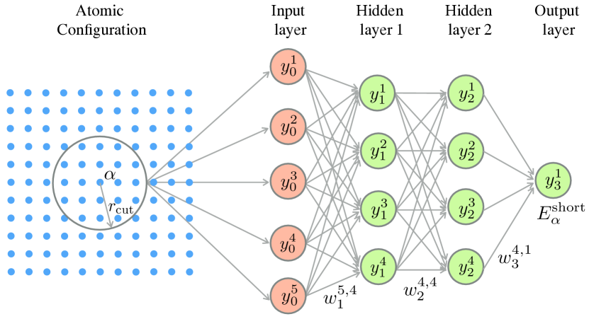
Figure 1: Schematic representation of an NN potential for the short-range energy $E_{\alpha}^{\text{short}}$ of atom $\alpha$. This NN consists of an input layer, two hidden layers, and an output layer. The configuration of neighbors of atom $\alpha$ within a cutoff $r_{\text{cut}}$ is transformed to a descriptor vector $y_{0}^{j}$ ($j=1,2,\dots,5$), which serves as the input to the NN. The arrows connecting nodes in adjacent layers represent weights. Biases and activation functions are not shown in this figure. See text for explanation of the variables.

Interatomic potentials must be invariant with respect to translation, rotation, and inversion of space, and permutation of chemically equivalent atoms [42]. To ensure that the NN satisfies these requirements, the environment of atom $\alpha$, which is the input to the NN, must be transformed to a new representation called a descriptor that automatically satisfies these invariances. Thus the input layer $\bm{y}_{0}$ is a descriptor vector which is a function of the set of positions $\bm{r}_{\alpha}^{\text{neigh}}$ of all atoms within the neighborhood of atom $\alpha$ defined by the cutoff distance $r_{\text{cut}}$ (including atom $\alpha$ itself), i.e.

$$y_{0}^{j}=g^{j}(\bm{r}_{\alpha}^{\text{neigh}}),$$ (7)

where $j$ ranges over the components of the descriptor vector.

Various types of descriptors have been proposed in recent years including the Coulomb matrix [30] and bag of bonds [43] for molecular systems, and the smooth overlap of atomic positions (SOAP) [44], symmetry functions [45], and moment tensor [32] for crystalline materials. In this work, we use symmetry functions [45, 46], which are discussed in detail in the Supplemental Material (SM) [41].

A challenging aspect of training an NN, which is also a source of the power and flexibility of the method, is that it is up to the developer to select the number of descriptor terms to retain, the number of hidden layers, the number of nodes within each hidden layer (which need not be the same), and the activation function. It is also possible to create different connectivity scenarios between layers. Here we have opted for simplicity and adopted a fully-connected network with the same number of nodes in each hidden layer to reduce the number of hyperparameters that need to be determined in the training process. We chose the commonly used hyperbolic tangent function, $\tanh(x)=(e^{x}-e^{-x})/(e^{x}+e^{-x})$, as the nonlinear activation function $h$.

II.2 Dataset

The hNN–Gr_x potential parameters were determined from a dataset of energies and forces for pristine and defected monolayer graphene, bilayer graphene, and graphite at various states. This includes configurations with compressed and stretched cells, random perturbations of atoms, and configurations drawn from ab initio molecular dynamics (MD) trajectories at different temperatures. The dataset consists of a total number of 14,250 configurations that are randomly divided into a training set of 13,500 configurations (95%) and a test set of 750 configurations (5%). The dataset along with a detailed description of the configurations are provided in the SM [41].

The dataset is generated from DFT calculations using the Vienna Ab initio Simulation Package (VASP) [47, 48]. The exchange-correlation energy of the electrons is treated within the generalized gradient approximated (GGA) functional of Perdew, Burke and Ernzerhof (PBE) [49]. For monolayer and bilayer graphene, the supercell size in the direction perpendicular to graphene planes is set to 30 Å to minimize the interaction between periodic images. The reciprocal space is sampled using the $\Gamma$-centered Monkhorst Pack grids [50] and the number of grids is chosen so that the energy is converged to $1~{}\text{meV/atom}$. The energy cutoff for the plane wave basis is set to $500~{}\text{eV}$. Standard density functionals such as the local density approximation (LDA) and GGA accurately represent Pauli repulsion in interlayer interactions, but fail to capture vdW forces that result from dynamical correlations between fluctuating charge distributions. To address this limitation, various approximate corrections have been proposed and we adopt the many-body dispersion (MBD) method [51], which has been shown to reproduce the more accurate adiabatic-connection fluctuation-dissipation theory based random-phase-approximation (ACFDT–RPA) and experimental results quite well [26].

II.3 Training

The hNN–Gr_x potential is fit in two stages: first the parameters in the long-range part in Eq. (2) are determined, then the parameters in the short-range NN part in Eq. (6).

For the long-range part, the interval bounds in the switching functions ($r_{\text{up}}^{\text{min}}$, $r_{\text{up}}^{\text{max}}$, $r_{\text{down}}^{\text{min}}$, $r_{\text{down}}^{\text{max}}$) are listed in Table 1. The $r_{\text{up}}^{\text{min}}$ and $r_{\text{up}}^{\text{max}}$ values are selected based on the graphene equilibrium lattice spacing of about 3.4 Å, $r_{\text{down}}^{\text{max}}$ sets the cutoff of the long-range interactions and is based on prior experience with DRIP [26], and $r_{\text{down}}^{\text{min}}$ is set a bit lower to create a smooth transition. After fixing these, a single parameter $\bm{\theta}=\{A\}$ remains to be determined. It is optimized by minimizing a loss function $L(\bm{\theta})$ that quantifies the difference between the predictions of Eq. (2) and DFT results for a subset of the training set comprised of AB-stacked bilayer graphene at various layer spacings ranging from $r_{\text{up}}^{\text{max}}$ to $r_{\text{down}}^{\text{min}}$. The subset consists of $M=52$ configurations with concatenated coordinates $\bm{r}_{m}$ for $m\in[1,M]$, such that $\bm{r}_{m}\in\mathbb{R}^{3N_{m}}$ where $N_{m}$ is the number of atoms in configuration $m$. The loss function is

$$L(\bm{\theta})= \sum_{m=1}^{M}\frac{1}{2}w^{\text{e}}_{m}\left[E(\bm{r}_{m};\bm{\theta})-E_{m}^{\text{DFT}}\right]^{2}$$

$$+ \sum_{m=1}^{M}\frac{1}{2}w^{\text{f}}_{m}\left\|\bm{f}(\bm{r}_{m};\bm{\theta})-\bm{f}_{m}^{\text{DFT}}\right\|^{2},$$ (8)

where $E(\bm{r}_{m};\bm{\theta})$ and $\bm{f}(\bm{r}_{m};\bm{\theta})=-\left.(\partial E/\partial\bm{r})\right|_{\bm{r}_{m}}\in\mathbb{R}^{3N_{m}}$ are the potential energy and concatenated forces for configuration $m$, in which $E(\bm{r}_{m};\bm{\theta})=E^{\text{long}}=\sum_{\alpha=1}^{N_{m}}E_{\alpha}^{\text{long}}$. The energy weight $w^{\text{e}}_{m}$ and force weight $w^{\text{f}}_{m}$ of configuration $m$ have units of eV^-2 and (eV/Å)^-2, respectively, given energy in units of eV and forces in units of eV/Å. We set $w^{\text{e}}_{m}$ to $1/(N_{m})^{2}$, and $w^{\text{f}}_{m}$ to $1/(10(N_{m})^{2})$. The target DFT energy and forces for the long-range part $E_{m}^{\text{DFT}}$ and $\bm{f}_{m}^{\text{DFT}}$ consider only interlayer interactions, obtained in the same way as described in detail in [26]. The resulting parameter $A$ is given in Table 1.

With the long-range interactions determined, the next step is to determine the short-range part of the potential. The same loss function in Eq. (II.3) is used with three differences compared with the long-range fitting: (1) the parameters $\bm{\theta}$ are the weights $\bm{W}$ and biases $\bm{b}$ in the NN; (2) the entire training set is used; and (3) the target energies $E_{m}^{\text{DFT}}$ and forces $\bm{f}_{m}^{\text{DFT}}$ are the differences between the total DFT values and the predictions from the long-range contribution in Eq. (2). The third item ensures that the potential produces correct total energy and forces when the long-range and short-range parts are used together.

The optimization was carried out using the KIM-based Learning-Integrated Fitting Framework (KLIFF) [52] with an L-BFGS-B minimizer [53]. KLIFF is compatible with potentials conforming to the Knowledgebase of Interatomic Models (KIM) application programming interface (API) [54]. See the SM [41] (also, references[55, 56, 57, 58] therein) for more details on KIM and how to use KIM potentials. A grid search was performed to determine the optimal number of hidden layers and nodes by fitting the potential to the training set in each case and finding which provided the minimum loss for the test set. Using this process, it was found that 3 hidden layers with 30 nodes per layer was the optimal choice. The resulting energy root-mean-square error (RMSE) and forces RMSE for the test set are 4.66 meV/atom and 41.41 meV/(Å atom), respectively, and 4.56 meV/atom and 41.13 meV/(Å atom) for the training set. See Table 1 for details of the NN parameters.

III Testing of the hNN–Gr_x potential

An extensive set of calculations were performed to test the ability of the new hNN–Gr_x potential to reproduce structural, energetic, and elastic properties of monolayer graphene, bilayer graphene, and graphite obtained from DFT. A portion of the results is presented in Table 2 together with results from widely used potentials, ab initio ACFDT–RPA, and experiments.

Table 2: Summary of structural, energetic, and elastic properties computed from the new hNN–Gr_x potential and other widely used potentials. The properties include in-plane lattice parameter of monolayer graphene, $a$; equilibrium layer spacing of bilayer graphene in AB stacking, $d_{\text{AB}}$, bilayer graphene in AA stacking, $d_{\text{AA}}$, and graphite, $d_{\text{graphite}}$; interlayer binding energy of bilayer graphene, $E_{\text{AB}}$; cohesive energy of monolayer graphene, $E_{\text{coh}}$; single-vacancy formation energy in monolayer graphene, $E_{\text{v}}$; and elastic moduli of graphite (outside parentheses) and monolayer graphene (in parentheses). Also included are some first-principles and experimental results, as well as the computational expense relative to Tersoff. Notes: (1) Since the Tersoff, REBO, and GAP–Gr (GAP for graphene) potentials lack the ability to model interlayer interactions (see Section I), they do not have predictions for properties related to interlayer interactions. (2) The KC and DRIP potentials only model interlayer interactions and therefore cannot be used to compute the in-plane lattice parameter. Results from these potentials used an in-plane lattice parameter of $a=2.46~{}\text{\AA}$. For elastic properties, only the modulus related to stretching perpendicular to the layers is computed in this case.

Method	$a$	$d_{\text{AB}}$	$d_{\text{AA}}$	$d_{\text{graphite}}$	$E_{\text{AB}}$	$E_{\text{coh}}$	$E_{\text{v}}$	$C_{11}$	$C_{12}$	$C_{13}$	$C_{33}$	$C_{44}$	Time
	(Å)	(Å)	(Å)	(Å)	(eV/atom)	(eV/atom)	(eV)	(GPa)	(GPa)	(GPa)	(GPa)	(GPa)	(relative)
hNN–Grx (present)	2.467	3.457	3.618	3.402	21.63	8.07	8.08	978.31 (1061.83)	176.54 (208.77)	$-66.74$	40.35	1.79	279.4
AIREBO [20]	2.419	3.392	3.416	3.358	23.61	7.43	7.94	1153.50 (1162.46)	144.87 (147.64)	0.08	40.40	0.28	4.5
AIREBO–M [23]	2.420	3.299	3.324	3.294	16.18	7.42	7.93	1174.25 (1157.43)	147.66 (146.23)	-0.02	35.72	0.28	4.9
LCBOP [22]	2.459	3.346	3.365	3.346	12.52	7.35	8.13	1049.91 (1054.32)	157.29 (159.03)	0.04	29.80	0.23	1.6
ReaxFF [25]	2.462	3.285	3.294	3.260	34.59	7.52	7.52	1147.67 (1119.84)	831.84 (811.43)	$-0.77$	34.41	0.15	26.1
Tersoff [17]	2.530					7.39	7.12	(1274.00)	($-240.11$)				1
REBO [19]	2.460					7.39	7.82	(1059.25)	(148.33)				1.6
GAP–Gr [38]	2.467					7.96	6.55	(1108.81)	(212.19)				3814.7
KC [12]		3.374	3.602	3.337	21.60						34.45		36.6
DRIP [26]		3.439	3.612	3.415	23.05						32.00		35.5
DFT(PBE+MBD)	2.466	3.426	3.641	3.400	22.63	8.06	7.93	1080.12 (1084.41)	162.25 (161.25)	$-4.63$	33.18	3.32	$\sim 10^{7}$
ACFDT–RPA		3.39		3.34							36
Experiment	2.46			3.34				1060 (1018)	180	15	36.5	0.27
	2.46			3.356				1109	139	0	38.7	4.95

The in-plane lattice parameter of monolayer graphene, $a$, is obtained by fitting the Birch–Murnaghan equation of state (EOS) [66] (to conform to the approach used in DFT computations). The results presented in Table 2 show that AIREBO and AIREBO–M underestimate the value of $a$, Tersoff overestimates it, and the other potentials give values close to the experimental and DFT results. Table 2 also shows the values of the equilibrium layer spacing for bilayer graphene in AB stacking $d_{\text{AB}}$, bilayer graphene in AA stacking $d_{\text{AA}}$, and graphite $d_{\text{graphite}}$. These values are also obtained from the Birch–Murnaghan EOS, keeping the in-plane lattice parameter fixed to its equilibrium monolayer value. The hNN–Gr_x potential and DRIP are in good agreement with DFT(PBE+MBD) results to which they were fit. The KC model is in better agreement with more accurate ACDFT–RPA. The remaining potentials all underestimate the AA separation, and have inconsistent results for AB and graphite: AIREBO and LCBOP are accurate for both, and AIREBO–M and ReaxFF underestimate both. Given this it is not surprising that except for hNN–Gr_x, KC, and DRIP, all of the above potentials provide inaccurate values for $d_{\text{AA}}-d_{\text{AB}}$. The DFT value is 0.215 Å, and the potentials predict: 0.024 Å (AIREBO), 0.025 Å (AIREBO–M), 0.019 Å (LCBOP), and 0.009 Å (ReaxFF). The reason for the poor accuracy is that these potentials cannot distinguish the AA and AB stacking states. This is discussed further below.

Next, we consider energetics. The interlayer binding energy of a graphene bilayer $E_{\text{b}}$ as a function of layer spacing $d$ is shown in Fig. 2 for AB and AA stacking. The curves are shifted such that $\Delta E=E_{\text{b}}-E_{\text{AB}}$ and $\Delta d=d-d_{\text{AB}}$, where $E_{\text{AB}}$ (listed in Table 2) is the interlayer binding energy of AB-stacked bilayer graphene at the equilibrium layer spacing $d_{\text{AB}}$ (i.e. $E_{\text{AB}}$ is the depth of the energy well relative to a reference state at infinite separation). We see that the AIREBO, AIREBO–M, LCBOP, and ReaxFF potentials give nearly identical results for energy versus separation in the AB and AA stacking states in contrast to DFT where a clear difference exists. In addition, the AIREBO–M and LCBOP potentials underestimate the depth of the energy wells, whereas the ReaxFF potential overestimates it. (This can be seen by considering the values predicted by these potentials relative to DFT at the largest separation of $\Delta d=2.5$ Å, which is approaching the reference state). The hNN–Gr_x potential correctly captures the energy difference between the AB and AA stacking states as well as the depth of the energy wells. KC and DRIP can also capture the energy difference (see [26]). Also notable is that at large separation, the curves for the two stacking states merge since registry effects due to $\pi$-orbital overlap become negligible and interlayer interactions are dominated by dispersion attraction. This effect is captured correctly by the hNN–Gr_x potential.

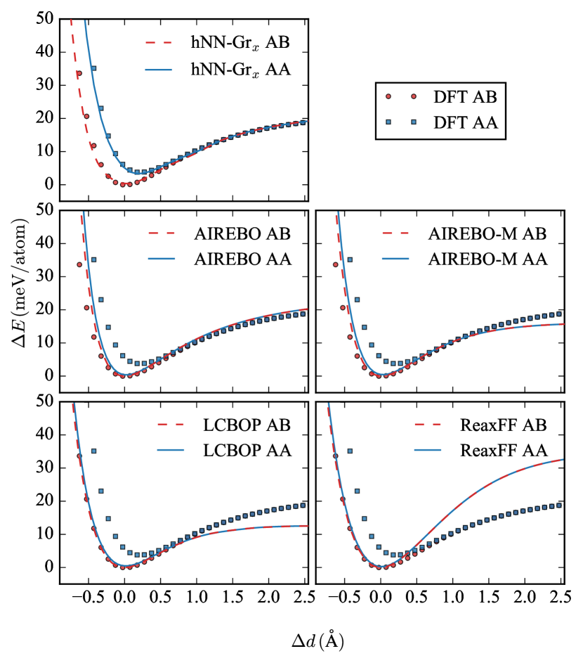
Figure 2: Interlayer binding energy of a graphene bilayer versus layer spacing for AB and AA stackings obtained from various potentials compared with DFT results. The curves are shifted such that the minimum energy in AB stacking is located at (0, 0).

A more complete view of the interlayer energetics is obtained by considering the generalized stacking fault energy (GSFE) surface obtained by sliding one layer relative to the other while keeping the layer spacing fixed. Fig. 3 shows the results for a layer spacing of $d=3.4~{}\text{\AA}$; the hNN–Gr_x potential is in quantitative agreement with DFT results. The KC and DRIP GSFEs have a similar appearance (see [26]), whereas the AIREBO, AIREBO–M, LCBOP, and ReaxFF GSFEs are nearly flat (not shown).

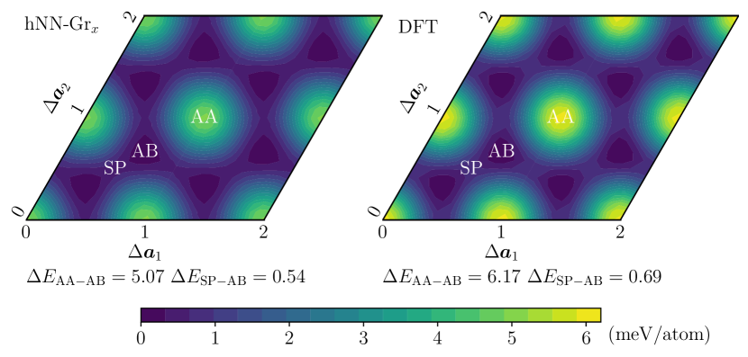
Figure 3: The GSFE of bilayer graphene obtained by sliding one layer relative to the other at a fixed layer spacing of $d=3.4~{}\text{\AA}$. The energy is relative to the AB state, which is $-21.53~{}\text{meV/atom}$ for the new hNN–Gr_x potential (on the left) and $-22.33~{}\text{meV/atom}$ for DFT (on the right). $\Delta E_{\text{AA-AB}}$ denotes the energy difference between the AA and AB states, and similarly $\Delta E_{\text{SP-AB}}$ denotes the energy difference between saddle point (SP) and AB states. The sliding parameters $\Delta\bm{a}_{1}$ and $\Delta\bm{a}_{2}$ are in units of lattice parameter $a=2.466~{}\text{\AA}$.

Also listed in Table 2 are the cohesive energy $E_{\text{coh}}$ and relaxed single-vacancy formation energy $E_{\text{v}}$ for monolayer graphene. The latter is computed as $E_{\text{v}}=E_{2}-E_{1}-\mu$, where $E_{1}$ and $E_{2}$ are the relaxed energy of monolayer graphene before and after the single vacancy is created (by removing an atom from the simulation cell), and $\mu$ is the chemical potential of carbon, taken to be the cohesive energy $E_{\text{coh}}$ here. All potentials perform reasonably well for these two properties except that the single-vacancy formation energy predicted by GAP–Gr is significantly smaller compared with the other potentials and DFT. This is likely because GAP–Gr was only trained against configurations drawn from MD trajectories of ideal graphene.

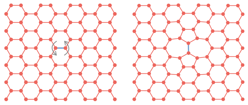
(a)

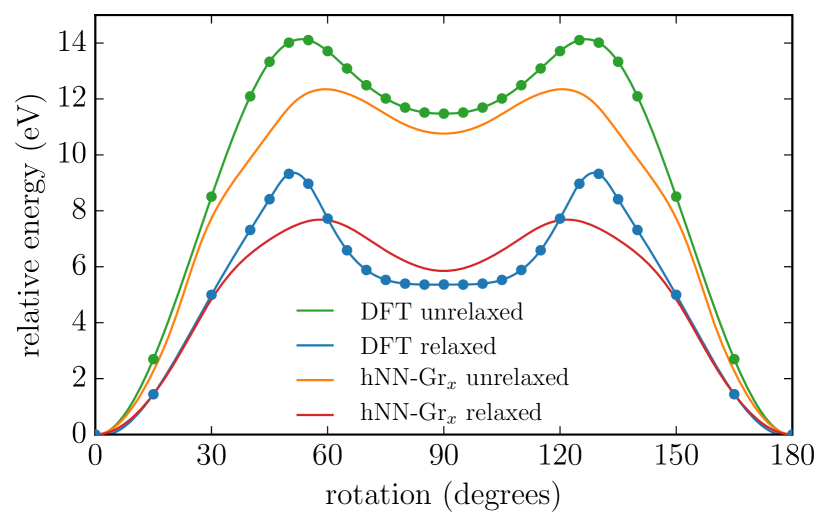
(b)

Figure 4: Stone–Wales defect created by rotating a pair of atoms. (a) Monolayer graphene with a pair of atoms rotated at angles $0^{\circ}$ (on the left) and $90^{\circ}$ (on the right), and (b) energy versus rotation for both relaxed and unrelaxed structures predicted by DFT and the hNN–Gr_x potential.

Another interesting example, which tests the ability of the hNN–Gr_x potential to capture changes in hybridization, is the concerted exchange mechanism first studied in graphene by Kaxiras and Pandey [67]. In this process a pair of atoms rotate by 90 degrees converting four hexagonal rings to two pentagons and two heptagons thereby creating a Stone–Wales (SW) defect (see Fig. 4(a)). To explore the energetics of the process, the total energy of a system of 96 atoms was computed as a function of the rotation angle using DFT and the hNN–Gr_x potential. At each angle, the energy is minimized with respect to the positions of the atoms subject to the constraint that the two rotating atoms can only move along the line connecting them (i.e. along the blue line shown in Fig. 4(a)).

The energy versus rotation curves for DFT and hNN–Gr_x are shown in Fig. 4(b), where the DFT results are interpolated by a cubic spline. Overall the hNN–Gr_x results follow the DFT curve, predicting a SW defect formation energy of 5.85 eV (red curve at rotation $90^{\circ}$), about 9% higher than the DFT prediction of 5.37 eV (blue curve at rotation $90^{\circ}$). The energy barriers at the transition state are 7.68 eV at a rotation of $58^{\circ}$ for hNN–Gr_x, and 9.32 eV at a rotation of $51^{\circ}$ for DFT, a relative difference of about 17.6%. Since hNN–Gr_x is a machine learning potential, the accuracy can be systematically improved by augmenting the training set with configurations along the concerted exchange path. As a comparison, we also computed the energy versus rotation using the other potentials listed in Table 2 (see the results in the SM [41]). None of the potentials are in very good agreement with DFT, in particular, none capture the energy plateau in the vicinity of the SW defect.

Finally, we consider elasticity properties. The elastic moduli of hexagonal graphite was computed using finite differences. The five independent components are listed in Table 2. For each potential, the graphitic structure is constructed using its corresponding in-plane lattice parameter, $a$, and equilibrium layer spacing $d_{\text{graphite}}$. In addition, the in-plane elastic moduli $C_{11}$ and $C_{12}$ of monolayer graphene were computed (values listed in parentheses). Similar to graphite, the graphene structure is constructed using the corresponding in-plane lattice parameter of each potential, whereas the “thickness” of graphene (required to obtain bulk units) is assumed to be $3.34~{}\text{\AA}$ in all cases. The results show that for graphite the hNN–Gr_x potential is in good agreement with DFT for $C_{11}$ (9.5%) and $C_{12}$ (8.8%), reasonable agreement for $C_{33}$ (21.6%) and $C_{44}$ (46.1%), and incorrect for $C_{13}$ (1340%) (although we note that the DFT results disagree with experiments in this case). For graphene, the hNN–Gr_x potential is in excellent agreement for $C_{11}$ (2.1%), but overestimates $C_{12}$ (29.5%). For the other potentials, notable disagreements are: (1) ReaxFF predicts significantly larger values of $C_{12}$ of both graphite and graphene; (2) All of the potentials greatly underestimate $C_{44}$ for graphite; (3) Tersoff overestimates $C_{11}$ and predicts negative $C_{12}$ for graphene; and (4) GAP–Gr overestimates $C_{12}$ for graphene.

While the elastic moduli provide insight into the elastic behavior of the potentials, a more complete view is gained from the phonon dispersion curves. A number of thermodynamic properties, such as the thermal expansion coefficient and heat capacity, can be obtained directly from dispersion relations via calculation of the free energy. Fig. 5 shows the phonon dispersion curves of monolayer graphene calculated using finite differences as implemented in the phonopy package [68]. The predictions of the hNN–Gr_x potential and GAP–GR are in excellent agreement with DFT. The other potentials provide good agreement for some phonon branches, but not all. REBO quantitatively predicts the shape and dispersion character of most of the phonon branches, but fails for the high-frequency transverse optical (TO) and longitudinal optical (LO) branches. LCBOP, AIREBO, AIREBO–M, and ReaxFF are comparable, qualitatively predicting the overall shapes of most curves, but are in poor quantitative agreement with DFT. Tersoff has the worst performance with poor qualitative agreement for most branches. We note that a drawback common to all of the physics-based potentials is that they fail to capture the dispersive behavior of the high-frequency LO and TO branches, which hNN–Gr_x and GAP–Gr predict with negligible error. The phonon dispersions of bilayer graphene and graphite (not shown here) are identical to monolayer graphene, except that the ZA branch splits into two doubly degenerate branches near the $\Gamma$ point [69, 70].

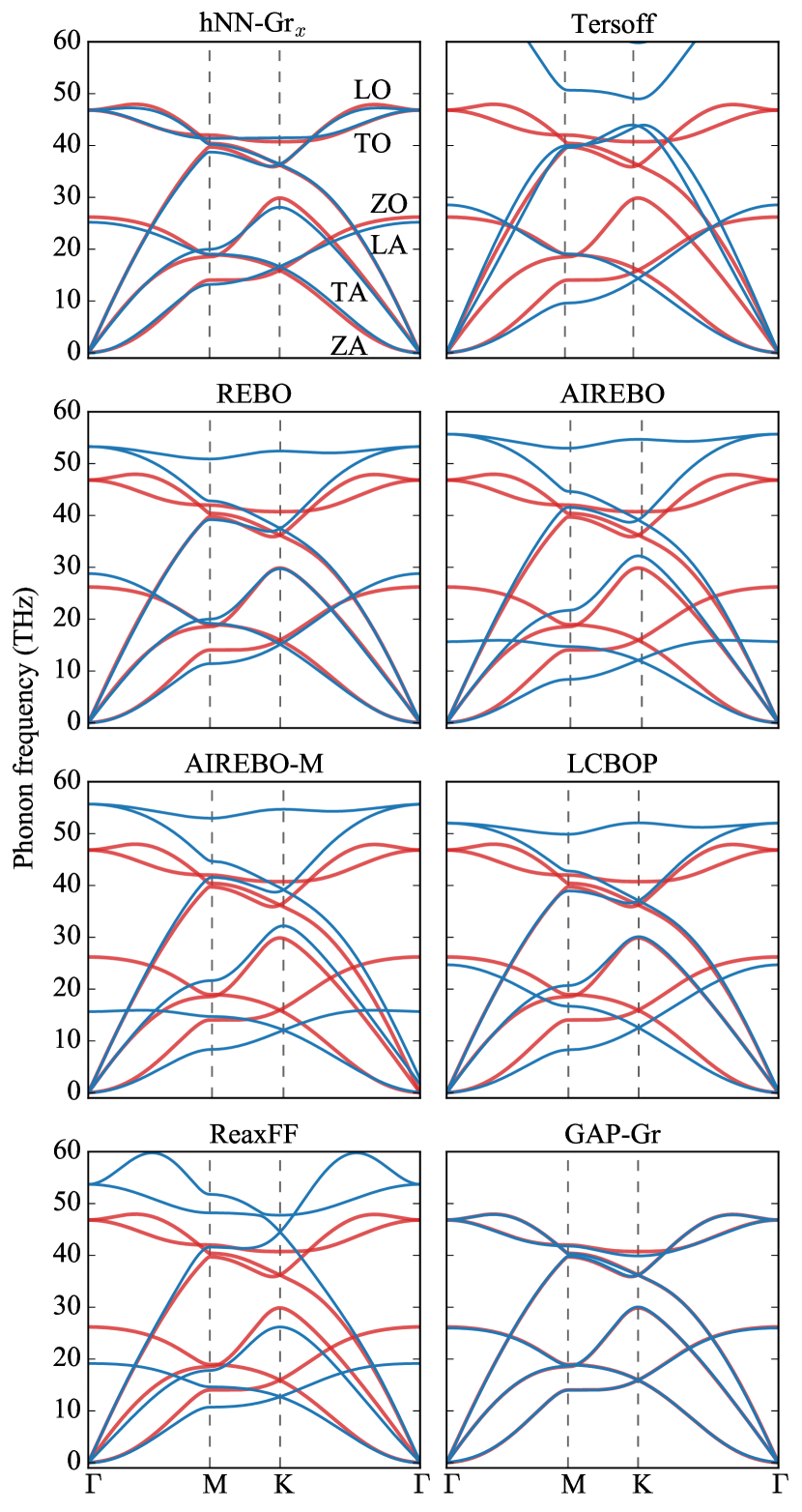
Figure 5: Phonon dispersion curves of monolayer graphene along high-symmetry points in the first Brillouin zone. The red curve is the DFT prediction, and the blue curves are results from the potentials. Branch labels are shown in the upper left panel, where “L” stands for longitudinal, “T” for transverse, “Z” for flexural, “O” for optical, and “A” for acoustic. Note that parts of the highest two branches by the Tersoff potential are not shown.

For the properties computed above and the potentials tested, the results indicate that overall, machine learning potentials (both hNN–Gr_x and GAP–Gr) have higher accuracy than the physics-based potentials. However, the accuracy comes at the price of increased computational cost. Table 2 shows the time (relative to Tersoff) that it takes each potential to complete an MD trajectory of the same duration under the canonical ensemble. The simulations were carried out using LAMMPS [55, 71] with hNN–Gr_x implemented in KIM [54, 72], GAP–Gr implemented in QUIP [73], and the other potentials natively built into LAMMPS. While GAP–Gr is nearly 4000 times slower than Tersoff, the hNN–Gr_x potential is much faster, only about 280 times slower than Tersoff. As discussed in I, this is a benefit of parametric methods; the evaluation time does not depend on the size of the training set. Both hNN–Gr_x and GAP–Gr are still significantly faster than a first-principles method like DFT, although they are significantly slower than the tested physics-based potentials. KC and DRIP are relatively more expensive than the other physics-based potentials because to model long-range dispersion attraction, they need to use a much larger cutoff distance. For example, DRIP uses a cutoff of 12 Å, whereas the other physics-based potentials considered here typically have cutoffs smaller than 5 Å.

IV Applications

The new hNN–Gr_x potential is applied to two problems of interest that are beyond the capabilities of DFT: (1) thermal conductivity of monolayer graphene; and (2) interlayer friction in bilayer graphene. In both cases the effect of vacancies on the results are explored.

IV.1 Thermal conductivity

Graphene has been reported to have extremely high thermal conductivity with experimentally measured values between 1500 and 2500 W/mK [74, 75, 76, 77, 78] in suspended samples at room temperature. (For comparison, copper has a thermal conductivity of about 400 W/mK.) Despite these efforts, accurate determination of the thermal conductivity of graphene remains challenging because thermal transport in this material is very sensitive to defects and experimental conditions [79, 80]. Atomistic simulations using interatomic potentials provide an alternative approach to study the thermal conductivity in graphene and investigate the effect of defects. One concern is that interatomic potentials do not account for electron contributions to thermal transport which are the dominant effect in metals. Fortunately, although graphene is a semi-metal, at room temperature lattice vibrations account for the majority of the thermal transport making the interatomic potential estimate meaningful [81, 82]. An accurate prediction of the lattice contribution depends on the ability of the potential to describe the phonon dispersion curves, and in particular the ZA mode associated with out-of-plane vibrations that provides the dominant contribution to the lattice thermal conductivity in suspended graphene [83, 84]. As seen in Fig. 5, the hNN–Gr_x potential is highly accurate in predicting all phonon dispersion branches including ZA.

The thermal conductivity is computed using the Green–Kubo method, an equilibrium MD approach. The Green–Kubo expression, based on linear-response theory, is [85, 86]

$$\kappa_{ij}=\frac{1}{\Omega k_{\text{B}}T^{2}}\int_{0}^{\infty}\langle J_{i}(t)J_{j}(0)\rangle\,\text{d}t,$$ (9)

where $i,j\in\{x,y,z\}$ are Cartesian components, $k_{\text{B}}$ is Boltzmann’s constant, $T$ is the temperature, $\langle J_{i}(t)J_{j}(0)\rangle$ is the heat current auto-correlation (HCA) function expressed as a phase average, and $\Omega$ is the volume of the system defined as the area of graphene multiplied by the van der Waals thickness (3.457 Å in the present case; see Table 2). The upper limit of the integral in Eq. (9) can be approximated by $t_{P}$, the correlation time required for the HCA to decay to zero. In the case of an MD simulation, the phase average in the HCA is approximated by a time average computed at discrete MD time steps. Consequently, Eq. (9) is in fact a summation and we actually compute [86]

$$\kappa_{ij}(t_{P})=\frac{\Delta t}{\Omega k_{\text{B}}T^{2}}\sum_{p=1}^{P}(Q-p)^{-1}\sum_{q=1}^{Q-p}J_{i}(p+q)J_{j}(q),$$ (10)

where $\Delta t$ is the MD time step, $Q$ is the total number of steps, $P=t_{P}/\Delta t$ is the number of steps for integration (should be smaller than $Q$), and $J_{i}(p+q)$ is the $i$th component of the heat current at step $p+q$.

A key component of the Green–Kubo method is the definition of the heat current. We note that the heat current implemented in the LAMMPS MD code [55, 71] is intended for pair potentials only. For many-body potentials, such as the hNN–Gr_x potential, using the LAMMPS expression can lead to incorrect results. In this work, we use the definition in [88], which applies to arbitrary many-body potentials.

Figure 6: Thermal conductivity in the $x$ direction, $\kappa_{xx}$, as a function of $t_{P}$ for pristine graphene, graphene with 0.1% vacancy density, and graphene with 0.2% vacancy density. In each panel, the thin gray lines are the HCA cumulative averages obtained from eight independent trajectories, and the thick lines (red, blue, or green) are the means of these HCA curves. The “X” denotes the sample with the largest $\kappa_{xx}$ at $t_{P}=1~{}\text{ns}$ among the eight samples whose normalized HCA is shown in Fig. 7.

We study the thermal conductivity in pristine graphene and investigate the impact of defects. In practice, graphene can contain a variety of defects including single vacancies, double vacancies, Stone–Wales defects, adatoms, dislocations, and grain boundaries [89, 90]. Here, we focus on single vacancies, which have been experimentally shown to be a common type of defect in graphene [91]. The base graphene system consists of a periodic rectangular supercell of size 51.25 Å by 49.32 Å in the $x$ (armchair) and $y$ (zigzag) directions comprised of 960 atoms. Separate calculations showed that this system is sufficiently large to obtain converged thermal conductivity for ideal graphene in agreement with previously published results in [84]. Single vacancies are generated by randomly removing atoms from the supercell. The equations of motion are integrated using a velocity-Verlet algorithm with a time step of $\Delta t=1~{}\text{fs}$. The system is initially thermalized for 0.5 ns at a constant temperature of $T=300~{}\text{K}$ under $NVT$ conditions (canonical ensemble) using a Langevin thermostat. The thermostat is then switched off and data for the Green–Kubo expression is collected under $NVE$ conditions (microcanonical ensemble). A time scale on the order of nanoseconds is necessary to sufficiently converge the HCA function [86]. We ran the NVE simulation for 10 ns based on previous studies of thermal conductivity in graphene [92, 93].

The thermal conductivity in the $x$ (armchair) direction, $\kappa_{xx}$, as a function of $t_{P}$ for pristine graphene, graphene with a 0.1% vacancy density (one vacancy per supercell), graphene with a 0.2% vacancy density (two vacancies per supercell) is plotted in Fig. 6. In each case, the thermal conductivity is computed by averaging over eight uncorrelated trajectories with different initial conditions. We see that the majority of the samples are well converged after $t_{P}=0.5~{}\text{ns}$, with the mean showing an even better convergence. The thermal conductivity of pristine graphene measured at $t_{P}=0.5~{}\text{ns}$ is 2531 W/mK, in good agreement with the experimental values of 1500–2500 W/mK for suspended graphene [74, 75, 76, 77, 78]. The thermal conductivity for the graphene with a 0.1% vacancy density is 415 W/mK, an 84% reduction, and for graphene with a 0.2% vacancy density it is 195 W/mK, a 92% reduction. Similar values were obtained in the $y$ (zigzag) direction, i.e. $\kappa_{yy}\approx\kappa_{xx}$ as expected due to isotropy in the graphene plane.

In Fig. 7, we plot the normalized HCA, $\left<J_{x}(t)J_{x}(0)\right>/\left<J_{x}(0)J_{x}(0)\right>$, for the samples marked with an “X” in Fig. 6. It is clear that the normalized HCA decays to zero much earlier than $t=0.5~{}\text{ns}$ for all three types of graphene, indicating that $t_{P}=0.5~{}\text{ns}$ is sufficient for calculating the thermal conductivity. Further, the decay of the normalized HCAs for graphene containing vacancies is much faster than that of pristine graphene, which is related to the fact that the thermal conductivity in defective graphene is much smaller than in pristine graphene. (Note that $\left<J_{x}(0)J_{x}(0)\right>$ is almost the same for all three cases and thermal conductivity is the integral of the HCA). The underlying mechanism for the reduced thermal conductivity of graphene with vacancies is that vacancy defects are a strong scattering source for phonons, which govern heat transport in this system. Creation of a single vacancy leaves three carbon atoms with two-fold coordination, effectively breaking the $sp^{2}$ characteristics of the local lattice. These two-fold coordinated atoms are less likely to follow the normal pattern of vibrations in pristine graphene and cause a significant degree of scattering [93].

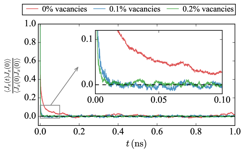
Figure 7: Normalized HCA, $\left<J_{x}(t)J_{x}(0)\right>/\left<J_{x}(0)J_{x}(0)\right>$, as a function of time $t$ for pristine graphene, graphene with 0.1% vacancy density, and graphene with 0.2% vacancy density. The red, blue, and green curves are for the samples marked with an “X” for graphene with 0, 0.1% and 0.2% vacancy density in Fig. 6.

IV.2 Interlayer Friction

Although the bonding between layers in multilayer graphene is weak, the material still exhibits significant resistance to sliding due to orbital overlap between layers. The friction becomes even larger when covalent bonds are formed between adjacent layers. Such bonds have been proposed to occur when vacancies exist in close proximity to each other in the top and bottom layers and react to form covalent bonds in their vicinity [94]. A plausible mechanism for this to happen is the creation of vacancies through high-energy ion or electron bombardment of multilayer graphene [95]. Here, we study the effect of vacancies and interlayer covalent bonding on friction in bilayer graphene.

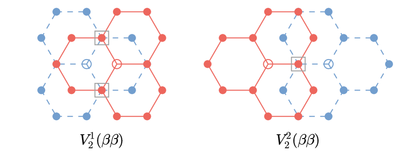
Figure 8: Close-proximity divacancies in adjacent layers of AB-stacked bilayer graphene that favor the formation of covalent bonds between layers. Hollow circles denote vacancies, and gray squares are locations where covalent bonds can form between atoms in adjacent layers. (There are two atoms in each gray square; the blue atom in the bottom layer is hidden by the red atom in the top layer.) Following the notation in [94], the subscript 2 in $V_{2}^{1}(\beta\beta)$ and $V_{2}^{2}(\beta\beta)$ indicates that two single vacancies form a divacancy, the superscripts 1 and 2 denote first- and second-nearest interlayer neighbors, and $\beta$ means that a vacancy is located at the hexagonal ring center of the other layer.

A number of possible interlayer divacancies can form via the coalescence of single vacancies in adjacent layers leading to the formation of covalent bonds [94, 96]. We focus on the two structures shown in Fig. 8, where the two vacancies are first- and second-nearest interlayer neighbors referred to as $V_{2}^{1}(\beta\beta)$ and $V_{2}^{2}(\beta\beta)$ (see the figure caption for an explanation of the notation).

Graphene bilayers containing the two types of divacancies $V_{2}^{1}(\beta\beta)$ and $V_{2}^{2}(\beta\beta)$ are fully relaxed using DFT and the hNN–Gr_x potential. An important point is that in order for covalent bonds to form between layers it is necessary to compress the bilayer in the direction perpendicular to the layers, so that the layers are brought to within a spacing of about $2.4~{}\text{\AA}$ prior to relaxation. Both DFT and the hNN–Gr_x potential predict the same core structure after relaxation as shown in Fig. 9. Two interlayer covalent bonds of equal length (colored green) are formed in the first-nearest-neighbor divacancy ($V_{2}^{1}(\beta\beta)$). The bond length is predicted by the hNN–Gr_x potential to be 1.44 Å, which is good agreement with the DFT value of 1.53 Å. The formation of the covalently-bonded divacancy leaves a two-fold coordinated atom in each layer, which is electronically unsaturated and could be chemically active. For the second-nearest-neighbor divacancy ($V_{2}^{2}(\beta\beta)$) only one bridging bond is formed with a length of 1.40 Å according to the hNN–Gr_x potential. Again there is good agreement with DFT, which predicts a bond length of 1.38 Å. As expected the single bond is stronger than the pair of bonds for the first-nearest-neighbor divacancy as demonstrated by the shorter bond length in this case. The $V_{2}^{2}(\beta\beta)$ divacancy leaves two two-fold coordinated atoms in each layer, which reconstruct to form a bond (not shown) with a bond length predicted to be 1.84 Å by hNN–Gr_x and 2.15 Å by DFT. (The two atoms are 2.466 Å away from each other in pristine graphene.)

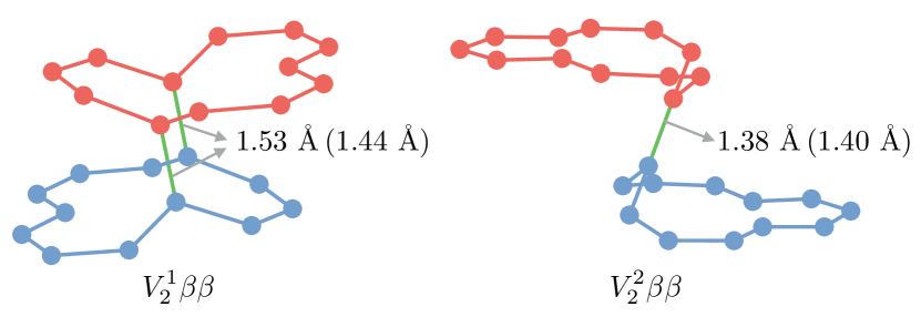
Figure 9: Core structures of the $V_{2}^{1}(\beta\beta)$ and $V_{2}^{2}(\beta\beta)$ divacancies after relaxation. The interlayer covalent bond(s) formed near the divacancy are colored green. The bond length predicted by DFT (hNN–Gr_x) is shown.

Next, we measure the interlayer friction force in bilayer graphene with and without the two types of divacancies. The setup for this simulation is shown in Fig. 10 for the armchair direction. A graphene layer (red) is placed on top of a larger layer (blue) and pulled to the right under displacement control conditions. The bottom layer has a width of 76.88 Å (in the $x$ direction) and height 22.19 Å (in the $y$ direction) and contains 648 atoms. The top layer has a width of 49.83 Å and 432 atoms. When divacancies are included, they are introduced into the center of the bilayer at the location indicated by the black rectangle in Fig. 10. Periodic boundary conditions are applied in the $x$ and $y$ directions, and the direction perpendicular to the plane is free. Thus the system corresponds to an infinite graphene nanoribbon with finite width in the $x$-direction (top layer) sliding on an infinite graphene layer (bottom). The atoms at the right end of the top layer (green shaded region) are displaced in the $x$ direction with a step size of 0.1 Å. At each step, after applying the displacement to these atoms, the total energy of the system is minimized subject to the following constraints: (1) The atoms at the right end of the bottom layer are fixed in all three directions; and (2) the $x$ coordinates of the atoms at the right end of the top layer are fixed to their displaced positions. Following relaxation, the force $F$ required to hold the top layer in its displaced position is computed as the total force acting on the constrained atoms in the top layer. From this the shear stress is computed as $\tau=F/A$, where $A$ is the area of the top layer. The shear stress is a more useful property than the force since it can be more readily compared across systems.

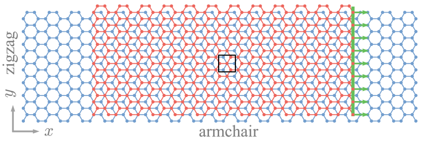
Figure 10: Representation of the simulation supercell used to compute the friction force in bilayer graphene with and without covalently-bonded divacancies in adjacent layers. The force required to pull the top layer to the right along the armchair direction is measured. The black rectangle indicates the location of divacancies when included.

Fig. 11(a) shows $\tau$ as a function of the pulling distance $\Delta x$ along the positive armchair direction. For a pristine bilayer without vacancies, the maximum shear stress is 423 MPa at $\Delta x=0.6~{}\text{\AA}$ with a periodicity of $\sqrt{3}a=4.27~{}\text{\AA}$ reflecting the underlying periodic nature of the bilayer structure. Note that the shear stress is negative once the top layer passes the unstable equilibrium state where it is balanced between forces pulling it forward and backwards. The maximum shear stress for $V_{2}^{1}(\beta\beta)$ is 1014 MPa at $\Delta x=2.9~{}\text{\AA}$. The interlayer bond breaks immediately once the shear stress reaches this maximum, leading to an abrupt drop in the shear stress. In contrast for the $V_{2}^{2}(\beta\beta)$ divacancy, the interlayer bond does not break at the maximum shear stress of 597 MPa at $\Delta x=0.8~{}\text{\AA}$, but instead breaks later at a somewhat lower shear stress at $\Delta x=2.2~{}\text{\AA}$. Once the interlayer bonds are broken, the $V_{2}^{1}(\beta\beta)$ and $V_{2}^{2}(\beta\beta)$ curves follow the pristine bilayer curve almost identically. This suggests that the presence of single vacancies in the layers (in the absence of interlayer covalent bonding) has a negligible effect on friction.

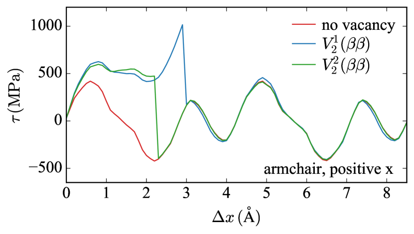
(a)

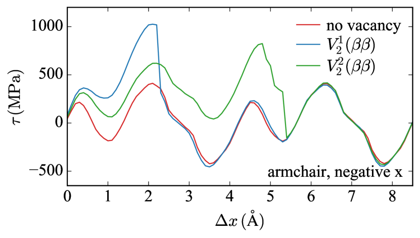
(b)

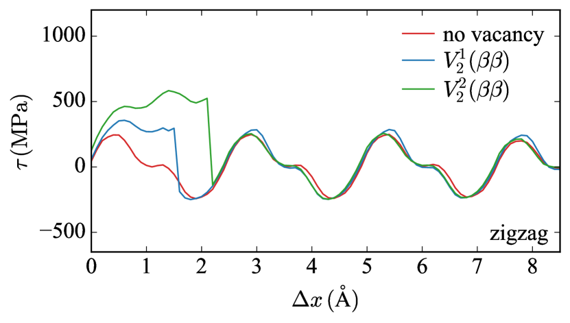
(c)

Figure 11: Shear stress $\tau$ versus pulling distance $\Delta x$ for bilayer graphene with and without divacancies. Three different pulling directions are shown (see Fig. 10): (a) and (b) armchair edge in the positive and negative $x$ directions, and (c) zigzag edge in the $y$ direction (positive and negative are the same).

We expect the shear stress for pristine graphene to depend on the pulling direction due to the changing crystallographic orientation. The effect of the divacancies will also depend on orientation. For example, referring to Fig. 8, we see that when pulling the top layer to the right, the single vacancies in $V_{2}^{1}(\beta\beta)$ move apart, whereas when pulling to the left they initially move closer together. We explore friction anisotropy by considering two more directions in Fig. 10: (1) pulling to the left along the armchair direction, and (2) pulling upwards along the zigzag direction (downwards is the same due to symmetry). In the first case, the simulation setup is the same as in Fig. 10, except that the atoms on the left end of the top layer are pulled in the negative $x$ direction. In the second case, a bilayer is constructed with similar geometry to Fig. 10, but with the zigzag edge aligned with the $x$ direction and the armchair edge aligned with the $y$ direction. This system contains 370 atoms in the top layer and 560 atoms in the bottom layer.

The shear stress versus pulling distance for these two cases are shown in Figs. 11(b) and 11(c). The results in the negative armchair direction (Fig. 11(b)) are similar to those in the positive armchair direction (Fig. 11(a)), but with some differences. The maximum shear stress for pristine graphene is the same as in Fig. 11(a) due to symmetry, but for $V_{2}^{1}(\beta\beta)$ it is 1018 MPa at $\Delta x=2.2~{}\text{\AA}$, which is still larger than that for $V_{2}^{2}(\beta\beta)$, 824 MPa at $\Delta x=4.8~{}\text{\AA}$. However, in this orientation $V_{2}^{1}(\beta\beta)$ breaks earlier (and immediately as before), whereas $V_{2}^{2}(\beta\beta)$ exhibits a large amount of slip prior to bond failure. For the zigzag direction in Fig. 11(c), the shear stress for pristine bilayer has a periodicity of 2.466 Å (smaller than that in Fig. 11(a) and Fig. 11(b)). The maximum shear stress for the pristine bilayer, $V_{2}^{1}(\beta\beta)$, and $V_{2}^{2}(\beta\beta)$ are 248 MPa, 352 MPa, and 583 MPa, respectively, all smaller than their counterparts in Fig. 11(a) and Fig. 11(b). This direction has the lowest friction resistance.

V Summary

We have developed a hybrid NN interatomic potential for multilayer graphene structures called “hNN–Gr_x.” This potential employs an NN to capture the short-range intralayer covalent bonds and interlayer orbital overlap interactions, and a theoretically-motivated $r^{-6}$ term to model the long-range interlayer dispersion. The inclusion of the theoretical term improves the performance of the potential since the NN does not need to learn known physics. The potential parameters are determined by training against a large dataset of energies and forces for monolayer graphene, bilayer graphene, and graphite in various states. The training set is computed from DFT using the PBE functional augmented with the MBD dispersion correction to account for long-range vdW interactions.

The potential was tested against a variety of structural, energetic, and elastic properties to which it was not directly fit. The validation tests show that:

1. The hNN–Gr_x potential correctly predicts the in-plane lattice parameter, equilibrium layer spacings, interlayer binding energies, and generalized stack fault energies for multilayer graphene structures. An important feature is that it can distinguish the energies of bilayer graphene in the AA and AB stacking states.

2. The hNN–Gr_x potential has good agreement with DFT for the $C_{11}$ and $C_{12}$ elastic moduli for both graphene and graphite. For the other elastic moduli of graphite the agreement is reasonable for $C_{33}$ and $C_{44}$, but poor for $C_{13}$. (We note however that DFT results are inconsistent with experiments in the latter case.)

3. The phonon dispersion curves calculated from the hNN–Gr_x potential are in excellent agreement with DFT result, significantly better than any other empirical potential, except for GAP–Gr (which is also a machine learning potential). However GAP–Gr is limited to single-layer graphene.

The hNN–Gr_x potential was applied to several large-scale applications, not amenable to DFT calculations. The thermal conductivity of monolayer graphene with different vacancy densities is computed using a Green-Kubo approach. The thermal conductivity of pristine graphene is found to be 2531 W/mK, consistent with experimental measurements (1500–2500 W/mK). The thermal conductivity is dramatically reduced with the addition of vacancies due to phonon scattering: 415 W/mK for a vacancy density of 0.1%, and 195 W/mK for 0.2%.

In a second application, the effect of covalent bonds between layers in bilayer graphene on friction is explored. Such bonds are predicted to occur when vacancies in separate layers exist in close proximity and the bilayer is compressed. The hNN–Gr_x potential predicts the formation of interlayer covalent bonds and a corresponding divacancy structure in agreement with DFT. It is found that the presence of these bonds increases the friction between layers by up to a factor of four depending on the sliding direction.

We have shown that the new hNN–Gr_x potential provides a complete and accurate description of both the intralayer and interlayer interactions in multilayer graphene structures. It can be used to study mechanical and thermal properties of these materials, and investigate the effects of vacancy defects. Unlike interlayer potentials like KC [12] and DRIP [26] this potential does not assign atoms membership to layers or assume a layered structure to characterized the registry geometry. Thus, for example, hNN–Gr_x could be used to model passage of atoms between layers.

The hNN–Gr_x potential is compatible with the KIM API [54] and available for download from https://openkim.org [97, 98]. This potential can be used with any KIM-compliant atomistic simulation code. (For more details on KIM, and an example of how to use the hNN–Gr_x potential in LAMMPS to compute the cohesive energy of a graphene bilayer in AB stacking, see the SM [41].)