Distribution-free consistent independence tests via center-outward ranks and signs

Abstract

This paper investigates the problem of testing independence of two random vectors of general dimensions. For this, we give for the first time a distribution-free consistent test. Our approach combines distance covariance with the center-outward ranks and signs developed in Hallin, (2017). In technical terms, the proposed test is consistent and distribution-free in the family of multivariate distributions with nonvanishing (Lebesgue) probability densities. Exploiting the (degenerate) U-statistic structure of the distance covariance and the combinatorial nature of Hallin’s center-outward ranks and signs, we are able to derive the limiting null distribution of our test statistic. The resulting asymptotic approximation is accurate already for moderate sample sizes and makes the test implementable without requiring permutation. The limiting distribution is derived via a more general result that gives a new type of combinatorial non-central limit theorem for double- and multiple-indexed permutation statistics.

Keywords: Combinatorial non-central limit theorem, degenerate U-statistics, distance covariance, center-outward ranks and signs, independence test.

1 Introduction

Let $\bm{X}\in{\mathbb{R}}^{p}$ and $\bm{Y}\in{\mathbb{R}}^{q}$ be two real random vectors defined on the same (otherwise unspecified) probability space. This paper treats the problem of testing the null hypothesis

$$H_{0}:\bm{X}\text{ and }\bm{Y}\text{ are independent},$$ (1.1)

based on $n$ independent copies $(\bm{X}_{1},\bm{Y}_{1}),\ldots,(\bm{X}_{n},\bm{Y}_{n})$ of $(\bm{X},\bm{Y})$. Testing independence is a fundamental statistical problem that has received much attention in literature.

For the simplest instance, the bivariate case with $p=q=1$, Hoeffding, (1940), Hoeffding, (1948), Blum et al., (1961), Yanagimoto, (1970), Feuerverger, (1993), Bergsma and Dassios, (2014), among many others, have proposed tests that are consistent against all alternatives from slightly different but rather general classes of distributions. The tests are usually formulated using (univariate) ranks of the data, although recently more tests were proposed based on alternative summaries of the data, including (i) binning approaches based on a partition of the sample space (Heller et al., , 2013, 2016; Ma and Mao, , 2019; Zhang, , 2019), (ii) mutual information (Kraskov et al., , 2004; Kinney and Atwal, , 2014; Berrett and Samworth, , 2019), and (iii) the maximal information coefficient (Reshef et al., , 2011, 2016, 2018).

Testing independence of $\bm{X}$ and $\bm{Y}$ consistently when one or both of the dimensions $p$ and $q$ are larger than one is substantially more challenging, as noted in Feuerverger, (1993, Sec. 7). Solutions have not been discovered until much more recently. Two tracks were pursued. First, Székely et al., (2007) generalized Feuerverger, ’s statistic to multivariate cases and proposed a new dependence measure termed “distance covariance”. It has been shown that under the existence of finite marginal first moments, the distance covariance is zero if and only if $H_{0}$ holds. For further extensions, Lyons, (2013) generalized distance covariance/correlation to general metric spaces, and Jakobsen, (2017) considered the corresponding test of independence in metric spaces.

The second track to characterize non-linear, non-monotone dependence is based on the maximal correlation introduced in Hirschfeld, (1935) and Gebelein, (1941), reformulated and examined by Rényi, 1959a ; Rényi, 1959b . Gretton et al., 2005c ; Gretton et al., 2005a ; Gretton et al., 2005b extended this idea to examine multivariate cases, resulting in the Hilbert-Schmidt independence criterion (HSIC), which is a consistent kernel-based measure of dependence in multivariate cases. Interestingly, Gretton et al., (2008) connected HSIC with a Gaussian kernel to the characteristic function-based statistic raised in Feuerverger, (1993), and Sejdinovic et al., (2013) pointed out the equivalence between distance covariance in general metric spaces and the kernel-based independence criterion.

A notable feature of both distance- and kernel-based statistics is that their null distributions depend on the distributions of $\bm{X}$ and $\bm{Y}$ even in the large-sample limit. This dependence arises already for $p=q=1$ and is usually difficult to estimate. As a consequence, the tests are, unlike the rank tests of, e.g., Hoeffding, (1948) and Blum et al., (1961), no longer distribution-free and permutation analysis has to be conducted to implement them. To remedy this problem, Székely et al., (2007) proposed a nonparametric test based on distance correlation by applying a universal upper tail probability bound for all quadratic forms of centered Gaussian random variables that have their mean equal to one (Székely and Bakirov, , 2003). However, in practice this upper bound is usually too conservative for the approach to be a competitor to the computationally much more expensive permutation test (Székely and Rizzo, , 2009; Gretton et al., , 2008). This triggers the following question: For general $p,q>1$, does there exist an asymptotically accurate consistent test of $H_{0}$ that is distribution-free and hence directly implementable?

Rank-based tests constitute a natural approach to answering the above question. Indeed, in contrast to Székely and Rizzo, (2009), Rémillard, (2009) claimed that the methods based on marginal ranks are effective and as powerful as original ones when the sample size is moderately large and this idea has been explored in depth in Lin, (2017). However, Bakirov et al., (2006) noted that the methods based on marginal ranks do not enjoy distribution-freeness except in dimension one, which is also recorded in, e.g., Theorem 2.3.2 in Lin, (2017). Using the idea of projection from Escanciano, (2006), Zhu et al., (2017) generalized Hoeffding’s $D$ (Hoeffding, , 1948) to multivariate cases, and Kim et al., (2018) proposed the analogues of Blum–Kiefer–Rosenblatt’s $R$ (Blum et al., , 1961) and Bergsma–Dassios–Yanagimoto’s $\tau^{*}$ (Yanagimoto, , 1970; Bergsma and Dassios, , 2014; Drton et al., , 2020). Weihs et al., (2018) proposed other multivariate extensions of Hoeffding’s $D$, Blum–Kiefer–Rosenblatt’s $R$, and Bergsma–Dassios–Yanagimoto’s $\tau^{*}$, and did numerical studies comparing them to distance covariance applied to marginal ranks. Alternatively, Heller et al., (2013) developed a consistent multivariate test based on ranked distance covariance by transferring the original problem to testing independence of an aggregated $2\times 2$ contingency table. However, all the aforementioned tests are not distribution-free when $p$ or $q$ is larger than $1$, and due to the difficulty of accounting for the dependence within $\bm{X}$ and $\bm{Y}$, permutation analysis is required for their implementation. On the other hand, Heller et al., (2012) and Heller and Heller, (2016) introduced distribution-free graph-based and rank-based tests. However, it is unclear if the former is consistent, and the latter requires choosing two arbitrary reference points. The latter test is almost surely consistent in the sense that the choice of reference points needs to avoid an (unknown) measure zero set.

This paper proposes a solution to the above question by combining Székely, Rizzo, and Bakirov’s distance covariance with a recently defined concept of multivariate ranks due to Hallin, (2017). Due to the lack of a canonical ordering on ${\mathbb{R}}^{d}$ for $d>1$, fundamental concepts related to distribution functions in dimension $d=1$, such as ranks and quantiles, do not admit a simple extension for $d\geq 2$ that maintains properties such as distribution-freeness. To overcome this limitation, several types of multivariate ranks have been introduced; see Hallin, (2017, Sec. 1.3) and, more recently, Ghosal and Sen, (2019) for a literature review. None of them, however, is distribution-free except for pseudo-Mahalanobis ranks (Hallin and Paindaveine, 2002b, ; Hallin and Paindaveine, 2002a, ), but these are restricted to the class of elliptically symmetric distributions (Fang et al., , 1990). Recently, Chernozhukov et al., (2017) introduced the concept of Monge–Kantorovich ranks and signs for all distributions with convex and compact supports, which is the first type of multivariate ranks that enjoys distribution-freeness for a rich class of distributions. Hallin, (2017) generalized this definition by refraining from moment assumptions and making the solution more explicit. He also adopted the new terminology center-outward ranks and signs. Hallin et al., (2020) further showed that center-outward ranks and signs are not only distribution-free, but also essentially maximal ancillary, which can be interpreted as “maximal distribution-free” in view of Basu, (1959). As shall be seen soon, the explicit nature of the solution is important as it allows for more delicate manipulations and ultimately allows us to form a test statistic of $H_{0}$ whose limiting null distribution can be determined. The limiting distribution furnishes an accurate approximation to the statistic’s null distribution already for moderate sample sizes and allows us to avoid computationally more involved permutation analysis.

In detail, our proposed test is based on applying distance covariance to center-outward ranks and signs. We show that the test is consistent and distribution-free over the class of multivariate distributions with nonvanishing (Lebesgue) probability densities; see Section 2 for the precise definition of this class. The consistency is a consequence of a result of Figalli, (2018). In light of the prior work of Székely et al., (2007), Hallin, (2017), and Figalli, (2018), our major new discovery is the form of the limiting null distribution of the test statistic, which is established with all parameters given explicitly. To this end, we study the weak convergence of U-statistics with a “degenerate” kernel and dependent (permutation) inputs, and derive a general combinatorial non-central limit theorem (non-CLT) for double- and multiple-indexed permutation statistics. This theorem is new and of independent interest beyond our particular application of asymptotic calibration of the size of the independence test under $H_{0}$.

As we were completing this manuscript, we became aware of an independent work by Deb and Sen, (2019) who also proposed a rank-distance-covariance-based independence test. Their preprint was posted a few days before ours and presents, in particular, a result very similar to our Theorem 3.1. The derivations differ markedly, however. Deb and Sen, ’s proof uses techniques based on characteristic functions, whereas we develop a general combinatorial non-CLT theorem for double- and multiple-indexed permutation statistics that can be applied to the considered statistic as well as possible modifications. There are further differences in the precise setup of multivariate ranks: while we base ourselves directly on recent work by Hallin, (2017) and by Figalli, (2018), Deb and Sen, (2019) considered transports to the unit cube rather than the unit ball (see Definition 2.2 below) and present weakened assumptions in the definition of the ranks.

The rest of the paper is organized as follows. Section 2 introduces center-outward ranks and signs, and Section 3 specifies the proposed test. Section 4 gives the theoretical analysis, including the combinatorial non-CLT and a study of the proposed test. Computational aspects are discussed in Section 5, and numerical studies of the finite-sample behavior of our test and an analysis of stock market data are presented in Section 6. All proofs are relegated to a supplement.

Notation.

The sets of real and positive integer numbers are denoted ${\mathbb{R}}$ and ${\mathbb{Z}}_{+}$, respectively. For $n\in{\mathbb{Z}}_{+}$, we define $\llbracket n\rrbracket=\{1,2,\ldots,n\}$. We write $\{x_{1},\dots,x_{n}\}$ and $\{x_{i}\}_{i=1}^{n}$ for the multiset consisting of (possibly duplicate) elements $x_{1},\dots,x_{n}$. We use $[x_{1},\dots,x_{n}]$ and $[x_{i}]_{i=1}^{n}$ to denote sequences. A permutation of a multiset $\mathcal{S}=\{x_{1},\dots,x_{n}\}$ is a sequence $[x_{\sigma(i)}]_{i=1}^{n}$, where $\sigma$ is a bijection from $\llbracket n\rrbracket$ to itself. The family of all distinct permutations of a multiset $\mathcal{S}$ is denoted $\mathscr{P}(\mathcal{S})$. The Euclidean norm of $\bm{v}\in{\mathbb{R}}^{d}$ is written $\|\bm{v}\|$. We write $\mathbf{I}_{d}$ and $\mathbf{J}_{d}$ for the identity matrix and all-ones matrix in ${\mathbb{R}}^{d\times d}$, respectively. For a sequence of vectors $\bm{v}_{1},\ldots,\bm{v}_{d}$, we use $(\bm{v}_{1},\ldots,\bm{v}_{d})$ as a shorthand of $(\bm{v}_{1}^{\top},\ldots,\bm{v}_{d}^{\top})^{\top}$. For a function $f:\mathcal{X}\to{\mathbb{R}}$, we define $\|f\|_{\infty}:=\max_{x\in\mathcal{X}}|f(x)|$. The greatest integer less than or equal to $x\in{\mathbb{R}}$ is denoted $\lfloor x\rfloor$. The symbol $\mathds{1}(\cdot)$ stands for the indicator function. Throughout, $c$ and $C$ refer to positive absolute constants whose values may differ in different parts of the paper. For any two real sequences $[a_{n}]_{n}$ and $[b_{n}]_{n}$, we write $a_{n}=O(b_{n})$ if there exists $C>0$ such that $|a_{n}|\leq C|b_{n}|$ for all $n$ large enough, and $a_{n}=o(b_{n})$ if for any $c>0$, $|a_{n}|\leq c|b_{n}|$ holds for all $n$ large enough. The symbols $\mathbb{S}_{d}$, $\overline{\mathbb{S}}_{d}$, and $\mathcal{S}_{d-1}$ stand for the open unit ball, closed unit ball, and unit sphere in ${\mathbb{R}}^{d}$, respectively. We use $\stackrel{{\scriptstyle\sf d}}{{\longrightarrow}}$ and $\stackrel{{\scriptstyle\sf a.s.}}{{\longrightarrow}}$ to denote convergence in distribution and almost surely. For any random vector $\bm{X}$, we use $P_{\bm{X}}$ to represent its probability measure.

2 Center-outward ranks and signs

In this section, we introduce necessary background on center-outward ranks and signs. As in Hallin, (2017), we will be focused on the family of absolutely continuous distributions on ${\mathbb{R}}^{d}$ that have a nonvanishing (Lebesgue) probability density (Definition 2.1 below). In what follows it is understood that the dimension $d$ could be larger than 1 and that all considered probability measures are fixed, and not to be changed with the sample size $n$ in particular.

Definition 2.1.

Let $P$ be an absolutely continuous probability measure on ${\mathbb{R}}^{d}$ with (Lebesgue) density $f$. Such $P$ is said to be a nonvanishing probability measure/distribution if for all $D>0$ there exist constants $\Lambda_{D;f}\geq\lambda_{D;f}>0$ such that $\lambda_{D;f}\leq f(\bm{x})\leq\Lambda_{D;f}$ for all $\lVert\bm{x}\rVert\leq D$. We write $\mathcal{P}_{d}$ for the family of all nonvanishing probability measures/distributions on ${\mathbb{R}}^{d}$.

The considered generalization of ranks to higher dimensions rests on the following concept of a center-outward distribution function, whose existence and almost everywhere uniqueness within the family $\mathcal{P}_{d}$ is guaranteed by the Main Theorem in McCann, (1995, p. 310).

Definition 2.2 (Definition 4.1 in Hallin, , 2017).

The center-outward distribution function $\mathbf{F}_{\pm}$ of a probability measure $P\in\mathcal{P}_{d}$ is the almost everywhere unique function that (i) is the gradient of a convex function on ${\mathbb{R}}^{d}$, (ii) maps ${\mathbb{R}}^{d}$ to the open unit ball $\mathbb{S}_{d}$, and (iii) pushes $P$ forward to $U_{d}$, where $U_{d}$ is the product of the uniform measure on $[0,1)$ (for the radius) and the uniform measure on the unit sphere $\mathcal{S}_{d-1}$. To be explicit, property (iii) requires $U_{d}(B)=P(\mathbf{F}_{\pm}^{-1}(B))$ for any Borel set $B\subseteq\mathbb{S}_{d}$.

If $\bm{X}\sim P\in\mathcal{P}_{d}$ and we further have ${E}\lVert\bm{X}\rVert^{2}<\infty$, then the center-outward distribution function $\mathbf{F}_{\pm}$ of $P$ coincides with the $L_{2}$-optimal transport from $P$ to $U_{d}$ (Villani, , 2009, Theorem 9.4), i.e., it is the almost everywhere unique solution to the following optimization problem,

$$\inf_{T}\int_{{\mathbb{R}}^{d}}\Bigl{\|}T(\bm{x})-\bm{x}\Bigr{\|}^{2}dP~{}~{}~{}\text{subject to }T_{\sharp}P=U_{d},$$ (2.1)

where $T_{\sharp}P$ denotes the push forward of $P$ under map $T$. In other words, the optimization is done over all Borel-measurable maps from ${\mathbb{R}}^{d}$ to ${\mathbb{R}}^{d}$ pushing $P$ forward to $U_{d}$. Assuming further that the Caffarelli’s regularity conditions including compactness of support (Chernozhukov et al., , 2017, Lemma 2.1) hold, $\mathbf{F}_{\pm}$ coincides with the Monge–Kantorovich vector rank transformation $R_{P}$ proposed in Definition 2.1 in Chernozhukov et al., (2017). Lastly, it can be easily checked that when $d=1$, $\mathbf{F}_{\pm}$ reduces to $2F-1$, where $F$ is the usual cumulative distribution function.

In dimension $d=1$, the distribution function $F$ determines the underlying probability distribution $P$. A natural question is then whether $\mathbf{F}_{\pm}$ similarly preserves all information about a distribution $P\in\mathcal{P}_{d}$ when $d>1$. That this is indeed the case turns out to be highly nontrivial, and was not resolved until very recently. The following proposition shows that $\mathbf{F}_{\pm}$ is a homeomorphism from ${\mathbb{R}}^{d}$ to $\mathbb{S}_{d}$ except for a compact set with Lebesgue measure zero, indicating that all the information about the probability measure $P\in\mathcal{P}_{d}$ can be captured using $\mathbf{F}_{\pm}$. This proposition will play a key role in our later justification of the consistency of our proposed test (Theorem 3.2).

Proposition 2.1 (Theorem 1.1 in Figalli, , 2018; Propositions 4.1, 4.2 in Hallin, , 2017).

Let $P\in\mathcal{P}_{d}$, with center-outward distribution function $\mathbf{F}_{\pm}$. Then,

1. $\mathbf{F}_{\pm}$ is a probability integral transformation of ${\mathbb{R}}^{d}$, that is, $\bm{X}\sim P$ iff $\mathbf{F}_{\pm}(\bm{X})\sim U_{d}$;

2. The set $\mathbf{F}_{\pm}^{-1}(\bm{0})$ is compact and of Lebesgue measure zero. The restrictions of $\mathbf{F}_{\pm}$ and $\mathbf{F}_{\pm}^{-1}$ to $\mathbb{R}^{d}\backslash\mathbf{F}_{\pm}^{-1}(\bm{0})$ and $\mathbb{S}_{d}\backslash\{\bm{0}\}$ are homeomorphisms between ${\mathbb{R}}^{d}\backslash\mathbf{F}_{\pm}^{-1}(\bm{0})$ and $\mathbb{S}_{d}\backslash\{\bm{0}\}$. If $d=1,2$, then the set $\mathbf{F}_{\pm}^{-1}(\bm{0})$ is a singleton, and $\mathbf{F}_{\pm}$ and $\mathbf{F}_{\pm}^{-1}$ are homeomorphisms between ${\mathbb{R}}^{d}$ and $\mathbb{S}_{d}$.

We now move on to estimation of $\mathbf{F}_{\pm}$ based on $n$ independent copies of $\bm{X}\sim P\in\mathcal{P}_{d}$. The considered estimator mimics the empirical version of the Monge–Kantorovich problem (2.1), and the key step is to “discretize” the unit ball $\mathbb{S}_{d}$ to $n$ grid points. In the following we sketch Hallin’s approach to the construction of such a grid point set, with a focus on how to form the grid points when $d\geq 2$. To this end, let us first factorize $n$ into the following form, whose existence is clear:

$$n=n_{R}n_{S}+n_{0},~{}~{}~{}~{}~{}~{}n_{R},n_{S}\in{\mathbb{Z}}_{+},~{}0\leq n_{0}<\min\{n_{R},n_{S}\},~{}~{}~{}\text{with}~{}n_{R},n_{S}\to\infty~{}~{}~{}\text{as}~{}n\to\infty.$$ (2.2)

Next, consider $n_{R}n_{S}$ intersection points between

• the $n_{R}$ hyperspheres centered at $\bm{0}$ with radii $\frac{1}{n_{R}+1},\dots,\frac{n_{R}}{n_{R}+1}$, and

• $n_{S}$ distinct unit vectors $\{\bm{r}_{1},\dots,\bm{r}_{n_{S}}\}$.

The unit vectors in $\{\bm{r}_{1},\dots,\bm{r}_{n_{S}}\}$ are selected such that the uniform discrete distribution on this set converges weakly to the uniform distribution on $\mathcal{S}_{d-1}$. For $d=2$, we can choose unit vectors such that the unit circle is divided into $n_{S}$ equal arcs. For $d\geq 3$, the requirement is satisfied almost surely when independently drawing $n_{S}$ unit vectors from the uniform distribution on $\mathcal{S}_{d-1}$. Moreover, it is not difficult to give a deterministic construction that serves our purpose; see Section B in the supplement.

Definition 2.3.

When $d\geq 2$, the augmented grid $\mathcal{G}^{d}_{n_{0},n_{R},n_{S}}$ is the multiset consisting of $n_{0}$ copies of the origin $\bm{0}$ whenever $n_{0}>0$ and the intersection points $\{\frac{j}{n_{R}+1}\bm{r}_{k}:j\in\llbracket n_{R}\rrbracket,k\in\llbracket n_{S}\rrbracket\}$. When $d=1$, letting $n_{S}=2$, $n_{R}=\lfloor n/n_{S}\rfloor$, and $n_{0}=n-n_{R}n_{S}$, the augmented grid $\mathcal{G}^{d}_{n_{0},n_{R},n_{S}}$ is the multiset consisting of the origin $0$ whenever $n_{0}>0$ and the points $\{\pm\frac{j}{n_{R}+1}:j\in\llbracket n_{R}\rrbracket\}$.

Proposition 2.2.

As long as the uniform discrete distribution on $\{\bm{r}_{1},\dots,\bm{r}_{n_{S}}\}$ converges weakly to the uniform distribution on $\mathcal{S}_{d-1}$, the uniform discrete distribution on the augmented grid $\mathcal{G}^{d}_{n_{0},n_{R},n_{S}}$, which assigns mass $n_{0}/n$ to the origin and mass $1/n$ to every other grid point, weakly converges to $U_{d}$.

We are now ready to introduce Hallin’s estimator, $\mathbf{F}_{\pm}^{(n)}$, of $\mathbf{F}_{\pm}$. It is defined via the optimal coupling between the observed data points and the augmented grid $\mathcal{G}^{d}_{n_{0},n_{R},n_{S}}$.

Definition 2.4 (Definition 4.2 in Hallin, , 2017).

Let $\bm{x}_{1},\dots,\bm{x}_{n}$ be data points in ${\mathbb{R}}^{d}$. Let $\mathcal{T}$ be the collection of all bijective mappings between the multiset $\{\bm{x}_{i}\}_{i=1}^{n}$ and the augmented grid $\mathcal{G}^{d}_{n_{0},n_{R},n_{S}}$. The empirical center-outward distribution function is defined as

$$\mathbf{F}_{\pm}^{(n)}:=\mathop{\mathrm{argmin}}_{T\in\mathcal{T}}\sum_{i=1}^{n}\Big{\lVert}\bm{x}_{i}-T(\bm{x}_{i})\Big{\rVert}^{2},$$ (2.3)

the center-outward rank of $\bm{x}_{i}$ is defined as $(n_{R}+1)\lVert\mathbf{F}^{(n)}_{\pm}(\bm{x}_{i})\rVert$, and the center-outward sign of $\bm{x}_{i}$ is defined as $\mathbf{F}^{(n)}_{\pm}(\bm{x}_{i})\rVert/\lVert\mathbf{F}^{(n)}_{\pm}(\bm{x}_{i})\rVert$ if $\lVert\mathbf{F}^{(n)}_{\pm}(\bm{x}_{i})\rVert\neq 0$, and $\bm{0}$ otherwise.

The following two propositions from Hallin, (2017) give the Glivenko–Cantelli strong consistency and distribution-freeness of the empirical center-outward distribution function. Both shall play key roles for the limiting null distribution and asymptotic consistency of the test statistic that will be proposed in Section 3.

Proposition 2.3 (Glivenko–Cantelli, Proposition 5.1 in Hallin, , 2017, Theorem 3.1 in del Barrio et al., , 2018).

Let ${P}\in\mathcal{P}_{d}$ with center-outward distribution function $\mathbf{F}_{\pm}$, and let $\bm{X}_{1},\dots,\bm{X}_{n}$ be i.i.d. with distribution ${P}$ with empirical center-outward distribution function $\mathbf{F}_{\pm}^{(n)}$. Then

$$\max_{1\leq i\leq n}\Big{\lVert}\mathbf{F}_{\pm}^{(n)}(\bm{X}_{i})-\mathbf{F}_{\pm}(\bm{X}_{i})\Big{\rVert}\stackrel{{\scriptstyle\sf a.s.}}{{\longrightarrow}}0$$ (2.4)

when $n\to\infty$ and (2.2) holds.

Proposition 2.4 (Distribution-freeness, Proposition 6.1(ii) in Hallin, , 2017, Proposition 2.5(ii) in Hallin et al., , 2020).

Let $\bm{X}_{1},\dots,\bm{X}_{n}$ be i.i.d. with distribution $P\in\mathcal{P}_{d}$. Let $\mathbf{F}_{\pm}^{(n)}$ be their empirical center-outward distribution function. Then for any decomposition $n_{0},n_{R},n_{S}$ of $n$, the random vector $[\mathbf{F}_{\pm}^{(n)}(\bm{X}_{1}),\dots,\mathbf{F}_{\pm}^{(n)}(\bm{X}_{n})]$ is uniformly distributed over $\mathscr{P}(\mathcal{G}^{d}_{n_{0},n_{R},n_{S}})$. The latter set is comprised of all permutations of the multiset $\mathcal{G}^{d}_{n_{0},n_{R},n_{S}}$; recall the notation introduced at the end of Section 1.

3 A distribution-free test of independence

This section introduces the proposed distribution-free test of $H_{0}$ in (1.1) built on center-outward ranks and signs. The main new methodological idea is simple: We propose to plug the calculated center-outward ranks and signs, instead of the original data, into the consistent test statistics presented in the introduction (Section 1). The distribution theory for the proposed test statistic, however, is non-trivial and requires new technical developments, which shall be detailed in Section 4.

To illustrate our idea, we will focus on one particular consistent test statistic in the sequel, namely, the distance covariance of Székely et al., (2007). Other choices including HSIC and more recent proposals like the ball covariance proposed in Pan et al., (2020) shall be discussed in Section 4 following the presentation of our general combinatorial non-CLT.

We begin with details on the distance covariance that are necessary to convey the main idea. We first introduce a representation of the associated measure of dependence.

Definition 3.1 (Distance covariance measure of dependence, Székely et al., (2007)).

Let $\bm{X}\in{\mathbb{R}}^{p}$ and $\bm{Y}\in{\mathbb{R}}^{q}$ be two random vectors with ${E}(\lVert\bm{X}\rVert+\lVert\bm{Y}\rVert)<\infty$, and let $(\bm{X}^{\prime},\bm{Y}^{\prime})$ be an independent copy of $(\bm{X},\bm{Y})$. The distance covariance of $(\bm{X},\bm{Y})$ is defined as

$$\mathrm{dCov}^{2}(\bm{X},\bm{Y}):={E}(d_{\bm{X}}(\bm{X},\bm{X}^{\prime})d_{\bm{Y}}(\bm{Y},\bm{Y}^{\prime})),$$ (3.1)

which is finite and uses the kernel function

$$d_{\bm{X}}(\bm{x},\bm{x}^{\prime})=d_{P_{\bm{X}}}(\bm{x},\bm{x}^{\prime}):=\lVert\bm{x}-\bm{x}^{\prime}\rVert-E\lVert\bm{x}-\bm{X}_{2}\rVert-E\lVert\bm{X}_{1}-\bm{x}^{\prime}\rVert+E\lVert\bm{X}_{1}-\bm{X}_{2}\rVert,$$ (3.2)

and its analogue $d_{\bm{Y}}(\bm{y},\bm{y}^{\prime})$. Here $\bm{X}_{1}$ and $\bm{X}_{2}$ are independent and both follow the distribution $P_{\bm{X}}$.

The finiteness of $\mathrm{dCov}^{2}(\bm{X},\bm{Y})$ in (3.1) was proved by Lyons, (2013, Proposition 2.3). It can be shown that under the same conditions as in Definition 3.1,

$$\mathrm{dCov}^{2}(\bm{X},\bm{Y})=\frac{1}{4}{E}(s(\bm{X}_{1},\bm{X}_{2},\bm{X}_{3},\bm{X}_{4})s(\bm{Y}_{1},\bm{Y}_{2},\bm{Y}_{3},\bm{Y}_{4})),$$

where $(\bm{X}_{1},\bm{Y}_{1}),\dots,(\bm{X}_{4},\bm{Y}_{4})$ are independent copies of $(\bm{X},\bm{Y})$ and

$$s(\bm{t}_{1},\bm{t}_{2},\bm{t}_{3},\bm{t}_{4}):=\lVert\bm{t}_{1}-\bm{t}_{2}\rVert+\lVert\bm{t}_{3}-\bm{t}_{4}\rVert-\lVert\bm{t}_{1}-\bm{t}_{3}\rVert-\lVert\bm{t}_{2}-\bm{t}_{4}\rVert;$$

see also Bergsma and Dassios, (2014, Sec. 3.4). Accordingly, we have an unbiased estimator of the distance covariance between $\bm{X}$ and $\bm{Y}$ as follows.

Definition 3.2 (Sample distance covariance, Székely and Rizzo, (2013)).

Let $(\bm{X}_{1},\bm{Y}_{1}),\dots,(\bm{X}_{n},\bm{Y}_{n})$ be independent copies of $(\bm{X},\bm{Y})$ with $\bm{X}\in{\mathbb{R}}^{p}$, $\bm{Y}\in{\mathbb{R}}^{q}$, ${E}(\lVert\bm{X}\rVert+\lVert\bm{Y}\rVert)<\infty$. The sample distance covariance is defined as

$$\mathrm{dCov}^{2}_{n}\Big{(}[\bm{X}_{i}]_{i=1}^{n},[\bm{Y}_{i}]_{i=1}^{n}\Big{)}=\binom{n}{4}^{-1}\sum_{1\leq i_{1}<\dots<i_{4}\leq n}K\Big{(}(\bm{X}_{i_{1}},\bm{Y}_{i_{1}}),\dots,(\bm{X}_{i_{4}},\bm{Y}_{i_{4}})\Big{)},$$ (3.3)

where

$$K\Big{(}(\bm{x}_{1},\bm{y}_{1}),\dots,(\bm{x}_{4},\bm{y}_{4})\Big{)} :=\frac{1}{4\cdot 4!}\sum_{[i_{1},\dots,i_{4}]\in\mathscr{P}(\llbracket 4\rrbracket)}s(\bm{x}_{i_{1}},\bm{x}_{i_{2}},\bm{x}_{i_{3}},\bm{x}_{i_{4}})s(\bm{y}_{i_{1}},\bm{y}_{i_{2}},\bm{y}_{i_{3}},\bm{y}_{i_{4}}),$$ (3.4)

$$\text{and recall}~{}~{}~{}s(\bm{t}_{1},\bm{t}_{2},\bm{t}_{3},\bm{t}_{4}) :=\lVert\bm{t}_{1}-\bm{t}_{2}\rVert+\lVert\bm{t}_{3}-\bm{t}_{4}\rVert-\lVert\bm{t}_{1}-\bm{t}_{3}\rVert-\lVert\bm{t}_{2}-\bm{t}_{4}\rVert.$$

The following is a direct consequence of Lemma 1 in Yao et al., 2018b .

Proposition 3.1.

Definition 1 in Székely and Rizzo, (2013), Equation (3.2) in Székely and Rizzo, (2014), Definition 5.3 (U-statistic) in Jakobsen, (2017), and Definition 3.2 above are equivalent.

We are now ready to describe our distribution-free test of independence, which combines distance covariance with center-outward ranks and signs.

Definition 3.3 (The proposed distribution-free test statistic).

Let $(\bm{X}_{1},\bm{Y}_{1}),\dots,(\bm{X}_{n},\bm{Y}_{n})$ be independent copies of $(\bm{X},\bm{Y})$ with $P_{\bm{X}}\in\mathcal{P}_{p}$ and $P_{\bm{Y}}\in\mathcal{P}_{q}$. Let $\mathbf{F}_{\bm{X},\pm}^{(n)}$ and $\mathbf{F}_{\bm{Y},\pm}^{(n)}$ be the empirical center-outward distribution functions for $\{\bm{X}_{i}\}_{i=1}^{n}$ and $\{\bm{Y}_{i}\}_{i=1}^{n}$. We define the test statistic

$$\widehat{M}_{n}:=n\cdot\mathrm{dCov}^{2}_{n}\Big{(}[\mathbf{F}_{\bm{X},\pm}^{(n)}(\bm{X}_{i})]_{i=1}^{n},[\mathbf{F}_{\bm{Y},\pm}^{(n)}(\bm{Y}_{i})]_{i=1}^{n}\Big{)}.$$ (3.5)

By Proposition 2.4, the statistic $\widehat{M}_{n}$ is distribution-free under the independence hypothesis $H_{0}$ in (1.1). Hence, an exact critical value for rejection of $H_{0}$ can be approximated via Monte Carlo simulation. Numerically less demanding, one could instead adopt the critical value based on the limiting null distribution of $\widehat{M}_{n}$ derived from the following theorem.

Theorem 3.1 (Limiting null distribution).

Let $(\bm{X}_{1},\bm{Y}_{1}),\dots,(\bm{X}_{n},\bm{Y}_{n})$ be independent copies of $(\bm{X},\bm{Y})$ with $P_{\bm{X}}\in\mathcal{P}_{p}$ and $P_{\bm{Y}}\in\mathcal{P}_{q}$, and $\bm{X}$ and $\bm{Y}$ are independent. Then we have

$$\widehat{M}_{n}\stackrel{{\scriptstyle\sf d}}{{\longrightarrow}}\sum_{k=1}^{\infty}\lambda_{k}(\xi_{k}^{2}-1),$$ (3.6)

as $n\to\infty$ and (2.2) holds, where $\lambda_{k}$, $k\in{\mathbb{Z}}_{+}$, are the non-zero eigenvalues of the integral equation

$${E}\Big{(}d_{\bm{U}}(\bm{u},\bm{U})d_{\bm{V}}(\bm{v},\bm{V})\phi(\bm{U},\bm{V})\Big{)}=\lambda\phi(\bm{u},\bm{v}),$$ (3.7)

in which $d_{\bm{U}}(\bm{u},\bm{u}^{\prime})$ and $d_{\bm{V}}(\bm{v},\bm{v}^{\prime})$ are defined as in (3.2), $\bm{U}\sim U_{p}$ and $\bm{V}\sim U_{q}$ are independent, and $[\xi_{k}]_{k=1}^{\infty}$ is a sequence of independent standard Gaussian random variables.

Remark 3.1.

In Section 4 we will prove Theorem 3.1 rigorously. Intuitively, it is helpful to first consider the following “oracle” test statistic $\widetilde{M}_{n}$:

$$\widetilde{M}_{n}:=n\cdot\mathrm{dCov}^{2}_{n}\Big{(}[\mathbf{F}_{\bm{X},\pm}(\bm{X}_{i})]_{i=1}^{n},[\mathbf{F}_{\bm{Y},\pm}(\bm{Y}_{i})]_{i=1}^{n}\Big{)},$$

where $\mathbf{F}_{\bm{X},\pm}$ and $\mathbf{F}_{\bm{Y},\pm}$ denote the center-outward distribution functions of ${P}_{\bm{X}}$ and ${P}_{\bm{Y}}$, respectively. The infeasibility stems from the use of the (population) center-outward distribution functions. One can easily verify using the asymptotic theory of degenerate U-statistics that under the null

$$\widetilde{M}_{n}\stackrel{{\scriptstyle\sf d}}{{\longrightarrow}}\sum_{k=1}^{\infty}\lambda_{k}(\xi_{k}^{2}-1),$$

where $[\lambda_{k}]_{k=1}^{\infty}$ and $[\xi_{k}]_{k=1}^{\infty}$ are defined as in Theorem 3.1. Somewhat surprising to us, the limiting null distribution of $\widehat{M}_{n}$ is exactly the same as that of $\widetilde{M}_{n}$.

Therefore, for any pre-specified significance level $\alpha\in(0,1)$, our proposed test is hence

$$\mathsf{T}_{\alpha}:=\mathds{1}\Big{(}\widehat{M}_{n}>Q_{1-\alpha}\Big{)},~{}~{}~{}Q_{1-\alpha}:=\inf\Big{\{}x\in{\mathbb{R}}:{P}\Big{(}\sum_{k=1}^{\infty}\lambda_{k}(\xi_{k}^{2}-1)\leq x\Big{)}\geq 1-\alpha\Big{\}}.$$ (3.8)

Consequently, by Theorem 3.1,

$${P}(\mathsf{T}_{\alpha}=1\,|\,H_{0})=\alpha+o(1).$$ (3.9)

It should be highlighted that, thanks to distribution-freeness, given any fixed dimensions $p$ and $q$, the asymptotically small term in (3.9) is independent of the underlying distributions, and converges to zero uniformly over all the underlying distributions with $P_{\bm{X}}\in\mathcal{P}_{p}$, $P_{\bm{Y}}\in\mathcal{P}_{q}$, and $\bm{X}$ independent of $\bm{Y}$. The values of $\lambda_{k}$’s, and hence also the critical value $Q_{1-\alpha}$ itself, are distribution-free and only depend on the dimensions $p$ and $q$. The critical value may thus be calculated using numerical methods for each pair of $p$ and $q$. Details will be described in Section 5.2. Table C.1 in the supplement further records the critical values at significance levels $\alpha=0.1,0.05,0.01$ for $(p,q)=(1,1),(1,2),\ldots,(10,10)$ with accuracy $5\cdot 10^{-3}$.

Due to (i) the near-homeomorphism property of the center-outward distribution function shown in Proposition 2.1; (ii) the strong Glivenko-Cantelli consistency of empirical center-outward distribution functions shown in Proposition 2.3; and (iii) the fact that the distance covariance measure of dependence is zero if and only if $H_{0}$ holds under finiteness of marginal first moments (Lyons, , 2013, Theorem 3.11), it holds that $\widehat{M}_{n}$ is asymptotically consistent and the corresponding test $\mathsf{T}_{\alpha}$ is consistent. This fact is summarized in the following theorem.

Theorem 3.2 (Consistency).

Let $(\bm{X}_{1},\bm{Y}_{1}),\dots,(\bm{X}_{n},\bm{Y}_{n})$ be independent copies of $(\bm{X},\bm{Y})$, where $P_{\bm{X}}\in\mathcal{P}_{p}$ with center-outward distribution function $\mathbf{F}_{\bm{X},\pm}$, and $P_{\bm{Y}}\in\mathcal{P}_{q}$ with center-outward distribution function $\mathbf{F}_{\bm{Y},\pm}$. We then have, as long as $n\to\infty$ and (2.2) holds,

$$\widehat{M}_{n}/n\;\stackrel{{\scriptstyle\sf a.s.}}{{\longrightarrow}}\;\mathrm{dCov}^{2}\Big{(}\mathbf{F}_{\bm{X},\pm}(\bm{X}),\mathbf{F}_{\bm{Y},\pm}(\bm{Y})\Big{)},$$ (3.10)

where $\mathrm{dCov}^{2}(\mathbf{F}_{\bm{X},\pm}(\bm{X}),\mathbf{F}_{\bm{Y},\pm}(\bm{Y}))\geq 0$ with equality if and only if $\bm{X}$ and $\bm{Y}$ are independent. In addition, under any fixed alternative $H_{1}$, we obtain $\widehat{M}_{n}\stackrel{{\scriptstyle\sf a.s.}}{{\longrightarrow}}\infty$ if $n\to\infty$ and (2.2) holds, and thus

$${P}(\mathsf{T}_{\alpha}=1\,|\,H_{1})=1-o(1).$$ (3.11)

We conclude this section with one more remark that discusses an interesting connection between the proposed test and a famous dependence measure, Blum–Kiefer–Rosenblatt’s $R$ dependence measure (Blum et al., , 1961), when $p=q=1$.

Remark 3.2.

In the univariate case ($p=q=1$), the statistic $\widehat{M}_{n}/n$ is actually (up to a constant) a consistent estimator of Blum–Kiefer–Rosenblatt’s $R$ measure of dependence (Blum et al., , 1961). In detail, Theorem 3.2 has shown that $\widehat{M}_{n}/n\stackrel{{\scriptstyle\sf a.s.}}{{\longrightarrow}}\mathrm{dCov}^{2}(\mathbf{F}_{\bm{X},\pm}(\bm{X}),\mathbf{F}_{\bm{Y},\pm}(\bm{Y}))$. When $X$ and $Y$ are both absolutely continuous, Bergsma, (2006, Lemma 10) showed that

$$\frac{1}{4}\mathrm{dCov}^{2}(X,Y)=\int\{F_{(X,Y)}(x,y)-F_{X}(x)F_{Y}(y)\}^{2}dxdy,$$

where $F_{Z}(\cdot)$ denotes the cumulative distribution function of $Z$. This implies that

$$\frac{1}{16}\mathrm{dCov}^{2}(\mathbf{F}_{X,\pm}(X),\mathbf{F}_{Y,\pm}(Y))=\int\{F_{(X,Y)}(x,y)-F_{X}(x)F_{Y}(y)\}^{2}dF_{X}(x)dF_{Y}(y).$$

The right-hand side is Blum–Kiefer–Rosenblatt’s $R$ and $\widehat{M}_{n}/(16n)$ converges to it almost surely.

4 Theoretical analysis

This section provides the theoretical justification for the test in (3.8). By Proposition 2.4, both $[\mathbf{F}_{\bm{X},\pm}^{(n)}(\bm{X}_{i})]_{i=1}^{n}$ and $[\mathbf{F}_{\bm{Y},\pm}^{(n)}(\bm{Y}_{i})]_{i=1}^{n}$ are generated from uniform permutation measures. In view of Definition 3.3, it is hence clear that under $H_{0}$ the test statistic $\widehat{M}_{n}$ is a summation over the product space of two uniform permutation measures, which belongs to the family of permutation statistics.

The study of permutation statistics can be traced back at least to Wald and Wolfowitz, (1944), who proved an asymptotic normality result for single-indexed permutation statistics of the form $\sum_{i=1}^{n}x^{(n)}_{i}y^{(n)}_{\pi_{i}}$. Here $\bm{x}^{(n)}$ and $\bm{y}^{(n)}$ are vectors that are possibly varying with $n$, and $\bm{\pi}$ is uniformly distributed on $\mathscr{P}(\llbracket n\rrbracket)$. Later, Noether, (1949), Hoeffding, (1951), Motoo, (1957), and Hájek, (1961), among many others, generalized Wald and Wolfowitz, ’s results in different ways, and Bolthausen, (1984) gave a sharp Berry–Esseen bound for such permutation statistics using Stein’s method.

Double-indexed permutation statistics, of the form $\sum_{i\neq j}A^{(n)}_{ij}B^{(n)}_{\pi_{i}\pi_{j}}$ with $\mathbf{A}^{(n)}$ and $\mathbf{B}^{(n)}$ as matrices possibly varying with $n$, are more difficult to tackle. They were first investigated by Daniels, (1944), who gave sufficient conditions for asymptotic normality. Later, various weakened conditions were introduced in, e.g., Bloemena, (1964, Chap. 4.1), Jogdeo, (1968), Abe, (1969), Cliff and Ord, (1973, Chap. 2.4), Shapiro and Hubert, (1979), Barbour and Eagleson, (1986), Pham et al., (1989), and the Berry–Esseen bound was established in Zhao et al., (1997), Barbour and Chen, (2005), and Reinert and Röllin, (2009).

Despite this vast literature, there is a notable absence of results on permutation statistics which, as its degenerate U-statistics “cousins”, may weakly converge to a non-normal distribution. Our analysis of $\widehat{M}_{n}$, however, hinges on such a combinatorial non-CLT. In the following, we present two general theorems that fill the gap.

Before stating the two theorems, we introduce some notions needed. For each $i=1,2$, let $\bm{Z}_{i}$ be a random vector taking values in $\Omega_{i}$, a compact subset of ${\mathbb{R}}^{p_{i}}$. We consider triangular arrays $\{\bm{z}^{(n)}_{i;j},n\in{\mathbb{Z}}_{+},j\in\llbracket n\rrbracket\}$, for $i=1,2$, such that the random variables with uniform discrete distributions on the respective multisets $\{\bm{z}^{(n)}_{i;j},j\in\llbracket n\rrbracket\}$, denoted by $\bm{Z}^{(n)}_{i}$, weakly converge to $\bm{Z}_{i}$ as $n\to\infty$. We further introduce an independent copy of $\bm{Z}_{i}$, denoted $\bm{Z}^{\prime}_{i}$, and independent copies of the $\bm{Z}^{(n)}_{i}$, denoted ${\bm{Z}^{(n)}_{i}}^{\prime}$. Finally, for $i=1,2$ and $n\in{\mathbb{Z}}_{+}$, let $g^{(n)}_{i},g_{i}:\Omega_{i}\times\Omega_{i}\to{\mathbb{R}}$ be real-valued functions, the former of which may change with $n$.

Our first theorem is then focused on double-indexed permutation-statistics of the form

$$\widehat{D}^{(n)}=\binom{n}{2}^{-1}\sum_{1\leq j_{1}<j_{2}\leq n}g^{(n)}_{1}\Big{(}\bm{z}^{(n)}_{1;j_{1}},\bm{z}^{(n)}_{1;j_{2}}\Big{)}g^{(n)}_{2}\Big{(}\bm{z}^{(n)}_{2;\pi_{j_{1}}},\bm{z}^{(n)}_{2;\pi_{j_{2}}}\Big{)},$$ (4.1)

where $\bm{\pi}$ is uniformly distributed on $\mathscr{P}(\llbracket n\rrbracket)$.

Theorem 4.1.

Assume that for each $i=1,2$, the functions $g^{(n)}_{i},~{}n\in{\mathbb{Z}}_{+}$, and $g_{i}$ satisfy the following conditions:

1. each $g^{(n)}_{i}$ is symmetric, i.e., $g^{(n)}_{i}(\bm{z},\bm{z}^{\prime})=g^{(n)}_{i}(\bm{z}^{\prime},\bm{z})$ for all $\bm{z},\bm{z}^{\prime}\in\Omega_{i}$;

2. the family $g^{(n)}_{i}$, $n\in{\mathbb{Z}}_{+}$, is equicontinuous;

3. each $g^{(n)}_{i}$ is non-negative definite, i.e.,

   $$\sum_{j_{1},j_{2}=1}^{\ell}c_{j_{1}}c_{j_{2}}g^{(n)}_{i}(\bm{z}_{j_{1}},\bm{z}_{j_{2}})\geq 0$$

   for all $c_{1},\dots,c_{\ell}\in{\mathbb{R}}$, $\bm{z}_{1},\dots,\bm{z}_{\ell}\in\Omega_{i}$, ${\ell}\in{\mathbb{Z}}_{+}$;

4. each $g^{(n)}_{i}$ has ${E}(g^{(n)}_{i}(\bm{z},\bm{Z}^{(n)}_{i}))=0$;

5. each $g^{(n)}_{i}$ has ${E}(g^{(n)}_{i}(\bm{Z}^{(n)}_{i},{\bm{Z}^{(n)}_{i}}^{\prime})^{2})\in(0,+\infty)$;

6. as $n\to\infty$, the functions $g^{(n)}_{i}$ converge uniformly on $\Omega_{i}$ to $g_{i}$, with ${E}(g_{i}(\bm{Z}_{i},\bm{Z}^{\prime}_{i})^{2})\in(0,+\infty)$.

It then holds that

$$n\widehat{D}^{(n)}\stackrel{{\scriptstyle\sf d}}{{\longrightarrow}}\sum_{k_{1},k_{2}=1}^{\infty}\lambda_{1,k_{1}}\lambda_{2,k_{2}}(\xi_{k_{1},k_{2}}^{2}-1)$$

as $n\to\infty$, where $\xi_{k_{1},k_{2}},~{}k_{1},k_{2}\in{\mathbb{Z}}_{+}$, are i.i.d. standard Gaussian, and the $\lambda_{i,k}\geq 0,~{}k\in{\mathbb{Z}}_{+}$, are eigenvalues of the Hilbert-Schmidt integral operator given by $g_{i}$, i.e., for each $i$ the $\lambda_{i,k}$’s solve the integral equations

$${E}(g_{i}(\bm{z}_{i},\bm{Z}_{i})e_{i,k}(\bm{Z}_{i}))=\lambda_{i,k}e_{i,k}(\bm{z}_{i})$$

for a system of orthonormal eigenfunctions $e_{i,k}$.

Theorem 4.1 provides the essential component of our analysis for $\widehat{M}_{n}$. However, $\widehat{M}_{n}$ is a permutation statistic that is not double- but quadruple-indexed. To cover this case, we have to extend Theorem 4.1 to multiple-indexed permutation statistics, the study of which is much more sparse (see, for example, Raic̆, (2015) for some recent progresses). Further notation is needed.

For all $j\in{\mathbb{Z}}_{+}$, let $\bm{w}_{j}=(\bm{z}_{1;j},\bm{z}_{2;j})$ be a vector with $\bm{z}_{i;j}\in\Omega_{i}$, for $i=1,2$. Let $h:(\Omega_{1}\times\Omega_{2})^{m}\to{\mathbb{R}}$ be a symmetric kernel of order $m$, i.e., $h(\bm{w}_{1},\ldots,\bm{w}_{m})=h(\bm{w}_{\sigma(1)},\ldots,\bm{w}_{\sigma(m)})$ for all permutations $\sigma\in\mathscr{P}(\llbracket m\rrbracket)$ and $\bm{w}_{1},\ldots,\bm{w}_{m}\in\Omega_{1}\times\Omega_{2}$. For any integer $\ell\in\llbracket m\rrbracket$, and any measure ${P}_{\bm{W}}$, we let

$$h_{\ell}(\bm{w}_{1}\ldots,\bm{w}_{\ell};{P}_{\bm{W}}):={E}(h(\bm{w}_{1}\ldots,\bm{w}_{\ell},\bm{W}_{\ell+1},\ldots,\bm{W}_{m})),$$

where $\bm{W}_{1},\ldots,\bm{W}_{m}$ are $m$ independent random vectors with distribution ${P}_{\bm{W}}$.

The next theorem treats a multiple-indexed permutation-statistic of order $m$ defined as

$$\widehat{\Pi}^{(n)}=\binom{n}{m}^{-1}\sum_{1\leq j_{1}<\cdots<j_{m}\leq n}h\Big{(}(\bm{z}^{(n)}_{1;j_{1}},\bm{z}^{(n)}_{2;\pi_{j_{1}}}),\ldots,(\bm{z}^{(n)}_{1;j_{m}},\bm{z}^{(n)}_{2;\pi_{j_{m}}})\Big{)},$$ (4.2)

where $\bm{\pi}$ is uniformly distributed on $\mathscr{P}(\llbracket n\rrbracket)$, and the triangular arrays $\{\bm{z}^{(n)}_{i;j},n\in{\mathbb{Z}}_{+},j\in\llbracket n\rrbracket\},~{}i=1,2$ are as introduced before the statement of Theorem 4.1.

Theorem 4.2.

Let $\bm{Z}_{i}$ and $\bm{Z}^{(n)}_{i}$, $i=1,2$, be defined as for Theorem 4.1. Assume the kernel $h$ has the following three properties:

1. $h$ is continuous with $\lVert h\rVert_{\infty}<\infty$;

2. $h_{1}\Big{(}\bm{w}_{1};{P}_{\bm{Z}^{(n)}_{1}}\times{P}_{\bm{Z}^{(n)}_{2}}\Big{)}=0$;

3. one has

   $$\binom{m}{2}\cdot h_{2}\Big{(}\bm{w}_{1},\bm{w}_{2};{P}_{\bm{Z}^{(n)}_{1}}\times{P}_{\bm{Z}^{(n)}_{2}}\Big{)} =g^{(n)}_{1}(\bm{z}_{1;1},\bm{z}_{1;2})g^{(n)}_{2}(\bm{z}_{2;1},\bm{z}_{2;2}),$$

   $$\text{and}~{}~{}~{}\binom{m}{2}\cdot h_{2}\Big{(}\bm{w}_{1},\bm{w}_{2};{P}_{\bm{Z}_{1}}\times{P}_{\bm{Z}_{2}}\Big{)} =g_{1}(\bm{z}_{1;1},\bm{z}_{1;2})g_{2}(\bm{z}_{2;1},\bm{z}_{2;2}),$$

   where for each $i=1,2$, $g^{(n)}_{i},~{}n\in{\mathbb{Z}}_{+}$, and $g_{i}$ satisfy Assumptions (i)–(vi) from Theorem 4.1.

We then have

$$n\widehat{\Pi}^{(n)}\stackrel{{\scriptstyle\sf d}}{{\longrightarrow}}\sum_{k_{1},k_{2}=1}^{\infty}\lambda_{1,k_{1}}\lambda_{2,k_{2}}(\xi_{k_{1},k_{2}}^{2}-1)$$

as $n\to\infty$, where $\lambda_{i,k}$ and $\xi_{k_{1},k_{2}}$ are defined as in Theorem 4.1.

With the aid of Theorem 4.2, we are now ready to prove Theorem 3.1, which presents the limiting null distribution of $\widehat{M}_{n}$. In our context, $p_{1}=p$, $p_{2}=q$, $m=4$, and $h$ is the kernel $K$ defined in (3.4). The multisets $\{\bm{z}^{(n)}_{1;j},j\in\llbracket n\rrbracket\}$ and $\{\bm{z}^{(n)}_{2;j},j\in\llbracket n\rrbracket\}$ are taken to be $\{\bm{u}^{(n)}_{j},j\in\llbracket n\rrbracket\}:=\mathcal{G}^{p}_{n_{0},n_{R},n_{S}}$ and $\{\bm{v}^{(n)}_{j},j\in\llbracket n\rrbracket\}:=\mathcal{G}^{q}_{n_{0},n_{R},n_{S}}$, respectively. Accordingly, $\bm{Z}^{(n)}_{1}$ follows the uniform discrete distribution over $\mathcal{G}^{p}_{n_{0},n_{R},n_{S}}$, denoted by $\bm{U}^{(n)}$, and $\bm{Z}^{(n)}_{2}$ has a uniform discrete distribution over $\mathcal{G}^{q}_{n_{0},n_{R},n_{S}}$, denoted by $\bm{V}^{(n)}$. The functions $g^{(n)}_{1}$, $g_{1}$, $g^{(n)}_{2}$, and $g_{2}$ can be chosen as $-d_{\bm{U}^{(n)}}$, $-d_{\bm{U}}$, $-d_{\bm{V}^{(n)}}$, and $-d_{\bm{V}}$, defined in the manner of (3.2), respectively.

We now verify properties (I)–(III). Write $\bm{w}=(\bm{u},\bm{v})$ and $\bm{w}^{\prime}=(\bm{u}^{\prime},\bm{v}^{\prime})$. Notice that the kernel $K$ is symmetric and continuous on $\overline{\mathbb{S}}_{p}\times\overline{\mathbb{S}}_{q}$. We have

$$K_{1}\Big{(}\bm{w};{P}_{\bm{U}^{(n)}}\times{P}_{\bm{V}^{(n)}}\Big{)}=0,~{}~{}~{}~{}~{}~{} 6K_{2}\Big{(}\bm{w},\bm{w}^{\prime};{P}_{\bm{U}^{(n)}}\times{P}_{\bm{V}^{(n)}}\Big{)}=\Big{(}-d_{\bm{U}^{(n)}}(\bm{u},\bm{u}^{\prime})\Big{)}\Big{(}-d_{\bm{V}^{(n)}}(\bm{v},\bm{v}^{\prime})\Big{)},$$

and $$6K_{2}\Big{(}\bm{w},\bm{w}^{\prime};{P}_{\bm{U}}\times{P}_{\bm{V}}\Big{)}=\Big{(}-d_{\bm{U}}(\bm{u},\bm{u}^{\prime})\Big{)}\Big{(}-d_{\bm{V}}(\bm{v},\bm{v}^{\prime})\Big{)},$$

by Yao et al., 2018a (, Sec. 1.1). Moreover, the $-d_{\bm{U}^{(n)}}(\bm{u},\bm{u}^{\prime})$ is symmetric, non-negative definite (Lyons, , 2013, p. 3291), and equicontinuous since

$$\lvert-d_{\bm{U}^{(n)}}(\bm{u},\bm{u}^{\prime})-(-d_{\bm{U}^{(n)}}(\bm{u}^{\prime\prime\prime},\bm{u}^{\prime\prime}))\rvert\leq 2\lVert\bm{u}-\bm{u}^{\prime\prime\prime}\rVert+2\lVert\bm{u}^{\prime}-\bm{u}^{\prime\prime}\rVert.$$

One can verify that ${E}[-d_{\bm{U}^{(n)}}(\bm{u},\bm{U}^{(n)})]=0$, and $-d_{\bm{U}^{(n)}}(\bm{u},\bm{u}^{\prime})$ converges uniformly to $-d_{\bm{U}}(\bm{u},\bm{u}^{\prime})$ by combining the pointwise convergence using the Portmanteau Lemma (van der Vaart, , 1998, Lemma 2.2) and the equicontinuity of $-d_{\bm{U}^{(n)}}(\bm{u},\bm{u}^{\prime})$ (Rudin, , 1976, Exercise 7.16). The similar results hold for $-d_{\bm{V}^{(n)}}(\bm{v},\bm{v}^{\prime})$ and $-d_{\bm{V}}(\bm{v},\bm{v}^{\prime})$. Lastly, under $H_{0}$, $[\mathbf{F}^{(n)}_{\bm{X},\pm}(\bm{X}_{i})]_{i=1}^{n}$ and $[\mathbf{F}^{(n)}_{\bm{Y},\pm}(\bm{Y}_{i})]_{i=1}^{n}$ are independent with margins uniformly distributed on $\mathscr{P}(\mathcal{G}^{p}_{n_{0},n_{R},n_{S}})$ and $\mathscr{P}(\mathcal{G}^{q}_{n_{0},n_{R},n_{S}})$, respectively. Hence our statistic is distributed of the form (4.2).

In summary, Theorem 4.2 can be applied to the statistic $\widehat{M}_{n}$ and we have accordingly proven Theorem 3.1 rigorously. Furthermore, although our focus is on the combination of center-outward ranks and signs with the distance covariance statistic, the general form of our combinatorial non-CLTs (Theorems 4.1 and 4.2) also yields the limiting null distributions for test statistics based on plugging center-outward ranks and signs into HSIC-type or ball-covariance statistics (Gretton et al., 2005c, ; Gretton et al., 2005a, ; Gretton et al., 2005b, ; Pan et al., , 2020). We omit the details for these analogies.

5 Computational aspects

In this section, we describe the practical implementation of our test. To perform the proposed test, for any given $n$, we fix a factorization such that

$$n=n_{R}n_{S}+n_{0},~{}~{}~{}~{}~{}~{}n_{R},n_{S}\in{\mathbb{Z}}_{+},~{}0\leq n_{0}<\min\{n_{R},n_{S}\},~{}~{}~{}\text{with}~{}n_{R},n_{S}\to\infty~{}~{}~{}\text{as}~{}n\to\infty.$$

First, we need to compute $[\mathbf{F}_{\bm{X},\pm}^{(n)}(\bm{X}_{i})]_{i=1}^{n}$ and $[\mathbf{F}_{\bm{Y},\pm}^{(n)}(\bm{Y}_{i})]_{i=1}^{n}$ as defined in (2.3). This is an assignment problem and will be discussed in Section 5.1. After obtaining $[\mathbf{F}_{\bm{X},\pm}^{(n)}(\bm{X}_{i})]_{i=1}^{n}$ and $[\mathbf{F}_{\bm{Y},\pm}^{(n)}(\bm{Y}_{i})]_{i=1}^{n}$, the test statistic $\widehat{M}_{n}$ in (3.5) can be computed using Equation (3.3) in Huo and Székely, (2016) in $O(n^{2})$ time. Second, we have to calculate the critical value $Q_{1-\alpha}$ defined in (3.8). This value can be estimated numerically, as detailed in Section 5.2. We have also provided the critical values at significance levels $\alpha=0.1,0.05,0.01$ for $(p,q)=(1,1),(1,2),\ldots,(10,10)$ with accuracy $5\cdot 10^{-3}$ in Table C.1 in the supplement.

As shall be shown soon, the total computation complexity of our proposed test is $O(n^{5/2}\log(n))$ in various cases. To contrast, to implement the distance covariance based test for instance, one has a time complexity $O(Rn^{2})$, with $R$ representing the number of permutations. For many choices of $R$, our test will have a clear computational advantage.

5.1 Assignment problems

Problem (2.3) amounts to a linear sum assignment problem (LSAP), a fundamental problem in linear programming and combinatorial optimization. We define LSAP through graph theory. Consider a weighted (complete) bipartite graph $(S,T;E)$ with $S:=\{\bm{s}_{i}\}_{i=1}^{n}$, $T:=\{\bm{t}_{j}\}_{j=1}^{n}$, $\bm{s}_{i},\bm{t}_{j}\in{\mathbb{R}}^{d}$, where in Problem (2.3), $S=\{\bm{x}_{i}\}_{i=1}^{n}$ and $T=\mathcal{G}^{d}_{n_{0},n_{R},n_{S}}$. The edge between $\bm{s}_{i}$ and $\bm{t}_{j}$, denoted by $(\bm{s}_{i},\bm{t}_{j})$, has a nonnegative weight $c_{ij}:=\lVert\bm{s}_{i}-\bm{t}_{j}\rVert^{2}$,  $i,j\in\llbracket n\rrbracket$. We want to find an optimal matching, i.e., a subset of edges such that each vertex is an endpoint of exactly one edge in this subset with a minimum sum of weights of its edges; see Figure 5.1 for an illustration of $n=3$, where edges in the optimal matching are marked in red.

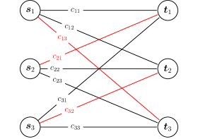
Figure 5.1: Bipartite graph formulation of a linear sum assignment problem (LSAP)

We introduce some terms to state the theorem below. A perfect matching is a subset of edges such that each vertex is incident to exactly one edge. The total weight of a perfect matching is the sum of weights of the edges in this matching. A perfect matching is called $(1+\epsilon)$-approximate for $\epsilon>0$ if its total weight is no larger than $(1+\epsilon)$ times the total weight of the optimal matching.

Theorem 5.1 (Gabow and Tarjan, (1989), Sharathkumar and Agarwal, (2012), Agarwal and Sharathkumar, (2014)).

Assume that points $\bm{s}_{i},\bm{t}_{j}\in{\mathbb{R}}^{d},~{}i,j\in\llbracket n\rrbracket$, have bounded integer coordinates, and that the squared distances $\lVert\bm{s}_{i}-\bm{t}_{j}\rVert^{2},~{}i,j\in\llbracket n\rrbracket$ are all bounded by some integer $N$. Then there exists an algorithm to find the optimal matching in $O(n^{5/2}\log(nN))$ time. Furthermore,

• if $d=2$, there exists an exact algorithm for computing the optimal matching in $O(n^{3/2+\delta}\log(N))$ time for any arbitrarily small constant $\delta>0$;

• if $d\geq 3$, there is an algorithm to compute a $(1+\epsilon)$-approximate perfect matching in
  $O(\epsilon^{-1}n^{3/2}\tau(n,\epsilon)\log^{4}(n/\epsilon)\log(\max c_{ij}/\min c_{ij}))$ time, where $\tau(n,\epsilon)$ depending on $n,\epsilon$ is small.

In the supplement we will describe the algorithm developed by Gabow and Tarjan, (1989) under the basic settings. It is essentially the combination of the Hungarian method (Kuhn, , 1955, 1956; Munkres, , 1957) and the algorithm of Hopcroft and Karp, (1973). We will ignore the details of the faster exact algorithm for $d=2$ by Sharathkumar and Agarwal, (2012) and the approximate algorithm for $d\geq 3$ by Agarwal and Sharathkumar, (2014); both algorithms improve the Gabow–Tarjan algorithm by exploiting the geometric structure of the weight matrix.

5.2 Eigenvalues and quadratic forms in normal variables

In Theorem 3.1, $\lambda_{k},~{}k\in{\mathbb{Z}}_{+}$, are non-zero eigenvalues (counted with multiplicity) of the integral equation

$${E}(d_{\bm{U}}(\bm{u},\bm{U})d_{\bm{V}}(\bm{v},\bm{V})\phi(\bm{U},\bm{V}))=\lambda\phi(\bm{u},\bm{v}).$$

Under the independence hypothesis $H_{0}$, the eigenvalues $\lambda_{k},~{}k\in{\mathbb{Z}}_{+}$, are given by all the products $\lambda_{1,j_{1}}\lambda_{2,j_{2}},~{}j_{1},j_{2}\in{\mathbb{Z}}_{+}$, where $\lambda_{1,j},~{}j\in{\mathbb{Z}}_{+}$, and $\lambda_{2,j},~{}j\in{\mathbb{Z}}_{+}$, are the non-zero eigenvalues of the integral equations

$${E}(d_{\bm{U}}(\bm{u},\bm{U})\phi_{1}(\bm{U}))=\lambda_{1}\phi_{1}(\bm{u})~{}~{}~{}\text{and}~{}~{}~{}{E}(d_{\bm{V}}(\bm{v},\bm{V})\phi_{2}(\bm{V}))=\lambda_{2}\phi_{2}(\bm{v}),$$

respectively (Nandy et al., , 2016, Lemma 4.2). The non-zero eigenvalues of integral equation ${E}(d_{\bm{U}}(\bm{u},\bm{U})\phi_{1}(\bm{U}))=\lambda_{1}\phi_{1}(\bm{u})$ with $\bm{U}\sim U_{p}$ are given by

$$-4/(\pi^{2}j^{2}),~{}~{}~{}{\rm for~{}all}~{}~{}j\in{\mathbb{Z}}_{+}~{}~{}{\rm when}~{}~{}p=1.$$

We are not aware of any closed form formulas for the eigenvalues when $p\geq 2$. However, in practice, the non-zero eigenvalues $\{\lambda_{1,j}\}_{j=1}^{\infty}$ can be numerically estimated by the non-zero eigenvalues of the matrix

$$(\mathbf{I}_{M}-\mathbf{J}_{M}/M)\mathbf{D}^{(M)}(\mathbf{I}_{M}-\mathbf{J}_{M}/M)/M,$$

denoted by $\lambda_{1,j}^{(M)},~{}j\in\llbracket M-1\rrbracket$, where $M:=M_{R}M_{S}$, $\mathbf{D}^{(M)}=[D_{jj^{\prime}}^{(M)}]$, $D_{jj^{\prime}}^{(M)}=\lVert\bm{u}_{j}^{(M)}-\bm{u}_{j^{\prime}}^{(M)}\rVert$ and $\bm{u}_{j}^{(M)},~{}j\in\llbracket M\rrbracket$, are points in the grid $\mathcal{G}^{p}_{0,M_{R},M_{S}}$. Here $\lambda_{1,j}^{(M)},~{}j\in\llbracket M-1\rrbracket$ are all negative (Lyons, , 2013, p. 3291). For $p=1$, we take $\lambda_{1,j}^{(M)}=-4/(\pi^{2}j^{2})$. We can obtain eigenvalues $\lambda_{2,j}^{(M)},~{}j\in\llbracket M-1\rrbracket$ based on the grid $\mathcal{G}^{q}_{0,M_{R},M_{S}}$ similarly. Then we sort the positive products $\lambda^{(M)}_{1,j_{1}}\lambda^{(M)}_{2,j_{2}},~{}j_{1},j_{2}\in\llbracket M-1\rrbracket$ into a descendingly ordered sequence $[\lambda^{(M)}_{k}]_{k=1}^{(M-1)^{2}}$, and have the following theorem.

Theorem 5.2.

Let $[\lambda_{k}]_{k=1}^{\infty}$ and $[\lambda^{(M)}_{k}]_{k=1}^{(M-1)^{2}}$ be eigenvalues as defined in Theorem 3.1 and above, respectively. Let $[\xi_{k}]_{k=1}^{\infty}$ be a sequence of independent standard Gaussian random variables. Then it holds for any pre-specified significance level $\alpha\in(0,1)$ that

$$Q_{1-\alpha}^{(M)}\to Q_{1-\alpha}$$

as $M_{R}\to\infty$ and $M_{S}\to\infty$, where $Q_{1-\alpha}^{(M)}$ and $Q_{1-\alpha}$ are the $(1-\alpha)$ quantiles of

$$\sum_{k=1}^{(M-1)^{2}}\lambda_{k}^{(M)}(\xi_{k}^{2}-1)~{}~{}~{}\text{and}~{}~{}~{}\sum_{k=1}^{\infty}\lambda_{k}(\xi_{k}^{2}-1),$$

respectively.

Consequently, we can approximate the $(1-\alpha)$ quantile of quadratic form $\sum_{k=1}^{\infty}\lambda_{k}(\xi_{k}^{2}-1)$ by estimating that of quadratic form $\sum_{k=1}^{(M-1)^{2}}\lambda_{k}^{(M)}(\xi_{k}^{2}-1)$ for a sufficiently large $M$. The latter is done by solving the inverse of the cumulative distribution function of quadratic form $\sum_{k=1}^{(M-1)^{2}}\lambda_{k}^{(M)}(\xi_{k}^{2}-1)$, which can be numerically evaluated using Farebrother, ’s (1984) algorithm or Imhof, ’s (1961) method.

6 Numerical studies

This section compares the performances of our tests using (i) the theoretical rejection threshold $Q_{1-\alpha}$ defined in (3.8) and computed using the approximation in Section 5.2, and (ii) a Monte Carlo simulation-based rejection threshold to the existing tests of independence that use (iii) distance covariance with marginal ranks (Lin, , 2017), and (iv) distance covariance (Székely and Rizzo, , 2013).

The test via distance covariance with marginal ranks proceeds as follows. Write $\bm{x}_{i}=(x_{i,1},...,x_{i,p})$ for $i\in\llbracket n\rrbracket$. Let $r_{i,k}$ be the rank of $x_{i,k}$ among $x_{1,k},x_{2,k},\dots,x_{n,k}$ for each $k\in\llbracket p\rrbracket$. The marginal rank (vector) of $\bm{x}_{i}$ is defined as $(r_{i,1},...,r_{i,p})$. The marginal rank (vector) of $\bm{y}_{i}$ is defined similarly. Then we run the permutation-based distance covariance test on the marginal ranks instead of the original data.

6.1 Simulation results

We first conduct Monte Carlo simulation experiments on the finite-sample performance of the proposed test from Section 3. We evaluate the empirical sizes and powers of the four competing tests stated above for both Gaussian and non-Gaussian distributions. The values reported below are based on $1,000$ simulations at the nominal significance level of $0.05$, with sample size $n\in\{216,432,864,1728\}$, dimensions $p=q\in\{2,3,5,{7}\}$, and correlation $\rho\in\{0,0.005,0.01,\dots,0.15\}$. More simulation studies on even higher dimensions of $p=q=10$ and 30 are presented in the supplement, Section C. For tests (iii) and (iv), we resample $n$ times in the permutation procedure.

Example 6.1.

The data $(X_{1},\ldots,X_{n})$ are independently drawn from $(\bm{X},\bm{Y})\in{\mathbb{R}}^{p+q}$, which follows a multivariate normal distribution with mean zero and covariance matrix $\mathbf{I}_{p+q}+\tau\mathbf{L}_{p+q;1,2}+\rho\mathbf{L}_{p+q;1,p+1}$ (where $\mathbf{L}_{d;i,j}:=\bm{e}_{d;i}\bm{e}_{d;j}^{\top}+\bm{e}_{d;j}\bm{e}_{d;i}^{\top}$ and $\bm{e}_{d;i}\in{\mathbb{R}}^{d}$ is the $i$-th standard basis vector in $d$-dimensional space, i.e., all entries are zero except for the one at the $i$-th position) with (a) $\tau=0$; (b) $\tau=0.5$; and (c) $\tau=0.9$.

Example 6.2.

The data $(X_{1},\ldots,X_{n})$ are independently drawn from $(\bm{X},\bm{Y})$, which is given by $X_{i}=Q_{t(1)}(\Phi(X_{i}^{*}))$, $i\in\llbracket p\rrbracket$ and $Y_{j}=Q_{t(1)}(\Phi(Y_{j}^{*}))$, $j\in\llbracket q\rrbracket$, where $Q_{t(1)}$ stands for the quantile function for Student’s $t$-distribution with $1$ degree of freedom (Cauchy distribution), and $(\bm{X}^{*},\bm{Y}^{*})$ are generated as in Example 6.1.

Table 6.1: Empirical sizes of the proposed test using theoretical (noted as Hallin(t)) and simulation-based (noted as Hallin(s)) rejection threshold, test via distance covariance with marginal ranks (noted as rdCov), and test via distance covariance (noted as dCov) in Example 6.1(a).

$(p,q)$	$n$	Hallin(t)	Hallin(s)	rdCov	dCov
$(2,2)$	$216$	0.040	0.043	0.043	0.045
$(2,2)$	$432$	0.037	0.047	0.048	0.050
$(2,2)$	$864$	0.045	0.045	0.050	0.048
$(2,2)$	$1728$	0.054	0.054	0.061	0.057
$(3,3)$	$216$	0.047	0.047	0.058	0.053
$(3,3)$	$432$	0.047	0.053	0.045	0.043
$(3,3)$	$864$	0.040	0.047	0.053	0.048
$(3,3)$	$1728$	0.049	0.049	0.043	0.050
$(5,5)$	$216$	0.040	0.043	0.040	0.048
$(5,5)$	$432$	0.033	0.043	0.048	0.043
$(5,5)$	$864$	0.047	0.050	0.040	0.048
$(5,5)$	$1728$	0.059	0.059	0.053	0.039
$(7,7)$	$216$	0.068	0.048	0.053	0.056
$(7,7)$	$432$	0.064	0.050	0.054	0.053
$(7,7)$	$864$	0.056	0.051	0.048	0.046
$(7,7)$	$1728$	0.052	0.054	0.048	0.052

In these two examples, the independence hypothesis holds when $\rho=0$. We first report the empirical sizes of all four considered tests, presented in Table 6.1. It can be observed that the proposed tests with either rejection threshold as well as their two competitors control the size effectively.

The empirical powers for Examples 6.1–6.2 are summarized in Figures 6.2–6.7. For the proposed test, we present results only for the theoretical rejection threshold as the results for the simulation-based threshold are similar and hence omitted.

Several facts are noteworthy. First, when the sample size is large and the dimension is relatively small, throughout all settings the performance of the proposed test is not much worse than the two competing ones. It should be highlighted that our method achieves this performance with smaller computational time, as shown in Figure 6.8 and also confirmed in our theoretical analysis of computational cost. Second, the proposed test beats the other two when the within-group correlation is high, i.e., as $\tau$ becomes larger from the setting (a) to (c), even when the dimension is high. Third, for heavy-tailed distributions, the tests via distance covariance with center-outward ranks and signs and marginal ranks perform better than the original distance covariance test. Lastly, compared to its competitors, the proposed test appears to be more sensitive to dimension. This is as expected.

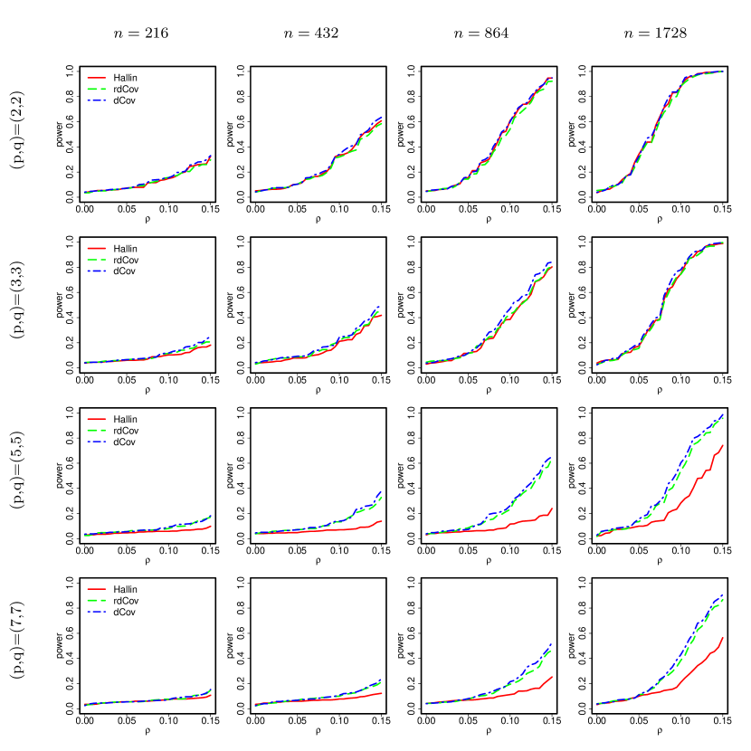
Figure 6.2: Empirical powers of the three competing tests in Example 6.1(a). The $y$-axis represents the power based on 1,000 replicates and the $x$-axis represents the level of a desired signal.

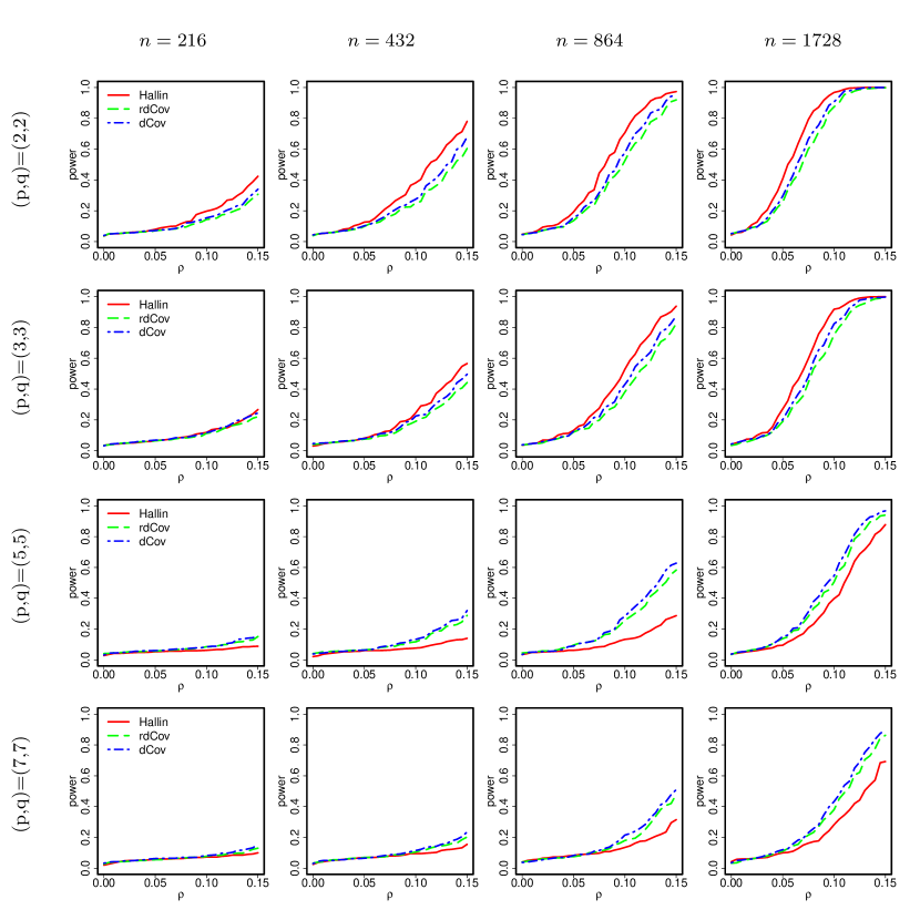
Figure 6.3: Empirical powers of the three competing tests in Example 6.1(b). The $y$-axis represents the power based on 1,000 replicates and the $x$-axis represents the level of a desired signal.

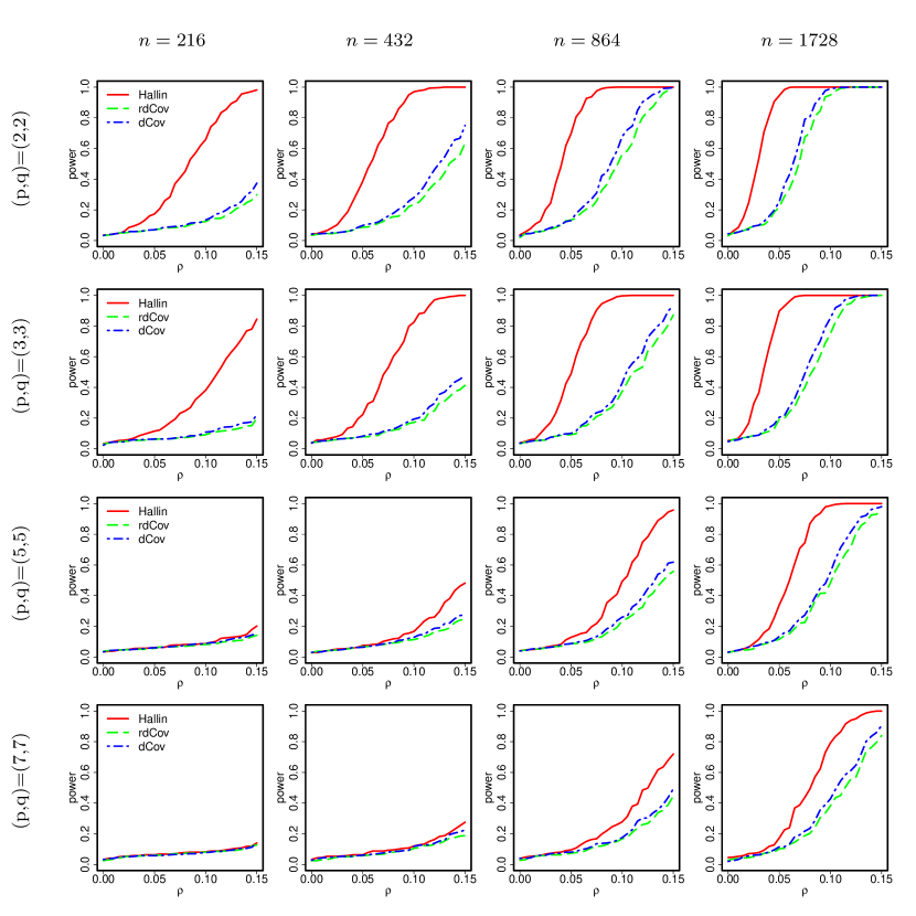
Figure 6.4: Empirical powers of the three competing tests in Example 6.1(c). The $y$-axis represents the power based on 1,000 replicates and the $x$-axis represents the level of a desired signal.

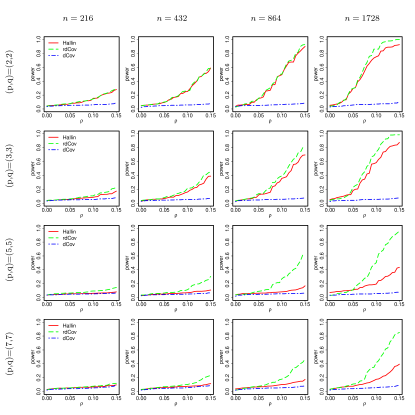
Figure 6.5: Empirical powers of the three competing tests in Example 6.2(a). The $y$-axis represents the power based on 1,000 replicates and the $x$-axis represents the level of a desired signal.

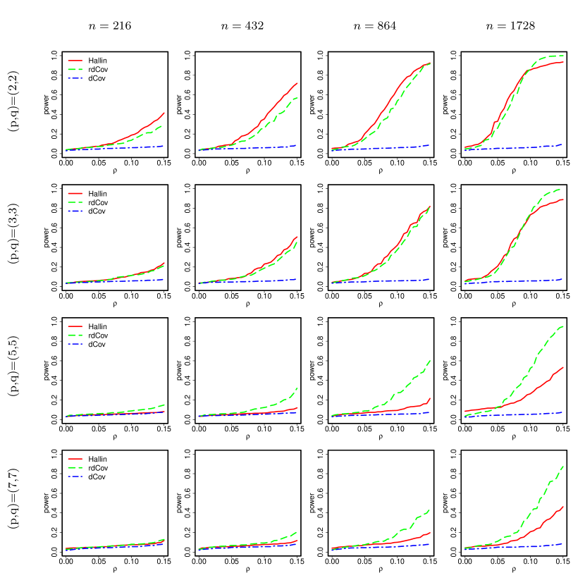
Figure 6.6: Empirical powers of the three competing tests in Example 6.2(b). The $y$-axis represents the power based on 1,000 replicates and the $x$-axis represents the level of a desired signal.

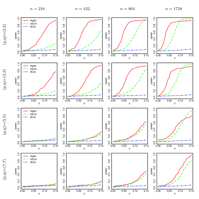
Figure 6.7: Empirical powers of the three competing tests in Example 6.2(c). The $y$-axis represents the power based on 1,000 replicates and the $x$-axis represents the level of a desired signal.

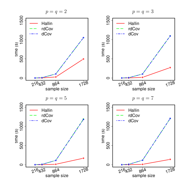
Figure 6.8: A comparison of computation time in Example 6.1(a) for the three tests. The $y$-axis represents the averaged computation elapsed time (in seconds) of 1,000 replicates of a single experiment and the $x$-axis represents the sample size. To compute the optimal matching, we used the algorithm in Gabow and Tarjan, (1989).

6.2 Real stock market data analysis

We analyze the monthly log returns of daily closing prices for stocks that are constantly in the Standard & Poor 100 (S&P 100) index during the time period 2003 to 2012. The data are from Yahoo! Finance (finance.yahoo.com), and the stocks are classified into 10 sectors by Global Industry Classification Standard (GICS). Stock market data tend to be heavy-tailed with many outliers, and monthly log returns may reasonably be modeled as independent and identically distributed random variables. The time period we analyzed includes some well known turbulent stretches like the 2007-08 financial crisis, which, however, could be either explained using heavy-tailed (e.g., elliptical or stable) distribution models or captured as outliers.

In this section we limit our scope and focus on detecting between-group dependence between two sectors in S& P 100 that contain a rather small number of stocks: (1) Telecommunication, including stocks “AT&T Inc [T]” and “Verizon Communications [VZ]”; and (2) Materials, including stocks “Du Pont (E.I.) [DD]”, “Dow Chemical [DOW]”, “Freeport-McMoran Cp & Gld [FCX]”, and “Monsanto Co. [MON]”. We then consider detection of possible dependence between the Telecommunication sector and any two stocks in the Materials sector.

To this end, we apply the three considered tests to the monthly log returns of (T,VZ) coupled with either (DD,DOW), or (DD,FCX), or (DD,MON), or (DOW,FCX), or (DOW,MON), or (FCX,MON). The p-values for these three tests are reported in Table 6.2. There, one observes that using the proposed test yields uniformly the strongest evidence to conclude the existence of dependence between (T,VZ) and any two stocks in the Materials sector.

Table 6.2: P-values based on the proposed test as well as two competing tests for the dataset of US stock closing prices between 2003 and 2012.

		(DD,DOW)	(DD,FCX)	(DD,MON)	(DOW,FCX)	(DOW,MON)	(FCX,MON)
Hallin	(T, VZ)	0.001	0.005	0.002	0.004	0.001	0.065
rdCov	(T, VZ)	0.002	0.013	0.005	0.009	0.002	0.070
dCov	(T, VZ)	0.002	0.018	0.003	0.012	0.002	0.101

Appendix A Proofs

Further concepts concerning U-statistics are needed. For any symmetric kernel $h$, any integer $\ell\in\llbracket m\rrbracket$, and any probability measure ${P}_{\bm{X}}$, we remind the definition of

$$h_{\ell}(\bm{x}_{1}\ldots,\bm{x}_{\ell};{P}_{\bm{X}}) :={E}h(\bm{x}_{1}\ldots,\bm{x}_{\ell},\bm{X}_{\ell+1},\ldots,\bm{X}_{m}),$$

and write

$$\widetilde{h}_{\ell}(\bm{x}_{1},\ldots,\bm{x}_{\ell};{P}_{\bm{X}}) :=h_{\ell}(\bm{x}_{1},\ldots,\bm{x}_{\ell};{P}_{\bm{X}})-{E}h-\sum_{k=1}^{\ell-1}\sum_{1\leq i_{1}<\cdots<i_{k}\leq\ell}\widetilde{h}_{k}(\bm{x}_{i_{1}},\ldots,\bm{x}_{i_{k}};{P}_{\bm{X}}),$$ (A.1)

where $\bm{X}_{1},\ldots,\bm{X}_{m}$ are $m$ independent random variables with law ${P}_{\bm{X}}$ and ${E}h:={E}h(\bm{X}_{1},\ldots,\bm{X}_{m})$. We also have

$$\binom{n}{m}^{-1}\sum_{1\leq i_{1}<i_{2}<\cdots<i_{m}\leq n}h\Big{(}\bm{X}^{\prime}_{i_{1}},\ldots,\bm{X}^{\prime}_{i_{m}}\Big{)}$$

$$=\; {E}h+\sum_{\ell=1}^{m}\binom{m}{\ell}\binom{n}{\ell}^{-1}\sum_{1\leq i_{1}<i_{2}<\cdots<i_{\ell}\leq n}\widetilde{h}_{\ell}\Big{(}\bm{X}^{\prime}_{i_{1}},\ldots,\bm{X}^{\prime}_{i_{\ell}};{P}_{\bm{X}}\Big{)},$$ (A.2)

for any (possibly dependent) random variables $\bm{X}^{\prime}_{1},\dots,\bm{X}^{\prime}_{n}$. This is the Hoeffding decomposition with respect to ${P}_{\bm{X}}$.

Additional notation.

Let $(n)_{r}$ denote $n!/(n-r)!$. The cardinality of a set $\mathcal{S}$ is written $\mathrm{card}(\mathcal{S})$. For a multiset $\mathcal{M}=\{x_{1},\dots,x_{n}\}$ and $r\in\llbracket n\rrbracket$, an $r$-permutation of $\mathcal{M}$ is a sequence $[x_{\sigma(i)}]_{i=1}^{r}$, where $\sigma$ is a bijection from $\llbracket n\rrbracket$ to itself. For $r\in\llbracket n\rrbracket$, let $I^{n}_{r}$ denote the family of all $(n)_{r}$ possible $r$-permutations of set $\llbracket n\rrbracket$. For $x\in{\mathbb{R}}$, let $x_{+}=\max\{x,0\}$ denote the positive part of $x$. Let $\bm{x}\circ\bm{y}$ and $\bm{x}\cdot\bm{y}$ denote the Hadamard product and dot product of two vectors $\bm{x},\bm{y}\in{\mathbb{R}}^{d}$, respectively. We use $\stackrel{{\scriptstyle\sf p}}{{\longrightarrow}}$ to denote convergence in probability. We use $\mathsf{i}$ to represent the imaginary unit.

A.1 Proofs for Section 2 of the main paper

A.1.1 Proof of Proposition 2.2

Proof of Proposition 2.2.

We first prove the case $n_{0}=0$ and then generalize to $n_{0}>0$. For simpler presentation, let $\lambda_{n_{0},n_{R},{n_{S}}}$ denote the uniform measure (distribution) on the augmented grid $\mathcal{G}^{d}_{n_{0},n_{R},{n_{S}}}$, let $\mu_{n_{R}}$ denote the uniform measure on the points $\{\frac{j}{n_{R}+1}:j\in\llbracket n_{R}\rrbracket\}$, and let $\nu_{{n_{S}}}$ denote the uniform measure on the points $\{\bm{r}_{k}:k\in\llbracket n_{S}\rrbracket\}$. Furthermore, let $\mu$ denote the uniform measure on $[0,1)$, and let $\nu$ denote the uniform measure over the unit sphere $\mathcal{S}_{d-1}$.

If $n_{0}=0$, then $\lambda_{n_{0},n_{R},{n_{S}}}$ is the product measure of $\mu_{n_{R}}$ (for the radius) and $\nu_{\bm{n_{S}}}$ (for the unit sphere). By assumption, $\nu_{{n_{S}}}$ weakly converges to $\nu$ as $n_{S}\to\infty$. Moreover, $\mu_{n_{R}}$ weakly converges to $\mu$ as $n_{R}\to\infty$ by the following argument:

$$\mu_{n_{R}}\Big{(}(0,x]\Big{)}=\frac{\lfloor n_{R}x\rfloor}{n_{R}}\to x=\mu\Big{(}(0,x]\Big{)},~{}~{}~{}\text{for}~{}x\in(0,1),$$

as $n_{R}\to\infty$. Combining these facts, and applying Theorem 2.8 in Billingsley, (1999) to the separable space $\mathbb{S}_{d}$, we deduce that $\lambda_{n_{0},n_{R},{n_{S}}}$, the product measure of $\mu_{n_{R}}$ and $\nu_{{n_{S}}}$, weakly converges to $\mu\times\nu=U_{d}$ as $n_{R},n_{S}\to\infty$.

If $n_{0}>0$, we compare the uniform measure on the augmented grid $\mathcal{G}^{d}_{0,n_{R},{n_{S}}}$ (denoted by $\lambda_{0,n_{R},{n_{S}}}$) and that on $\mathcal{G}^{d}_{n_{0},n_{R},{n_{S}}}$. For any $U_{d}$-continuity set $D\subseteq\mathbb{S}_{d}$, we obtain

$$\lambda_{0,n_{R},{n_{S}}}(D)=\frac{\mathrm{card}(D\cap\mathcal{G}^{d}_{0,n_{R},{n_{S}}})}{n-n_{0}}~{}~{}~{}\text{and}~{}~{}~{}\lambda_{n_{0},n_{R},{n_{S}}}(D)=\frac{\mathrm{card}(D\cap\mathcal{G}^{d}_{0,n_{R},{n_{S}}})+n_{0}\mathds{1}(\bm{0}\in D)}{n}.$$

Therefore,

$$\lvert\lambda_{0,n_{R},{n_{S}}}(D)-\lambda_{n_{0},n_{R},{n_{S}}}(D)\rvert\leq\; \Big{(}\frac{1}{n-n_{0}}-\frac{1}{n}\Big{)}\mathrm{card}(D\cap\mathcal{G}^{d}_{0,n_{R},{n_{S}}})+\frac{n_{0}}{n}$$

$$\leq\; \Big{(}\frac{1}{n-n_{0}}-\frac{1}{n}\Big{)}(n-n_{0})+\frac{n_{0}}{n}=\frac{2n_{0}}{n}\to 0,$$ (A.3)

where the last step follows by noticing

$$\frac{n_{0}}{n}<\frac{\min\{n_{R},n_{S}\}}{n}\leq\frac{n_{S}}{n_{R}n_{S}+n_{0}}\leq\frac{1}{n_{R}}\to 0$$

as $n_{R}\to\infty$. We have proven in the case $n_{0}=0$ that $\lambda_{0,n_{R},{n_{S}}}$ weakly converges to $U_{d}$ and then $\lambda_{0,n_{R},{n_{S}}}(D)\to U_{d}(D)$. This, together with (A.3), proves that $\lambda_{n_{0},n_{R},{n_{S}}}(D)\to U_{d}(D)$ for any $U_{d}$-continuity Borel set $D\subseteq\mathbb{S}_{d}$, and equivalently, $\lambda_{n_{0},n_{R},{n_{S}}}$ weakly converges to $U_{d}$ as $n_{R},n_{S}\to\infty$. ∎

A.2 Proofs for Section 3 of the main paper

A.2.1 Proof of Proposition 3.1

Proof.

The equivalence of these three versions of the sample distance covariance is well known; we include a proof for completeness but claim no originality here.

The sample distance covariance defined in Székely and Rizzo, (2013) and Székely and Rizzo, (2014) can be described as follows. First define

$$a_{i,j} :=\lVert\bm{X}_{i}-\bm{X}_{j}\rVert,~{}~{}~{}a_{i,+}:=\sum_{\ell=1}^{n}a_{i,\ell},~{}~{}~{}a_{+,j}:=\sum_{k=1}^{n}a_{k,j},~{}~{}~{}a_{+,+}:=\sum_{k,\ell=1}^{n}a_{k,\ell},$$

$$A^{*}_{i,j} :=\begin{cases}a_{i,j}-\frac{1}{n-1}a_{i,+}-\frac{1}{n-1}a_{+,j}+\frac{1}{n(n-1)}a_{+,+},&\text{if }i\neq j,\\ \frac{1}{n-1}a_{i,+}-\frac{1}{n(n-1)}a_{+,+},&\text{if }i=j,\end{cases}$$

$$\widetilde{A}_{i,j} :=\begin{cases}a_{i,j}-\frac{1}{n-2}a_{i,+}-\frac{1}{n-2}a_{+,j}+\frac{1}{(n-1)(n-2)}a_{+,+},&\text{if }i\neq j,\\ 0,&\text{if }i=j,\end{cases}$$

Similarly, we introduce the distances $b_{i,j}:=\lVert\bm{Y}_{i}-\bm{Y}_{j}\rVert$, and define the sums $b_{i,+},b_{+,j},b_{+,+}$, and corresponding $B^{*}_{i,j}$, $\widetilde{B}_{i,j}$ in analogy to the quantities for the $\bm{X}_{i}$. Then the sample distance covariance from Definition 1 in Székely and Rizzo, (2013) is

$$\mathrm{dCov}^{2}_{n}\Big{(}[\bm{X}_{i}]_{i=1}^{n},[\bm{Y}_{i}]_{i=1}^{n}\Big{)}:=\frac{1}{n(n-3)}\Big{\{}\sum_{i,j=1}^{n}A^{*}_{i,j}B^{*}_{i,j}-\frac{n}{n-2}\sum_{i=1}^{n}A^{*}_{i,i}B^{*}_{i,i}\Big{\}},$$ (A.4)

and the sample distance covariance from Equation (3.2) in Székely and Rizzo, (2014) is

$$\mathrm{dCov}^{2}_{n}\Big{(}[\bm{X}_{i}]_{i=1}^{n},[\bm{Y}_{i}]_{i=1}^{n}\Big{)}:=\frac{1}{n(n-3)}\sum_{i\neq j}\widetilde{A}_{i,j}\widetilde{B}_{i,j}.$$ (A.5)

We first prove the equivalence between (A.4) and (A.5). Lemma 3.1 in Huo and Székely, (2016) gives that the right-hand side of (A.5) equals to

$$\frac{1}{n(n-3)}\sum_{i\neq j}a_{i,j}b_{i,j}-\frac{2}{n(n-2)(n-3)}\sum_{i=1}^{n}a_{i,+}b_{i,+}+\frac{a_{+,+}b_{+,+}}{n(n-1)(n-2)(n-3)}.$$ (A.6)

It remains to prove that the right-hand side of (A.4) equals to (A.6) as well, which can be established by straightforward calculation following the proof of Lemma 3.1 in Huo and Székely, (2016). First, one can verify the following equalities:

$$a_{i,j}=a_{j,i},~{}~{}~{}a_{i,i}=0,~{}~{}~{}a_{i,+}=a_{+,i},~{}~{}~{} b_{i,j}=b_{j,i},~{}~{}~{}b_{i,i}=0,~{}~{}~{}b_{i,+}=b_{+,i},$$ (A.7)

$$\sum_{i\neq j}a_{i,j}=a_{+,+},~{}~{}~{} \sum_{i\neq j}b_{i,j}=b_{+,+},$$ (A.8)

$$\sum_{i\neq j}a_{i,+}=\sum_{i\neq j}a_{+,j}=(n-1)a_{+,+},~{}~{}~{} \sum_{i\neq j}b_{i,+}=\sum_{i\neq j}b_{+,j}=(n-1)b_{+,+},$$ (A.9)

$$\sum_{i\neq j}a_{i,j}b_{i,+}=\sum_{i\neq j}a_{i,j}b_{+,j}=\sum_{i=1}^{n}a_{i,+}b_{i,+},~{}~{}~{} \sum_{i\neq j}a_{i,+}b_{i,j}=\sum_{i\neq j}a_{+,j}b_{i,j}=\sum_{i=1}^{n}a_{i,+}b_{i,+},$$ (A.10)

$$\sum_{i\neq j}a_{i,+}b_{+,j}=a_{+,+}b_{+,+}-\sum_{i=1}^{n}a_{i,+}b_{i,+},~{}~{}~{} \sum_{i\neq j}a_{+,j}b_{i,+}=a_{+,+}b_{+,+}-\sum_{i=1}^{n}a_{i,+}b_{i,+}.$$ (A.11)

Next, we may simplify the right-hand side of (A.4). We have

$$\frac{1}{n(n-3)}\Big{\{}\sum_{i,j=1}^{n}A^{*}_{i,j}B^{*}_{i,j}-\frac{n}{n-2}\sum_{i=1}^{n}A^{*}_{i,i}B^{*}_{i,i}\Big{\}}=\frac{1}{n(n-3)}\Big{\{}\sum_{i\neq j}A^{*}_{i,j}B^{*}_{i,j}-\frac{2}{n-2}\sum_{i=1}^{n}A^{*}_{i,i}B^{*}_{i,i}\Big{\}},$$

where

$$\sum_{i\neq j}A^{*}_{i,j}B^{*}_{i,j}\; =\sum_{i\neq j}\Big{(}a_{i,j}-\frac{a_{i,+}}{n-1}-\frac{a_{+,j}}{n-1}+\frac{a_{+,+}}{n(n-1)}\Big{)}\Big{(}b_{i,j}-\frac{b_{i,+}}{n-1}-\frac{b_{+,j}}{n-1}+\frac{b_{+,+}}{n(n-1)}\Big{)}$$

$$=\sum_{i\neq j}\Big{(}a_{i,j}b_{i,j}-\frac{a_{i,j}(b_{i,+}+b_{+,j})+(a_{i,+}+a_{+,j})b_{i,j}}{n-1}+\frac{(a_{i,+}+a_{+,j})(b_{i,+}+b_{+,j})}{(n-1)^{2}}$$

$$\quad+\frac{a_{i,j}b_{+,+}+a_{+,+}b_{i,j}}{n(n-1)}-\frac{(a_{i,+}+a_{+,j})b_{+,+}+a_{+,+}(b_{i,+}+b_{+,j})}{n(n-1)^{2}}+\frac{a_{+,+}b_{+,+}}{n^{2}(n-1)^{2}}\Big{)},\!\!\!$$ (A.12)

$$\sum_{i=1}^{n}A^{*}_{i,i}B^{*}_{i,i}\; =\sum_{i=1}^{n}\Big{(}\frac{a_{i,+}}{n-1}-\frac{a_{+,+}}{n(n-1)}\Big{)}\Big{(}\frac{b_{i,+}}{n-1}-\frac{b_{+,+}}{n(n-1)}\Big{)}$$

$$=\frac{1}{(n-1)^{2}}\sum_{i=1}^{n}\Big{(}a_{i,+}b_{i,+}-\frac{a_{i,+}b_{+,+}+a_{+,+}b_{i,+}}{n}+\frac{a_{+,+}b_{+,+}}{n^{2}}\Big{)}.$$ (A.13)

Furthermore, we have

$$\sum_{i\neq j}\frac{a_{i,j}(b_{i,+}+b_{+,j})+(a_{i,+}+a_{+,j})b_{i,j}}{n-1}\xlongequal{\eqref{eq:huoeq3}}\frac{4}{n-1}\sum_{i=1}^{n}a_{i,+}b_{i,+}$$

$$\sum_{i\neq j}\frac{(a_{i,+}+a_{+,j})(b_{i,+}+b_{+,j})}{(n-1)^{2}}\xlongequal{\eqref{eq:huoeq5}}\frac{1}{(n-1)^{2}}\Big{\{}2(n-2)\sum_{i=1}^{n}a_{i,+}b_{i,+}+2a_{+,+}b_{+,+}\Big{\}},$$

$$\sum_{i\neq j}\frac{a_{i,j}b_{+,+}+a_{+,+}b_{i,j}}{n(n-1)}\xlongequal{\eqref{eq:huoeq1.5}}\frac{2a_{+,+}b_{+,+}}{n(n-1)},$$

$$\sum_{i\neq j}\frac{(a_{i,+}+a_{+,j})b_{+,+}+a_{+,+}(b_{i,+}+b_{+,j})}{n(n-1)^{2}}\xlongequal{\eqref{eq:huoeq2}}\frac{4a_{+,+}b_{+,+}}{n(n-1)},$$

$$\sum_{i\neq j}\frac{a_{+,+}b_{+,+}}{n^{2}(n-1)^{2}}=\frac{a_{+,+}b_{+,+}}{n(n-1)},$$

and $$\sum_{i=1}^{n}\frac{a_{i,+}b_{+,+}+a_{+,+}b_{i,+}}{n}=\frac{2a_{+,+}b_{+,+}}{n},~{}~{}~{}\sum_{i=1}^{n}\frac{a_{+,+}b_{+,+}}{n^{2}}=\frac{a_{+,+}b_{+,+}}{n}.$$

Plugging all these equalities above into (A.12) and (A.13) completes the proof.

The equivalence between (A.5) and (3.3) is an immediate consequence of Lemma 1 in Yao et al., 2018b , which shows that (A.5) is equivalent to

$$\mathrm{dCov}^{2}_{n}\Big{(}[\bm{X}_{i}]_{i=1}^{n},[\bm{Y}_{i}]_{i=1}^{n}\Big{)}:=\binom{n}{4}^{-1}\sum_{1\leq i_{1}<\dots<i_{4}\leq n}K^{\prime}\Big{(}(\bm{X}_{i_{1}},\bm{Y}_{i_{1}}),\dots,(\bm{X}_{i_{4}},\bm{Y}_{i_{4}})\Big{)},$$ (A.14)

where

$$K^{\prime}\Big{(}(\bm{x}_{1},\bm{y}_{1}),\dots,(\bm{x}_{4},\bm{y}_{4})\Big{)}$$

$$:=\; \frac{1}{4!}\sum_{[i_{1},\dots,i_{4}]\in\mathscr{P}(\llbracket 4\rrbracket)}\lVert\bm{x}_{i_{1}}-\bm{x}_{i_{2}}\rVert\Big{(}\lVert\bm{y}_{i_{1}}-\bm{y}_{i_{2}}\rVert+\lVert\bm{y}_{i_{3}}-\bm{y}_{i_{4}}\rVert-2\lVert\bm{y}_{i_{1}}-\bm{y}_{i_{3}}\rVert\Big{)}.$$

By expanding the above summation, one obtains that (A.14) is equivalent to

$$\mathrm{dCov}^{2}_{n}\Big{(}[\bm{X}_{i}]_{i=1}^{n},[\bm{Y}_{i}]_{i=1}^{n}\Big{)}:=\binom{n}{4}^{-1}\sum_{1\leq i_{1}<\dots<i_{4}\leq n}K^{\prime\prime}\Big{(}(\bm{X}_{i_{1}},\bm{Y}_{i_{1}}),\dots,(\bm{X}_{i_{4}},\bm{Y}_{i_{4}})\Big{)},$$ (A.15)

where

$$K^{\prime\prime}\Big{(}(\bm{x}_{1},\bm{y}_{1}),\dots,(\bm{x}_{4},\bm{y}_{4})\Big{)}$$

$$:=\; \frac{1}{4!}\sum_{[i_{1},\dots,i_{4}]\in\mathscr{P}(\llbracket 4\rrbracket)}\lVert\bm{x}_{i_{1}}-\bm{x}_{i_{2}}\rVert\Big{(}\lVert\bm{y}_{i_{1}}-\bm{y}_{i_{2}}\rVert+\lVert\bm{y}_{i_{3}}-\bm{y}_{i_{4}}\rVert-\lVert\bm{y}_{i_{1}}-\bm{y}_{i_{3}}\rVert-\lVert\bm{y}_{i_{2}}-\bm{y}_{i_{4}}\rVert\Big{)}.$$

Next, by expanding the summation again, we have (A.15) is equivalent to (3.3).

Definition 5.3 (U-statistic) in Jakobsen, (2017) can be written as

$$\mathrm{dCov}^{2}_{n}\Big{(}[\bm{X}_{i}]_{i=1}^{n},[\bm{Y}_{i}]_{i=1}^{n}\Big{)}:=\binom{n}{6}^{-1}\sum_{1\leq i_{1}<\dots<i_{6}\leq n}K^{*}\Big{(}(\bm{X}_{i_{1}},\bm{Y}_{i_{1}}),\dots,(\bm{X}_{i_{6}},\bm{Y}_{i_{6}})\Big{)},$$ (A.16)

where

$$K^{*}\Big{(}(\bm{x}_{1},\bm{y}_{1}),\dots,(\bm{x}_{6},\bm{y}_{6})\Big{)} :=\frac{1}{6!}\sum_{[i_{1},\dots,i_{6}]\in\mathscr{P}(\llbracket 6\rrbracket)}s(\bm{x}_{i_{1}},\bm{x}_{i_{2}},\bm{x}_{i_{3}},\bm{x}_{i_{4}})s(\bm{y}_{i_{1}},\bm{y}_{i_{2}},\bm{y}_{i_{5}},\bm{y}_{i_{6}}),$$

$$\text{and recall}~{}~{}~{}s(\bm{t}_{1},\bm{t}_{2},\bm{t}_{3},\bm{t}_{4}) :=\lVert\bm{t}_{1}-\bm{t}_{2}\rVert+\lVert\bm{t}_{3}-\bm{t}_{4}\rVert-\lVert\bm{t}_{1}-\bm{t}_{3}\rVert-\lVert\bm{t}_{2}-\bm{t}_{4}\rVert.$$

The equivalence between (A.16) and (3.3) can be verified by expanding the summation as well. ∎

A.2.2 Proof of Theorem 3.1

Proof of Theorem 3.1.

This theorem is a corollary of Theorem 4.2, which we prove in Section A.3.2. In our context, $p_{1}=p$, $p_{2}=q$, $m=4$, and $h$ is the kernel $K$ defined in (3.4). The multisets $\{\bm{z}^{(n)}_{1;j},j\in\llbracket n\rrbracket\}$ and $\{\bm{z}^{(n)}_{2;j},j\in\llbracket n\rrbracket\}$ are taken to be $\{\bm{u}^{(n)}_{j},j\in\llbracket n\rrbracket\}:=\mathcal{G}^{p}_{n_{0},n_{R},\bm{n_{S}}}$ and $\{\bm{v}^{(n)}_{j},j\in\llbracket n\rrbracket\}:=\mathcal{G}^{q}_{n_{0},n_{R},\bm{n_{S}}}$, respectively. Accordingly, $\bm{Z}^{(n)}_{1}$ follows the uniform discrete distribution over $\mathcal{G}^{p}_{n_{0},n_{R},\bm{n_{S}}}$, denoted by $\bm{U}^{(n)}$, and $\bm{Z}^{(n)}_{2}$ has a uniform discrete distribution over $\mathcal{G}^{q}_{n_{0},n_{R},\bm{n_{S}}}$, denoted by $\bm{V}^{(n)}$. The functions $g^{(n)}_{1}$, $g_{1}$, $g^{(n)}_{2}$, and $g_{2}$ can be chosen as $-d_{\bm{U}^{(n)}}$, $-d_{\bm{U}}$, $-d_{\bm{V}^{(n)}}$, and $-d_{\bm{V}}$, defined in the manner of (3.2), respectively. Recall that

$$d_{\bm{U}^{(n)}}(\bm{u},\bm{u}^{\prime}) :=\lVert\bm{u}-\bm{u}^{\prime}\rVert-{E}\lVert\bm{u}-\bm{U}^{(n)}_{2}\rVert-{E}\lVert\bm{U}^{(n)}_{1}-\bm{u}^{\prime}\rVert+{E}\lVert\bm{U}^{(n)}_{1}-\bm{U}^{(n)}_{2}\rVert,$$

$$\text{and}~{}~{}~{}d_{\bm{U}}(\bm{u},\bm{u}^{\prime}) :=\lVert\bm{u}-\bm{u}^{\prime}\rVert-{E}\lVert\bm{u}-\bm{U}_{2}\rVert-{E}\lVert\bm{U}_{1}-\bm{u}^{\prime}\rVert+{E}\lVert\bm{U}_{1}-\bm{U}_{2}\rVert,$$ (A.17)

with their analogues $d_{\bm{V}^{(n)}}(\bm{v},\bm{v}^{\prime})$ and $d_{\bm{V}}(\bm{v},\bm{v}^{\prime})$. Here $\bm{U}^{(n)}_{1}$ and $\bm{U}^{(n)}_{2}$ are independent with law ${P}_{\bm{U}^{(n)}}$, and $\bm{U}_{1}$ and $\bm{U}_{2}$ are independent with law ${P}_{\bm{U}}$.

We verify the conditions in Theorem 4.2 as follows. Proposition 2.2 shows that $\bm{U}^{(n)}$ and $\bm{V}^{(n)}$ converge in distribution to $\bm{U}$ and $\bm{V}$, respectively. We also have that (I) the kernel $K$ is symmetric and continuous on $\overline{\mathbb{S}}_{p}\times\overline{\mathbb{S}}_{q}$, and thus $\lVert K\rVert_{\infty}<\infty$; (II) $K_{1}(\bm{w};{P}_{\bm{U}^{(n)}}\times{P}_{\bm{V}^{(n)}})=0$; (III)

$$6K_{2}\Big{(}\bm{w},\bm{w}^{\prime};{P}_{\bm{U}^{(n)}}\times{P}_{\bm{V}^{(n)}}\Big{)} =\Big{(}-d_{\bm{U}^{(n)}}(\bm{u},\bm{u}^{\prime})\Big{)}\Big{(}-d_{\bm{V}^{(n)}}(\bm{v},\bm{v}^{\prime})\Big{)},$$

$$\text{and}~{}~{}~{}6K_{2}\Big{(}\bm{w},\bm{w}^{\prime};{P}_{\bm{U}}\times{P}_{\bm{V}}\Big{)} =\Big{(}-d_{\bm{U}}(\bm{u},\bm{u}^{\prime})\Big{)}\Big{(}-d_{\bm{V}}(\bm{v},\bm{v}^{\prime})\Big{)},$$

by Yao et al., 2018a (, Sec. 1.1).

Next we verify Assumptions (i)–(vi) for $-d_{\bm{U}^{(n)}}(\bm{u},\bm{u}^{\prime})$ and $-d_{\bm{U}}(\bm{u},\bm{u}^{\prime})$. It can be easily seen that $-d_{\bm{U}^{(n)}}(\bm{u},\bm{u}^{\prime})$ is symmetric (Assumption (i)), and has ${E}[-d_{\bm{U}^{(n)}}(\bm{u},\bm{U}^{(n)})]=0$ (Assumption (iv)) and ${E}[\{d_{\bm{U}^{(n)}}(\bm{U}^{(n)},\bm{U}^{(n)}_{*})\}^{2}]\in(0,+\infty)$ (Assumption (v)) by Székely et al., (2007, Theorem 4(i)). Lyons, (2013, p. 3291) has proved that functions $-d_{\bm{U}^{(n)}}(\bm{u},\bm{u}^{\prime})$ are non-negative definite (Assumption (iii)). We have $-d_{\bm{U}^{(n)}}(\bm{u},\bm{u}^{\prime})$ is equicontinuous (Assumption (ii)) since

$$\lvert-d_{\bm{U}^{(n)}}(\bm{u},\bm{u}^{\prime})-(-d_{\bm{U}^{(n)}}(\bm{u},\bm{u}^{\prime\prime}))\rvert \;=\Big{\lvert}\lVert\bm{u}-\bm{u}^{\prime}\rVert-\lVert\bm{u}-\bm{u}^{\prime\prime}\rVert-{E}\Big{[}\lVert\bm{U}^{(n)}-\bm{u}^{\prime}\rVert-\lVert\bm{U}^{(n)}-\bm{u}^{\prime\prime}\rVert\Big{]}\Big{\rvert}$$

$$\;\leq 2\lVert\bm{u}^{\prime}-\bm{u}^{\prime\prime}\rVert,$$

and moreover, $\lvert-d_{\bm{U}^{(n)}}(\bm{u},\bm{u}^{\prime})-(-d_{\bm{U}^{(n)}}(\bm{u}^{\prime\prime\prime},\bm{u}^{\prime\prime}))\rvert\leq 2\lVert\bm{u}-\bm{u}^{\prime\prime\prime}\rVert+2\lVert\bm{u}^{\prime}-\bm{u}^{\prime\prime}\rVert.$ It remains to prove that $-d_{\bm{U}^{(n)}}(\bm{u},\bm{u}^{\prime})$ converges uniformly to $-d_{\bm{U}}(\bm{u},\bm{u}^{\prime})$ (Assumption (vi)). Using the portmanteau Lemma (van der Vaart, , 1998, Lemma 2.2) and Proposition 2.2, we have for all $\bm{u},\bm{u}^{\prime}\in\overline{\mathbb{S}}_{p}$,

$${E}\lVert\bm{u}-\bm{U}^{(n)}_{*}\rVert\to{E}\lVert\bm{u}-\bm{U}_{*}\rVert,~{}~{}~{}{E}\lVert\bm{U}^{(n)}-\bm{u}^{\prime}\rVert\to{E}\lVert\bm{U}-\bm{u}^{\prime}\rVert,$$

$$~{}~{}~{}\text{and}~{}~{}~{}{E}\lVert\bm{U}^{(n)}-\bm{U}^{(n)}_{*}\rVert\to{E}\lVert\bm{U}-\bm{U}_{*}\rVert,$$

and thus $-d_{\bm{U}^{(n)}}(\bm{u},\bm{u}^{\prime})$ converges pointwisely to $-d_{\bm{U}}(\bm{u},\bm{u}^{\prime})$. Then the uniform convergence follows from the equicontinuity of $-d_{\bm{U}^{(n)}}(\bm{u},\bm{u}^{\prime})$ (Rudin, , 1976, Exercise 7.16). Assumptions (i)–(vi) can be similarly verified for $-d_{\bm{V}^{(n)}}(\bm{v},\bm{v}^{\prime})$ and $-d_{\bm{V}}(\bm{v},\bm{v}^{\prime})$ as well.

Lastly, using Proposition 2.4, $[\mathbf{F}^{(n)}_{\bm{X},\pm}(\bm{X}_{i})]_{i=1}^{n}$ and $[\mathbf{F}^{(n)}_{\bm{Y},\pm}(\bm{Y}_{i})]_{i=1}^{n}$ are uniformly distributed on $\mathscr{P}(\mathcal{G}^{p}_{n_{0},n_{R},\bm{n_{S}}})$ and $\mathscr{P}(\mathcal{G}^{q}_{n_{0},n_{R},\bm{n_{S}}})$, respectively. In addition, under $H_{0}$, $[\mathbf{F}^{(n)}_{\bm{X},\pm}(\bm{X}_{i})]_{i=1}^{n}$ and $[\mathbf{F}^{(n)}_{\bm{Y},\pm}(\bm{Y}_{i})]_{i=1}^{n}$ are independent. Hence our statistic is distributed as

$$\widehat{M}_{n}=n\cdot\binom{n}{4}^{-1}\sum_{1\leq j_{1}<\cdots<j_{4}\leq n}K\Big{(}(\bm{u}^{(n)}_{\pi^{\prime}_{j_{1}}},\bm{v}^{(n)}_{\pi^{\prime\prime}_{j_{1}}}),\ldots,(\bm{u}^{(n)}_{\pi^{\prime}_{j_{4}}},\bm{v}^{(n)}_{\pi^{\prime\prime}_{j_{4}}})\Big{)},$$

where $\bm{\pi}^{\prime}$ and $\bm{\pi}^{\prime\prime}$ are uniformly distributed on $\mathscr{P}(\llbracket n\rrbracket)$ and independent, and thus the same as the form (4.2) by defining permutation $\bm{\pi}$ for which $\pi_{i}=j$ subject to $\pi^{\prime}_{k}=i$ and $\pi^{\prime\prime}_{k}=j$ for some $k$. ∎

A.2.3 Proof of Theorem 3.2

Proof of Theorem 3.2.

We begin by proving the first claim (3.10). Let $\bm{U}_{i}$, $\bm{V}_{i}$, $\bm{U}^{(n)}_{i}$, $\bm{V}^{(n)}_{i}$ denote $\mathbf{F}_{\bm{X},\pm}(\bm{X}_{i})$, $\mathbf{F}_{\bm{Y},\pm}(\bm{Y}_{i})$, $\mathbf{F}_{\bm{X},\pm}^{(n)}(\bm{X}_{i})$, $\mathbf{F}_{\bm{Y},\pm}^{(n)}(\bm{Y}_{i})$, respectively. Write $\bm{W}_{i}:=(\bm{U}_{i},\bm{V}_{i})$, $\bm{W}^{(n)}_{i}:=(\bm{U}^{(n)}_{i},\bm{V}^{(n)}_{i})$, and $\bm{w}_{i}:=(\bm{u}_{i},\bm{v}_{i})$. The main idea here is to bound

$$\Big{|}\mathrm{dCov}^{2}_{n}([\bm{U}^{(n)}_{i}]_{i=1}^{n},[\bm{V}^{(n)}_{i}]_{i=1}^{n})-\mathrm{dCov}^{2}_{n}([\bm{U}_{i}]_{i=1}^{n},[\bm{V}_{i}]_{i=1}^{n})\Big{|}.$$

Recall that

$$\mathrm{dCov}^{2}_{n}\Big{(}[\bm{U}^{(n)}_{i}]_{i=1}^{n},[\bm{V}^{(n)}_{i}]_{i=1}^{n}\Big{)} =\binom{n}{4}^{-1}\sum_{1\leq i_{1}<\dots<i_{4}\leq n}K(\bm{W}^{(n)}_{i_{1}},\bm{W}^{(n)}_{i_{2}},\bm{W}^{(n)}_{i_{3}},\bm{W}^{(n)}_{i_{4}}),$$

$$\mathrm{dCov}^{2}_{n}\Big{(}[\bm{U}_{i}]_{i=1}^{n},[\bm{V}_{i}]_{i=1}^{n}\Big{)} =\binom{n}{4}^{-1}\sum_{1\leq i_{1}<\dots<i_{4}\leq n}K(\bm{W}_{i_{1}},\bm{W}_{i_{2}},\bm{W}_{i_{3}},\bm{W}_{i_{4}}),$$

where

$$K(\bm{w}_{1},\dots,\bm{w}_{4}):=\frac{1}{4\cdot 4!}\sum_{[i_{1},\dots,i_{4}]\in\mathscr{P}(\llbracket 4\rrbracket)}s(\bm{u}_{i_{1}},\bm{u}_{i_{2}},\bm{u}_{i_{3}},\bm{u}_{i_{4}})s(\bm{v}_{i_{1}},\bm{v}_{i_{2}},\bm{v}_{i_{3}},\bm{v}_{i_{4}}),$$

and $s(\bm{t}_{1},\bm{t}_{2},\bm{t}_{3},\bm{t}_{4}):=\lVert\bm{t}_{1}-\bm{t}_{2}\rVert+\lVert\bm{t}_{3}-\bm{t}_{4}\rVert-\lVert\bm{t}_{1}-\bm{t}_{3}\rVert-\lVert\bm{t}_{2}-\bm{t}_{4}\rVert.$ Using the inequality

$$\Big{|}\Big{\lVert}\bm{U}^{(n)}_{i_{1}}-\bm{U}^{(n)}_{i_{2}}\Big{\rVert}\cdot\Big{\lVert}\bm{V}^{(n)}_{i_{3}}-\bm{V}^{(n)}_{i_{4}}\Big{\rVert}-\Big{\lVert}\bm{U}_{i_{1}}-\bm{U}_{i_{2}}\Big{\rVert}\cdot\Big{\lVert}\bm{V}_{i_{3}}-\bm{V}_{i_{4}}\Big{\rVert}\Big{|}$$

$$\leq\; \Big{|}\Big{\lVert}\bm{U}^{(n)}_{i_{1}}-\bm{U}^{(n)}_{i_{2}}\Big{\rVert}-\Big{\lVert}\bm{U}_{i_{1}}-\bm{U}_{i_{2}}\Big{\rVert}\Big{|}\cdot\Big{\lVert}\bm{V}^{(n)}_{i_{3}}-\bm{V}^{(n)}_{i_{4}}\Big{\rVert}+\Big{|}\Big{\lVert}\bm{V}^{(n)}_{i_{3}}-\bm{V}^{(n)}_{i_{4}}\Big{\rVert}-\Big{\lVert}\bm{V}_{i_{3}}-\bm{V}_{i_{4}}\Big{\rVert}\Big{|}\cdot\Big{\lVert}\bm{U}_{i_{1}}-\bm{U}_{i_{2}}\Big{\rVert}$$

$$\leq\; \Big{(}\Big{\lVert}\bm{U}^{(n)}_{i_{1}}-\bm{U}_{i_{1}}\Big{\rVert}+\Big{\lVert}\bm{U}^{(n)}_{i_{2}}-\bm{U}_{i_{2}}\Big{\rVert}\Big{)}\cdot 2+\Big{(}\Big{\lVert}\bm{V}^{(n)}_{i_{3}}-\bm{V}_{i_{3}}\Big{\rVert}+\Big{\lVert}\bm{V}^{(n)}_{i_{4}}-\bm{V}_{i_{4}}\Big{\rVert}\Big{)}\cdot 2$$

$$\leq\; 4\sup_{1\leq i\leq n}\Big{\lVert}\bm{U}^{(n)}_{i}-\bm{U}_{i}\Big{\rVert}+4\sup_{1\leq i\leq n}\Big{\lVert}\bm{V}^{(n)}_{i}-\bm{V}_{i}\Big{\rVert},$$

where $i_{1},i_{2},i_{3},i_{4}$ could be duplicate, we deduce from (A.2.3) that

$$|K(\bm{W}^{(n)}_{i_{1}},\dots,\bm{W}^{(n)}_{i_{4}})-K(\bm{W}_{i_{1}},\dots,\bm{W}_{i_{4}})|\leq 16\Big{(}\sup_{1\leq i\leq n}\Big{\lVert}\bm{U}^{(n)}_{i}-\bm{U}_{i}\Big{\rVert}+\sup_{1\leq i\leq n}\Big{\lVert}\bm{V}^{(n)}_{i}-\bm{V}_{i}\Big{\rVert}\Big{)}.$$ (A.19)

This implies

$$\Big{|}\mathrm{dCov}^{2}_{n}\Big{(}[\bm{U}^{(n)}_{i}]_{i=1}^{n},[\bm{V}^{(n)}_{i}]_{i=1}^{n}\Big{)}-\mathrm{dCov}^{2}_{n}\Big{(}[\bm{U}_{i}]_{i=1}^{n},[\bm{V}_{i}]_{i=1}^{n}\Big{)}\Big{|}$$

$$\leq\; 16\Big{(}\sup_{1\leq i\leq n}\Big{\lVert}\bm{U}^{(n)}_{i}-\bm{U}_{i}\Big{\rVert}+\sup_{1\leq i\leq n}\Big{\lVert}\bm{V}^{(n)}_{i}-\bm{V}_{i}\Big{\rVert}\Big{)}.$$ (A.20)

Applying Proposition 2.3 (Glivenko–Cantelli) to (A.20) yields that

$$\Big{|}\mathrm{dCov}^{2}_{n}\Big{(}[\bm{U}^{(n)}_{i}]_{i=1}^{n},[\bm{V}^{(n)}_{i}]_{i=1}^{n}\Big{)}-\mathrm{dCov}^{2}_{n}\Big{(}[\bm{U}_{i}]_{i=1}^{n},[\bm{V}_{i}]_{i=1}^{n}\Big{)}\Big{|}\stackrel{{\scriptstyle\sf a.s.}}{{\longrightarrow}}0.$$ (A.21)

This together with

$$\mathrm{dCov}^{2}_{n}\Big{(}[\bm{U}_{i}]_{i=1}^{n},[\bm{V}_{i}]_{i=1}^{n}\Big{)}\stackrel{{\scriptstyle\sf a.s.}}{{\longrightarrow}}\mathrm{dCov}^{2}\Big{(}\mathbf{F}_{\bm{X},\pm}(\bm{X}),\mathbf{F}_{\bm{Y},\pm}(\bm{Y})\Big{)},$$

the strong consistency of $\mathrm{dCov}^{2}_{n}([\bm{U}_{i}]_{i=1}^{n},[\bm{V}_{i}]_{i=1}^{n})$ (Jakobsen, , 2017, Theorem 5.5), yields

$$\widehat{M}_{n}/n=\mathrm{dCov}^{2}_{n}\Big{(}[\bm{U}^{(n)}_{i}]_{i=1}^{n},[\bm{V}^{(n)}_{i}]_{i=1}^{n}\Big{)}\stackrel{{\scriptstyle\sf a.s.}}{{\longrightarrow}}\mathrm{dCov}^{2}\Big{(}\mathbf{F}_{\bm{X},\pm}(\bm{X}),\mathbf{F}_{\bm{Y},\pm}(\bm{Y})\Big{)}.$$

Next we prove the second claim. It has been proved by Székely et al., (2007, Theorem 3(i)) that $\mathrm{dCov}^{2}(\mathbf{F}_{\bm{X},\pm}(\bm{X}),\mathbf{F}_{\bm{Y},\pm}(\bm{Y}))\geq 0$ and equality holds if and only if $\mathbf{F}_{\bm{X},\pm}(\bm{X})$ and $\mathbf{F}_{\bm{Y},\pm}(\bm{Y})$ are independent. It remains to show that (a) the independence of $\mathbf{F}_{\bm{X},\pm}(\bm{X})$ and $\mathbf{F}_{\bm{Y},\pm}(\bm{Y})$, is equivalent to (b) the independence of $\bm{X}$ and $\bm{Y}$. It is obvious that (b) implies (a). Then we prove (a) implies (b). For any Borel sets $B_{1}\subseteq{\mathbb{R}}^{p}$ and $B_{2}\subseteq{\mathbb{R}}^{q}$, using Proposition 2.1(ii) and Definition 2.1, we deduce

$${P}(\bm{X}\in B_{1},\bm{Y}\in B_{2})=\; {P}(\bm{X}\in B_{1},\bm{Y}\in B_{2})-{P}(\bm{X}\in\mathbf{F}_{\bm{X},\pm}^{-1}(\bm{0}))-{P}(\bm{Y}\in\mathbf{F}_{\bm{Y},\pm}^{-1}(\bm{0}))$$

$$\leq\; {P}(\bm{X}\in B_{1}\backslash\mathbf{F}_{\bm{X},\pm}^{-1}(\bm{0}),\bm{Y}\in B_{2}\backslash\mathbf{F}_{\bm{Y},\pm}^{-1}(\bm{0}))\leq{P}(\bm{X}\in B_{1},\bm{Y}\in B_{2}),$$

and thus

$${P}(\bm{X}\in B_{1},\bm{Y}\in B_{2})={P}(\bm{X}\in B_{1}\backslash\mathbf{F}_{\bm{X},\pm}^{-1}(\bm{0}),\bm{Y}\in B_{2}\backslash\mathbf{F}_{\bm{Y},\pm}^{-1}(\bm{0})).$$ (A.22)

We can similarly obtain

$${P}(\bm{X}\in B_{1})={P}(\bm{X}\in B_{1}\backslash\mathbf{F}_{\bm{X},\pm}^{-1}(\bm{0}))~{}~{}~{}\text{and}~{}~{}~{}{P}(\bm{Y}\in B_{2})={P}(\bm{Y}\in B_{2}\backslash\mathbf{F}_{\bm{Y},\pm}^{-1}(\bm{0})).$$ (A.23)

It follows that

$${P}(\bm{X}\in B_{1},\bm{Y}\in B_{2})\xlongequal{\eqref{eq:bigone}}{P}(\bm{X}\in B_{1}\backslash\mathbf{F}_{\bm{X},\pm}^{-1}(\bm{0}),\bm{Y}\in B_{2}\backslash\mathbf{F}_{\bm{Y},\pm}^{-1}(\bm{0}))$$

$$\xlongequal{\text{Prop.~{}\ref{prop:Figalli}(ii)}}\; {P}\{\mathbf{F}_{\bm{X},\pm}(\bm{X})\in\mathbf{F}_{\bm{X},\pm}(B_{1}\backslash\mathbf{F}_{\bm{X},\pm}^{-1}(\bm{0})),\mathbf{F}_{\bm{Y},\pm}(\bm{Y})\in\mathbf{F}_{\bm{X},\pm}(B_{2}\backslash\mathbf{F}_{\bm{Y},\pm}^{-1}(\bm{0}))\}$$

$$\xlongequal{\mathbf{F}_{\bm{X},\pm}(\bm{X}){{\rotatebox[origin={c}]{90.0}{\footnotesize$\models$}}}\mathbf{F}_{\bm{Y},\pm}(\bm{Y})}\; {P}\{\mathbf{F}_{\bm{X},\pm}(\bm{X})\in\mathbf{F}_{\bm{X},\pm}(B_{1}\backslash\mathbf{F}_{\bm{X},\pm}^{-1}(\bm{0}))\}\cdot{P}\{\mathbf{F}_{\bm{Y},\pm}(\bm{Y})\in\mathbf{F}_{\bm{X},\pm}(B_{2}\backslash\mathbf{F}_{\bm{Y},\pm}^{-1}(\bm{0}))\}$$

$$\xlongequal{\text{Prop.~{}\ref{prop:Figalli}(ii)}}\; {P}(\bm{X}\in B_{1}\backslash\mathbf{F}_{\bm{X},\pm}^{-1}(\bm{0}))\cdot{P}(\bm{Y}\in B_{2}\backslash\mathbf{F}_{\bm{Y},\pm}^{-1}(\bm{0}))\xlongequal{\eqref{eq:smalltwo}}{P}(\bm{X}\in B_{1})\cdot{P}(\bm{Y}\in B_{2}).$$

Finally, under any fixed alternative $H_{1}$, combining the above two claims yields that

$$\widehat{M}_{n}/n\stackrel{{\scriptstyle\sf a.s.}}{{\longrightarrow}}\mathrm{dCov}^{2}\Big{(}\mathbf{F}_{\bm{X},\pm}(\bm{X}),\mathbf{F}_{\bm{Y},\pm}(\bm{Y})\Big{)}>0$$

as $n\to\infty$ and (2.2) holds. Thus, $\widehat{M}_{n}\stackrel{{\scriptstyle\sf a.s.}}{{\longrightarrow}}\infty$ and (3.11) follows by noticing that $Q_{1-\alpha}$ is a constant with respect to $n$, and depends only on $p$ and $q$. ∎

A.3 Proofs for Section 4 of the main paper

A.3.1 Proof of Theorem 4.1

We first state the following properties of the limiting functions:

Lemma A.1.

The limiting functions $g_{i}$, $i=1,2$, satisfy:

(i’)

$g_{i}$ is symmetric, i.e., $g_{i}(\bm{z},\bm{z}^{\prime})=g_{i}(\bm{z}^{\prime},\bm{z})$ for all $\bm{z},\bm{z}^{\prime}\in\Omega_{i}$;

(ii’)

$g_{i}$ is continuous;

(iii’)

$g_{i}$ is non-negative definite;

(iv’)

${E}(g_{i}(\bm{z},\bm{Z}_{i}))=0$;

(v’)

${E}(g_{i}(\bm{Z}_{i},\bm{Z}^{\prime}_{i})^{2})\in(0,+\infty)$.

Proof of Lemmma A.1.

Given Assumption (vi), Properties (i’) and (iii’) readily follow from Assumptions (i) and (iii), respectively. Property (ii’) follows from Assumptions (ii) and (vi) by Theorem 7.12 in Rudin, (1976). Property (iv’) holds by noticing ${E}(g_{i}(\bm{z},\bm{Z}^{(n)}_{i}))\to{E}(g_{i}(\bm{z},\bm{Z}_{i}))$ by Property (ii’) and the portmanteau lemma (van der Vaart, , 1998, Lemma 2.2), and

$$\lvert{E}g_{i}(\bm{z}_{i},\bm{Z}^{(n)}_{i})\rvert =\lvert{E}g^{(n)}_{i}(\bm{z}_{i},\bm{Z}^{(n)}_{i})-{E}g_{i}(\bm{z}_{i},\bm{Z}^{(n)}_{i})\rvert$$

$$\leq{E}\lvert g^{(n)}_{i}(\bm{z}_{i},\bm{Z}^{(n)}_{i})-g_{i}(\bm{z}_{i},\bm{Z}^{(n)}_{i})\rvert\leq\lVert g^{(n)}_{i}-g_{i}\rVert_{\infty}\to 0,$$

where the first step is by Assumption (iv), and the last step is due to Assumption (vi). For Property (v’), ${E}(g_{i}(\bm{Z}_{i},\bm{Z}^{\prime}_{i})^{2})>0$ has been assumed in Property (vi), and ${E}(g_{i}(\bm{Z}_{i},\bm{Z}^{\prime}_{i})^{2})<\infty$ since $\Omega_{i}$ is compact and Property (ii’). ∎

Proof of Theorem 4.1.

The proof is divided into two steps. The first step consists of defining a “truncated” version $\widehat{D}^{(n)}_{K}$ of $\widehat{D}^{(n)}$ and finding the limiting distribution of $\widehat{D}^{(n)}_{K}$. The second step is to bound the difference between $\widehat{D}^{(n)}_{K}$ and $\widehat{D}^{(n)}$ and then derive the limiting distribution of $\widehat{D}^{(n)}$. To this end, we do some preliminary work. Using the Hilbert–Schmidt theorem (Simon, 2015a, , Theorem 3.2.1, Example 3.1.15), $g^{(n)}_{i}$ admits the following eigenfunction expansion by Assumptions (i) and (v),

$$g^{(n)}_{i}(\bm{z},\bm{z}^{\prime})=\sum_{k=1}^{\infty}\lambda^{(n)}_{i,k}e^{(n)}_{i,k}(\bm{z})e_{i,k}^{(n)}(\bm{z}^{\prime}),$$

where $\lambda^{(n)}_{i,k},~{}k\in{\mathbb{Z}}_{+}$ are all the non-zero eigenvalues of the integral equation

$${E}(g_{i}(\bm{z},\bm{Z}^{(n)}_{i})e^{(n)}_{i,k}(\bm{Z}^{(n)}_{i}))=\lambda_{i,k}^{(n)}e^{(n)}_{i,k}(\bm{z})$$

with $\lambda^{(n)}_{i,1}\geq\lambda^{(n)}_{i,2}\geq\lambda^{(n)}_{i,3}\geq\cdots>0$ by Assumption (iii), and orthonormal eigenfunctions $e^{(n)}_{i,k}(\bm{z}),~{}k\in{\mathbb{Z}}_{+}$ are such that

$${E}(e^{(n)}_{i,k}(\bm{Z}^{(n)}_{i})e^{(n)}_{i,k^{\prime}}(\bm{Z}^{(n)}_{i}))=\mathds{1}(k=k^{\prime}).$$ (A.24)

Since the constant function $1$ is an eigenfunction associated with eigenvalue $0$ by Assumption (iv), using the orthogonality between $e^{(n)}_{i,k}$ and the constant function $1$ (Simon, 2015a, , Theorem 3.2.1) yields

$${E}e^{(n)}_{i,k}(\bm{Z}^{(n)}_{i})=0.$$ (A.25)

We also define $\lambda_{i,k},~{}k\in{\mathbb{Z}}_{+}$ as all the non-zero eigenvalues of the integral equation ${E}g_{i}(\bm{z},\bm{Z}_{i})e_{i,k}(\bm{Z}_{i})=\lambda_{i,k}e_{i,k}(\bm{z})$ with $\lambda_{i,1}\geq\lambda_{i,2}\geq\lambda_{i,3}\geq\cdots>0$ by Property (iii’), and orthonormal eigenfunctions $e_{i,k}(\bm{z}),~{}k\in{\mathbb{Z}}_{+}$ are such that ${E}e_{i,k}(\bm{Z}_{i})e_{i,k^{\prime}}(\bm{Z}_{i})=\mathds{1}(k=k^{\prime}).$ Denote $\bm{k}:=[k_{1},k_{2}]$, $\gamma^{(n)}_{\bm{k}}:=\lambda^{(n)}_{1,k_{1}}\lambda^{(n)}_{2,k_{2}}$, and $\Phi^{(n)}_{\bm{k}}(j_{1},j_{2}):=e^{(n)}_{1,k_{1}}(\bm{z}^{(n)}_{1;j_{1}})e^{(n)}_{2,k_{2}}(\bm{z}^{(n)}_{2;j_{2}})$.

Step I. By Theorem 4.11.8 in Simon, 2015b , we may write

$$\widehat{D}^{(n)}=\frac{1}{n(n-1)}\sum_{j_{1}\neq j_{2}}\sum_{k_{1},k_{2}=1}^{\infty}\gamma^{(n)}_{\bm{k}}\Phi^{(n)}_{\bm{k}}(j_{1},\pi_{j_{1}})\Phi^{(n)}_{\bm{k}}(j_{2},\pi_{j_{2}}).$$

For each integer $K$, we define the “truncated” permutation statistic

$$\widehat{D}^{(n)}_{K}:=\frac{1}{n(n-1)}\sum_{j_{1}\neq j_{2}}\sum_{k_{1},k_{2}=1}^{K}\gamma^{(n)}_{\bm{k}}\Phi^{(n)}_{\bm{k}}(j_{1},\pi_{j_{1}})\Phi^{(n)}_{\bm{k}}(j_{2},\pi_{j_{2}}),$$

and derive the limiting distribution of $n\widehat{D}^{(n)}_{K}$ as $n\to\infty$. Notice that $n\widehat{D}^{(n)}_{K}$ can be written as

$$n\widehat{D}^{(n)}_{K}=\frac{n}{n-1}\Big{\{}\sum_{k_{1},k_{2}=1}^{K}\gamma^{(n)}_{\bm{k}}\Big{(}\sum_{j=1}^{n}\frac{\Phi^{(n)}_{\bm{k}}(j,\pi_{j})}{\sqrt{n}}\Big{)}^{2}-\sum_{k_{1},k_{2}=1}^{K}\gamma^{(n)}_{\bm{k}}\Big{(}\frac{\sum_{j=1}^{n}\{\Phi^{(n)}_{\bm{k}}(j,\pi_{j})\}^{2}}{n}\Big{)}\Big{\}}.$$

We separately study the two terms on the right-hand side of (A.3.1), starting from the first term. We first establish that, for any fixed $K\in{\mathbb{Z}}_{+}$, the random vector

$$\bm{\Xi}^{(n)}_{K^{2}}:=\Big{(}\sum_{j=1}^{n}\frac{\Phi^{(n)}_{[1,1]}(j,\pi_{j})}{\sqrt{n}},\dots,\sum_{j=1}^{n}\frac{\Phi^{(n)}_{[1,K]}(j,\pi_{j})}{\sqrt{n}},\dots,\sum_{j=1}^{n}\frac{\Phi^{(n)}_{[K,1]}(j,\pi_{j})}{\sqrt{n}},\dots,\sum_{j=1}^{n}\frac{\Phi^{(n)}_{[K,K]}(j,\pi_{j})}{\sqrt{n}}\Big{)}^{\top}$$

has a mean of $\bm{0}$ and a variance-covariance matrix of $\frac{n}{n-1}\mathbf{I}_{K^{2}}$. We have for $\bm{k}=[k_{1},k_{2}]\in\llbracket K\rrbracket\times\llbracket K\rrbracket$,

$${E}\sum_{j=1}^{n}\Phi^{(n)}_{\bm{k}}(j,\pi_{j})=\frac{1}{n}\sum_{j_{1}=1}^{n}\sum_{j_{2}=1}^{n}\Phi^{(n)}_{\bm{k}}(j_{1},j_{2})$$

$$=\; \frac{1}{n}\sum_{j_{1}=1}^{n}e^{(n)}_{1,k_{1}}(\bm{z}^{(n)}_{1;j_{1}})\sum_{j_{2}=1}^{n}e^{(n)}_{2,k_{2}}(\bm{z}^{(n)}_{2;j_{2}})=n{E}[e^{(n)}_{1,k_{1}}(\bm{Z}^{(n)}_{1})]{E}[e^{(n)}_{2,k_{2}}(\bm{Z}^{(n)}_{2})]=0,$$ (A.26)

where the last step uses (A.25). For $\bm{k}=[k_{1},k_{2}]$ and $\bm{k}^{\prime}=[k^{\prime}_{1},k^{\prime}_{2}]\in\llbracket K\rrbracket\times\llbracket K\rrbracket$, it holds that

$${E}\Big{[}\sum_{j_{1}=1}^{n}\Phi^{(n)}_{\bm{k}}(j_{1},\pi_{j_{1}})\sum_{j_{3}=1}^{n}\Phi^{(n)}_{\bm{k}^{\prime}}(j_{3},\pi_{j_{3}})\Big{]}$$

$$=\; {E}\Big{[}\sum_{j_{1}=1}^{n}\Phi^{(n)}_{\bm{k}}(j_{1},\pi_{j_{1}})\Phi^{(n)}_{\bm{k}^{\prime}}(j_{1},\pi_{j_{1}})+\sum_{j_{1}\neq j_{3}}\Phi^{(n)}_{\bm{k}}(j_{1},\pi_{j_{1}})\Phi^{(n)}_{\bm{k}^{\prime}}(j_{3},\pi_{j_{3}})\Big{]}$$

$$=\; \frac{1}{n}\sum_{j_{1},j_{2}=1}^{n}\Phi^{(n)}_{\bm{k}}(j_{1},j_{2})\Phi^{(n)}_{\bm{k}^{\prime}}(j_{1},j_{2})$$

$$+\frac{1}{n(n-1)}\Big{(}\sum_{j_{1},j_{2},j_{3},j_{4}=1}^{n}\Phi^{(n)}_{\bm{k}}(j_{1},j_{2})\Phi^{(n)}_{\bm{k}^{\prime}}(j_{3},j_{4})-\sum_{j_{1},j_{2},j_{4}=1}^{n}\Phi^{(n)}_{\bm{k}}(j_{1},j_{2})\Phi^{(n)}_{\bm{k}^{\prime}}(j_{1},j_{4})$$

$$\qquad\qquad\qquad-\sum_{j_{1},j_{2},j_{3}=1}^{n}\Phi^{(n)}_{\bm{k}}(j_{1},j_{2})\Phi^{(n)}_{\bm{k}^{\prime}}(j_{3},j_{2})+\sum_{j_{1},j_{2}=1}^{n}\Phi^{(n)}_{\bm{k}}(j_{1},j_{2})\Phi^{(n)}_{\bm{k}^{\prime}}(j_{1},j_{2})\Big{)}.$$ (A.27)

Moreover, we deduce from (A.27) and (A.26) that

$$\operatorname*{\rm Cov}\Big{(}\sum_{j_{1}=1}^{n}\Phi^{(n)}_{\bm{k}}(j_{1},\pi_{j_{1}}),\sum_{j_{3}=1}^{n}\Phi^{(n)}_{\bm{k}^{\prime}}(j_{3},\pi_{j_{3}})\Big{)}$$

$$=\; {E}\Big{[}\sum_{j_{1}=1}^{n}\Phi^{(n)}_{\bm{k}}(j_{1},\pi_{j_{1}})\sum_{j_{3}=1}^{n}\Phi^{(n)}_{\bm{k}^{\prime}}(j_{3},\pi_{j_{3}})\Big{]}-\Big{(}{E}\sum_{j_{1}=1}^{n}\Phi^{(n)}_{\bm{k}}(j_{1},\pi_{j_{1}})\Big{)}\Big{(}{E}\sum_{j_{3}=1}^{n}\Phi^{(n)}_{\bm{k}^{\prime}}(j_{3},\pi_{j_{3}})\Big{)}$$

$$=\; \frac{n^{2}}{n-1}\Big{(}\frac{1}{n^{2}}\sum_{j_{1},j_{2}=1}^{n}\Phi^{(n)}_{\bm{k}}(j_{1},j_{2})\Phi^{(n)}_{\bm{k}^{\prime}}(j_{1},j_{2})-\frac{1}{n^{3}}\sum_{j_{1},j_{2},j_{3}=1}^{n}\Phi^{(n)}_{\bm{k}}(j_{1},j_{2})\Phi^{(n)}_{\bm{k}^{\prime}}(j_{3},j_{2})$$

$$\mkern 35.0mu-\frac{1}{n^{3}}\sum_{j_{1},j_{2},j_{4}=1}^{n}\Phi^{(n)}_{\bm{k}}(j_{1},j_{2})\Phi^{(n)}_{\bm{k}^{\prime}}(j_{1},j_{4})+\frac{1}{n^{4}}\sum_{j_{1},j_{2},j_{3},j_{4}=1}^{n}\Phi^{(n)}_{\bm{k}}(j_{1},j_{2})\Phi^{(n)}_{\bm{k}^{\prime}}(j_{3},j_{4})\Big{)}$$

$$=\; \frac{n^{2}}{n-1}\Big{\{}\frac{1}{n}\sum_{j_{1}=1}^{n}e^{(n)}_{1,k_{1}}(\bm{z}^{(n)}_{1;j_{1}})e^{(n)}_{1,k_{1}^{\prime}}(\bm{z}^{(n)}_{1;j_{1}})-\Big{(}\frac{1}{n}\sum_{j_{1}=1}^{n}e^{(n)}_{1,k_{1}}(\bm{z}^{(n)}_{1;j_{1}})\Big{)}\Big{(}\frac{1}{n}\sum_{j_{3}=1}^{n}e^{(n)}_{1,k_{1}^{\prime}}(\bm{z}^{(n)}_{1;j_{3}})\Big{)}\Big{\}}$$

$$\mkern 46.0mu\Big{\{}\frac{1}{n}\sum_{j_{2}=1}^{n}e^{(n)}_{2,k_{2}}(\bm{z}^{(n)}_{2;j_{2}})e^{(n)}_{2,k_{2}^{\prime}}(\bm{z}^{(n)}_{2;j_{2}})-\Big{(}\frac{1}{n}\sum_{j_{2}=1}^{n}e^{(n)}_{2,k_{2}}(\bm{z}^{(n)}_{2;j_{2}})\Big{)}\Big{(}\frac{1}{n}\sum_{j_{4}=1}^{n}e^{(n)}_{2,k_{2}^{\prime}}(\bm{z}^{(n)}_{2;j_{4}})\Big{)}\Big{\}}$$

$$=\; \frac{n^{2}}{n-1}\operatorname*{\rm Cov}\Big{(}e^{(n)}_{1,k_{1}}(\bm{Z}^{(n)}_{1}),e^{(n)}_{1,k_{1}^{\prime}}(\bm{Z}^{(n)}_{1})\Big{)}\operatorname*{\rm Cov}\Big{(}e^{(n)}_{2,k_{2}}(\bm{Z}^{(n)}_{2}),e^{(n)}_{2,k_{2}^{\prime}}(\bm{Z}^{(n)}_{2})\Big{)}$$

$$=\; \frac{n^{2}}{n-1}\mathds{1}(k_{1}=k^{\prime}_{1})\mathds{1}(k_{2}=k^{\prime}_{2})=\frac{n^{2}}{n-1}\mathds{1}(\bm{k}=\bm{k}^{\prime}),$$ (A.28)

where the penultimate step uses (A.24) and (A.25). Combining (A.26) and (A.28) confirms the claim that the mean and the variance-covariance matrix of $\sqrt{(n-1)/n}\bm{\Xi}^{(n)}_{K^{2}}$ are $\bm{0}$ and $\mathbf{I}_{K^{2}}$, respectively.

This claim about $\sqrt{(n-1)/n}\bm{\Xi}^{(n)}_{K^{2}}$ allows us to use the multivariate Berry–Esséen theorem for permutation statistics (Bolthausen and Götze, , 1993, Theorem 1). Specifically, we present the version revised by Raic̆, (2015, p. 3). Define $\bm{\Xi}_{K^{2}}$ as a standard $K^{2}$-dimensional Gaussian random vector with independent univariate standard Gaussian entries

$$\bm{\Xi}_{K^{2}}=(\xi_{[1,1]},\dots,\xi_{[1,K]},\dots,\xi_{[K,1]},\dots,\xi_{[K,K]})^{\top},$$

and $\mathcal{H}$ as the family of all measurable convex sets in ${\mathbb{R}}^{K^{2}}$. We obtain that for all $H\in\mathcal{H}$, there exists a universal constant $c_{1}$ such that

$$\Big{\lvert}{P}\Big{(}\sqrt{\frac{n-1}{n}}\bm{\Xi}^{(n)}_{K^{2}}\in H\Big{)}-{P}(\bm{\Xi}_{K^{2}}\in H)\Big{\rvert}$$

$$\leq\; c_{1}(K^{2})^{1/4}\frac{1}{n}\sum_{j_{1},j_{2}=1}^{n}\Big{(}\sum_{k_{1},k_{2}=1}^{K}\Big{\{}\sqrt{\frac{n-1}{n^{2}}}\Phi^{(n)}_{\bm{k}}(j_{1},j_{2})\Big{\}}^{2}\Big{)}^{3/2}$$

$$\leq\; c_{1}K^{1/2}\frac{1}{n^{5/2}}\sum_{j_{1},j_{2}=1}^{n}\Big{(}\sum_{k_{1},k_{2}=1}^{K}\Big{\{}e^{(n)}_{1,k_{1}}(\bm{z}^{(n)}_{1;j_{1}})\Big{\}}^{2}\Big{\{}e^{(n)}_{2,k_{2}}(\bm{z}^{(n)}_{2;j_{2}})\Big{\}}^{2}\Big{)}^{3/2}=O(n^{-1/2}),$$ (A.29)

where the last step is due to the facts that $K$ is fixed and that $\sup_{n}\lVert e^{(n)}_{i,k}\rVert_{\infty}<\infty$ for each $i=1,2$ and any fixed $k$, as we will show in Lemma A.2(b). Notice that for any $a_{1},\dots,a_{K^{2}}\in{\mathbb{R}}$, the set $(-\infty,a_{1}]\times\cdots\times(-\infty,a_{K^{2}}]$ is a convex subset of ${\mathbb{R}}^{K^{2}}$. It follows that $\sqrt{(n-1)/n}\bm{\Xi}^{(n)}_{K^{2}}\stackrel{{\scriptstyle\sf d}}{{\longrightarrow}}\bm{\Xi}_{K^{2}}$, and thus, $\bm{\Xi}^{(n)}_{K^{2}}\stackrel{{\scriptstyle\sf d}}{{\longrightarrow}}\bm{\Xi}_{K^{2}}$ by Slutsky’s theorem (van der Vaart, , 1998, Theorem 2.8). On the other hand, since

$$\gamma^{(n)}_{\bm{k}}=\lambda^{(n)}_{1,k_{1}}\lambda^{(n)}_{2,k_{2}}\to\lambda_{1,k_{1}}\lambda_{2,k_{2}}=\gamma_{\bm{k}}$$ (A.30)

by Lemma A.2(a), we have $\bm{\Gamma}^{(n)}_{K^{2}}\to\bm{\Gamma}_{K^{2}}$ where

$$\bm{\Gamma}^{(n)}_{K^{2}} :=(\gamma^{(n)}_{[1,1]},\dots,\gamma^{(n)}_{[1,K]},\dots,\gamma^{(n)}_{[K,1]},\dots,\gamma^{(n)}_{[K,K]})^{\top},$$

$$\text{and}~{}~{}~{}\bm{\Gamma}_{K^{2}} :=(\gamma_{[1,1]},\dots,\gamma_{[1,K]},\dots,\gamma_{[K,1]},\dots,\gamma_{[K,K]})^{\top}.$$

We find using the generalized Slutsky’s theorem (as a consequence of Theorem 2.7 in van der Vaart, , 1998, p.10–11) that

$$\sum_{k_{1},k_{2}=1}^{K}\gamma^{(n)}_{\bm{k}}\Big{(}\sum_{j=1}^{n}\frac{\Phi^{(n)}_{\bm{k}}(j,\pi_{j})}{\sqrt{n}}\Big{)}^{2}=\; \bm{\Gamma}^{(n)}_{K^{2}}\cdot\Big{(}\bm{\Xi}^{(n)}_{K^{2}}\circ\bm{\Xi}^{(n)}_{K^{2}}\Big{)}$$

$$\stackrel{{\scriptstyle\sf d}}{{\longrightarrow}}\; \bm{\Gamma}_{K^{2}}\cdot\Big{(}\bm{\Xi}_{K^{2}}\circ\bm{\Xi}_{K^{2}}\Big{)}=\sum_{k_{1},k_{2}=1}^{K}\gamma_{\bm{k}}\xi_{\bm{k}}^{2},$$ (A.31)

recognizing the function $f(\bm{x},\bm{y})=\bm{x}\cdot(\bm{y}\circ\bm{y})$ for $\bm{x},\bm{y}\in{\mathbb{R}}^{K^{2}}$ as continuous. This completes the analysis of the first term in (A.3.1).

We turn to the second term in (A.3.1). Denoting $n^{-1}\sum_{j=1}^{n}\{\Phi^{(n)}_{\bm{k}}(j,\pi_{j})\}^{2}$ by $T^{(n)}_{\bm{k}}$, we have by Theorem 2 in Hoeffding, (1951),

$${E}[T^{(n)}_{\bm{k}}] =\frac{1}{n^{2}}\sum_{j_{1}=1}^{n}\Big{\{}e^{(n)}_{1,k_{1}}(\bm{z}^{(n)}_{1;j_{1}})\Big{\}}^{2}\sum_{j_{2}=1}^{n}\Big{\{}e^{(n)}_{2,k_{2}}(\bm{z}^{(n)}_{2;j_{2}})\Big{\}}^{2}=1,$$ (A.32)

$$\operatorname{{\rm Var}}(T^{(n)}_{\bm{k}}) =\frac{1}{n-1}\Big{(}\frac{\sum_{j_{1}=1}^{n}[\{e^{(n)}_{1,k_{1}}(\bm{z}^{(n)}_{1;j_{1}})\}^{2}-1]^{2}}{n}\Big{)}\Big{(}\frac{\sum_{j_{2}=1}^{n}[\{e^{(n)}_{2,k_{2}}(\bm{z}^{(n)}_{2;j_{2}})\}^{2}-1]^{2}}{n}\Big{)}=O(n^{-1}),$$ (A.33)

where the last step in (A.33) uses Lemma A.2(b). Therefore, we have

$${E}\Big{[}\sum_{k_{1},k_{2}=1}^{K}\gamma^{(n)}_{\bm{k}}T^{(n)}_{\bm{k}}\Big{]} =\sum_{k_{1},k_{2}=1}^{K}\gamma^{(n)}_{\bm{k}}{E}[T^{(n)}_{\bm{k}}]=\sum_{k_{1},k_{2}=1}^{K}\gamma^{(n)}_{\bm{k}},$$ (A.34)

$$\text{and}~{}~{}~{}\operatorname{{\rm Var}}\Big{(}\sum_{k_{1},k_{2}=1}^{K}\gamma^{(n)}_{\bm{k}}T^{(n)}_{\bm{k}}\Big{)} \leq\Big{(}\sum_{k_{1},k_{2}=1}^{K}\gamma^{(n)}_{\bm{k}}\sqrt{\operatorname{{\rm Var}}(T^{(n)}_{\bm{k}})}\Big{)}^{2}=O(n^{-1}),$$ (A.35)

where the first step in (A.35) applies Minkowski’s inequality (Billingsley, , 1995, p. 242) and the last step is based on (A.30) and (A.33). By DeGroot and Schervish, (2012, Exercise 4.3.5), it follows that

$${E}\Big{[}\Big{(}\sum_{k_{1},k_{2}=1}^{K}\gamma^{(n)}_{\bm{k}}T^{(n)}_{\bm{k}}-\sum_{k_{1},k_{2}=1}^{K}\gamma_{\bm{k}}\Big{)}^{2}\Big{]}=\Big{(}{E}\Big{[}\sum_{k_{1},k_{2}=1}^{K}\gamma^{(n)}_{\bm{k}}T^{(n)}_{\bm{k}}\Big{]}-\sum_{k_{1},k_{2}=1}^{K}\gamma_{\bm{k}}\Big{)}^{2}+\operatorname{{\rm Var}}\Big{(}\sum_{k_{1},k_{2}=1}^{K}\gamma^{(n)}_{\bm{k}}T^{(n)}_{\bm{k}}\Big{)}\\ =\Big{(}\sum_{k_{1},k_{2}=1}^{K}(\gamma^{(n)}_{\bm{k}}-\gamma_{\bm{k}})\Big{)}^{2}+\operatorname{{\rm Var}}\Big{(}\sum_{k_{1},k_{2}=1}^{K}\gamma^{(n)}_{\bm{k}}T^{(n)}_{\bm{k}}\Big{)}=o(1).$$

Here the second last step uses (A.34), and the last step is based on (A.30) and (A.35). Hence for the second term in (A.3.1), we have

$$\sum_{k_{1},k_{2}=1}^{K}\gamma^{(n)}_{\bm{k}}T^{(n)}_{\bm{k}}\stackrel{{\scriptstyle\sf p}}{{\longrightarrow}}\sum_{k_{1},k_{2}=1}^{K}\gamma_{\bm{k}}.$$ (A.37)

Putting the two pieces (A.31) and (A.37) together, and using Slutsky’s theorem once again, we have

$$n\widehat{D}^{(n)}_{K}\stackrel{{\scriptstyle\sf d}}{{\longrightarrow}}\sum_{k_{1},k_{2}=1}^{K}\gamma_{\bm{k}}(\xi_{\bm{k}}^{2}-1).$$ (A.38)

This completes Step I.

Step II. We will prove $n\widehat{D}^{(n)}\stackrel{{\scriptstyle\sf d}}{{\longrightarrow}}\sum_{\bm{k}}\gamma_{\bm{k}}(\xi_{\bm{k}}^{2}-1)$ starting from (A.38). Following arguments of Serfling, (1980, Chap. 5.5.2), we first control ${E}|n\widehat{D}^{(n)}-n\widehat{D}^{(n)}_{K}|^{2}$. Letting

$$S^{(n)}_{\bm{k}}:=\sum_{j_{1}\neq j_{2}}\Phi^{(n)}_{\bm{k}}(j_{1},\pi_{j_{1}})\Phi^{(n)}_{\bm{k}}(j_{2},\pi_{j_{2}})=\sum_{j_{1}\neq j_{2}}e^{(n)}_{1,k_{1}}(\bm{z}_{1;j_{1}})e^{(n)}_{1,k_{1}}(\bm{z}_{1;j_{2}})e^{(n)}_{2,k_{2}}(\bm{z}_{2;\pi_{j_{1}}})e^{(n)}_{2,k_{2}}(\bm{z}_{2;\pi_{j_{2}}}),$$

we have

$$n\widehat{D}^{(n)}-n\widehat{D}^{(n)}_{K}=\frac{1}{n-1}\sum_{\bm{k}\not\in\llbracket K\rrbracket\times\llbracket K\rrbracket}\gamma^{(n)}_{\bm{k}}S^{(n)}_{\bm{k}}.$$

Equations (2.2)–(2.3) in Barbour and Eagleson, (1986) give

$${E}[S^{(n)}_{\bm{k}}]=\; n(n-1)\mu^{(n)}_{1,k_{1}}\mu^{(n)}_{2,k_{2}}=n(n-1)\Big{(}-\frac{1}{n-1}\Big{)}\Big{(}-\frac{1}{n-1}\Big{)}=\frac{n}{n-1},$$ (A.39)

$$\text{and}~{}~{}~{}\operatorname{{\rm Var}}(S^{(n)}_{\bm{k}})=\; \frac{4n^{2}(n-2)^{2}}{(n-1)}\Big{(}\frac{\sum_{j_{1}=1}^{n}\{\zeta^{(n)}_{1,k_{1};j_{1}}/(n-2)\}^{2}}{n}\Big{)}\Big{(}\frac{\sum_{j_{1}=1}^{n}\{\zeta^{(n)}_{2,k_{2};j_{1}}/(n-2)\}^{2}}{n}\Big{)}$$

$$+\frac{2n(n-1)^{2}}{n-3}\Big{(}\frac{\sum_{j_{1}\neq j_{2}}\{\eta^{(n)}_{1,k_{1};j_{1},j_{2}}\}^{2}}{n(n-1)}\Big{)}\Big{(}\frac{\sum_{j_{1}\neq j_{2}}\{\eta^{(n)}_{2,k_{2};j_{1},j_{2}}\}^{2}}{n(n-1)}\Big{)},$$ (A.40)

where for $i=1,2$,

$$\mu^{(n)}_{i,k}:=\; \frac{1}{n(n-1)}\sum_{j_{1}\neq j_{2}}e^{(n)}_{i,k}(\bm{z}_{i;j_{1}})e^{(n)}_{i,k}(\bm{z}_{i;j_{2}})=-\frac{1}{n(n-1)}\sum_{j_{1}=1}^{n}\{e^{(n)}_{i,k}(\bm{z}_{i;j_{1}})\}^{2}=-\frac{1}{n-1},$$

$$\zeta^{(n)}_{i,k;j_{1}}:=\; \sum_{j_{2}:j_{2}\neq j_{1}}\Big{\{}e^{(n)}_{i,k}(\bm{z}^{(n)}_{i;j_{1}})e^{(n)}_{i,k}(\bm{z}^{(n)}_{i;j_{2}})-\mu^{(n)}_{i,k}\Big{\}}=-\{e^{(n)}_{i,k}(\bm{z}^{(n)}_{i;j_{1}})\}^{2}+1,$$

$$\text{and}~{}~{}~{}\eta^{(n)}_{i,k;j_{1},j_{2}}:=\; e^{(n)}_{i,k}(\bm{z}^{(n)}_{i;j_{1}})e^{(n)}_{i,k}(\bm{z}^{(n)}_{i;j_{2}})-\frac{\zeta_{i,k;j_{1}}}{n-2}-\frac{\zeta_{i,k;j_{2}}}{n-2}-\mu^{(n)}_{i,k}$$

$$=\; e^{(n)}_{i,k}(\bm{z}^{(n)}_{i;j_{1}})e^{(n)}_{i,k}(\bm{z}^{(n)}_{i;j_{2}})+\frac{\{e^{(n)}_{i,k}(\bm{z}^{(n)}_{i;j_{1}})\}^{2}-1}{n-2}+\frac{\{e^{(n)}_{i,k}(\bm{z}^{(n)}_{i;j_{2}})\}^{2}-1}{n-2}+\frac{1}{n-1}.$$

To further bound (A.40), we apply the following inequalities for $i=1,2$:

$$\sum_{j_{1}=1}^{n}\{\zeta^{(n)}_{i,k;j_{1}}\}^{2} =\sum_{j_{1}=1}^{n}(1-\zeta^{(n)}_{i,k;j_{1}})^{2}-n=\sum_{j_{1}=1}^{n}\Big{(}n-\sum_{j_{2}:j_{2}\neq j_{1}}\{e^{(n)}_{i,k}(\bm{z}^{(n)}_{i;j_{2}})\}^{2}\Big{)}\Big{(}\{e^{(n)}_{i,k}(\bm{z}^{(n)}_{i;j_{1}})\}^{2}\Big{)}-n$$

$$\leq n\sum_{j_{1}=1}^{n}\{e^{(n)}_{i,k}(\bm{z}^{(n)}_{i;j_{1}})\}^{2}-n=n(n-1),$$

$$\text{and}~{}~{}~{}\sum_{j_{1}\neq j_{2}}\{\eta^{(n)}_{i,k;j_{1},j_{2}}\}^{2} =n(n-1)-\frac{n}{n-1}-\frac{n}{n-2}\sum_{j_{1}=1}^{n}\Big{(}\{e^{(n)}_{i,k}(\bm{z}^{(n)}_{i;j_{1}})\}^{2}-1\Big{)}^{2}\leq n(n-1)-\frac{n}{n-1},$$

Using the inequalities we deduce that for all $\bm{k}\in{\mathbb{Z}}_{+}\times{\mathbb{Z}}_{+}$,

$$\operatorname{{\rm Var}}(S^{(n)}_{\bm{k}})\leq\frac{4n^{2}(n-1)}{(n-2)^{2}}+\frac{2n(n-1)^{2}}{n-3}.$$ (A.41)

Combining (A.39) and (A.41), we find that for $n\geq 14$,

$${E}|n\widehat{D}^{(n)}-n\widehat{D}^{(n)}_{K}|^{2}=\frac{1}{(n-1)^{2}}\Big{[}\Big{(}{E}\sum_{\bm{k}\not\in\llbracket K\rrbracket\times\llbracket K\rrbracket}\gamma^{(n)}_{\bm{k}}S^{(n)}_{\bm{k}}\Big{)}^{2}+\operatorname{{\rm Var}}\Big{(}\sum_{\bm{k}\not\in\llbracket K\rrbracket\times\llbracket K\rrbracket}\gamma^{(n)}_{\bm{k}}S^{(n)}_{\bm{k}}\Big{)}\Big{]}$$

$$\leq\; \frac{1}{(n-1)^{2}}\Big{[}\Big{(}\sum_{\bm{k}\not\in\llbracket K\rrbracket\times\llbracket K\rrbracket}\gamma^{(n)}_{\bm{k}}{E}S^{(n)}_{\bm{k}}\Big{)}^{2}+\Big{(}\sum_{\bm{k}\not\in\llbracket K\rrbracket\times\llbracket K\rrbracket}\gamma^{(n)}_{\bm{k}}\sqrt{\operatorname{{\rm Var}}(S^{(n)}_{\bm{k}})}\Big{)}^{2}\Big{]}$$

$$\leq\; \frac{1}{(n-1)^{2}}\Big{[}\Big{(}\frac{n}{n-1}\Big{)}^{2}+\frac{4n^{2}(n-1)}{(n-2)^{2}}+\frac{2n(n-1)^{2}}{n-3}\Big{]}\Big{(}\sum_{\bm{k}\not\in\llbracket K\rrbracket\times\llbracket K\rrbracket}\gamma^{(n)}_{\bm{k}}\Big{)}^{2}\leq 3\Big{(}\sum_{\bm{k}\not\in\llbracket K\rrbracket\times\llbracket K\rrbracket}\gamma^{(n)}_{\bm{k}}\Big{)}^{2}$$

$$\leq\; 9\Big{[}\Big{(}\sum_{\bm{k}\not\in\llbracket K\rrbracket\times\llbracket K\rrbracket}\gamma_{\bm{k}}\Big{)}^{2}+\Big{(}\sum_{\bm{k}\in\llbracket K\rrbracket\times\llbracket K\rrbracket}(\gamma^{(n)}_{\bm{k}}-\gamma_{\bm{k}})\Big{)}^{2}+\Big{(}\sum_{\bm{k}\in{\mathbb{Z}}_{+}\times{\mathbb{Z}}_{+}}\gamma^{(n)}_{\bm{k}}-\sum_{\bm{k}\in{\mathbb{Z}}_{+}\times{\mathbb{Z}}_{+}}\gamma_{\bm{k}}\Big{)}^{2}\Big{]}.$$ (A.42)

We next verify that ${E}|n\widehat{D}^{(n)}-n\widehat{D}^{(n)}_{K}|^{2}$ can be made arbitrarily small for all $K$ large enough and all $n\geq N(K)$ with $N(K)$ possibly depending on $K$. Fix any small $\epsilon>0$. The first term in (A.42) is smaller than $\epsilon/3$ as long as $K$ is large enough, since

$$\sum_{\bm{k}\in{\mathbb{Z}}_{+}\times{\mathbb{Z}}_{+}}\gamma_{\bm{k}}={E}g_{1}(\bm{Z}_{1},\bm{Z}_{1})\cdot{E}g_{2}(\bm{Z}_{2},\bm{Z}_{2})<\infty$$

by Properties (i’)–(iii’) and Mercer’s theorem (Simon, 2015a, , Theorem 3.11.9(b)). In view of (A.30), the second term in (A.42) will be smaller than $\epsilon/3$ for each fixed $K$ and all $n\geq N(K)$, where $N(K)$ may depend on $K$. For the third term, combining the facts that ${E}g_{i}(\bm{Z}^{(n)}_{i},\bm{Z}^{(n)}_{i})\to{E}g_{i}(\bm{Z}_{i},\bm{Z}_{i})$ by the portmanteau lemma (van der Vaart, , 1998, Lemma 2.2), and that

$${E}\lvert g^{(n)}_{i}(\bm{Z}^{(n)}_{i},\bm{Z}^{(n)}_{i})-g_{i}(\bm{Z}^{(n)}_{i},\bm{Z}^{(n)}_{i})\rvert\leq\lVert g^{(n)}_{i}-g_{i}\rVert_{\infty}\to 0,$$

by Assumption (vi), we deduce for $i=1,2$, that ${E}g^{(n)}_{i}(\bm{Z}^{(n)}_{i},\bm{Z}^{(n)}_{i})\to{E}g_{i}(\bm{Z}_{i},\bm{Z}_{i})$ as $n\to\infty$. Recalling Assumptions (i)–(iii) and Properties (i’)–(iii’), it holds by Mercer’s theorem once again (Simon, 2015a, , Theorem 3.11.9(b)) that

$$\Big{(}\sum_{\bm{k}\in{\mathbb{Z}}_{+}\times{\mathbb{Z}}_{+}}\gamma^{(n)}_{\bm{k}}-\sum_{\bm{k}\in{\mathbb{Z}}_{+}\times{\mathbb{Z}}_{+}}\gamma_{\bm{k}}\Big{)}^{2}$$

$$=\; \Big{(}{E}g^{(n)}_{1}(\bm{Z}^{(n)}_{1},\bm{Z}^{(n)}_{1})\cdot{E}g^{(n)}_{2}(\bm{Z}^{(n)}_{2},\bm{Z}^{(n)}_{2})-{E}g_{1}(\bm{Z}_{1},\bm{Z}_{1})\cdot{E}g_{2}(\bm{Z}_{2},\bm{Z}_{2})\Big{)}^{2},$$

which is smaller than $\epsilon/3$ for $n$ large enough. Adding these three terms together yields the result.

We are now ready to prove $n\widehat{D}^{(n)}\stackrel{{\scriptstyle\sf d}}{{\longrightarrow}}\sum_{\bm{k}}\gamma_{\bm{k}}(\xi_{\bm{k}}^{2}-1)$ using Lévy’s continuity theorem (Billingsley, , 1995, Theorem 26.3). We have

$$\Big{\lvert}{E}\Big{[}\exp\Big{(}\mathsf{i}tn\widehat{D}^{(n)}\Big{)}\Big{]}-{E}\Big{[}\exp\Big{(}\mathsf{i}t\sum_{\bm{k}}\gamma_{\bm{k}}(\xi_{\bm{k}}^{2}-1)\Big{)}\Big{]}\Big{\rvert}$$

$$\leq\; \Big{\lvert}{E}\Big{[}\exp\Big{(}\mathsf{i}tn\widehat{D}^{(n)}\Big{)}\Big{]}-{E}\Big{[}\exp\Big{(}\mathsf{i}tn\widehat{D}^{(n)}_{K}\Big{)}\Big{]}\Big{\rvert}$$

$$+\Big{\lvert}{E}\Big{[}\exp\Big{(}\mathsf{i}tn\widehat{D}^{(n)}_{K}\Big{)}\Big{]}-{E}\Big{[}\exp\Big{(}\mathsf{i}t\sum_{\bm{k}\in\llbracket K\rrbracket\times\llbracket K\rrbracket}\gamma_{\bm{k}}(\xi_{\bm{k}}^{2}-1)\Big{)}\Big{]}\Big{\rvert}$$

$$+\Big{\lvert}{E}\Big{[}\exp\Big{(}\mathsf{i}t\sum_{\bm{k}\in\llbracket K\rrbracket\times\llbracket K\rrbracket}\gamma_{\bm{k}}(\xi_{\bm{k}}^{2}-1)\Big{)}\Big{]}-{E}\Big{[}\exp\Big{(}\mathsf{i}t\sum_{\bm{k}}\gamma_{\bm{k}}(\xi_{\bm{k}}^{2}-1)\Big{)}\Big{]}\Big{\rvert}$$

$$\leq\; |t|\Big{(}{E}|n\widehat{D}^{(n)}-n\widehat{D}^{(n)}_{K}|^{2}\Big{)}^{1/2}+\Big{\lvert}{E}\Big{[}\exp\Big{(}\mathsf{i}tn\widehat{D}^{(n)}_{K}\Big{)}\Big{]}-{E}\Big{[}\exp\Big{(}\mathsf{i}t\sum_{\bm{k}\in\llbracket K\rrbracket\times\llbracket K\rrbracket}\gamma_{\bm{k}}(\xi_{\bm{k}}^{2}-1)\Big{)}\Big{]}\Big{\rvert}$$

$$+|t|\Big{(}2\sum_{\bm{k}\not\in\llbracket K\rrbracket\times\llbracket K\rrbracket}\gamma^{2}_{\bm{k}}\Big{)}^{1/2}=:I_{n,K}+I\!I_{n,K}+I\!I\!I_{K}.$$ (A.43)

In the last inequality, the first term arises from the bound $|{E}[e^{\mathsf{i}tX}]-{E}[e^{\mathsf{i}tY}]|\leq|t|({E}|X-Y|^{2})^{1/2}$, and the last term is due to Equation (4.3.10) in Koroljuk and Borovskich, (1994). Fix $t$, and let arbitrarily small $\epsilon>0$ be given. We have proven that there exists $K_{1}$ such that for all $K\geq K_{1}$ and all $n\geq N(K)$, where $N(K)$ may depend on $K$, it holds that $I_{n,K}<\epsilon/3$. We can find $K_{2}$ such that $I\!I\!I_{K}<\epsilon/3$ for all $K\geq K_{2}$ because $\sum_{\bm{k}}\gamma^{2}_{\bm{k}}={E}[\{g_{1}(\bm{Z}_{1},\bm{Z}^{\prime}_{1})\}^{2}]{E}[\{g_{2}(\bm{Z}_{2},\bm{Z}^{\prime}_{2})\}^{2}]<\infty$ by Property (v’). Taking $K_{0}=\max(K_{1},K_{2})$, we can choose $N_{0}\geq N(K_{0})$ so that $I\!I_{n,K_{0}}<\epsilon/3$ for all $n\geq N_{0}$ since (A.38) holds for $K_{0}$. Then for all $n\geq N_{0}$,

$$\Big{\lvert}{E}\Big{[}\exp\Big{(}\mathsf{i}tn\widehat{D}^{(n)}\Big{)}\Big{]}-{E}\Big{[}\exp\Big{(}\mathsf{i}t\sum_{\bm{k}}\gamma_{\bm{k}}(\xi_{\bm{k}}^{2}-1)\Big{)}\Big{]}\Big{\rvert}\leq I_{n,K_{0}}+I\!I_{n,K_{0}}+I\!I\!I_{K_{0}}<\epsilon,$$

and the proof of the theorem is complete. ∎

Lemma A.2.

For each $i=1,2$ and any fixed $k\in{\mathbb{Z}}_{+}$, we have (a) $\lambda^{(n)}_{i,k}\to\lambda_{i,k}$as $n\to\infty$; (b) $\sup_{n}\lVert e^{(n)}_{i,k}\rVert_{\infty}<\infty$.

Proof of Lemma A.2.

We employ results in Atkinson, (1967). Consider the Banach space $C(\Omega_{i})$ of all continuous functions $f$ on $\Omega_{i}$ equipped with the sup norm $\lVert f\rVert_{\infty}:=\sup_{\bm{z}}\lvert f(\bm{z})\rvert$. Define operators $\mathsf{A}$ and $\mathsf{A}_{n}$ on $C(\Omega_{i})$ for each $i=1,2$ as

$$(\mathsf{A}f)(\bm{z}):={E}(g_{i}(\bm{z},\bm{Z}_{i})f(\bm{Z}_{i}))~{}~{}~{}\text{and}~{}~{}~{}(\mathsf{A}_{n}f)(\bm{z}):={E}(g^{(n)}_{i}(\bm{z},\bm{Z}^{(n)}_{i})f(\bm{Z}^{(n)}_{i})).$$

We first verify the three assumptions stated in Atkinson, (1967, Sect. 1):

(1)

$\mathsf{A}$ and $\mathsf{A}_{n},~{}n\in{\mathbb{Z}}_{+}$ are linear operators on Banach space $C(\Omega_{i})$ into itself;

(2)

$\lVert\mathsf{A}_{n}f-\mathsf{A}f\rVert_{\infty}\to 0$ for each $f\in C(\Omega_{i})$;

(3)

$\{\mathsf{A}_{n},n\in{\mathbb{Z}}_{+}\}$ is collectively compact, i.e., the set

$$\mathcal{B}:=\Big{\{}\mathsf{A}_{n}f:n\in{\mathbb{Z}}_{+}~{}~{}\text{and}~{}~{}\lVert f\rVert_{\infty}\leq 1,~{}\text{for}~{}f\in C(\Omega_{i})\Big{\}}$$

has compact closure.

Note that Assumptions (2) and (3) together imply that the operator $\mathsf{A}$ is compact (Anselone, , 1971, Chap. 1.4). Assumption (1) is obvious by Property (ii’) and Assumption (ii). We now verify Assumption (2). For each fixed $f\in C(\Omega_{i})$ and any fixed $\bm{z}$, the product $g_{i}(\bm{z},\cdot)f(\cdot)$ yields a bounded and continuous function, and it follows from the portmanteau lemma (van der Vaart, , 1998, Lemma 2.2) that ${E}(g_{i}(\bm{z},\bm{Z}^{(n)}_{i})f(\bm{Z}^{(n)}_{i}))\to(\mathsf{A}f)(\bm{z})$ as $n\to\infty$. Since $f$ is continuous, we have $\lVert f\rVert_{\infty}<\infty$. We also have

$$\lvert(\mathsf{A}_{n}f)(\bm{z})-{E}(g_{i}(\bm{z},\bm{Z}^{(n)}_{i})f(\bm{Z}^{(n)}_{i}))\rvert\leq\; \lVert g^{(n)}_{i}-g_{i}\rVert_{\infty}\cdot\lVert f\rVert_{\infty}\to 0,$$ (A.45)

where the last step uses Assumption (vi); hence $(\mathsf{A}_{n}f)(\bm{z})\to(\mathsf{A}f)(\bm{z})$. Now, Assumption (2) holds by Theorem 7.9 and Exercise 7.16 in Rudin, (1976) and the fact that the family of functions $\{\mathsf{A}_{n}f:n\in{\mathbb{Z}}_{+}\}$ is equicontinuous for each fixed $f\in C(\Omega_{i})$, which can be shown via the following argument. Given any small $\epsilon>0$, there exists $\delta>0$ such that $\lVert\bm{z}-\bm{z}^{\prime}\rVert<\delta$ implies by Assumption (ii) that $\lvert g_{i}^{(n)}(\bm{z},\bm{z}^{\prime\prime})-g_{i}^{(n)}(\bm{z}^{\prime},\bm{z}^{\prime\prime})\rvert<\epsilon/\lVert f\rVert_{\infty}$ for all $\bm{z}^{\prime\prime}\in\Omega_{i}$, where $\lVert f\rVert_{\infty}<\infty$, and thus implies

$$\lvert(\mathsf{A}_{n}f)(\bm{z})-(\mathsf{A}_{n}f)(\bm{z}^{\prime})\rvert\leq\; {E}\lvert g^{(n)}_{i}(\bm{z},\bm{Z}^{(n)}_{i})-g^{(n)}_{i}(\bm{z}^{\prime},\bm{Z}^{(n)}_{i})\rvert\cdot\lVert f\rVert_{\infty}<\epsilon.$$ (A.46)

For Assumption (3), observe that the set $\mathcal{B}$ is bounded and equicontinuous by (A.46), and thus has compact closure by the Arzelà–Ascoli theorem (Simon, 2015a, , Theorem 1.5.3).

To prove assertion (a) of the present lemma, we may apply Theorems 2 and 3 in Atkinson, (1967) to obtain that for any fixed $k$, $\lambda^{(n)}_{i,k}\to\lambda_{i,k}$ as $n\to\infty$.

The proof of (b) is separated into two parts. In the first part, we show that for each $i=1,2$ and any fixed $k$, the $e^{(n)}_{i,k}$ are uniformly upper bounded for all sufficiently large $n$. Applying Theorem 4 in Atkinson, (1967) yields that, for any small $\epsilon>0$, there exists a sufficiently large $N$ such that for each $n\geq N$, there exists a (not necessarily unique) eigenfunction $\widetilde{e}_{i,k}$ with ${E}(g_{i}(\bm{z},\bm{Z}_{i})\widetilde{e}_{i,k}(\bm{Z}_{i}))=\lambda_{i,k}\widetilde{e}_{i,k}(\bm{z})$, ${E}(\widetilde{e}_{i,k}(\bm{Z}_{i})^{2})=1$, and

$$\Big{\lVert}\frac{e^{(n)}_{i,k}}{\lVert e^{(n)}_{i,k}\rVert_{\infty}}-\frac{\widetilde{e}_{i,k}}{\lVert\widetilde{e}_{i,k}\rVert_{\infty}}\Big{\rVert}_{\infty}<\epsilon.$$

Invoking Properties (i’)–(iii’), Theorem 3.a.1 in König, (1986) guarantees that there exists an absolute constant $C_{1}$ such that $\lVert\widetilde{e}_{i,k}\rVert_{\infty}<C_{1}$ for all $k\in{\mathbb{Z}}_{+}$, and therefore

$$\frac{\lvert e^{(n)}_{i,k}\rvert}{\lVert e^{(n)}_{i,k}\rVert_{\infty}}\geq\Big{(}\frac{\lvert\widetilde{e}_{i,k}\rvert}{\lVert\widetilde{e}_{i,k}\rVert_{\infty}}-\epsilon\Big{)}_{+}\geq\Big{(}\frac{\lvert\widetilde{e}_{i,k}\rvert}{C_{1}}-\epsilon\Big{)}_{+}.$$

This together with $\sum_{j=1}^{n}\{e^{(n)}_{i,k}(\bm{z}^{(n)}_{i;j})\}^{2}/n=1$ implies that

$$\lVert e^{(n)}_{i,k}\rVert_{\infty}^{2}\leq\Big{[}\frac{1}{n}\sum_{j=1}^{n}\Big{(}\frac{\lvert\widetilde{e}_{i,k}(\bm{z}^{(n)}_{i;j})\rvert}{C_{1}}-\epsilon\Big{)}_{+}^{2}\Big{]}^{-1}.$$ (A.47)

In order to prove that the $e^{(n)}_{i,k}$ are uniformly upper bounded for any fixed $k\in{\mathbb{Z}}_{+}$ and all $n$ large enough, it suffices to control the right-hand side of (A.47). Consider an orthonormal basis associated with eigenvalue $\lambda_{i,k}$: $\{e_{i,k_{1}},\dots,e_{i,k_{\ell}}\}$, where $\ell$ is finite since

$$\ell\lambda_{i,k}\leq\sum_{k^{\prime}=1}^{\infty}\lambda_{i,k^{\prime}}={E}g_{i}(\bm{Z}_{i},\bm{Z}_{i})<\infty,$$

by Properties (i’)–(iii’) and Mercer’s theorem (Simon, 2015a, , Theorem 3.11.9(b)). Then $\widetilde{e}_{i,k}$ can be represented by

$$\widetilde{e}_{i,k}=\sum_{v=1}^{\ell}\alpha_{v}e_{i,k_{v}},~{}~{}~{}\text{where}~{}\sum_{v=1}^{\ell}\alpha_{v}^{2}=1.$$

First, notice that there exists $N_{1}\geq N$ such that for all $n\geq N_{1}$,

$$\Big{\lvert}\frac{1}{n}\sum_{j=1}^{n}e_{i,k_{v}}(\bm{z}^{(n)}_{i;j})e_{i,k_{v^{\prime}}}(\bm{z}^{(n)}_{i;j})-\mathds{1}(v=v^{\prime})\Big{\rvert}<\epsilon,~{}~{}~{}\text{for all}~{}v,v^{\prime}\in[\ell],$$

using the continuity of the eigenfunctions $e_{i,k_{v}}$, which holds by Property (ii’) and Corollary 2 in Cucker and Smale, (2002, p. 34), together with the portmanteau lemma (van der Vaart, , 1998, Lemma 2.2). Then combining (A.3.1) and (A.3.1), it holds that for $n\geq N_{1}$,

$$\frac{1}{n}\sum_{j=1}^{n}\Big{(}\frac{\lvert\widetilde{e}_{i,k}(\bm{z}^{(n)}_{i;j})\rvert}{C_{1}}-\epsilon\Big{)}_{+}^{2}\geq\frac{1}{C_{1}^{2}}\cdot\frac{1}{n}\sum_{j=1}^{n}\{\widetilde{e}_{i,k}(\bm{z}^{(n)}_{i;j})\}^{2}-\frac{2\epsilon}{C_{1}}\cdot\frac{1}{n}\sum_{j=1}^{n}\lvert\widetilde{e}_{i,k}(\bm{z}^{(n)}_{i;j})\rvert$$

$$=\; \frac{1}{C_{1}^{2}}\cdot\sum_{v=1}^{\ell}\frac{\alpha_{v}^{2}}{n}\sum_{j=1}^{n}\{e_{i,k_{v}}(\bm{z}^{(n)}_{i;j})\}^{2}+\frac{2}{C_{1}^{2}}\cdot\sum_{v<v^{\prime}}\frac{\alpha_{v}\alpha_{v^{\prime}}}{n}\sum_{j=1}^{n}e_{i,k_{v}}(\bm{z}^{(n)}_{i;j})e_{i,k_{v^{\prime}}}(\bm{z}^{(n)}_{i;j})-\frac{2\epsilon}{C_{1}}\cdot\frac{1}{n}\sum_{j=1}^{n}\lvert\widetilde{e}_{i,k}(\bm{z}^{(n)}_{i;j})\rvert$$

$$\geq\; \frac{1}{C_{1}^{2}}\cdot\sum_{v=1}^{\ell}\alpha_{v}^{2}(1-\epsilon)-\frac{2}{C_{1}^{2}}\cdot\sum_{v<v^{\prime}}\lvert\alpha_{v}\alpha_{v^{\prime}}\rvert\epsilon-2\epsilon=\frac{1}{C_{1}^{2}}-\frac{\epsilon}{C_{1}^{2}}\Big{(}\sum_{v=1}^{\ell}\lvert\alpha_{v}\rvert\Big{)}^{2}-2\epsilon\geq\frac{1-\epsilon\ell}{C_{1}^{2}}-2\epsilon.$$ (A.49)

This completes the first part by taking sufficiently small $\epsilon$.

For the remaining part, we are to show that $\sup_{n<N_{1}}\lVert e^{(n)}_{i,k}\rVert_{\infty}<\infty$. Using Assumption (ii’), and once again, Corollary 2 in Cucker and Smale, (2002, p. 34), the eigenfunctions $e^{(n)}_{i,k}$, $n<N_{1}$, are seen to be continuous. The remaining fact thus holds because $\Omega_{i}$ is compact and $N_{1}$ is finite. With this last step, the proof of the lemma is completed. ∎

A.3.2 Proof of Theorem 4.2

Proof of Theorem 4.2.

We consider the Hoeffding decomposition with respect to the product measure ${P}_{\bm{Z}_{1}^{(n)}}\times{P}_{\bm{Z}_{2}^{(n)}}$:

$$\widehat{\Pi}^{(n)}=\sum_{\ell=2}^{m}\underbrace{\binom{m}{\ell}\binom{n}{\ell}^{-1}\sum_{1\leq i_{1}<\cdots<i_{\ell}\leq n}\widetilde{h}_{\ell}\Big{(}(\bm{z}^{(n)}_{1;i_{1}},\bm{z}^{(n)}_{2;\pi_{i_{1}}}),\ldots,(\bm{z}^{(n)}_{1;i_{m}},\bm{z}^{(n)}_{2;\pi_{i_{m}}});{P}_{\bm{Z}_{1}^{(n)}}\times{P}_{\bm{Z}_{2}^{(n)}}\Big{)}}_{\displaystyle\widetilde{D}^{(n)}_{\ell}}.$$

We have proven in Theorem 4.1 that

$$\binom{m}{2}^{-1}n\widetilde{D}^{(n)}_{2}\stackrel{{\scriptstyle\sf d}}{{\longrightarrow}}\sum_{k_{1},k_{2}=1}^{\infty}\lambda_{1,k_{1}}\lambda_{2,k_{2}}(\xi_{k_{1},k_{2}}^{2}-1)$$

as $n\to\infty$. In order to prove that $n\widehat{\Pi}^{(n)}$ and $n\widetilde{D}^{(n)}_{2}$ have the same limiting distribution, we only need to show that $n\widetilde{D}^{(n)}_{\ell}\stackrel{{\scriptstyle\sf p}}{{\longrightarrow}}0$ for $\ell=3,\dots,m$ and apply Slutsky’s theorem (van der Vaart, , 1998, Theorem 2.8). To this end, it suffices to establish that ${E}[(n\widetilde{D}^{(n)}_{\ell})^{2}]=O(n^{-1})$ for $\ell=3,\dots,m$.

We start from the scenario $\ell=3$ and proceed in two steps, in which we show that (i) ${E}[n\widetilde{D}^{(n)}_{3}]=O(n^{-1})$, and (ii) $\operatorname{{\rm Var}}(n\widetilde{D}^{(n)}_{3})=O(n^{-1})$. By symmetry,

$$\widetilde{D}^{(n)}_{3}=\binom{m}{3}(n)_{3}^{-1}\sum_{[i_{1},i_{2},i_{3}]\in I^{n}_{3}}\widetilde{h}_{3}\Big{(}(\bm{z}^{(n)}_{1;i_{1}},\bm{z}^{(n)}_{2;\pi_{i_{1}}}),(\bm{z}^{(n)}_{1;i_{2}},\bm{z}^{(n)}_{2;\pi_{i_{2}}}),(\bm{z}^{(n)}_{1;i_{3}},\bm{z}^{(n)}_{2;\pi_{i_{3}}});{P}_{\bm{Z}_{1}^{(n)}}\times{P}_{\bm{Z}_{2}^{(n)}}\Big{)}.$$

One readily verifies $\lVert\widetilde{h}_{3}\rVert_{\infty}\leq 2^{3}\lVert h\rVert_{\infty}$. To simplify notation, let

$$\Delta^{(n)}_{3}(i_{1},j_{1};i_{2},j_{2};i_{3},j_{3}):=\widetilde{h}_{3}\Big{(}(\bm{z}^{(n)}_{1;i_{1}},\bm{z}^{(n)}_{2;j_{1}}),(\bm{z}^{(n)}_{1;i_{2}},\bm{z}^{(n)}_{2;j_{2}}),(\bm{z}^{(n)}_{1;i_{3}},\bm{z}^{(n)}_{2;j_{3}});{P}_{\bm{Z}_{1}^{(n)}}\times{P}_{\bm{Z}_{2}^{(n)}}\Big{)},$$ (A.51)

and adopt the convention that replacing an index of $\Delta^{(n)}_{3}$ by a “$\bullet$” means averaging over this index. In particular,

$$\Delta^{(n)}_{3}(\bullet,j_{1};i_{2},j_{2};i_{3},j_{3}) :=\frac{1}{n}\sum_{i_{1}=1}^{n}\Delta^{(n)}_{3}(i_{1},j_{1};i_{2},j_{2};i_{3},j_{3}),$$

$$\Delta^{(n)}_{3}(\bullet,\bullet;i_{2},j_{2};i_{3},j_{3}) :=\frac{1}{n^{2}}\sum_{i_{1}=1}^{n}\sum_{j_{1}=1}^{n}\Delta^{(n)}_{3}(i_{1},j_{1};i_{2},j_{2};i_{3},j_{3}),$$

$$\Delta^{(n)}_{3}(\bullet,\bullet;\bullet,\bullet;\bullet,\bullet) :=\frac{1}{n^{6}}\sum_{i_{1}=1}^{n}\cdots\sum_{j_{3}=1}^{n}\Delta^{(n)}_{3}(i_{1},j_{1};i_{2},j_{2};i_{3},j_{3}),$$ (A.52)

and other averages are defined similarly. We obtain using the definition (A.51) that

$$\Delta^{(n)}_{3}[\bullet,\bullet;i_{2},j_{2};i_{3},j_{3}] = \mkern-70.0mu\Delta^{(n)}_{3}[i_{1},j_{1};\bullet,\bullet;i_{3},j_{3}] = \mkern-70.0mu\Delta^{(n)}_{3}[i_{1},j_{1};i_{2},j_{2};\bullet,\bullet] =0,$$

$$\Delta^{(n)}_{3}[\bullet,\bullet;\bullet,\bullet;i_{3},j_{3}] = \mkern-70.0mu\Delta^{(n)}_{3}[\bullet,\bullet;i_{2},j_{2};\bullet,\bullet] = \mkern-70.0mu\Delta^{(n)}_{3}[i_{1},j_{1};\bullet,\bullet;\bullet,\bullet] =0,$$

$$\mkern-70.0mu\Delta^{(n)}_{3}[\bullet,\bullet;\bullet,\bullet;\bullet,\bullet] =0.$$ (A.53)

Step I. We show that ${E}[n\widetilde{D}^{(n)}_{3}]=O(n^{-1})$. In view of (A.3.2), we have

$$\binom{m}{3}^{-1}(n)_{3}\cdot\widetilde{D}^{(n)}_{3}=\sum_{[i_{1},i_{2},i_{3}]\in I^{n}_{3}}\Delta^{(n)}_{3}(i_{1},\pi_{i_{1}};i_{2},\pi_{i_{2}};i_{3},\pi_{i_{3}}).$$

Applying (A.53), direct calculation yields

$${E}\sum_{[i_{1},i_{2},i_{3}]\in I^{n}_{3}}\Delta^{(n)}_{3}(i_{1},\pi_{i_{1}};i_{2},\pi_{i_{2}};i_{3},\pi_{i_{3}})$$

$$=\; \frac{1}{(n)_{3}}\sum_{\begin{subarray}{c}[i_{1},i_{2},i_{3}]\in I^{n}_{3},[j_{1},j_{2},j_{3}]\in I^{n}_{3}\end{subarray}}\Delta^{(n)}_{3}(i_{1},j_{1};i_{2},j_{2};i_{3},j_{3})$$

$$=\; \frac{1}{(n)_{3}}\sum_{\begin{subarray}{c}[i_{1},i_{2}]\in I^{n}_{2},[j_{1},j_{2}]\in I^{n}_{2}\end{subarray}}\Big{\{}-n\Delta^{(n)}_{3}(i_{1},j_{1};i_{2},j_{2};i_{1},\bullet)-n\Delta^{(n)}_{3}(i_{1},j_{1};i_{2},j_{2};\bullet,j_{1})$$

$$\mkern 180.0mu-n\Delta^{(n)}_{3}(i_{1},j_{1};i_{2},j_{2};i_{2},\bullet)-n\Delta^{(n)}_{3}(i_{1},j_{1};i_{2},j_{2};\bullet,j_{2})$$

$$\mkern 180.0mu+\Delta^{(n)}_{3}(i_{1},j_{1};i_{2},j_{2};i_{1},j_{1})+\Delta^{(n)}_{3}(i_{1},j_{1};i_{2},j_{2};i_{1},j_{2})$$

$$\mkern 180.0mu+\Delta^{(n)}_{3}(i_{1},j_{1};i_{2},j_{2};i_{2},j_{1})+\Delta^{(n)}_{3}(i_{1},j_{1};i_{2},j_{2};i_{2},j_{2})\Big{\}}$$

$$=\; \frac{1}{(n-1)_{2}}\sum_{i_{1}\in\llbracket n\rrbracket,j_{1}\in\llbracket n\rrbracket}\Big{\{}n\Delta^{(n)}_{3}(i_{1},j_{1};i_{1},\bullet;i_{1},\bullet)+n\Delta^{(n)}_{3}(i_{1},j_{1};\bullet,j_{1};i_{1},\bullet)-\Delta^{(n)}_{3}(i_{1},j_{1};i_{1},j_{1};i_{1},\bullet)$$

$$\mkern 150.0mu+n\Delta^{(n)}_{3}(i_{1},j_{1};i_{1},\bullet;\bullet,j_{1})+n\Delta^{(n)}_{3}(i_{1},j_{1};\bullet,j_{1};\bullet,j_{1})-\Delta^{(n)}_{3}(i_{1},j_{1};i_{1},j_{1};\bullet,j_{1})\Big{\}}$$

$$+\frac{1}{(n-1)_{2}}\sum_{i_{2}\in\llbracket n\rrbracket,j_{2}\in\llbracket n\rrbracket}\Big{\{}n\Delta^{(n)}_{3}(i_{2},\bullet;i_{2},j_{2};i_{2},\bullet)+n\Delta^{(n)}_{3}(\bullet,j_{2};i_{2},j_{2};i_{2},\bullet)-\Delta^{(n)}_{3}(i_{2},j_{2};i_{2},j_{2};i_{2},\bullet)$$

$$\mkern 152.0mu+n\Delta^{(n)}_{3}(i_{2},\bullet;i_{2},j_{2};\bullet,j_{2})+n\Delta^{(n)}_{3}(\bullet,j_{2};i_{2},j_{2};\bullet,j_{2})-\Delta^{(n)}_{3}(i_{2},j_{2};i_{2},j_{2};\bullet,j_{2})\Big{\}}$$

$$+\frac{1}{(n)_{3}}\sum_{\begin{subarray}{c}[i_{1},i_{2}]\in I^{n}_{2},[j_{1},j_{2}]\in I^{n}_{2}\end{subarray}}\Big{\{}\Delta^{(n)}_{3}(i_{1},j_{1};i_{2},j_{2};i_{1},j_{1})+\Delta^{(n)}_{3}(i_{1},j_{1};i_{2},j_{2};i_{1},j_{2})$$

$$\mkern 180.0mu+\Delta^{(n)}_{3}(i_{1},j_{1};i_{2},j_{2};i_{2},j_{1})+\Delta^{(n)}_{3}(i_{1},j_{1};i_{2},j_{2};i_{2},j_{2})\Big{\}}\;=\;O(n),$$ (A.54)

where the implicit constant depends only on $\lVert h\rVert_{\infty}$. This completes Step I.

Step II. We prove that $\operatorname{{\rm Var}}(n\widetilde{D}^{(n)}_{3})=O(n^{-1})$. Notice that

$$\sum_{[i_{1},i_{2},i_{3}]\in I^{n}_{3}}\Delta^{(n)}_{3}(i_{1},\pi_{i_{1}};i_{2},\pi_{i_{2}};i_{3},\pi_{i_{3}})=A_{3}-A_{2}-A_{1},$$

where

$$A_{3} :=\sum_{i_{1}=1}^{n}\sum_{i_{2}=1}^{n}\sum_{i_{3}=1}^{n}\Delta^{(n)}_{3}(i_{1},\pi_{i_{1}};i_{2},\pi_{i_{2}};i_{3},\pi_{i_{3}}),$$

$$A_{2} :=\sum_{[i_{1},i_{2}]\in I^{n}_{2}}\Big{\{}\Delta^{(n)}_{3}(i_{1},\pi_{i_{1}};i_{1},\pi_{i_{1}};i_{2},\pi_{i_{2}})+\Delta^{(n)}_{3}(i_{1},\pi_{i_{1}};i_{2},\pi_{i_{2}};i_{1},\pi_{i_{1}})+\Delta^{(n)}_{3}(i_{2},\pi_{i_{2}};i_{1},\pi_{i_{1}};i_{1},\pi_{i_{1}})\Big{\}},$$

$$A_{1} :=\sum_{i_{1}=1}^{n}\Delta^{(n)}_{3}(i_{1},\pi_{i_{1}};i_{1},\pi_{i_{1}};i_{1},\pi_{i_{1}}).$$

We set

$$\widetilde{\Delta}^{(n)}_{3}(i_{1},j_{1};i_{2},j_{2};i_{3},j_{3})$$

$$:=\; \Delta^{(n)}_{3}(i_{1},j_{1};i_{2},j_{2};i_{3},j_{3})-\Delta^{(n)}_{3}(\bullet,j_{1};i_{2},j_{2};i_{3},j_{3})-\cdots-\Delta^{(n)}_{3}(i_{1},j_{1};i_{2},j_{2};i_{3},\bullet)$$

$$+\Delta^{(n)}_{3}(\bullet,\bullet;i_{2},j_{2};i_{3},j_{3})+\Delta^{(n)}_{3}(\bullet,j_{1};\bullet,j_{2};i_{3},j_{3})+\cdots+\Delta^{(n)}_{3}(i_{1},j_{1};i_{2},j_{2};\bullet,\bullet)$$

$$-\cdots+\Delta^{(n)}_{3}(\bullet,\bullet;\bullet,\bullet;\bullet,\bullet).$$ (A.55)

Combining (A.53) and (A.55), we deduce that

$$A_{3}=\sum_{i_{1}=1}^{n}\sum_{i_{2}=1}^{n}\sum_{i_{3}=1}^{n}\widetilde{\Delta}^{(n)}_{3}(i_{1},\pi_{i_{1}};i_{2},\pi_{i_{2}};i_{3},\pi_{i_{3}}).$$

Here, $A_{3}$ can be decomposed as $A_{3}=\widetilde{A}_{3}+\widetilde{A}_{2}+\widetilde{A}_{1}$, where

$$\widetilde{A}_{3} :=\sum_{[i_{1},i_{2},i_{3}]\in I^{n}_{3}}\widetilde{\Delta}^{(n)}_{3}(i_{1},\pi_{i_{1}};i_{2},\pi_{i_{2}};i_{3},\pi_{i_{3}}),$$

$$\widetilde{A}_{2} :=\sum_{[i_{1},i_{2}]\in I^{n}_{2}}\Big{\{}\widetilde{\Delta}^{(n)}_{3}(i_{1},\pi_{i_{1}};i_{1},\pi_{i_{1}};i_{2},\pi_{i_{2}})+\widetilde{\Delta}^{(n)}_{3}(i_{1},\pi_{i_{1}};i_{2},\pi_{i_{2}};i_{1},\pi_{i_{1}})+\widetilde{\Delta}^{(n)}_{3}(i_{2},\pi_{i_{2}};i_{1},\pi_{i_{1}};i_{1},\pi_{i_{1}})\Big{\}},$$

$$\widetilde{A}_{1} :=\sum_{i_{1}=1}^{n}\widetilde{\Delta}^{(n)}_{3}(i_{1},\pi_{i_{1}};i_{1},\pi_{i_{1}};i_{1},\pi_{i_{1}}).$$

Hence,

$$\sum_{[i_{1},i_{2},i_{3}]\in I^{n}_{3}}\Delta^{(n)}_{3}(i_{1},\pi_{i_{1}};i_{2},\pi_{i_{2}};i_{3},\pi_{i_{3}})=\widetilde{A}_{3}+(\widetilde{A}_{2}-A_{2})+(\widetilde{A}_{1}-A_{1}).$$

Using $\widetilde{\Delta}^{(n)}_{3}(\bullet,j_{1};i_{2},j_{2};i_{3},j_{3})=\cdots=\widetilde{\Delta}^{(n)}_{3}(\bullet,\bullet;\bullet,\bullet;\bullet,\bullet)=0,$ a straightforward calculation confirms that $\operatorname{{\rm Var}}(\widetilde{A}_{3})=O(n^{3})$. First, for $i_{1},i_{2},i_{3},i_{1}^{\prime},i_{2}^{\prime},i_{3}^{\prime}$ distinct, we have

$${E}[\widetilde{\Delta}^{(n)}_{3}(i_{1},\pi_{i_{1}};i_{2},\pi_{i_{2}};i_{3},\pi_{i_{3}})\widetilde{\Delta}^{(n)}_{3}(i_{1}^{\prime},\pi_{i_{1}^{\prime}};i_{2}^{\prime},\pi_{i_{2}^{\prime}};i_{3}^{\prime},\pi_{i_{3}^{\prime}})]$$

$$=\; \frac{1}{(n)_{6}}\sum_{[j_{1},j_{2},j_{3},j_{1}^{\prime},j_{2}^{\prime},j_{3}^{\prime}]\in I^{n}_{6}}\widetilde{\Delta}^{(n)}_{3}(i_{1},j_{1};i_{2},j_{2};i_{3},j_{3})\widetilde{\Delta}^{(n)}_{3}(i_{1}^{\prime},j_{1}^{\prime};i_{2}^{\prime},j_{2}^{\prime};i_{3}^{\prime},j_{3}^{\prime})$$

$$=\; -\frac{1}{(n)_{6}}\sum_{[j_{1},j_{2},j_{3},j_{1}^{\prime},j_{2}^{\prime}]\in I^{n}_{5}}\;\sum_{j_{3}^{\prime}\in\{j_{1},j_{2},j_{3},j_{1}^{\prime},j_{2}^{\prime}\}}\widetilde{\Delta}^{(n)}_{3}(i_{1},j_{1};i_{2},j_{2};i_{3},j_{3})\widetilde{\Delta}^{(n)}_{3}(i_{1}^{\prime},j_{1}^{\prime};i_{2}^{\prime},j_{2}^{\prime};i_{3}^{\prime},{j_{3}^{\prime}})$$

where

$$-\frac{1}{(n)_{6}}\sum_{[j_{1},j_{2},j_{3},j_{1}^{\prime},j_{2}^{\prime}]\in I^{n}_{5}}\widetilde{\Delta}^{(n)}_{3}(i_{1},j_{1};i_{2},j_{2};i_{3},j_{3})\widetilde{\Delta}^{(n)}_{3}(i_{1}^{\prime},j_{1}^{\prime};i_{2}^{\prime},j_{2}^{\prime};i_{3}^{\prime},{j_{1}})$$

$$=\; \frac{1}{(n)_{6}}\sum_{[j_{1},j_{2},j_{3},j_{1}^{\prime}]\in I^{n}_{4}}\;\sum_{j_{2}^{\prime}\in\{j_{1},j_{2},j_{3},j_{1}^{\prime}\}}\widetilde{\Delta}^{(n)}_{3}(i_{1},j_{1};i_{2},j_{2};i_{3},j_{3})\widetilde{\Delta}^{(n)}_{3}(i_{1}^{\prime},j_{1}^{\prime};i_{2}^{\prime},{j_{2}^{\prime}};i_{3}^{\prime},{j_{1}}),$$ (A.56)

$$-\frac{1}{(n)_{6}}\sum_{[j_{1},j_{2},j_{3},j_{1}^{\prime},j_{2}^{\prime}]\in I^{n}_{5}}\widetilde{\Delta}^{(n)}_{3}(i_{1},j_{1};i_{2},j_{2};i_{3},j_{3})\widetilde{\Delta}^{(n)}_{3}(i_{1}^{\prime},j_{1}^{\prime};i_{2}^{\prime},j_{2}^{\prime};i_{3}^{\prime},{j_{1}^{\prime}})$$

$$=\; \frac{1}{(n)_{6}}\sum_{[j_{1},j_{2},j_{3},j_{1}^{\prime}]\in I^{n}_{4}}\;\sum_{j_{2}^{\prime}\in\{j_{1},j_{2},j_{3},j_{1}^{\prime}\}}\widetilde{\Delta}^{(n)}_{3}(i_{1},j_{1};i_{2},j_{2};i_{3},j_{3})\widetilde{\Delta}^{(n)}_{3}(i_{1}^{\prime},j_{1}^{\prime};i_{2}^{\prime},{j_{2}^{\prime}};i_{3}^{\prime},{j_{1}^{\prime}}),$$ (A.57)

and other summands can be rewritten similarly. Moreover, we have in (A.56) that

$$\frac{1}{(n)_{6}}\sum_{[j_{1},j_{2},j_{3},j_{1}^{\prime}]\in I^{n}_{4}}\widetilde{\Delta}^{(n)}_{3}(i_{1},j_{1};i_{2},j_{2};i_{3},j_{3})\widetilde{\Delta}^{(n)}_{3}(i_{1}^{\prime},j_{1}^{\prime};i_{2}^{\prime},{j_{1}};i_{3}^{\prime},{j_{1}})$$

$$=\; -\frac{1}{(n)_{6}}\sum_{[j_{1},j_{2},j_{1}^{\prime}]\in I^{n}_{3}}\;\sum_{j_{3}\in\{j_{1},j_{2},j_{1}^{\prime}\}}\widetilde{\Delta}^{(n)}_{3}(i_{1},j_{1};i_{2},j_{2};i_{3},{j_{3}})\widetilde{\Delta}^{(n)}_{3}(i_{1}^{\prime},j_{1}^{\prime};i_{2}^{\prime},{j_{1}};i_{3}^{\prime},{j_{1}}),$$

$$\frac{1}{(n)_{6}}\sum_{[j_{1},j_{2},j_{3},j_{1}^{\prime}]\in I^{n}_{4}}\widetilde{\Delta}^{(n)}_{3}(i_{1},j_{1};i_{2},j_{2};i_{3},j_{3})\widetilde{\Delta}^{(n)}_{3}(i_{1}^{\prime},j_{1}^{\prime};i_{2}^{\prime},{j_{1}^{\prime}};i_{3}^{\prime},{j_{1}})$$

$$=\; -\frac{1}{(n)_{6}}\sum_{[j_{1},j_{2},j_{1}^{\prime}]\in I^{n}_{3}}\;\sum_{j_{3}\in\{j_{1},j_{2},j_{1}^{\prime}\}}\widetilde{\Delta}^{(n)}_{3}(i_{1},j_{1};i_{2},j_{2};i_{3},{j_{3}})\widetilde{\Delta}^{(n)}_{3}(i_{1}^{\prime},j_{1}^{\prime};i_{2}^{\prime},{j_{1}^{\prime}};i_{3}^{\prime},{j_{1}}),$$

and similar equations for all the other summands. In (A.57),

$$\frac{1}{(n)_{6}}\sum_{[j_{1},j_{2},j_{3},j_{1}^{\prime}]\in I^{n}_{4}}\widetilde{\Delta}^{(n)}_{3}(i_{1},j_{1};i_{2},j_{2};i_{3},j_{3})\widetilde{\Delta}^{(n)}_{3}(i_{1}^{\prime},j_{1}^{\prime};i_{2}^{\prime},{j_{1}};i_{3}^{\prime},{j_{1}^{\prime}})$$

$$=\; -\frac{1}{(n)_{6}}\sum_{[j_{1},j_{2},j_{1}^{\prime}]\in I^{n}_{3}}\;\sum_{j_{3}\in\{j_{1},j_{2},j_{1}^{\prime}\}}\widetilde{\Delta}^{(n)}_{3}(i_{1},j_{1};i_{2},j_{2};i_{3},{j_{3}})\widetilde{\Delta}^{(n)}_{3}(i_{1}^{\prime},j_{1}^{\prime};i_{2}^{\prime},{j_{1}};i_{3}^{\prime},{j_{1}^{\prime}}),$$

$$\frac{1}{(n)_{6}}\sum_{[j_{1},j_{2},j_{3},j_{1}^{\prime}]\in I^{n}_{4}}\widetilde{\Delta}^{(n)}_{3}(i_{1},j_{1};i_{2},j_{2};i_{3},j_{3})\widetilde{\Delta}^{(n)}_{3}(i_{1}^{\prime},j_{1}^{\prime};i_{2}^{\prime},{j_{1}^{\prime}};i_{3}^{\prime},{j_{1}^{\prime}})$$

$$=\; -\frac{1}{(n)_{6}}\sum_{[j_{1},j_{2},j_{1}^{\prime}]\in I^{n}_{3}}\;\sum_{j_{3}\in\{j_{1},j_{2},j_{1}^{\prime}\}}\widetilde{\Delta}^{(n)}_{3}(i_{1},j_{1};i_{2},j_{2};i_{3},{j_{3}})\widetilde{\Delta}^{(n)}_{3}(i_{1}^{\prime},j_{1}^{\prime};i_{2}^{\prime},{j_{1}^{\prime}};i_{3}^{\prime},{j_{1}^{\prime}}),$$

and similar equations for all the other summands. It follows that

$$\sum_{[i_{1},i_{2},i_{3},i_{1}^{\prime},i_{2}^{\prime},i_{3}^{\prime}]\in I^{n}_{6}}{E}[\widetilde{\Delta}^{(n)}_{3}(i_{1},\pi_{i_{1}};i_{2},\pi_{i_{2}};i_{3},\pi_{i_{3}})\widetilde{\Delta}^{(n)}_{3}(i_{1}^{\prime},\pi_{i_{1}^{\prime}};i_{2}^{\prime},\pi_{i_{2}^{\prime}};i_{3}^{\prime},\pi_{i_{3}^{\prime}})]=O(n^{3}).$$

Similar calculations for the cases when the pairs $[i_{1},i_{2},i_{3}]$ and $[i_{1}^{\prime},i_{2}^{\prime},i_{3}^{\prime}]$ have one, two, or three indices in common, give a total contribution of at most $O(n^{3})$. Adding these together shows that $\operatorname{{\rm Var}}(\widetilde{A}_{3})=O(n^{3})$. This together with $\operatorname{{\rm Var}}(\widetilde{A}_{2}-A_{2})=O(n^{3})$ (similar to Zhao et al., , 1997, p. 2212; Barbour and Chen, , 2005, Lemma 3.1) and $\operatorname{{\rm Var}}(\widetilde{A}_{1}-A_{1})=O(n)$ (Hoeffding, , 1951, Theorem 2) implies that $\operatorname{{\rm Var}}(n\widetilde{D}^{(n)}_{3})=O(n^{-1})$.

Taken together the two steps we carried out prove that ${E}[(n\widetilde{D}^{(n)}_{3})^{2}]=O(n^{-1})$. The proofs for ${E}[(n\widetilde{D}^{(n)}_{\ell})^{2}]=O(n^{-1})$, $\ell=4,\dots,m$, are very similar and hence omitted. ∎

A.4 Proofs for Section 5 of the main paper

A.4.1 Proof of Theorem 5.1

Proof of Theorem 5.1.

Introducing the dummy variables $x_{ij}$ with

$$x_{ij}=\begin{cases}1&\text{if edge $(\bm{s}_{i},\bm{t}_{j})$ is in the matching,}\\ 0&\text{otherwise,}\end{cases}$$

the LSAP can be formulated as a linear program:

$$\min_{x_{ij}} \mkern-20.0mu\sum_{i,j}c_{ij}x_{ij}$$

subject to $$\mkern-20.0mu\sum_{j=1}^{n}x_{ij}=1,~{}\text{for}~{}i\in\llbracket n\rrbracket;~{}\sum_{i=1}^{n}x_{ij}=1,~{}\text{for}~{}j\in\llbracket n\rrbracket;~{}x_{ij}\in\{0,1\},~{}\text{for}~{}i,j\in\llbracket n\rrbracket.$$

Then an edge $(\bm{s}_{i},\bm{t}_{j})$ is in the optimal matching if and only if the solution to the linear program has $x_{ij}=1$. The dual linear program is

$$\max_{\alpha_{i},\beta_{j}} \mkern-120.0mu\sum_{i}\alpha_{i}+\sum_{j}\beta_{j}$$

subject to $$\mkern-120.0mu\alpha_{i}+\beta_{j}\leq c_{ij},~{}\text{for}~{}i,j\in\llbracket n\rrbracket;~{}\alpha_{i},\beta_{j}~{}\text{unconstrained}.$$

The sufficient and necessary condition for an optimal solution to the LSAP is

$$\alpha_{i}+\beta_{j}\leq c_{ij}, \mkern-150.0mu\text{for}~{}i,j\in\llbracket n\rrbracket,$$

$$\alpha_{i}+\beta_{j}=c_{ij}, \mkern-150.0mu\text{for}~{}x_{ij}=1.$$

We introduce a few more terms that are convenient for our description. A matching is a subset of edges whose vertices are disjoint. A matching $M$ is $1$-feasible if the dual variables satisfy that

$$\alpha_{i}+\beta_{j}\leq c_{ij}+1, \mkern-150.0mu\text{for}~{}i,j\in\llbracket n\rrbracket,$$

$$\alpha_{i}+\beta_{j}=c_{ij}, \mkern-150.0mu\text{for}~{}(\bm{s}_{i},\bm{t}_{j})\in M.$$

A $1$-optimal matching is a $1$-feasible perfect matching. An edge $(\bm{s}_{i},\bm{t}_{j})$ is called admissible with regard to a matching $M$ if $\alpha_{i}+\beta_{j}=c_{ij}+\mathds{1}((\bm{s}_{i},\bm{t}_{j})\not\in M)$. An admissible graph is the union of a matching $M$ and the set of all admissible edges. A vertex is called exposed if it is not incident to any edge in the current matching. An alternating path is one that starts with an exposed vertex and alternatingly traverses edges in the matching and not. An alternating tree is a rooted tree whose paths are alternating paths from its root. A labelled vertex is one that belongs to any alternating tree. An augmenting path is an alternating path between two exposed vertices.

For every $\bm{s}_{i}\in S$, $\bm{t}_{j}\in T$, let $c^{*}_{ij}=(n+1)c_{ij}$. It is equivalent to find the optimal matching for the weights $c^{*}_{ij}$ and that for the weights $c_{ij}$. Let ${b_{1}b_{2}\cdots b_{k}}_{(2)}$ stand for the binary representation of $c^{*}_{ij}$, where $k\leq\lfloor\log_{2}((n+1)N)\rfloor+1$. We initialize the weights $c^{(0)}_{ij}$ and the dual variables $\alpha^{(0)}_{i},\beta^{(0)}_{j}$, $i,j\in\llbracket n\rrbracket$ to zero and the matching $M$ to empty matching. The scaling algorithm proceeds in $k$ stages. At the $r$-th stage, we go through match routines to find a $1$-optimal matching, where the weight $c^{(r)}_{ij}$ of edge $(\bm{s}_{i},\bm{t}_{j})$ has the binary representation ${b_{1}b_{2}\cdots b_{r}}_{(2)}$ (and thus is equal to $2c^{(r-1)}_{ij}$ or $2c^{(r-1)}_{ij}+1$), starting from dual variables $\alpha^{(r)}_{i}:=2\alpha^{(r-1)}_{i},\beta^{(r)}_{j}:=2\beta^{(r-1)}_{j}$, $i,j\in\llbracket n\rrbracket$.

The match routine computes a $1$-optimal matching in several phases, each of which consists of augmenting the matching and doing a Hungarian search. Let $M$ be the current matching initialized to empty matching. We will omit the superscript index $(r)$ when there is no confusion.

Step I. We first obtain a maximal set $\mathcal{P}$ of vertex-disjoint augmenting paths in the admissible graph by performing a depth first search. The depth first search marks every vertex visited; initially no vertex is marked. We grow an augmenting path $P$ starting from an exposed vertex $\bm{t}_{j}\in T$ by searching all admissible edges and finding an edge $(\bm{t}_{j},\bm{s}_{i})$ where $\bm{s}_{i}\in S$ is not marked. If such $\bm{s}_{i}$ exists, we mark $\bm{s}_{i}$, add edge $(\bm{t}_{j},\bm{s}_{i})$ to $P$, and then (1) if $\bm{s}_{i}$ is also exposed, add the augmenting path $P$ to $\mathcal{P}$, and start finding the next augmenting path; (2) if $\bm{s}_{i}$ is matched to $\bm{t}_{k}$ ($k\neq j$ since $\bm{s}_{i}$ has not been marked until this step), we mark $\bm{t}_{k}$, add edge $(\bm{s}_{i},\bm{t}_{k})$ to $P$, and continue searching from $\bm{t}_{k}$. If there is no $\bm{s}_{i}$ unmarked, we delete the last two edges in path $P$ and (1) restart searching if $P$ is not empty; (2) initialize a new path otherwise. We repeat these steps until we have gone through all exposed vertices in $T$. Then for each path $P\in\mathcal{P}$, we augment the matching $M$ by replacing edges in the even step with the ones in the odd steps, and decrease dual variables $\alpha_{i}$ by $1$ for all $\bm{s}_{i}\in A\cap P$ to maintain $1$-feasibility. If the new matching is perfect, the routine halts, otherwise we do a Hungarian search as below.

Step II. For each exposed vertex $\bm{t}_{j}\in T$, we grow an alternating tree rooted at $\bm{t}_{j}$ such that each vertex in $S\cup T$ that in this tree is reachable from the root via an alternating path consisting only of admissible edges. For a vertex in $S$ (resp. $T$) in an alternating tree, the path from the root is augmenting (resp. not augmenting). Let $LS$ (resp. $LT$) denote the set of vertices in $S$ (resp. $T$) that are labelled. At the beginning of Hungarian search, $LT$ is defined as the set of the exposed vertices in $T$ and $LS=\varnothing$. Define

$$\delta=\min_{\bm{s}_{i}\in S-LS,\,\bm{t}_{j}\in LT}\Big{\{}c_{ij}+\mathds{1}((\bm{s}_{i},\bm{t}_{j})\not\in M)-\alpha_{i}-\beta_{j}\Big{\}}.$$

Depending on whether $\delta=0$ or $\delta>0$, one of the following steps is taken:

Case 1. $\delta=0$ (find an augmenting path or add to alternating trees). Let $(\bm{s}_{i},\bm{t}_{j})$ for $\bm{s}_{i}\in S-LS$ and $\bm{t}_{j}\in LT$ be an admissible edge, where the existence is guaranteed by $\delta=0$. If $\bm{s}_{i}$ is exposed, an augmenting path has been found and the Hungarian search ends. If $\bm{s}_{i}$ is matched to $\bm{t}_{k}$ for some $k\neq j$ (notice that $\bm{s}_{i}$ cannot be matched to $\bm{t}_{j}$ since $\bm{s}_{i}$ is not labelled currently), we add the edges $(\bm{t}_{j},\bm{s}_{i})$ and $(\bm{s}_{i},\bm{t}_{k})$ to all the alternating trees that involve $\bm{t}_{j}$, update $LS$ and $LT$ by adding vertices $\bm{s}_{i}$ and $\bm{t}_{k}$ respectively, and recompute $\delta$.

Case 2. $\delta>0$ (update the dual solution). We decrease $\alpha_{i}$ by $\delta$ for each $\bm{s}_{i}\in LS$, increase $\beta_{j}$ by $\delta$ for each $\bm{t}_{j}\in LT$, and recompute $\delta$.

In summary, there are $O(\log(nN))$ stages. At each stage, one routine consists of $O(\sqrt{n})$ phases, and each phase runs in $O(n^{2})$ time. The overall running time is $O(n^{5/2}\log(nN))$. ∎

A.4.2 Proof of Theorem 5.2

Proof of Theorem 5.2.

In order to prove $Q_{1-\alpha}^{(M)}\to Q_{1-\alpha}$ as $M_{R}\to\infty$ and $M_{S}\to\infty$, it suffices to show that

$$\sum_{k=1}^{(M-1)^{2}}\lambda_{k}^{(M)}(\xi_{k}^{2}-1)\stackrel{{\scriptstyle\sf d}}{{\longrightarrow}}\sum_{k=1}^{\infty}\lambda_{k}(\xi_{k}^{2}-1).$$

We only need to show the convergence of moment-generating functions:

$${E}\Big{[}\exp\Big{(}t\sum_{k=1}^{(M-1)^{2}}\lambda_{k}^{(M)}(\xi_{k}^{2}-1)\Big{)}\Big{]}\to{E}\Big{[}\exp\Big{(}t\sum_{k=1}^{\infty}\lambda_{k}(\xi_{k}^{2}-1)\Big{)}\Big{]}$$ (A.58)

as $M\to\infty$, for all $t\in[-r,r]$ and some $r>0$, by arguments in Billingsley, (1995, p. 390). Notice that (A.58) is equivalent to

$$\prod_{k=1}^{(M-1)^{2}}\frac{\Big{(}1-2t\lambda_{k}^{(M)}\Big{)}^{-1/2}}{\exp\Big{(}\lambda_{k}^{(M)}\Big{)}}\to\prod_{k=1}^{\infty}\frac{(1-2t\lambda_{k})^{-1/2}}{\exp(\lambda_{k})}.$$ (A.59)

We have by Item (vi) in Lyons, (2018) that $\lambda_{k}>0$ and

$$\sum_{k=1}^{\infty}\lambda_{k}={E}\lVert\bm{U}-\bm{U}_{*}\rVert\cdot{E}\lVert\bm{V}-\bm{V}_{*}\rVert<\infty,$$

where $\bm{U}\sim U_{p}$, $\bm{V}\sim U_{q}$, and $\bm{U}_{*}$ and $\bm{V}_{*}$ are independent copies of $\bm{U}$ and $\bm{V}$, respectively. This implies that the right-hand side of (A.59) converges to a nonzero real number for every $t\in[-r,r]$ where $r$ is some fixed small positive number (Rudin, , 1987, Theorem 15.5). This together with the fact that, $\lambda_{k}^{(M)}\to\lambda_{k}$ for each fixed $k$ as $M\to\infty$ by (A.30), concludes (A.59). ∎

Appendix B A particular construction of $\mathcal{G}^{d}_{n_{0},n_{R},n_{S}}$

Assuming $d\geq 2$, we give a particular construction of $n_{S}$ distinct unit vectors $\{\bm{r}_{1},\dots,\bm{r}_{n_{S}}\}$ such that the uniform discrete distribution on this set converges weakly to the uniform distribution on $\mathcal{S}_{d-1}$. To this end, let us first factorize $n$ into the following form:

$$n_{S}=\prod\nolimits_{m=1}^{d-1}n_{m},~{}~{}~{}~{}~{}~{}n_{1},n_{2},\dots,n_{d-1}\in{\mathbb{Z}}_{+},~{}~{}~{}\text{with}~{}n_{1},n_{2},\dots,n_{d-1}\to\infty~{}~{}~{}\text{as}~{}n_{S}\to\infty.$$ (B.1)

A factorization of $n$ satisfying (2.2) and (B.1) together will always exist. Indeed, letting $n_{*}:=\lfloor n^{1/(2d-2)}\rfloor$, one possibility is to take $n_{1},n_{2},\dots,n_{d-1}=n_{*}$, $n_{S}=n_{*}^{d-1}$, $n_{R}=\lfloor n/n_{S}\rfloor$ (noticing $n_{S}\leq n_{R}$), and $n_{0}=n-n_{R}n_{S}$.

To construct deterministic points in the unit ball, we consider spherical coordinates. Let $\bm{t}=(t_{1},\dots,t_{d})^{\top}\in{\mathbb{R}}^{d}$ be a vector in Cartesian coordinates. Its spherical coordinates $(r,\varphi_{1},\ldots,\varphi_{d-1})^{\top}$ are defined implicitly as

$$t_{1} =r\cos(\varphi_{1}),~{}~{}~{}t_{2}=r\sin(\varphi_{1})\cos(\varphi_{2}),$$

$$\vdots$$

$$t_{d-1} =r\sin(\varphi_{1})\cdots\sin(\varphi_{d-2})\cos(\varphi_{d-1}),$$

$$t_{d} =r\sin(\varphi_{1})\cdots\sin(\varphi_{d-2})\sin(\varphi_{d-1}),$$ (B.2)

where $r\in[0,\infty)$, $\varphi_{1},\dots,\varphi_{d-2}\in[0,\pi]$, and $\varphi_{d-1}\in[0,2\pi)$. Notice that the inverse transform is unique, while the transform is not unique in some special cases: if $r=0$, then $\varphi_{1},\dots,\varphi_{d-1}$ are arbitrary; if $\varphi_{m}\in\{0,\pi\}$, then $\varphi_{m+1},\dots,\varphi_{d-1}$ are arbitrary. To avoid any ambiguity, we make the spherical coordinates unique by specifying that arbitrary coordinates are zero in these cases.

The following lemma constructs a set of points on the unit sphere such that the uniform discrete distribution on this set will weakly converge to the uniform distribution over $\mathcal{S}_{d-1}$.

Lemma B.1.

When $d\geq 2$, for each $m\in\llbracket d-1\rrbracket$, let $u_{m,j}=(2j-1)/(2n_{m})$ for $j\in\llbracket n_{m}\rrbracket$, and define the function $g_{m}:[0,\pi]\to\mathbb{R}$ as

$$g_{m}(\theta):=\begin{cases}{\displaystyle\frac{1}{2^{m-1}}\sum_{k=0}^{(m-1)/2}(-1)^{\{(m-1)/2-k\}}\binom{m}{k}\frac{1-\cos\{(m-2k)\theta\}}{m-2k}},&\text{if $m$ is odd},\\[10.00002pt] {\displaystyle\frac{1}{2^{m}}{\binom{m}{{m}/{2}}}\theta+{\frac{1}{2^{m-1}}}\sum_{k=0}^{{m}/{2}-1}(-1)^{({m}/{2}-k)}\binom{m}{k}\frac{\sin\{(m-2k)\theta\}}{m-2k}},&\text{if $m$ is even}.\end{cases}$$

Let

$$\varphi_{m,j}=\begin{cases}g_{d-1-m}^{-1}\Big{(}\frac{\sqrt{\pi}\Gamma((m+1)/2)}{\Gamma(m/2+1)}u_{m,j}\Big{)},&\text{for }m\in\llbracket d-2\rrbracket\;\;\text{and}\;\;j\in\llbracket n_{m}\rrbracket,\\ 2\pi u_{d-1,j},&\text{for }m=d-1\;\;\text{and}\;\;j\in\llbracket n_{d-1}\rrbracket.\end{cases}$$ (B.4)

Then the uniform discrete distribution on the set $\{\bm{t}_{j_{1},\ldots,j_{d-1}};j_{1}\in\llbracket n_{1}\rrbracket,\ldots,j_{d-1}\in\llbracket n_{d-1}\rrbracket\}$ of points with spherical coordinates $(1,\varphi_{1,j_{1}},\dots,\varphi_{d-1,j_{d-1}})^{\top}$ weakly converges to the uniform distribution over $\mathcal{S}_{d-1}$ as $n_{1},\dots,n_{d-1}\to\infty$.

The above construction might look mysterious at the first sight. Indeed, to construct an asymptotically uniform grid over $\mathcal{S}_{d-1}$, it is tempting to take a product of univariate uniform grids over all spherical coordinates. Unfortunately, points picked in this way can be shown to concentrate at the poles, and hence cannot serve the desired purpose. Instead, a more elaborate construction such as the one in Lemma B.1 is needed.

Proof of Lemma B.1.

We proceed in three steps. First, we give an alternative form of the uniform discrete distribution on the points $\{\bm{t}_{j_{1},\ldots,j_{d-1}};j_{1}\in\llbracket n_{1}\rrbracket,\ldots,j_{d-1}\in\llbracket n_{d-1}\rrbracket\}$ with spherical coordinates $(1,\varphi_{1,j_{1}},\dots,\varphi_{d-1,j_{d-1}})^{\top}$. Next, we find this uniform distribution’s limiting distribution as $n_{1},\dots,n_{d-1}\to\infty$. Lastly, we prove that this limiting distribution is uniformly distributed over the unit sphere $\mathcal{S}_{d-1}$.

First, let $Z_{m}^{(n_{m})}$ be random variables uniformly discrete distributed on the points $\{u_{m,j},j\in\llbracket n_{m}\rrbracket\}$ for all $m\in\llbracket d-1\rrbracket$ such that $Z_{1}^{(n_{1})},\dots,Z_{d-1}^{(n_{d-1})}$ are mutually independent. Notice that the uniform discrete distribution on the points $\{\bm{t}_{j_{1},\ldots,j_{d-1}};j_{1}\in\llbracket n_{1}\rrbracket,\ldots,j_{d-1}\in\llbracket n_{d-1}\rrbracket\}$ with spherical coordinates $(1,\varphi_{1,j_{1}},\dots,\varphi_{d-1,j_{d-1}})^{\top}$ is identical to the distribution given by random spherical coordinates $(1,\varPhi_{1}^{(n_{1})},\dots,\varPhi_{d-1}^{(n_{d-1})})^{\top}$, where

$$\varPhi_{m}^{(n_{m})}=\begin{cases}g_{d-1-m}^{-1}(\frac{\sqrt{\pi}\Gamma((m+1)/2)}{\Gamma(m/2+1)}Z_{m}^{(n_{m})}),&~{}\text{for}~{}m\in\llbracket d-2\rrbracket,\\ 2\pi Z_{d-1}^{(n_{d-1})},&~{}\text{for}~{}m=d-1.\end{cases}$$

Second, we determine the limit of the distribution with random spherical coordinates (B) as $n_{1},\dots,n_{d-1}\to\infty$. Let $Z_{1},\dots,Z_{d-1}$ be independent random variables that are uniformly distributed on $(0,1)$. We have $Z_{m}^{(n_{m})}\stackrel{{\scriptstyle\sf d}}{{\longrightarrow}}Z_{m}$ for $m\in\llbracket d-1\rrbracket$ as $n_{m}\to\infty$ by the following argument:

$${P}(Z_{m}^{(n_{m})}\leq x)=\frac{\lfloor n_{m}x+1/2\rfloor}{n_{m}}\to x={P}(Z_{m}\leq x),~{}~{}~{}\text{for}~{}x\in(0,1),$$

as $n_{m}\to\infty$. Accordingly, the limiting distribution of (B) is given by random spherical coordinates $(1,\varPhi_{1},\dots,\varPhi_{d-1})^{\top}$, where

$$\varPhi_{m}=\begin{cases}g_{d-1-m}^{-1}(\frac{\sqrt{\pi}\Gamma((m+1)/2)}{\Gamma(m/2+1)}Z_{m}),&~{}\text{for}~{}m\in\llbracket d-2\rrbracket,\\ 2\pi Z_{d-1},&~{}\text{for}~{}m=d-1,\end{cases}$$

due to the continuous mapping theorem (van der Vaart, , 1998, Theorem 2.3).

Lastly, we show that the distribution given by random spherical coordinates (B) is uniformly distributed over the unit sphere $\mathcal{S}_{d-1}$. The area element of $\mathcal{S}_{d-1}$, denoted by ${\mathtt{d}}_{\mathcal{S}_{d-1}}V$, can be written in terms of spherical coordinates as

$${\mathtt{d}}_{\mathcal{S}_{d-1}}V=\Big{(}\prod_{m=1}^{d-2}\sin^{d-1-m}(\varphi_{m}){\mathtt{d}}\varphi_{m}\Big{)}\cdot{\mathtt{d}}\varphi_{d-1}=\Big{(}\prod_{m=1}^{d-2}{\mathtt{d}}(g_{d-1-m}(\varphi_{m}))\Big{)}\cdot{\mathtt{d}}\varphi_{d-1},$$

where the first equality is by Blumenson, (1960) and the last equality uses the trigonometric power-reduction formulas (Beyer, , 1987, p. 388). Here $g_{m}(\theta)$ is defined as (B.1). The transformation corresponding to (B) is

$$\varphi_{m}=\begin{cases}g_{d-1-m}^{-1}(\frac{\sqrt{\pi}\Gamma((m+1)/2)}{\Gamma(m/2+1)}z_{m}),&~{}\text{for}~{}m\in\llbracket d-2\rrbracket,\\ 2\pi z_{d-1},&~{}\text{for}~{}m=d-1,\end{cases}$$

which is a bijection between $(0,1)$ and $(0,\pi)$ for $m\in\llbracket d-2\rrbracket$ (Beyer, , 1987, p. 381), and a bijection between $(0,1)$ and $(0,2\pi)$ for $m=d-1$. In view of (B), we have

$$\frac{{\mathtt{d}}(g_{d-1-m}(\varphi_{m}))}{{\mathtt{d}}z_{m}}=\frac{\sqrt{\pi}\Gamma((m+1)/2)}{\Gamma(m/2+1)},~{}\text{for}~{}m\in\llbracket d-2\rrbracket,~{}~{}~{}\text{and}~{}~{}~{}\frac{{\mathtt{d}}\varphi_{d-1}}{{\mathtt{d}}z_{d-1}}=2\pi.$$

Plugging (B) into (B) yields

$${\mathtt{d}}_{\mathcal{S}_{d-1}}V=2\pi\prod_{m=1}^{d-2}\frac{\sqrt{\pi}\Gamma((m+1)/2)}{\Gamma(m/2+1)}\cdot\prod_{m=1}^{d-1}{\mathtt{d}}z_{m}.$$

This together with the fact that (B) ranges over $(0,\pi)$ for $m\in\llbracket d-2\rrbracket$ and ranges over $(0,2\pi)$ for $m=d-1$ proves the distribution given by random spherical coordinates (B) is uniformly distributed over $\mathcal{S}_{d-1}$. ∎

To obtain a particular construction of $\mathcal{G}^{d}_{n_{0},n_{R},n_{S}}$, we expand the above approximation over the sphere to an approximating augmented grid for the ball.

Definition B.1.

Assuming $d\geq 2$, let $r_{j}=j/(n_{R}+1)$ for $j\in\llbracket n_{R}\rrbracket$, and define $\varphi_{m,j}$ for $m\in\llbracket d-1\rrbracket,j\in\llbracket n_{m}\rrbracket$ as in (B.4). With notation $\bm{n_{S}}:=(n_{1},\dots,n_{d-1})^{\top}$, the augmented grid $\mathcal{G}^{d}_{n_{0},n_{R},\bm{n_{S}}}$ is the multiset consisting of $n_{0}$ copies of the origin $\bm{0}$ whenever $n_{0}>0$ and the points $\bm{t}_{j_{R},j_{1},\ldots,j_{d-1}}$ for $j_{R}\in\llbracket n_{R}\rrbracket,j_{1}\in\llbracket n_{1}\rrbracket,\ldots,j_{d-1}\in\llbracket n_{d-1}\rrbracket$ that have spherical coordinates $(r_{j_{R}},\varphi_{1,j_{1}},\dots,\varphi_{d-1,j_{d-1}})^{\top}$.

The following proposition is an immediate corollary of Lemma B.1.

Proposition B.1.

The uniform discrete distribution on the augmented grid $\mathcal{G}^{d}_{n_{0},n_{R},\bm{n_{S}}}$, which assigns mass $n_{0}/n$ to the origin and mass $1/n$ to every other grid point, weakly converges to $U_{d}$.

Appendix C Additional numerical results

C.1 Critical values $Q_{1-\alpha}$

We provide critical values $Q_{1-\alpha}$ at significance levels $\alpha=0.1,0.05,0.01$ for the dimensions $(p,q)=(1,1),(1,2),\ldots,(10,10)$ in Table C.2. Here all the critical values are estimated numerically with accuracy $5\cdot 10^{-3}$ using the method described in Section 5.2.

C.2 Additional simulation results

Example C.1.

The data are drawn from Example 6.1(b) with $p=q=10$ and $30$.

Example C.2.

The data are drawn such that $\bm{X}$ is generated from standard multivariate normal distribution, and $Y_{ik}=\log(X_{ik}^{2})$ for $i\in\llbracket n\rrbracket,k\in\llbracket p\rrbracket$, with sample size $n\in\{54,108,216,432\}$, dimensions $p=q\in\{2,3,5,7\}$.

The values reported in Figure C.9 and Table C.4 are based on $1,000$ simulations at the nominal significance level of $0.05$. Compared to Figure 6.3, Figure C.9 further confirms that, compared to its competitors, the proposed test appears to be more sensitive to dimension. Table C.4 further showed that, in the setup of Example C.2, the test via distance covariance with marginal ranks achieves the highest power, while the proposed test works well as long as $n\geq 216$ even when $p=q=7$.

Table C.3: Critical values $Q_{1-\alpha}$ at significance levels $\alpha=0.1,0.05,0.01$ for $(p,q)=(1,1),(1,2),\ldots$ (10,10).

(b) Critical values at significance level of $0.05$

	$1$	$2$	$3$	$4$	$5$	$6$	$7$	$8$	$9$	$10$
$1$	0.490	0.320	0.249	0.211	0.187	0.172	0.156	0.146	0.139	0.130
$2$	0.320	0.205	0.159	0.135	0.119	0.110	0.101	0.095	0.088	0.085
$3$	0.249	0.159	0.124	0.105	0.093	0.086	0.079	0.073	0.069	0.066
$4$	0.211	0.135	0.105	0.089	0.079	0.072	0.066	0.062	0.059	0.056
$5$	0.187	0.119	0.093	0.079	0.070	0.064	0.059	0.055	0.052	0.049
$6$	0.172	0.110	0.086	0.072	0.064	0.058	0.054	0.050	0.047	0.045
$7$	0.156	0.101	0.079	0.066	0.059	0.054	0.049	0.047	0.044	0.042
$8$	0.146	0.095	0.073	0.062	0.055	0.050	0.047	0.044	0.041	0.039
$9$	0.139	0.088	0.069	0.059	0.052	0.047	0.044	0.041	0.039	0.037
$10$	0.130	0.085	0.066	0.056	0.049	0.045	0.042	0.039	0.037	0.035

(c) Critical values at significance level of $0.01$

	$1$	$2$	$3$	$4$	$5$	$6$	$7$	$8$	$9$	$10$
$1$	0.945	0.563	0.421	0.349	0.303	0.273	0.250	0.232	0.219	0.208
$2$	0.563	0.338	0.255	0.213	0.186	0.168	0.156	0.144	0.136	0.130
$3$	0.421	0.255	0.194	0.162	0.142	0.131	0.119	0.111	0.105	0.100
$4$	0.349	0.213	0.162	0.136	0.119	0.107	0.100	0.092	0.088	0.082
$5$	0.303	0.186	0.142	0.119	0.105	0.095	0.088	0.083	0.077	0.072
$6$	0.273	0.168	0.131	0.107	0.095	0.088	0.079	0.073	0.071	0.066
$7$	0.250	0.156	0.119	0.100	0.088	0.079	0.073	0.069	0.066	0.061
$8$	0.232	0.144	0.111	0.092	0.083	0.073	0.069	0.064	0.060	0.059
$9$	0.219	0.136	0.105	0.088	0.077	0.071	0.066	0.060	0.057	0.055
$10$	0.208	0.130	0.100	0.082	0.072	0.066	0.061	0.059	0.055	0.052

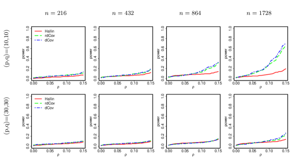
Figure C.9: Empirical powers of the three competing tests in Example C.1. The $y$-axis represents the power based on 1,000 replicates and the $x$-axis represents the level of a desired signal.

Table C.4: Empirical powers of the proposed test as well as two competing tests in Example C.2.

$(p,q)$	$n$	Hallin	rdCov	dCov
$(2,2)$	$54$	1.000	1.000	1.000
$(2,2)$	$108$	1.000	1.000	1.000
$(2,2)$	$216$	1.000	1.000	1.000
$(2,2)$	$432$	1.000	1.000	1.000
$(3,3)$	$54$	0.777	0.997	0.981
$(3,3)$	$108$	1.000	1.000	1.000
$(3,3)$	$216$	1.000	1.000	1.000
$(3,3)$	$432$	1.000	1.000	1.000
$(5,5)$	$54$	0.238	0.811	0.693
$(5,5)$	$108$	0.888	1.000	1.000
$(5,5)$	$216$	1.000	1.000	1.000
$(5,5)$	$432$	1.000	1.000	1.000
$(7,7)$	$54$	0.144	0.612	0.436
$(7,7)$	$108$	0.496	0.973	0.950
$(7,7)$	$216$	0.998	1.000	1.000
$(7,7)$	$432$	1.000	1.000	1.000

References

- Abe, (1969) Abe, O. (1969). A central limit theorem for the number of edges in the random intersection of two graphs. Ann. Math. Statist., 40(1):144–151.
- Agarwal and Sharathkumar, (2014) Agarwal, P. K. and Sharathkumar, R. (2014). Approximation algorithms for bipartite matching with metric and geometric costs. In STOC’14—Proceedings of the 2014 ACM Symposium on Theory of Computing, pages 555–564. ACM, New York, NY.
- Anselone, (1971) Anselone, P. M. (1971). Collectively compact operator approximation theory and applications to integral equations. Prentice-Hall, Inc., Englewood Cliffs, NJ.
- Atkinson, (1967) Atkinson, K. E. (1967). The numerical solutions of the eigenvalue problem for compact integral operators. Trans. Amer. Math. Soc., 129:458–465.
- Bakirov et al., (2006) Bakirov, N. K., Rizzo, M. L., and Székely, G. J. (2006). A multivariate nonparametric test of independence. J. Multivariate Anal., 97(8):1742–1756.
- Barbour and Chen, (2005) Barbour, A. D. and Chen, L. H. Y. (2005). The permutation distribution of matrix correlation statistics. In Stein’s Method and Applications, volume 5 of Lect. Notes Ser. Inst. Math. Sci. Natl. Univ. Singap., pages 223–245. Singapore Univ. Press, Singapore.
- Barbour and Eagleson, (1986) Barbour, A. D. and Eagleson, G. K. (1986). Random association of symmetric arrays. Stochastic Anal. Appl., 4(3):239–281.
- Basu, (1959) Basu, D. (1959). The family of ancillary statistics. Sankhyā, 21(3/4):247–256.
- Bergsma, (2006) Bergsma, W. (2006). A new correlation coefficient, its orthogonal decomposition and associated tests of independence. Available at arXiv:math/0604627v1.
- Bergsma and Dassios, (2014) Bergsma, W. and Dassios, A. (2014). A consistent test of independence based on a sign covariance related to Kendall’s tau. Bernoulli, 20(2):1006–1028.
- Berrett and Samworth, (2019) Berrett, T. B. and Samworth, R. J. (2019). Nonparametric independence testing via mutual information. Biometrika, 106(3):547–566.
- Beyer, (1987) Beyer, W. H., editor (1987). CRC handbook of mathematical sciences (6th ed.). CRC Press, Boca Raton, FL.
- Billingsley, (1995) Billingsley, P. (1995). Probability and measure (3rd ed.). Wiley Series in Probability and Mathematical Statistics. John Wiley & Sons, Inc., New York, NY.
- Billingsley, (1999) Billingsley, P. (1999). Convergence of probability measures (2nd ed.). Wiley Series in Probability and Statistics. John Wiley & Sons, Inc., New York, NY.
- Bloemena, (1964) Bloemena, A. R. (1964). Sampling from a graph. W. R. van Zwet (Ed.). Mathematical Centre Tracts, No. 2. Mathematisch Centrum, Amsterdam, Netherlands.
- Blum et al., (1961) Blum, J. R., Kiefer, J., and Rosenblatt, M. (1961). Distribution free tests of independence based on the sample distribution function. Ann. Math. Statist., 32:485–498.
- Blumenson, (1960) Blumenson, L. E. (1960). Classroom Notes: A Derivation of -Dimensional Spherical Coordinates. Amer. Math. Monthly, 67(1):63–66.
- Bolthausen, (1984) Bolthausen, E. (1984). An estimate of the remainder in a combinatorial central limit theorem. Z. Wahrsch. Verw. Gebiete, 66(3):379–386.
- Bolthausen and Götze, (1993) Bolthausen, E. and Götze, F. (1993). The rate of convergence for multivariate sampling statistics. Ann. Statist., 21(4):1692–1710.
- Chernozhukov et al., (2017) Chernozhukov, V., Galichon, A., Hallin, M., and Henry, M. (2017). Monge-Kantorovich depth, quantiles, ranks and signs. Ann. Statist., 45(1):223–256.
- Cliff and Ord, (1973) Cliff, A. D. and Ord, J. K. (1973). Spatial autocorrelation. Monographs in spatial and environmental systems analysis, 5. Pion, London, England.
- Cucker and Smale, (2002) Cucker, F. and Smale, S. (2002). On the mathematical foundations of learning. Bull. Amer. Math. Soc. (N.S.), 39(1):1–49.
- Daniels, (1944) Daniels, H. E. (1944). The relation between measures of correlation in the universe of sample permutations. Biometrika, 33(2):129–135.
- Deb and Sen, (2019) Deb, N. and Sen, B. (2019). Multivariate rank-based distribution-free nonparametric testing using measure transportation. Available at arXiv:1909.08733.
- DeGroot and Schervish, (2012) DeGroot, M. H. and Schervish, M. J. (2012). Probability and statistics (4th ed.). Addison-Wesley, Boston, MA.
- del Barrio et al., (2018) del Barrio, E., Cuesta-Albertos, J. A., Hallin, M., and Matrán, C. (2018). Smooth cyclically monotone interpolation and empirical center-outward distribution functions. Available at arXiv:1806.01238v1.
- Drton et al., (2020) Drton, M., Han, F., and Shi, H. (2020+). High dimensional consistent independence testing with maxima of rank correlations. Ann. Statist. (in press).
- Escanciano, (2006) Escanciano, J. C. (2006). A consistent diagnostic test for regression models using projections. Econometric Theory, 22(6):1030–1051.
- Fang et al., (1990) Fang, K. T., Kotz, S., and Ng, K. W. (1990). Symmetric multivariate and related distributions, volume 36 of Monographs on Statistics and Applied Probability. Chapman and Hall, Ltd., London, England.
- Farebrother, (1984) Farebrother, R. W. (1984). Algorithm AS 204: The distribution of a positive linear combination of random variables. J. Roy. Statist. Soc. Ser. C, 33(3):332–339.
- Feuerverger, (1993) Feuerverger, A. (1993). A consistent test for bivariate dependence. Int. Stat. Rev., 61(3):419–433.
- Figalli, (2018) Figalli, A. (2018). On the continuity of center-outward distribution and quantile functions. Nonlinear Anal., 177(part B):413–421.
- Gabow and Tarjan, (1989) Gabow, H. N. and Tarjan, R. E. (1989). Faster scaling algorithms for network problems. SIAM J. Comput., 18(5):1013–1036.
- Gebelein, (1941) Gebelein, H. (1941). Das statistische Problem der Korrelation als Variations- und Eigenwertproblem und sein Zusammenhang mit der Ausgleichsrechnung. Z. Angew. Math. Mech., 21:364–379.
- Ghosal and Sen, (2019) Ghosal, P. and Sen, B. (2019). Multivariate ranks and quantiles using optimal transportation and applications to goodness-of-fit testing. Available at arXiv:1905.05340.
- (36) Gretton, A., Bousquet, O., Smola, A., and Schölkopf, B. (2005a). Measuring statistical dependence with Hilbert-Schmidt norms. In Algorithmic learning theory, volume 3734 of Lecture Notes in Comput. Sci., pages 63–77. Springer-Verlag Berlin Heidelberg, Berlin, Germany.
- Gretton et al., (2008) Gretton, A., Fukumizu, K., Teo, C. H., Song, L., Schölkopf, B., and Smola, A. J. (2008). A kernel statistical test of independence. In Platt, J. C., Koller, D., Singer, Y., and Roweis, S. T., editors, Advances in Neural Information Processing Systems 20, pages 984–991. Curran Associates, Inc., Red Hook, NY.
- (38) Gretton, A., Herbrich, R., Smola, A., Bousquet, O., and Schölkopf, B. (2005b). Kernel methods for measuring independence. J. Mach. Learn. Res., 6(Dec):2075–2129.
- (39) Gretton, A., Smola, A., Bousquet, O., Herbrich, R., Belitski, A., Augath, M., Murayama, Y., Pauls, J., Schölkopf, B., and Logothetis, N. (2005c). Kernel constrained covariance for dependence measurement. In Cowell, R. G. and Ghahramani, Z., editors, AISTATS05, pages 112–119. Society for Artificial Intelligence and Statistics.
- Hájek, (1961) Hájek, J. (1961). Some extensions of the Wald–Wolfowitz–Noether theorem. Ann. Math. Statist., 32(2):506–523.
- Hallin, (2017) Hallin, M. (2017). On distribution and quantile functions, ranks and signs in : a measure transportation approach. Available at https://ideas.repec.org/p/eca/wpaper/2013-258262.html.
- Hallin et al., (2020) Hallin, M., del Barrio, E., Cuesta-Albertos, J. A., and Matrán, C. (2020). Distribution and quantile functions, ranks, and signs in dimension : a measure transportation approach. Available at arXiv:1806.01238v3.
- (43) Hallin, M. and Paindaveine, D. (2002a). Multivariate signed ranks: Randles’ interdirections or Tyler’s angles? In Statistical Data Analysis Based on the -Norm and Related Methods (Neuchâtel, 2002), Stat. Ind. Technol., pages 271–282. Birkhäuser, Basel.
- (44) Hallin, M. and Paindaveine, D. (2002b). Optimal tests for multivariate location based on interdirections and pseudo-Mahalanobis ranks. Ann. Statist., 30(4):1103–1133.
- Heller et al., (2012) Heller, R., Gorfine, M., and Heller, Y. (2012). A class of multivariate distribution-free tests of independence based on graphs. J. Statist. Plann. Inference, 142(12):3097–3106.
- Heller and Heller, (2016) Heller, R. and Heller, Y. (2016). Multivariate tests of association based on univariate tests. In Lee, D. D., Sugiyama, M., Luxburg, U. V., Guyon, I., and Garnett, R., editors, Advances in Neural Information Processing Systems 29, pages 208–216. Curran Associates, Inc.
- Heller et al., (2013) Heller, R., Heller, Y., and Gorfine, M. (2013). A consistent multivariate test of association based on ranks of distances. Biometrika, 100(2):503–510.
- Heller et al., (2016) Heller, R., Heller, Y., Kaufman, S., Brill, B., and Gorfine, M. (2016). Consistent distribution-free -sample and independence tests for univariate random variables. J. Mach. Learn. Res., 17(29):1–54.
- Hirschfeld, (1935) Hirschfeld, H. O. (1935). A connection between correlation and contingency. Mathematical Proceedings of the Cambridge Philosophical Society, 31(4):520–524.
- Hoeffding, (1940) Hoeffding, W. (1940). Maszstabinvariante Korrelationstheorie. Schr. Math. Inst. u. Inst. Angew. Math. Univ. Berlin, 5:181–233.
- Hoeffding, (1948) Hoeffding, W. (1948). A non-parametric test of independence. Ann. Math. Statist., 19(4):546–557.
- Hoeffding, (1951) Hoeffding, W. (1951). A combinatorial central limit theorem. Ann. Math. Statist., 22(4):558–566.
- Hopcroft and Karp, (1973) Hopcroft, J. E. and Karp, R. M. (1973). An algorithm for maximum matchings in bipartite graphs. SIAM J. Comput., 2(4):225–231.
- Huo and Székely, (2016) Huo, X. and Székely, G. J. (2016). Fast computing for distance covariance. Technometrics, 58(4):435–447.
- Imhof, (1961) Imhof, J. P. (1961). Computing the distribution of quadratic forms in normal variables. Biometrika, 48(3/4):419–426.
- Jakobsen, (2017) Jakobsen, M. E. (2017). Distance covariance in metric spaces: Non-parametric independence testing in metric spaces. Master’s thesis, University of Copenhagen. Available at arXiv:1706.03490.
- Jogdeo, (1968) Jogdeo, K. (1968). Asymptotic normality in nonparametric methods. Ann. Math. Statist., 39(3):905–922.
- Kim et al., (2018) Kim, I., Balakrishnan, S., and Wasserman, L. (2018). Robust multivariate nonparametric tests via projection-pursuit. Available at arXiv:1803.00715.
- Kinney and Atwal, (2014) Kinney, J. B. and Atwal, G. S. (2014). Equitability, mutual information, and the maximal information coefficient. Proc. Natl. Acad. Sci. USA, 111(9):3354–3359.
- König, (1986) König, H. (1986). Eigenvalue distribution of compact operators, volume 16 of Operator Theory: Advances and Applications. Birkhäuser Verlag, Basel, Switzerland.
- Koroljuk and Borovskich, (1994) Koroljuk, V. S. and Borovskich, Y. V. (1994). Theory of -statistics (P. V. Malyshev and D. V. Malyshev, Trans.), volume 273 of Mathematics and its Applications. Kluwer Academic Publishers Group, Dordrecht, Netherlands.
- Kraskov et al., (2004) Kraskov, A., Stögbauer, H., and Grassberger, P. (2004). Estimating mutual information. Phys. Rev. E, 69(6):066138, 1–16.
- Kuhn, (1955) Kuhn, H. W. (1955). The Hungarian method for the assignment problem. Naval Res. Logist. Quart., 2(1–2):83–97.
- Kuhn, (1956) Kuhn, H. W. (1956). Variants of the Hungarian method for assignment problems. Naval Res. Logist. Quart., 3(4):253–258.
- Lin, (2017) Lin, J. (2017). Copula versions of RKHS-based and distance-based criteria. PhD thesis, Pennsylvania State University. Available at https://etda.libraries.psu.edu/catalog/14485jul268.
- Lyons, (2013) Lyons, R. (2013). Distance covariance in metric spaces. Ann. Probab., 41(5):3284–3305.
- Lyons, (2018) Lyons, R. (2018). Errata to “Distance covariance in metric spaces”. Ann. Probab., 46(4):2400–2405.
- Ma and Mao, (2019) Ma, L. and Mao, J. (2019). Fisher exact scanning for dependency. J. Amer. Statist. Assoc., 114(525):245–258.
- McCann, (1995) McCann, R. J. (1995). Existence and uniqueness of monotone measure-preserving maps. Duke Math. J., 80(2):309–323.
- Motoo, (1957) Motoo, M. (1957). On the Hoeffding’s combinatorial central limit theorem. Ann. Inst. Statist. Math. Tokyo, 8(3):145–154.
- Munkres, (1957) Munkres, J. (1957). Algorithms for the assignment and transportation problems. J. Soc. Indust. Appl. Math., 5(1):32–38.
- Nandy et al., (2016) Nandy, P., Weihs, L., and Drton, M. (2016). Large-sample theory for the Bergsma–Dassios sign covariance. Electron. J. Stat., 10(2):2287–2311.
- Noether, (1949) Noether, G. E. (1949). On a theorem of Wald and Wolfowitz. Ann. Math. Statist., 20(3):455–458.
- Pan et al., (2020) Pan, W., Wang, X., Zhang, H., Zhu, H., and Zhu, J. (2020). Ball Covariance: A Generic Measure of Dependence in Banach Space. J. Amer. Statist. Assoc., 115(529):307–317.
- Pham et al., (1989) Pham, D. T., Möcks, J., and Sroka, L. (1989). Asymptotic normality of double-indexed linear permutation statistics. Ann. Inst. Statist. Math., 41(3):415–427.
- Raic̆, (2015) Raic̆, M. (2015). Multivariate normal approximation: permutation statistics, local dependence and beyond. Available at http://www2.ims.nus.edu.sg/Programs/015wstein/files/martin.pdf.
- Reinert and Röllin, (2009) Reinert, G. and Röllin, A. (2009). Multivariate normal approximation with Stein’s method of exchangeable pairs under a general linearity condition. Ann. Probab., 37(6):2150–2173.
- Rémillard, (2009) Rémillard, B. (2009). Discussion of: Brownian distance covariance. Ann. Appl. Stat., 3(4):1295–1298.
- (79) Rényi, A. (1959a). New version of the probabilistic generalization of the large sieve. Acta Math. Acad. Sci. Hungar., 10(1–2):217–226.
- (80) Rényi, A. (1959b). On measures of dependence. Acta Math. Acad. Sci. Hungar., 10(3–4):441–451.
- Reshef et al., (2011) Reshef, D. N., Reshef, Y. A., Finucane, H. K., Grossman, S. R., McVean, G., Turnbaugh, P. J., Lander, E. S., Mitzenmacher, M., and Sabeti, P. C. (2011). Detecting novel associations in large data sets. Science, 334(6062):1518–1524.
- Reshef et al., (2018) Reshef, D. N., Reshef, Y. A., Sabeti, P. C., and Mitzenmacher, M. (2018). An empirical study of the maximal and total information coefficients and leading measures of dependence. Ann. Appl. Stat., 12(1):123–155.
- Reshef et al., (2016) Reshef, Y. A., Reshef, D. N., Finucane, H. K., Sabeti, P. C., and Mitzenmacher, M. (2016). Measuring dependence powerfully and equitably. J. Mach. Learn. Res., 17(211):1–63.
- Rudin, (1976) Rudin, W. (1976). Principles of mathematical analysis (3rd ed.). International Series in Pure and Applied Mathematics. McGraw-Hill Book Co., New York, NY.
- Rudin, (1987) Rudin, W. (1987). Real and complex analysis (3rd ed.). McGraw-Hill Book Co., New York, NY.
- Sejdinovic et al., (2013) Sejdinovic, D., Sriperumbudur, B., Gretton, A., and Fukumizu, K. (2013). Equivalence of distance-based and RKHS-based statistics in hypothesis testing. Ann. Statist., 41(5):2263–2291.
- Serfling, (1980) Serfling, R. J. (1980). Approximation theorems of mathematical statistics. Wiley Series in Probability and Mathematical Statistics. John Wiley & Sons, Inc., New York, NY.
- Shapiro and Hubert, (1979) Shapiro, C. P. and Hubert, L. (1979). Asymptotic normality of permutation statistics derived from weighted sums of bivariate functions. Ann. Statist., 7(4):788–794.
- Sharathkumar and Agarwal, (2012) Sharathkumar, R. and Agarwal, P. K. (2012). Algorithms for the transportation problem in geometric settings. In Proceedings of the Twenty-Third Annual ACM-SIAM Symposium on Discrete Algorithms, pages 306–317, New York, NY. ACM.
- (90) Simon, B. (2015a). Operator theory. A Comprehensive Course in Analysis, Part 4. American Mathematical Society, Providence, RI.
- (91) Simon, B. (2015b). Real analysis. A Comprehensive Course in Analysis, Part 1. American Mathematical Society, Providence, RI.
- Székely and Bakirov, (2003) Székely, G. J. and Bakirov, N. K. (2003). Extremal probabilities for Gaussian quadratic forms. Probab. Theory Related Fields, 126(2):184–202.
- Székely and Rizzo, (2009) Székely, G. J. and Rizzo, M. L. (2009). Brownian distance covariance. Ann. Appl. Stat., 3(4):1236–1265.
- Székely and Rizzo, (2013) Székely, G. J. and Rizzo, M. L. (2013). The distance correlation -test of independence in high dimension. J. Multivariate Anal., 117:193–213.
- Székely and Rizzo, (2014) Székely, G. J. and Rizzo, M. L. (2014). Partial distance correlation with methods for dissimilarities. Ann. Statist., 42(6):2382–2412.
- Székely et al., (2007) Székely, G. J., Rizzo, M. L., and Bakirov, N. K. (2007). Measuring and testing dependence by correlation of distances. Ann. Statist., 35(6):2769–2794.
- van der Vaart, (1998) van der Vaart, A. W. (1998). Asymptotic statistics, volume 3 of Cambridge Series in Statistical and Probabilistic Mathematics. Cambridge University Press, Cambridge, United Kingdom.
- Villani, (2009) Villani, C. (2009). Optimal transport: Old and new, volume 338 of Grundlehren der Mathematischen Wissenschaften [Fundamental Principles of Mathematical Sciences]. Springer-Verlag Berlin Heidelberg, Berlin, Germany.
- Wald and Wolfowitz, (1944) Wald, A. and Wolfowitz, J. (1944). Statistical tests based on permutations of the observations. Ann. Math. Statist., 15(4):358–372.
- Weihs et al., (2018) Weihs, L., Drton, M., and Meinshausen, N. (2018). Symmetric rank covariances: a generalized framework for nonparametric measures of dependence. Biometrika, 105(3):547–562.
- Yanagimoto, (1970) Yanagimoto, T. (1970). On measures of association and a related problem. Ann. Inst. Statist. Math., 22(1):57–63.
- (102) Yao, S., Zhang, X., and Shao, X. (2018a). Supplementary material for “Testing mutual independence in high dimension via distance covariance”. J. R. Stat. Soc. Ser. B. Stat. Methodol., 80(3).
- (103) Yao, S., Zhang, X., and Shao, X. (2018b). Testing mutual independence in high dimension via distance covariance. J. R. Stat. Soc. Ser. B. Stat. Methodol., 80(3):455–480.
- Zhang, (2019) Zhang, K. (2019+). BET on independence. J. Amer. Statist. Assoc., (in press):1–18.
- Zhao et al., (1997) Zhao, L., Bai, Z., Chao, C.-C., and Liang, W.-Q. (1997). Error bound in a central limit theorem of double-indexed permutation statistics. Ann. Statist., 25(5):2210–2227.
- Zhu et al., (2017) Zhu, L., Xu, K., Li, R., and Zhong, W. (2017). Projection correlation between two random vectors. Biometrika, 104(4):829–843.