Robust Field-Only Surface Integral Equations: Scattering from a Dielectric Body

A robust and efficient field-only nonsingular surface integral method to solve Maxwell’s equations for the components of the electric field on the surface of a dielectric scatterer is introduced. In this method, both the vector Helmholtz equation and the divergence-free constraint are satisfied inside and outside the scatterer. The divergence-free condition is replaced by an equivalent boundary condition that relates the normal derivatives of the electric field across the surface of the scatterer. Also, the continuity and jump conditions on the electric and magnetic fields are expressed in terms of the electric field across the surface of the scatterer. Together with these boundary conditions, the scalar Helmholtz equation for the components of the electric field inside and outside the scatterer is solved by a fully desingularized surface integral method. Comparing with the most popular surface integral methods based on the Stratton–Chu formulation or the PMCHWT formulation, our method is conceptually simpler and numerically straightforward because there is no need to introduce intermediate quantities such as surface currents and the use of complicated vector basis functions can be avoided altogether. Also, our method is not affected by numerical issues such as the zero frequency catastrophe and does not contain integrals with (strong) singularities. To illustrate the robustness and versatility of our method, we show examples in the Rayleigh, Mie, and geometrical optics scattering regimes. Given the symmetry between the electric field and the magnetic field, our theoretical framework can also be used to solve for the magnetic field.

1 Introduction

There have been two recent independent developments in formulating computational electromagnetics (CEM) scattering [1] in terms of surface integral equations [2, 3] that are conceptually very different from the venerable theoretical framework of Stratton–Chu which was established almost 80 years ago [4, 5] or the PMCHWT formulation [6, 7, 8] or the potential based CEM methods [9, 10]. These earlier methods either entail solving for surface currents or charges at boundaries or for the scalar and vector potentials, whereas the recent works are based on solving directly for components of the electric field. One of the field-only formulations had its genesis in the study of scattering from (i) infinite rough surfaces [11] some 25 years ago, (ii) finite dielectric bodies [12] more than a decade ago, and has been recently generalized with an extensive use of differential geometry [2]. The other field-only formulation [3, 13] focused on the use of nonsingular surface integral equations for the field components. This method stems from an observation that the physical phenomena is finite and well-behaved on boundaries, and thus should not contain mathematically singular kernels. In this method, the divergence-free condition was satisfied via the identity

$$\nabla^{2}(\boldsymbol{r}\cdot\boldsymbol{E})+k^{2}(\boldsymbol{r}\cdot\boldsymbol{E})=2\boldsymbol{\nabla}\cdot\boldsymbol{E}=0,$$

where $\boldsymbol{r}$ the position vector, and resulted in an additional Helmholtz equation for $\boldsymbol{r}\cdot\boldsymbol{E}$ that led to a $9N\times 9N$ system of linear equations [13].

In this paper, we combine the above two field-only integral methods to obtain a nonsingular integral formulation, which when discretized yields a $6N\times 6N$ system of linear equations. Therefore, the framework developed in this paper gives a $56\%$ reduction in memory requirements and subsequently leads to faster solution times. Furthermore, this approach turns out to be conceptually simple and can provide direct access to values of the field and its normal derivatives on the boundary of the scatterer. The implementation is free of mathematical singularities and facilitates the use of simple, efficient and accurate surface integration algorithms. It also should be noted that this paper is a natural generalization of our previous publication [14]. In [14], we considered the much simpler case of scattering by a perfect electric conductor (PEC) in order not to obscure the conceptual simplicity and elegance of the method by the non-zero internal fields.

The paper is organized as follows. The theoretical framework of our formulation is explained in Section 2. In Section 3, we consider numerical examples of interest to the optics community in the Rayleigh, Mie, and geometric optics scattering regimes. Finally, some concluding remarks are presented in Section 4 as well as a prescription how to modify our formulation if the magnetic fields are of primary interest.

2 Field-Only Formulation

In a source-free, linear, homogeneous medium the propagation of a time-harmonic electric field $\boldsymbol{E}(\boldsymbol{r})\exp(-\mathrm{i}\omega t)$, with $t$ denoting time and $\omega$ denoting the angular frequency, is governed by the vector Helmholtz equation

$$\nabla^{2}\boldsymbol{E}(\boldsymbol{r})+k^{2}\boldsymbol{E}(\boldsymbol{r})=\boldsymbol{0},$$ (1)

where $k=\sqrt{\epsilon\mu}\omega$ is the wavenumber with $\epsilon$ and $\mu$ being the permittivity and permeability of the medium, respectively. Thus, each Cartesian component of $\boldsymbol{E}$ satisfies the scalar Helmholtz wave equation

$$\nabla^{2}E_{\alpha}+k^{2}E_{\alpha}=0,\qquad\alpha=x,y,z.$$ (2)

The electric field is also divergence-free, i.e.,

$$\boldsymbol{\nabla}\cdot\boldsymbol{E}=0,$$ (3)

thus, in principle there are only two independent components of $\boldsymbol{E}$ that have to be determined.

In a typical scattering problem, an incident wave, $\boldsymbol{E}^{\mathrm{inc}}$, is scattered by a dielectric body, and the resulting scattered field outside the scatterer as well as the transmitted field inside the scatterer are to be determined. After accounting for the fact that the scattered field, $\boldsymbol{E}^{\mathrm{sc}}$, obeys the Silver–Müller radiation condition [15], the transmitted field, $\boldsymbol{E}^{\mathrm{tr}}$, is finite inside the scatterer, and both $\boldsymbol{E}^{\mathrm{sc}}$ and $\boldsymbol{E}^{\mathrm{tr}}$ satisfy (3), we see that there are only four unknown scalar functions (two for each domain). These functions are usually found by solving (2) and applying the continuity conditions for the tangential components of the electric and magnetic fields. In our formulation, the key point of departure from the formulation outlined above is to cast the divergence-free condition in the 3D domain as a boundary condition. Since the problem is elliptic in nature, this should always be possible. Casting the divergence-free condition as a boundary condition enables us to directly solve for the components of $\boldsymbol{E}$. Furthermore, it guarantees that $\boldsymbol{E}^{\mathrm{sc}}$ ($\boldsymbol{E}^{\mathrm{tr}}$) satisfies the divergence-free condition in the 3D domain outside (inside) the scatterer [2, 14].

The value of $\boldsymbol{\nabla}\cdot\boldsymbol{E}$ on the scatterer’s surface $S$ can be expressed using differential geometry as a combination of the normal component of $\boldsymbol{E}$ on $S$ and the normal as well as the tangential derivatives of $\boldsymbol{E}$ on $S$ (see [14, equation (A12)] or [2, equation (23)]). That is, at any point on the surface $S$, we have

$$\boldsymbol{\nabla}\cdot\boldsymbol{E}=\boldsymbol{n}\cdot\frac{\partial\boldsymbol{E}}{\partial{n}}-\kappa E_{n}+\frac{\partial{E_{t_{1}}}}{\partial{t_{1}}}+\frac{\partial{E_{t_{2}}}}{\partial{t_{2}}}=0,$$ (4)

where $\kappa$ is the mean curvature. In (4), $\boldsymbol{n}$ is the unit normal pointing into the scatterer, $E_{n}=\boldsymbol{n}\cdot\boldsymbol{E}$ is the normal component of $\boldsymbol{E}$, and $E_{t_{1}}=\boldsymbol{t}_{1}\cdot\boldsymbol{E}$ and $E_{t_{2}}=\boldsymbol{t}_{2}\cdot\boldsymbol{E}$ are the tangential components of $\boldsymbol{E}$ along the two mutually perpendicular tangential unit vectors $\boldsymbol{t}_{1}$ and $\boldsymbol{t}_{2}$. The normal and tangential derivatives are defined by $\partial(\cdot)/\partial n=\boldsymbol{n}\cdot\boldsymbol{\nabla}(\cdot)$ and $\partial(\cdot)/\partial t_{j}=\boldsymbol{t}_{j}\cdot\boldsymbol{\nabla}(\cdot)$ for $j=1,2$, respectively.

We will use (4) to decompose the standard surface integral representation written for the three Cartesian components of the electric field into its normal and tangential components. Outside the scatterer we use Green’s second identity to express the solution of (2) for the scattered field, $\boldsymbol{E}^{\mathrm{sc}}(\boldsymbol{r}_{0})$, in terms of integrals over the surface values

$$c_{0}(\boldsymbol{r}_{0})E^{\mathrm{sc}}_{\alpha}(\boldsymbol{r}_{0})+\int_{S}E^{\mathrm{sc}}_{\alpha}(\boldsymbol{r})\frac{\partial G(\boldsymbol{r},\boldsymbol{r}_{0})}{\partial n}\,\mathrm{d}S(\boldsymbol{r})=\int_{S}\frac{\partial E^{\mathrm{sc}}_{\alpha}(\boldsymbol{r})}{\partial n}G(\boldsymbol{r},\boldsymbol{r}_{0})\,\mathrm{d}S(\boldsymbol{r}),\quad\alpha=x,y,z,$$ (5a)

where $$c_{0}=4\pi \boldsymbol{r}_{0}\notin S \boldsymbol{r}_{0} \boldsymbol{r}_{0}\in S c_{0} \boldsymbol{r}_{0} \boldsymbol{E}^{\mathrm{tr}}$$ if (i.e., when is in the 3D domain outside the scatterer). If (approached from the exterior 3D domain), then is the solid angle subtended at . The integral representation of the transmitted field, , inside the scatterer is given by

$$c_{0}^{\mathrm{in}}(\boldsymbol{r}_{0})E^{\mathrm{tr}}_{\alpha}(\boldsymbol{r}_{0})-\int_{S}E^{\mathrm{tr}}_{\alpha}(\boldsymbol{r})\frac{\partial G_{\mathrm{in}}(\boldsymbol{r},\boldsymbol{r}_{0})}{\partial n}\,\mathrm{d}S(\boldsymbol{r})=-\int_{S}\frac{\partial E^{\mathrm{tr}}_{\alpha}(\boldsymbol{r})}{\partial n}G_{\mathrm{in}}(\boldsymbol{r},\boldsymbol{r}_{0})\,\mathrm{d}S(\boldsymbol{r}),\quad\alpha=x,y,z,$$ (5b)

where $\boldsymbol{r}_{0}$ is inside the scatterer. Equation (5b) follows directly from the application of Green’s second identity to (2) with $E_{\alpha}=E_{\alpha}^{\mathrm{tr}}$ and the two minus signs appear because the normal vector points into the scatterer. In (5b), $c_{0}^{\mathrm{in}}=4\pi$ if $\boldsymbol{r}_{0}\notin S$ (i.e., $\boldsymbol{r}_{0}$ is inside the scatterer) and $c_{0}^{\mathrm{in}}$ is the solid angle if $\boldsymbol{r}_{0}\in S$ when $\boldsymbol{r}_{0}$ approaches to $S$ from inside the scatterer. It is worth mentioning that $c_{0}+c_{0}^{\mathrm{in}}=4\pi$ if $\boldsymbol{r}_{0}\in S$. In (5), Green’s function is $G(\boldsymbol{r},\boldsymbol{r}_{0})=\exp(\mathrm{i}k|\boldsymbol{r}-\boldsymbol{r}_{0}|/|\boldsymbol{r}-\boldsymbol{r}_{0}|,$ where $k$ denotes the appropriate wavenumber for the region, i.e., $k=k_{\mathrm{in}}=\sqrt{\epsilon_{\mathrm{in}}\mu_{\mathrm{in}}}\omega$ for $G_{\mathrm{in}}(\boldsymbol{r},\boldsymbol{r}_{0})$ (inside the scatterer) or $k=k_{\mathrm{out}}=\sqrt{\epsilon_{\mathrm{out}}\mu_{\mathrm{out}}}\omega$ for $G(\boldsymbol{r},\boldsymbol{r}_{0})$ (outside the scatterer) .

At this point in the formulation, we see that (5) contains $12$ unknown functions on $S$; namely, $\{E_{\alpha}^{\mathrm{sc}},\partial E_{\alpha}^{\mathrm{sc}}/\partial n\}$ and $\{E_{\alpha}^{\mathrm{sc}}$, $\partial E_{\alpha}^{\mathrm{sc}}/\partial n\}$, $\alpha=x,y,z$. In order to determine the $12$ unknown functions we need 12 equations. Six of these equations come from (5). Three more equations come from the continuity conditions satisfied by the electric field on $S$, namely,

$$E_{n}^{\mathrm{tr}}=\epsilon_{\mathrm{oi}}(E_{n}^{\mathrm{inc}}+E_{n}^{\mathrm{sc}}),\quad\epsilon_{\mathrm{oi}}\equiv\epsilon_{\mathrm{out}}/\epsilon_{\mathrm{in}}$$ (6a)

and

$$E_{t_{j}}^{\mathrm{inc}}+E_{t_{j}}^{\mathrm{sc}}=E_{t_{j}}^{\mathrm{tr}},\quad j=1,2.$$ (6b)

The last three equations come from the continuity condition satisfied by the normal derivative of the electric field, $\partial\boldsymbol{E}/\partial n$, on $S$.

To derive these last three equations, we write (4) for the total exterior field, $\boldsymbol{E}^{\mathrm{sc}}+\boldsymbol{E}^{\mathrm{inc}}$, and subtract the corresponding equation for the transmitted field, $\boldsymbol{E}^{\mathrm{tr}}$. Then, after using (6), we obtain

$$\boldsymbol{n}\cdot\frac{\partial{\boldsymbol{E}^{\mathrm{tr}}}}{\partial{n}}=\kappa(\epsilon_{\mathrm{oi}}-1)\left(E^{\mathrm{sc}}_{n}+E^{\mathrm{inc}}_{n}\right)+\boldsymbol{n}\cdot\frac{\partial{\boldsymbol{E}^{\mathrm{sc}}}}{\partial{n}}+\boldsymbol{n}\cdot\frac{\partial{\boldsymbol{E}^{\mathrm{inc}}}}{\partial{n}}.$$ (7a)

Equation (7a) only provides a continuity condition for the normal component of $$\partial\boldsymbol{E}/\partial n \partial\boldsymbol{E}/\partial n \boldsymbol{H} S$$. To obtain a continuity condition for the tangential components of , we express the continuity condition for the tangential components of on , i.e.,

$$H_{t_{j}}^{\mathrm{inc}}+H_{t_{j}}^{\mathrm{sc}}=H_{t_{j}}^{\mathrm{tr}}\quad\text{for}\quad j=1,2,$$ (7b)

in terms of the electric field to obtain (see Appendix A for details)

$$\left(\epsilon_{\mathrm{oi}}-\mu_{\mathrm{io}}\right)\frac{\partial}{\partial t_{j}}\left[E_{n}^{\mathrm{inc}}+E_{n}^{\mathrm{sc}}\right]+\kappa_{j}\left(1-\mu_{\mathrm{io}}\right)\left[E_{t_{j}}^{\mathrm{inc}}+E_{t_{j}}^{\mathrm{sc}}\right]\\ +\mu_{\mathrm{io}}\left(\boldsymbol{t}_{j}\cdot\frac{\partial\boldsymbol{E}^{\mathrm{inc}}}{\partial n}+\boldsymbol{t}_{j}\cdot\frac{\partial\boldsymbol{E}^{\mathrm{sc}}}{\partial n}\right)=\boldsymbol{t}_{j}\cdot\frac{\partial\boldsymbol{E}^{\mathrm{tr}}}{\partial n},$$ (7c)

where $\mu_{\mathrm{io}}\equiv\mu_{\mathrm{in}}/\mu_{\mathrm{out}}$, $\kappa_{j}$ is the local curvature along the $\boldsymbol{t}_{j}$ direction and $j=1,2$. In the limit $\mu_{\mathrm{io}}=1$, (7c) reduces to

$$\left(1-\epsilon_{\mathrm{oi}}^{-1}\right)\frac{\partial E_{n}^{\mathrm{tr}}}{\partial t_{j}}=\boldsymbol{t}_{j}\cdot\frac{\partial}{\partial n}\left[\boldsymbol{E}^{\mathrm{tr}}-\left(\boldsymbol{E}^{\mathrm{inc}}+\boldsymbol{E}^{\mathrm{sc}}\right)\right]$$ (8)

for $j=1,2$. Equation (8) states that in a nonmagnetic medium the tangential components of the normal derivative of the electric field are discontinuous across an interface by an amount proportional to the tangential derivative of the normal component of the electric field inside the scatterer. Furthermore, if there is no scatterer, i.e., $\epsilon_{\mathrm{oi}}=1$, then (8) reduces to the expected form; namely, $\boldsymbol{t}_{j}\cdot\frac{\partial}{\partial n}\left(\boldsymbol{E}^{\mathrm{inc}}+\boldsymbol{E}^{\mathrm{sc}}\right)=\boldsymbol{t}_{j}\cdot\frac{\partial}{\partial n}\boldsymbol{E}^{\mathrm{tr}}$ for $j=1,2$.

Lastly, we note that (6) and (7) are simply equations (9) and (19) in [2], respectively, written in a different notation. Furthermore, (7) (or equivalently equation (19) in [2]) is not widely known to the scientific community but is an essential equation for our surface integral method.

2.1 Numerical Solution

One approach to obtain a numerical solution is to directly discretize the surface integral equations given by (5) [16]. This approach will yield a system of linear equations that can be solved for the chosen unknowns: $\{E_{n}^{\mathrm{sc}},E_{t_{1}}^{\mathrm{sc}},E_{t_{2}}^{\mathrm{sc}}\}$ and $\{\boldsymbol{n}\cdot\partial{\boldsymbol{E}^{\mathrm{sc}}}/{\partial{n}},\boldsymbol{t}_{1}\cdot\partial{\boldsymbol{E}^{\mathrm{sc}}}/{\partial{n}},\boldsymbol{t}_{2}\cdot\partial{\boldsymbol{E}^{\mathrm{sc}}}/{\partial{n}}\}$. Unfortunately, this approach requires the discretization of singular kernels (Green’s function and its normal derivative) and, therefore, much care must be taken to avoid numerical difficulties [16]. Another approach would be to use our recently developed robust and accurate desingularized method [3, 13], where the singular behavior of Green’s function and its normal derivative is “subtracted out” before the discretization. This is the method we have chosen to use here and it is explained in more detail in Appendix B (also see [14]).

From Appendix B, we see that the nonsingular version of (5) is given by

$$\int_{\Sigma}{\left[\frac{\partial{p(\boldsymbol{r})}}{{\partial{n}}}-p(\boldsymbol{r}_{0})\frac{\partial{g(\boldsymbol{r})}}{{\partial{n}}}-\frac{\partial{p(\boldsymbol{r}_{0})}}{{\partial{n}}}\frac{\partial{f(\boldsymbol{r})}}{{\partial{n}}}\right]G\,\mathrm{d}S(\boldsymbol{r}})\\ =\int_{\Sigma}{\left[p(\boldsymbol{r})-p(\boldsymbol{r}_{0})g(\boldsymbol{r})-\frac{\partial{p(\boldsymbol{r}_{0})}}{{\partial{n}}}f(\boldsymbol{r})\right]\frac{\partial{G}}{{\partial{n}}}\,\mathrm{d}S(\boldsymbol{r}}),$$ (9)

where $f$ and $g$ are auxiliary functions that “subtract out” the singular behavior of the kernels. For the interior problem, $p$ is one of the Cartesian components of the transmitted field, i.e., $p=E_{\alpha}^{\mathrm{tr}},\alpha=x,y,z$, and $\Sigma=S$. Similarly, for the exterior problem, $p$ is one of the Cartesian components of the scattered field but $\Sigma=S+S_{\infty}$, where $S_{\infty}$ is an artificial sphere of infinite radius. Note that the contribution from $S_{\infty}$ is generally non-zero because $f$ and $g$ may not decay as fast as the scattered field at infinity. However, with our choice of $f$ and $g$ the integrals over $S_{\infty}$ may be performed analytically, and thus are not of much concern, see Appendix B.

For the exterior problem, after discretizing the surface $S$ into six-noded quadratic triangular elements [3, 13], the surface integral equation (9) is converted into a surface element matrix system connecting all $N$ nodes to their normal derivatives via

$${\cal{H}}\cdot\underline{p^{\mathrm{sc}}}={\cal{G}}\cdot\underline{\frac{\partial p^{\mathrm{sc}}}{\partial n}}$$ (10a)

In (10a), $$\underline{p^{\mathrm{sc}}}=\underline{E^{\mathrm{sc}}_{\alpha}} \alpha=x,y\text{ or }z N p^{\mathrm{sc}} \underline{\frac{\partial p^{\mathrm{sc}}}{\partial n}} p^{\mathrm{sc}} \cal{G} \cal{H} {\cal{H}}_{\mathrm{in}} {\cal{G}}_{\mathrm{in}} {\cal{H}} {\cal{G}} {\cal{H}}_{\mathrm{in}} {\cal{G}}_{\mathrm{in}} S_{\infty} k$$ (with ) represents a column vector with all of the node values of , is a similar column vector for the normal derivatives of . For explicit examples of and see Appendix B in [14]. Another matrix system can be constructed for the transmitted field (interior problem) but with and matrices which can also be obtained following the same procedure demonstrated in Appendix B in [14]. These matrices differ from and because and do not contain contributions from integrals over and the Green’s function inside the scatterer has a different wavenumber . For completeness and to facilitate the development that follows, we explicitly write this relationship as

$${\cal{H}}_{\mathrm{in}}\cdot\underline{p^{\mathrm{tr}}}={\cal{G}}_{\mathrm{in}}\cdot\underline{\frac{\partial p^{\mathrm{tr}}}{\partial n}},$$ (10b)

where $\underline{p^{\mathrm{tr}}}=\underline{E^{\mathrm{tr}}_{\alpha}}$ and $\alpha=x,y\text{ or }z$.

We need to use the boundary conditions given by (6) and (7) to eliminate $\underline{p^{\mathrm{tr}}}$ and $\underline{\frac{\partial p^{\mathrm{tr}}}{\partial n}}$ from (9). However, the boundary conditions are written in terms of the normal and tangential components and (9) requires the Cartesian components. To reconcile this mismatch, we project the normal and tangential basis onto the Cartesian basis $\{\boldsymbol{e}_{x},\boldsymbol{e}_{y},\boldsymbol{e}_{z}\}$, i.e.,

$$E_{\alpha}\boldsymbol{e}_{\alpha}=\left[n_{\alpha}E_{n}\right]\boldsymbol{e}_{\alpha}+\left[t_{1\alpha}E_{t_{1}}\right]\boldsymbol{e}_{\alpha}+\left[t_{2\alpha}E_{t_{2}}\right]\boldsymbol{e}_{\alpha},$$ (11a)

$$\frac{\partial E_{\alpha}}{\partial n}\boldsymbol{e}_{\alpha}=\left[n_{\alpha}\left(\boldsymbol{n}\cdot\frac{\partial\boldsymbol{E}}{\partial n}\right)\right]\boldsymbol{e}_{\alpha}+\left[t_{1\alpha}\left(\boldsymbol{t}_{1}\cdot\frac{\partial\boldsymbol{E}}{\partial n}\right)\right]\boldsymbol{e}_{\alpha}+\left[t_{2\alpha}\left(\boldsymbol{t}_{2}\cdot\frac{\partial\boldsymbol{E}}{\partial n}\right)\right]\boldsymbol{e}_{\alpha},\quad\alpha=x,y,z,$$ (11b)

where $n_{\alpha}=\boldsymbol{n}\cdot\boldsymbol{e}_{\alpha}$, $t_{1\alpha}=\boldsymbol{t}_{1}\cdot\boldsymbol{e}_{\alpha}$, $t_{2\alpha}=\boldsymbol{t}_{2}\cdot\boldsymbol{e}_{\alpha}$, and $E$ denotes $E^{\mathrm{sc}}$ or $E^{\mathrm{tr}}$. Finally, using (11) and the boundary conditions at all of the nodes on the surface, we obtain $6N\times 6N$ system of linear equations for the chosen boundary unknowns. This linear system is given by

$$\begin{bmatrix}n_{x}{\cal{H}}&t_{1x}{\cal{H}}&t_{2x}{\cal{H}}&-{n_{x}}{\cal{G}}&-{t_{1x}}{\cal{G}}&-{t_{2x}}{\cal{G}}\\ n_{y}{\cal{H}}&t_{1y}{\cal{H}}&t_{2y}{\cal{H}}&-{n_{y}}{\cal{G}}&-{t_{1y}}{\cal{G}}&-{t_{2y}}{\cal{G}}\\ n_{z}{\cal{H}}&t_{1z}{\cal{H}}&t_{2z}{\cal{H}}&-{n_{z}}{\cal{G}}&-{t_{1z}}{\cal{G}}&-{t_{2z}}{\cal{G}}\\ \bar{{\cal{H}}}^{n_{x}}_{\mathrm{in}}&\bar{{\cal{H}}}^{t_{1x}}_{\mathrm{in}}&\bar{{\cal{H}}}^{t_{2x}}_{\mathrm{in}}&-n_{x}{\cal{G}}_{\mathrm{in}}&-\mu_{\mathrm{io}}t_{1x}{\cal{G}}_{\mathrm{in}}&-\mu_{\mathrm{io}}t_{2x}{\cal{G}}_{\mathrm{in}}\\ \bar{{\cal{H}}}^{n_{y}}_{\mathrm{in}}&\bar{{\cal{H}}}^{t_{1y}}_{\mathrm{in}}&\bar{{\cal{H}}}^{t_{2y}}_{\mathrm{in}}&-n_{y}{\cal{G}}_{\mathrm{in}}&-\mu_{\mathrm{io}}t_{1y}{\cal{G}}_{\mathrm{in}}&-\mu_{\mathrm{io}}t_{2y}{\cal{G}}_{\mathrm{in}}\\ \bar{{\cal{H}}}^{n_{z}}_{\mathrm{in}}&\bar{{\cal{H}}}^{t_{1z}}_{\mathrm{in}}&\bar{{\cal{H}}}^{t_{2z}}_{\mathrm{in}}&-n_{z}{\cal{G}}_{\mathrm{in}}&-\mu_{\mathrm{io}}t_{1z}{\cal{G}}_{\mathrm{in}}&-\mu_{\mathrm{io}}t_{2z}{\cal{G}}_{\mathrm{in}}\end{bmatrix}\begin{bmatrix}E_{n}^{\mathrm{sc}}\\ E_{t_{1}}^{\mathrm{sc}}\\ E_{t_{2}}^{\mathrm{sc}}\\ \boldsymbol{n}\cdot\frac{\partial\boldsymbol{E}^{\mathrm{sc}}}{\partial n}\\ \boldsymbol{t}_{1}\cdot\frac{\partial\boldsymbol{E}^{\mathrm{sc}}}{\partial n}\\ \boldsymbol{t}_{2}\cdot\frac{\partial\boldsymbol{E}^{\mathrm{sc}}}{\partial n}\end{bmatrix}=\begin{bmatrix}0\\ 0\\ 0\\ {\cal{B}}_{x}\\ {\cal{B}}_{y}\\ {\cal{B}}_{z}\end{bmatrix},$$ (12a)

where

$$\bar{{\cal{H}}}^{n\alpha}_{\mathrm{in}} =\epsilon_{\mathrm{oi}}n_{\alpha}{\cal{H}}_{\mathrm{in}}-\kappa\left(\epsilon_{\mathrm{oi}}-1\right)n_{\alpha}{\cal{G}}_{\mathrm{in}}-(\epsilon_{\mathrm{oi}}-\mu_{\mathrm{io}})t_{1\alpha}{\cal{G}}_{\mathrm{in}}\frac{\partial}{\partial t_{1}}-(\epsilon_{\mathrm{oi}}-\mu_{\mathrm{io}})t_{2\alpha}{\cal{G}}_{\mathrm{in}}\frac{\partial}{\partial t_{2}},$$ (12b)

$$\bar{{\cal{H}}}^{t1\alpha}_{\mathrm{in}} =t_{1\alpha}{\cal{H}}_{\mathrm{in}}-\kappa_{1}(1-\mu_{\mathrm{io}})t_{1\alpha}{\cal{G}}_{\mathrm{in}}\quad\text{and}\quad\bar{{\cal{H}}}^{t2\alpha}=t_{2\alpha}{\cal{H}}_{\mathrm{in}}-\kappa_{2}(1-\mu_{\mathrm{io}})t_{2\alpha}{\cal{G}}_{\mathrm{in}},$$ (12c)

and

$${\cal{B}}_{\alpha}= -\epsilon_{\mathrm{oi}}n_{\alpha}{\cal{H}}_{\mathrm{in}}E_{n}^{\mathrm{inc}}-t_{1\alpha}{\cal{H}}_{\mathrm{in}}E^{\mathrm{inc}}_{t_{1}}-t_{2\alpha}{\cal{H}}_{\mathrm{in}}E^{\mathrm{inc}}_{t_{2}}$$

$$+n_{\alpha}{\cal{G}}_{\mathrm{in}}\left[\kappa(\epsilon_{\mathrm{oi}}-1)E^{\mathrm{inc}}_{n}+\boldsymbol{n}\cdot\frac{\partial{\boldsymbol{E}^{\mathrm{inc}}}}{\partial{n}}\right]$$

$$+t_{1\alpha}{\cal{G}}_{\mathrm{in}}\left[(\epsilon_{\mathrm{oi}}-\mu_{\mathrm{io}})\frac{\partial E^{\mathrm{inc}}_{n}}{\partial t_{1}}+\kappa_{1}(1-\mu_{\mathrm{io}})E^{\mathrm{inc}}_{t_{1}}+\mu_{\mathrm{io}}\boldsymbol{t}_{1}\cdot\frac{\partial\boldsymbol{E}^{\mathrm{inc}}}{\partial n}\right]$$

$$+t_{2\alpha}{\cal{G}}_{\mathrm{in}}\left[(\epsilon_{\mathrm{oi}}-\mu_{\mathrm{io}})\frac{\partial E^{\mathrm{inc}}_{n}}{\partial t_{2}}+\kappa_{2}(1-\mu_{\mathrm{io}})E^{\mathrm{inc}}_{t_{2}}+\mu_{\mathrm{io}}\boldsymbol{t}_{2}\cdot\frac{\partial\boldsymbol{E}^{\mathrm{inc}}}{\partial n}\right]$$ (12d)

with $$\alpha=x,y,z.$$

The assembly of (12) is straightforward, except perhaps for the last three terms in the first column of (12a) because they contain tangential partial derivatives, see (12b). We explain the numerical implementation of these tangential derivatives as well as the derivatives that are used to calculate the curvatures $\kappa_{1}$ and $\kappa_{2}$ in Appendix C. When the $6N\times 6N$ matrix system of (12a) is compared to the $9N\times 9N$ matrix system in [13], it is clear that the memory required is reduced by 56% ($9^{2}$ vs. $6^{2}$). Furthermore, the $9N\times 9N$ matrix system contained many zero entries, whereas (12a) is a full matrix system.

If there is no scatterer, i.e., a transparent object, then $k_{\mathrm{in}}=k_{\mathrm{out}}$, $\mu_{\mathrm{io}}=1$, $\epsilon_{\mathrm{oi}}=1$, ${\cal{G}}_{\mathrm{in}}={\cal{G}}$ but ${\cal{H}}_{\mathrm{in}}$ and ${\cal{H}}$ differ by a factor $4\pi$ on the diagonal. In this case, we see that (12) yields the expected solution; namely, $\boldsymbol{E}^{\mathrm{sc}}=0$ and consequently $\boldsymbol{E}^{\mathrm{tr}}=\boldsymbol{E}^{\mathrm{inc}}$. In [13], it was also shown that this framework applied to planar dielectrics reverts back to the Fresnel equations and Snell’s law.

If the scatterer is a perfect electric conductor (PEC), $\mu_{\mathrm{io}}=1$ and $\epsilon_{\mathrm{oi}}\to 0$ as the imaginary part of $\epsilon_{\mathrm{in}}$ goes to infinity, then only the fields outside of the PEC scatterer are nonzero and on the boundary of the PEC scatterer the tangential components of the total electric field, $\boldsymbol{E}^{\mathrm{inc}}+\boldsymbol{E}^{\mathrm{sc}}$, vanish. Furthermore, (7a) reduces to

$$\boldsymbol{n}\cdot\frac{\partial\boldsymbol{E}^{\mathrm{sc}}}{\partial n}-\kappa E_{n}^{\mathrm{sc}}=-\boldsymbol{n}\cdot\frac{\partial\boldsymbol{E}^{\mathrm{inc}}}{\partial n}+\kappa E_{n}^{\mathrm{inc}},$$ (13)

which agrees with our previous result, see equation (12) in [14]. Also, it can be shown that the first three rows of (12a) reduce to a $3N\times 3N$ linear system which is the same as equation (13) of our previous paper [14] where a more detailed discussion of the PEC case can be found. It is also instructive to exhibit the limiting forms of the last three rows of (12a) when $\epsilon_{\mathrm{oi}}=0$ and $\mu_{\mathrm{io}}=1$. For example, in this limit, the fourth row reduces to

$${\cal{G}}_{\mathrm{in}}\Bigg{\{} n_{x}\left[\kappa E_{n}^{\mathrm{sc}}-\boldsymbol{n}\cdot\frac{\partial\boldsymbol{E}^{\mathrm{sc}}}{\partial n}+\kappa E_{n}^{\mathrm{inc}}-\boldsymbol{n}\cdot\frac{\partial\boldsymbol{E}^{\mathrm{inc}}}{\partial n}\right]$$ (14)

$$+t_{1x}\left[\frac{\partial\boldsymbol{E}_{n}^{\mathrm{sc}}}{\partial t_{1}}-\boldsymbol{t}_{1}\cdot\frac{\partial\boldsymbol{E}^{\mathrm{sc}}}{\partial n}+\frac{\partial\boldsymbol{E}_{n}^{\mathrm{inc}}}{\partial t_{1}}-\boldsymbol{t}_{1}\cdot\frac{\partial\boldsymbol{E}^{\mathrm{inc}}}{\partial n}\right]$$

$$+t_{2x}\left[\frac{\partial\boldsymbol{E}_{n}^{\mathrm{sc}}}{\partial t_{2}}-\boldsymbol{t}_{2}\cdot\frac{\partial\boldsymbol{E}^{\mathrm{sc}}}{\partial n}+\frac{\partial\boldsymbol{E}_{n}^{\mathrm{inc}}}{\partial t_{2}}-\boldsymbol{t}_{2}\cdot\frac{\partial\boldsymbol{E}^{\mathrm{inc}}}{\partial n}\right]\Bigg{\}}$$

$$=-{\cal{H}}_{\mathrm{in}} \left[t_{1x}E_{t1}^{\mathrm{sc}}+t_{2x}E_{t2}^{\mathrm{sc}}+t_{1x}E_{t1}^{\mathrm{inc}}+t_{2x}E_{t2}^{\mathrm{inc}}\right].$$

The first line in the above equation is just (7a) with $\boldsymbol{E}^{\mathrm{tr}}=\boldsymbol{0}$, $\epsilon_{\mathrm{oi}}=0$, and $\mu_{\mathrm{io}}=1$. The second and third lines are (7c) for $\boldsymbol{t}_{1}$ and $\boldsymbol{t}_{2}$, respectively. The last line becomes zero because the tangential components of the total electric field vanish on the PEC surface. All terms in brackets are now zero. A similar derivation can be carried out for the fourth and fifth row of (12a). Thus, the constructed matrix system is self-consistent and reverts back to the correct physical limits for a transparent or a PEC object.

Finally, (12a) can be solved numerically to obtain values of $\boldsymbol{E}^{\mathrm{sc}}$ and $\partial\boldsymbol{E}^{\mathrm{sc}}/\partial n$ on the surface of the scatterer and subsequently, values of $\partial\boldsymbol{E}^{\mathrm{tr}}/\partial n$ and $\boldsymbol{E}^{\mathrm{tr}}$ on $S$ can be found by post-processing. $\boldsymbol{E}^{\mathrm{tr}}$ can be found by using (6b) and (6a), and $\partial\boldsymbol{E}^{\mathrm{tr}}/\partial n$ can be obtained by using (7a) and (7c). Thus, after the post-processing, we have all electric fields and their normal derivatives on $S$ and therefore, we can compute the electric field anywhere inside and outside the scatterer. For example, this can be done via the formulation given in [17] so that the numerical results are not affected by the near singular nature of (5). Although we have chosen to work with the exterior field’s boundary unknowns, i.e., $\boldsymbol{E}^{\mathrm{sc}}$ and $\partial\boldsymbol{E}^{\mathrm{sc}}/\partial n$, it is also equally valid to choose the interior field’s boundary unknowns, i.e., $\boldsymbol{E}^{\mathrm{tr}}$ and $\partial\boldsymbol{E}^{\mathrm{tr}}/\partial n$. This choice may be of interest in photonics applications and is further discussed in Appendix D.

3 Results

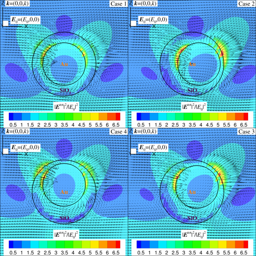
(a) (a)

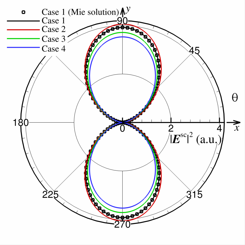
(b) (b)

Figure 1: (a) The total electric field vectors and contour plots of $|\boldsymbol{E}^{\mathrm{tot}}|^{2}/|E_{0}|^{2}$ in the $y=0$ plane are shown for four cases when the center of the core is (1) concentric with the shell, (2) shifted by $(20\,\mathrm{nm})\boldsymbol{e}_{x}$, (3) shifted by $(14.14\,\mathrm{nm})\boldsymbol{e}_{x}+(14.14\,\mathrm{nm})\boldsymbol{e}_{z}$, and (4) shifted by $(20\,\mathrm{nm})\boldsymbol{e}_{z}$. (b) The angular scattering intensity for the above four cases in the $z=0$ plane is shown. For the concentric case, the corresponding Mie series solution is also shown for comparison. (Cases 2 and 3 are shown in Visualization 1.)

We illustrate the developed framework with several carefully chosen examples that show the interaction between different types of scatterers and the incident wave. These examples are:

1. Scattering by an $\mathrm{Au}$ nano-sphere located at different positions inside a $\mathrm{SiO}_{2}$ shell whose size is comparable to the wavelength of the incident wave, i.e., when the wavenumber $k$ times the characteristic size $a$ of the scatterer is of order one, $ka\sim O(1)$. The numerical procedure for this core-shell particle case is slightly more complicated due to the presence of multiple domains. When $\boldsymbol{r}_{0}$ is located on $S_{\text{SiO}_{2}}$, the $\Sigma$ in (9) for the exterior domain is $\Sigma=S_{\text{SiO}_{2}}+S_{\infty}$ and $\Sigma=S_{\text{SiO}_{2}}+S_{\text{Au}}$ for the interior domain. When $\boldsymbol{r}_{0}$ is located on $S_{\text{Au}}$, the $\Sigma$ in (9) for the exterior domain is $\Sigma=S_{\text{SiO}_{2}}+S_{\text{Au}}$ and $\Sigma=S_{\text{Au}}$ for the interior domain. This example illustrates the Mie scattering regime (optical wave phenomena) and is of interest, for example, in light absorption enhancement applications for thin film solar cells [18];

2. Scattering of visible light by two $\mathrm{Au}$ nano-particles with different shapes but having the same volume. This example shows how the shape can be used to tune the resonance wavelength and the absorption cross-section when the characteristic length of the particle is much smaller than the wavelength of the incident wave. This scattering example is in the Rayleigh scattering regime and such quasi-electrostatic scattering problems are often encountered in micro- and nano- photonics;

3. Scattering by a dielectric oblate spheroid where the scatterer acts as a lens. In this example, the dimension of the spheroid (lens) is larger than the incident wavelength, and thus this example is approaching the geometrical optics regime.

In all these examples, the incident wave is plane wave given by $\boldsymbol{E}^{\mathrm{inc}}=E_{0}\exp{(\mathrm{i}kz)}\boldsymbol{e}_{x}$.

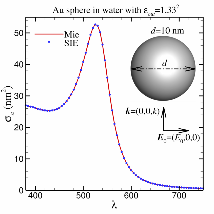
(a) (a)

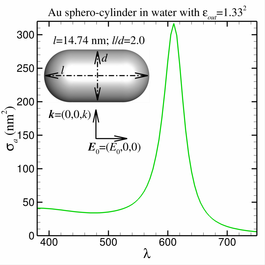
(b) (b)

Figure 2: Absorption cross-section of (a) $\mathrm{Au}$ sphere and (b) $\mathrm{Au}$ sphero-cylinder (cylinder with rounded spherical sides) is shown. In (a), the continuous line is obtained from the Mie series solution while the symbols are calculated via our field-only nonsingular surface integral method. In (b), the volume of the sphero-cylinder particle is the same as the volume of the sphere in (a).

3.1 Mie Scattering Example

The scattering of a plane wave by a particle in air consisting of a metal $\mathrm{Au}$ core of radius $60\,\mathrm{nm}$ embedded into a $\mathrm{SiO}_{2}$ shell of radius $90\,\mathrm{nm}$ is selected as an example for Mie scattering. We chose the size of the shell to be consistent with what is used in thin film solar cells to enhance light absorption [18]. Note that the core of the particle is not necessarily situated at the center of the shell. The total electric field vectors and the intensity contour plots are shown in Figure 1a for the incident wavelength of $520\,\mathrm{nm}$ (green light). In this example, the index of refraction of the $\mathrm{SiO}_{2}$ shell is $n_{\mathrm{SiO}_{2}}=1.47$ [19] and the index of refraction of the $\mathrm{Au}$ core is $n_{\mathrm{Au}}=0.65+2.02\mathrm{i}$ [20]. The plots in Figure 1a are shown in the $y=0$ plane with the center of the core (1) concentric with the shell, (2) shifted by $(20\,\mathrm{nm})\boldsymbol{e}_{x}$, (3) shifted by $(14.14\,\mathrm{nm})\boldsymbol{e}_{x}+(14.14\,\mathrm{nm})\boldsymbol{e}_{z}$, and (4) shifted by $(20\,\mathrm{nm})\boldsymbol{e}_{z}$.

From the electric field vector plots in Figure 1a, we see that the electric fields in the $\mathrm{Au}$ core are obviously out of phase to those in the $\mathrm{SiO}_{2}$ shell. The angular scattering intensities in the $z=0$ plane are shown for all four cases in Figure 1b. From Figure 1b, we also see that our numerical results agree very well with the Mie series solution [21, 22]. The maximum relative difference between the two solutions is less than than $0.6\%$.

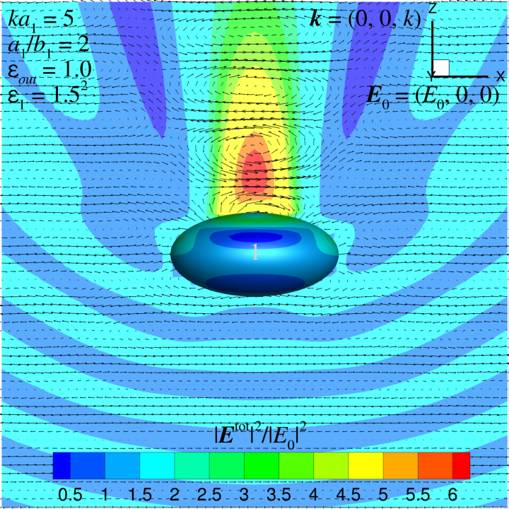
(a) (a)

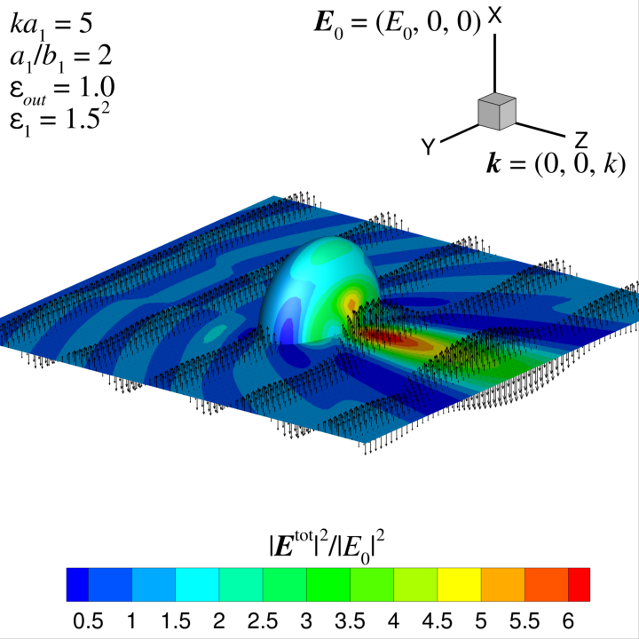
(b) (b)

Figure 3: Contour plots of $|\boldsymbol{E}^{\mathrm{tot}}|^{2}/|E_{0}|^{2}$ (a) in the $y=0$ plane, (b) in the $z=0$ plane, for a lens-shaped object approaching the geometrical optics regime. The instantaneous electric field vectors are also indicated. See also Visualization 2.

3.2 Rayleigh Scattering Example

In the previous example, we illustrated the ability and the accuracy of our field-only nonsingular surface integral method to solve scattering problems in the Mie scattering regime, $ka\sim O(1)$. When $ka$ is close to zero, that is, within the quasi-electrostatic limit, the scattering problem enters the Rayleigh scattering regime. The Rayleigh scattering regime is widely observed in microphotonics and nanophotonics with broad applications such as sensing of chemical and biological species [23]. We present the effect of the scatterer’s shape at a fixed volume on the absorption cross-section $\sigma_{a}$ of an $\mathrm{Au}$ particle in water with the refractive index of $n_{\mathrm{H_{2}0}}=1.33$. The $\mathrm{Au}$ particle is illuminated by the plane wave of wavelength varying from $380\,\mathrm{nm}$ to $750\,\mathrm{nm}$ in steps of $5\,\mathrm{nm}$. The absorption cross-section is calculated from the time-average Poynting vector via

$$\sigma_{a}=\left(\frac{1}{I^{\mathrm{inc}}}\right)\frac{1}{2}\int[\boldsymbol{E}^{\mathrm{tot}}\times(\boldsymbol{H}^{\mathrm{tot}})^{*}]\cdot\mathrm{d}\boldsymbol{S},$$ (15)

where $I^{\mathrm{inc}}=(1/2)v_{p}\epsilon_{0}|{E}_{0}|^{2}$, $v_{p}$ is the speed of the electromagnetic wave in water, and ^∗ denotes the complex conjugate. From Figure 2a, we see that for the spherical $\mathrm{Au}$ particle of diameter $d=10\,\mathrm{nm}$, the resonant wavelength occurs at around 540 nm. The complex index of refraction on resonance is $n_{\mathrm{Au}}=0.48+2.23\mathrm{i}$ [20]. Once again, the results produced via our field-only nonsingular surface integral method and the Mie series [21, 22] are in excellent agreement. Note that, even though in this example the ratio $d/\lambda\ll 1$, our method is not affected by any zero-frequency numerical instability issues.

Consider next a nano sphero-cylinder $\mathrm{Au}$ particle with the same volume as the sphere above. The length of the sphero-cylinder is $l=14.74\,\mathrm{nm}$ and the aspect ratio between its length and width is $l/d=2$. From Figure 2b, we can see that when the long axis of the sphero-cylinder is orientated along the polarization direction of the incident wave, the resonance wavelength is red shifted to $610\,\mathrm{nm}$. The complex index of refraction on resonance is $n_{\mathrm{Au}}=0.22+3.02\mathrm{i}$ [20] and the peak absorption cross-section is enhanced almost 6-fold relative to the $\mathrm{Au}$ sphere with the same volume.

3.3 Nano Lens Example

In the previous two examples, we tested our method in the Mie and Rayleigh scattering regimes. We now turn our attention to the geometrical optics regime, where $ka>O(1)$. Consider a dielectric oblate spheroid $(x^{2}+y^{2})/a^{2}+z^{2}/b^{2}=1$ with aspect ratio of $a/b=2$ and length of $ka=5$. The spheroid is characterized by the index of refraction of $n_{\mathrm{in}}=1.5$ and is suspended in air with the short axis parallel to the polarization of the incident wave. From Figure 3, we see that the wave is focused after it passes through the oblate spheroid and thus indicating the focusing ability of the oblate spheroid that is similar to an optical lens. The values of the fields in Figure 3 were obtained via our method by first solving (12) and then using the method described by Sun et al.[17] to compute the field inside and outside of the oblate spheroid. Note that the accuracy of this method is not affected by the near singular nature of the kernels when the observation point is near the boundary. If we were to use a conventional approach with its near singular Green’s function based kernels, then obtaining these values would have been numerically challenging.

4 Conclusions

The electric field on, near, inside and far away from a dielectric scatterer can be obtained easily with the proposed surface integral method. The solution satisfies both the vector Helmholtz equation and the divergence-free constraint inside and outside the scatterer. The accuracy of the solution is improved by employing a fully desingularized surface integral method.

Some typical numerical examples were chosen representative of nano and micro optical systems. A dielectric scattering sphere was extensively tested and compared against classical Mie theory and a (nano) lens was also considered.

In our previous publication on scattering from PEC bodies [14], we listed a number of advantages of our surface integral method over the most popular methods based on the Stratton–Chu[5, 4] or the PMCHWT[6, 7, 8] formulation. In this paper, we have shown that these advantages carry over to the dielectric case. For completeness and ease of reference we list these advantages here once more; namely,

1. Our method is conceptually simple and numerically straightforward because it focuses on solving directly for physically important quantities, namely, the electric field and its normal derivative on the surface of the scatterer. One of most obvious application of this method is its usefulness in computing the optical force on the dialectic particles;

2. Our method does not need to work with intermediate quantities such as surface currents. As such, elaborate vector basis functions (such as RWG [24, 25]) are not required and the standard boundary element techniques can be employed. Furthermore, our method only requires a boundary element solver for the scalar Helmholtz equation;

3. The robust, effective and accurate nonsingular surface integral method [26, 17] (also see Appendix B) that is based on nonsingular integrands and uses quadratic surface elements provides a more precise representation of the boundary geometry;

4. Our method may be advantageous in solving time-domain scattering problems using inverse Fourier transforms [27] because it directly solves for the electric field;

5. The framework presented here is not affected by certain numerical issues encountered in other implementations. For example, there are no integrals with strong singularities [28] and the zero frequency catastrophe [9, 29] is avoided altogether.

Given the symmetry between the $\boldsymbol{E}$ field and the $\boldsymbol{H}$ field, our theoretical framework can also be used to solve for the $\boldsymbol{H}$ field. One only needs to replace $\boldsymbol{E}$ by $\boldsymbol{H}$, $\boldsymbol{H}$ by $-\boldsymbol{E}$, and interchange $\epsilon$ with $\mu$ in the formulas given above.

Appendix A Continuity of H-Field on the Interface

The tangential component of $\boldsymbol{H}$ in the $\boldsymbol{t}_{1}$-direction can be expressed as $H_{t_{1}}=\boldsymbol{t}_{1}\cdot(\boldsymbol{n}\times\boldsymbol{H})$. The magnetic field can be expressed in terms of the electric field via $(\omega\mu)\boldsymbol{H}=-\mathrm{i}\boldsymbol{\nabla}\times\boldsymbol{E}$. Thus, for the tangential component of the magnetic field we have

$$\left(\frac{\omega\mu}{\mathrm{i}}\right)H_{t_{1}}=-\boldsymbol{t}_{1}\cdot(\boldsymbol{n}\times\boldsymbol{\nabla}\times\boldsymbol{E})=\boldsymbol{t}_{1}\cdot\frac{\partial\boldsymbol{E}}{\partial n}-\boldsymbol{n}\cdot\frac{\partial\boldsymbol{E}}{\partial t_{1}}.$$ (A1)

Writing $\partial\boldsymbol{E}/\partial t_{1}$ as

$$\frac{\partial\boldsymbol{E}}{\partial t_{1}}\equiv \frac{\partial(E_{n}\boldsymbol{n}+E_{t_{1}}\boldsymbol{t}_{1}+E_{t_{2}}\boldsymbol{t}_{2})}{\partial t_{1}}$$

$$= \quad\boldsymbol{n}\frac{\partial E_{n}}{\partial t_{1}}+E_{n}\frac{\partial\boldsymbol{n}}{\partial t_{1}}+\boldsymbol{t}_{1}\frac{\partial E_{t_{1}}}{\partial t_{1}}+E_{t_{1}}\frac{\partial\boldsymbol{t}_{1}}{\partial t_{1}}+\boldsymbol{t}_{2}\frac{\partial E_{t_{2}}}{\partial t_{1}}+E_{t_{2}}\frac{\partial\boldsymbol{t}_{2}}{\partial t_{1}}$$

using $\partial\boldsymbol{n}/\partial t_{1}=-\kappa_{1}\boldsymbol{t}_{1}$ and $\partial\boldsymbol{t}_{1}/\partial t_{1}=\kappa_{1}\boldsymbol{n}$, with $\kappa_{1}$ the curvature in the $t_{1}$ direction (see identities (A9)–(A11) in [14]) yields

$$\boldsymbol{n}\cdot\frac{\partial\boldsymbol{E}}{\partial t_{1}}=\frac{\partial E_{n}}{\partial t_{1}}+\kappa_{1}E_{t_{1}}.$$ (A2)

Applying (7b) and (A1) to the incident, scattered, and transmitted fields yields

$$\frac{1}{\mu_{\mathrm{out}}}\left[\boldsymbol{t}_{1}\cdot\frac{\partial(\boldsymbol{E}^{\mathrm{inc}}+\boldsymbol{E}^{\mathrm{sc}})}{\partial n}-\boldsymbol{n}\cdot\frac{\partial(\boldsymbol{E}^{\mathrm{inc}}+\boldsymbol{E}^{\mathrm{sc}})}{\partial t_{1}}\right]$$ (A3)

$$= \frac{1}{\mu_{\mathrm{in}}}\left[\boldsymbol{t}_{1}\cdot\frac{\partial\boldsymbol{E}^{\mathrm{tr}}}{\partial n}-\boldsymbol{n}\cdot\frac{\partial\boldsymbol{E}^{\mathrm{tr}}}{\partial t_{1}}\right]$$

and, after using (A2), we obtain the desired result (7c). A similar derivation can be done for the tangential component in the $\boldsymbol{t}_{2}$-direction.

Appendix B Nonsingular Surface Integral Equation

A brief description of the nonsingular surface integral method to solve the scalar Helmholtz equation is now presented. Take a scalar function $p(\boldsymbol{r})$ that satisfies the 3D Helmholtz equation $\nabla^{2}p(\boldsymbol{r})+k^{2}p(\boldsymbol{r})=0$, where, for example, $p$ represents one of the Cartesian components of the electric field. The nonsingular surface integral equation is given by [26]

$$\int_{S}{\Big{[}p(\boldsymbol{r})-p(\boldsymbol{r}_{0})g(\boldsymbol{r})-\frac{\partial{p(\boldsymbol{r}_{0})}}{{\partial{n}}}f(\boldsymbol{r})\Big{]}\frac{\partial{G}}{{\partial{n}}}\,\mathrm{d}S(\boldsymbol{r}})=$$

$$\int_{S}{\Big{[}\frac{\partial{p(\boldsymbol{r})}}{{\partial{n}}}-p(\boldsymbol{r}_{0})\frac{\partial{g(\boldsymbol{r})}}{{\partial{n}}}-\frac{\partial{p(\boldsymbol{r}_{0})}}{{\partial{n}}}\frac{\partial{f(\boldsymbol{r})}}{{\partial{n}}}\Big{]}G\,\mathrm{d}S(\boldsymbol{r}}),$$ (B1)

where $\boldsymbol{r}$ is the source point and $\boldsymbol{r}_{0}$ is the field (observation) point. The functions $f(\boldsymbol{r})$ and $g(\boldsymbol{r})$ in (Appendix B) must satisfy the Helmholtz equation and also satisfy the following conditions at $\boldsymbol{r}=\boldsymbol{r}_{0}$:

$$f(\boldsymbol{r}_{0}) = 0,\qquad\boldsymbol{n}(\boldsymbol{r}_{0})\cdot\boldsymbol{\nabla}f(\boldsymbol{r}_{0})=1,$$ (B2a)

$$g(\boldsymbol{r}_{0}) = 1,\qquad\boldsymbol{n}(\boldsymbol{r}_{0})\cdot\boldsymbol{\nabla}g(\boldsymbol{r}_{0})=0.$$ (B2b)

The functions $f(\boldsymbol{r})$ and $g(\boldsymbol{r})$ are not uniquely determined, see Klaseboer et al. [26] and Sun et al. [17] for more details. Note that the solid angle will be eliminated using this framework. In this paper, we used two standing wave functions for $f$ and $g$, i.e.,

$$f(\boldsymbol{r}) = \displaystyle{\frac{1}{k}}\sin\big{(}k\boldsymbol{n}(\boldsymbol{r}_{0})\cdot[\boldsymbol{r}-\boldsymbol{r}_{0}]\big{)},$$ (B3a)

$$g(\boldsymbol{r}) = \cos\big{(}k\boldsymbol{n}(\boldsymbol{r}_{0})\cdot[\boldsymbol{r}-\boldsymbol{r}_{0}]\big{)}.$$ (B3b)

If the Helmholtz equation is solved in the domain exterior to the scatterer, an additional factor $4\pi p(\boldsymbol{r}_{0})$ must be added to the left hand side of (Appendix B) due to the particular choice we made in (B3). This contribution results from evaluating (Appendix B) over a fictitious surface at infinity and depends on the choice of $f$ and $g$. Equation (Appendix B) is essentially the standard boundary element method implementation, where a known analytic solution $p(\boldsymbol{r}_{0})g(\boldsymbol{r})+[\partial p(\boldsymbol{r}_{0})/\partial n]f(\boldsymbol{r})$ has been subtracted. In this context, $p(\boldsymbol{r}_{0})$ and $\partial p(\boldsymbol{r}_{0})/\partial n$ are constants (for one particular node $\boldsymbol{r}_{0}$). This framework has been extensively tested for the Helmholtz equation in sound waves [17], electromagnetic scattering [13], and even elastic waves in solids [30]. Due to the fact that the formulation is nonsingular, Gaussian quadrature can be used on all elements (including the previous singular ones) and the implementation of higher order elements is straightforward.

Although the desingularized surface integral framework is not essential to solve the considered electromagnetic scattering problem, it does greatly improve the ease of implementation of the matrix systems $\cal{G}$ and $\cal{H}$, see (10) and Appendix B in [14], and it also improves the accuracy of the solution.

Appendix C Partial Derivatives Matrix

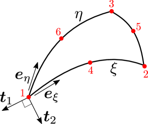
Figure 4: A quadratic surface patch with six nodes is shown.

The tangential derivatives, $\partial/\partial t_{1}$ and $\partial/\partial t_{2}$, can be obtained from the directional derivatives. Suppose that the tangential derivatives are sought at node $1$ of the six-noded quadratic surface element shown in Figure 4. Assume that the side 1-4-2 is represented by $\xi$ and the side 1-6-3 by $\eta$. Unit vectors in these two directions are denoted by $\boldsymbol{e}_{\xi}$ and $\boldsymbol{e}_{\eta}$, respectively. While $\boldsymbol{t}_{1}$ and $\boldsymbol{t}_{2}$ are perpendicular to each other, in general, $\boldsymbol{e}_{\xi}$ and $\boldsymbol{e}_{\eta}$ are not. The directional derivative in the $\xi$-direction can be written as

$$D_{\xi}f =\boldsymbol{e}_{\xi}\cdot\boldsymbol{\nabla}f=\boldsymbol{e}_{\xi}\cdot\left[\boldsymbol{t}_{1}\frac{\partial f}{\partial t_{1}}+\boldsymbol{t}_{2}\frac{\partial f}{\partial t_{2}}+\boldsymbol{n}\frac{\partial f}{\partial n}\right]$$

$$\approx\frac{f_{4}-f_{1}}{l_{41}},$$ (C1)

where $l_{41}$ denotes the Euclidean distance between nodes $1$ and $4$. Note that to obtain (C1), we used a simple numerical approximation to the directional derivative. Similarly, for the $\eta$-direction we use nodes $6$ and $1$ to obtain

$$D_{\eta}f=(\boldsymbol{e}_{\eta}\cdot\boldsymbol{t}_{1})\frac{\partial f}{\partial t_{1}}+(\boldsymbol{e}_{\eta}\cdot\boldsymbol{t}_{2})\frac{\partial f}{\partial t_{2}}\approx\frac{f_{6}-f_{1}}{l_{61}}.$$ (C2)

Solving (C1) and (C2) yields

$$\frac{\partial f}{\partial t_{1}} =\frac{1}{D}\left[(\boldsymbol{e}_{\xi}\cdot\boldsymbol{t}_{2})\frac{f_{6}-f_{1}}{l_{61}}-(\boldsymbol{e}_{\eta}\cdot\boldsymbol{t}_{2})\frac{f_{4}-f_{1}}{l_{41}}\right]$$ (C3a)

and

$$\frac{\partial f}{\partial t_{2}} =\frac{1}{D}\left[(\boldsymbol{e}_{\eta}\cdot\boldsymbol{t}_{1})\frac{f_{4}-f_{1}}{l_{41}}-(\boldsymbol{e}_{\xi}\cdot\boldsymbol{t}_{1})\frac{f_{6}-f_{1}}{l_{61}}\right],$$ (C3b)

where the determinant $D=(\boldsymbol{e}_{\xi}\cdot\boldsymbol{t}_{2})(\boldsymbol{e}_{\eta}\cdot\boldsymbol{t}_{1})-(\boldsymbol{e}_{\xi}\cdot\boldsymbol{t}_{1})(\boldsymbol{e}_{\eta}\cdot\boldsymbol{t}_{2})$. Notice that (C3) expresses $\partial f/\partial t_{1}$ and $\partial f/\partial t_{2}$ in terms of the values at the nodes . The simplest possible implementation is shown above, but a more accurate quadratic scheme can be obtained by using nodes 1, 4 and 2 in the numerical derivatives for $\xi$. As a further improvement, the above scheme has been applied to all elements surrounding node 1 and was averaged by the number of surrounding elements. The implementation for other nodes is very similar. In the numerical implementation, $f$ is the unknown variable $E_{n}^{\mathrm{sc}}$ and thus, $\partial/\partial t_{1}$ and $\partial/\partial t_{2}$ become $N\times N$ matrices, which have to be multiplied with the matrix $t_{1\alpha}{\cal{G}}_{\mathrm{in}}$ to contribute to the terms $\bar{{\cal{H}}}^{n\alpha}_{\mathrm{in}}$ in (12).

The matrices representing $\partial/\partial t_{1}$ and $\partial/\partial t_{2}$ can also elegantly be employed to calculate the curvatures $\kappa_{1}$ and $\kappa_{2}$ via (see (A9c) and (A9d) in [14])

$$\kappa_{1}=-\boldsymbol{t}_{1}\cdot\frac{\partial\boldsymbol{n}}{\partial t_{1}}\quad\text{and}\quad\kappa_{2}=-\boldsymbol{t}_{2}\cdot\frac{\partial\boldsymbol{n}}{\partial t_{2}}.$$ (C4)

Appendix D Linear Matrix System

We now demonstrate how to assemble the linear matrix system of equations in terms of the interior field $\boldsymbol{E}^{\mathrm{tr}}$ and $\partial\boldsymbol{E}^{\mathrm{tr}}/\partial n$ following the same procedure given in Section 2.

To write $\boldsymbol{n}\cdot\partial\boldsymbol{E}^{\mathrm{sc}}/\partial n$ in terms of $\boldsymbol{E}^{\mathrm{tr}}$ and $\partial\boldsymbol{E}^{\mathrm{tr}}/\partial n$, we can rearrange (7a), and after using (6a), we have

$$\boldsymbol{n}\cdot\frac{\partial{\boldsymbol{E}^{\mathrm{sc}}}}{\partial{n}}=\kappa(\epsilon_{\mathrm{io}}-1)E^{\mathrm{tr}}_{n}+\boldsymbol{n}\cdot\frac{\partial{\boldsymbol{E}^{\mathrm{tr}}}}{\partial{n}}-\boldsymbol{n}\cdot\frac{\partial{\boldsymbol{E}^{\mathrm{inc}}}}{\partial{n}}\qquad\text{where}\qquad\epsilon_{\mathrm{io}}\equiv\epsilon_{\mathrm{in}}/\epsilon_{\mathrm{out}}.$$ (D1)

To write $\{\boldsymbol{t}_{1}\cdot\partial\boldsymbol{E}^{\mathrm{sc}}/\partial n,\,\boldsymbol{t}_{2}\cdot\partial\boldsymbol{E}^{\mathrm{sc}}/\partial n\}$ in terms of $\boldsymbol{E}^{\mathrm{tr}}$ and $\partial\boldsymbol{E}^{\mathrm{tr}}/\partial n$ we express the continuity of the tangential components of $\boldsymbol{H}$ on $S$ given by (7b) in terms of the electric field with $\mu_{\mathrm{oi}}\equiv\mu_{\mathrm{out}}/\mu_{\mathrm{in}}$ and $j=1,2$ (see Appendix A for details):

$$\left(\epsilon_{\mathrm{io}}-\mu_{\mathrm{oi}}\right)\frac{\partial}{\partial t_{j}}E_{n}^{\mathrm{tr}}+\kappa_{j}\left(1-\mu_{\mathrm{oi}}\right)E_{t_{j}}^{\mathrm{tr}}-\boldsymbol{t}_{j}\cdot\frac{\partial\boldsymbol{E}^{\mathrm{inc}}}{\partial n}+\mu_{\mathrm{oi}}\boldsymbol{t}_{j}\cdot\frac{\partial\boldsymbol{E}^{\mathrm{tr}}}{\partial n}=\boldsymbol{t}_{j}\cdot\frac{\partial\boldsymbol{E}^{\mathrm{sc}}}{\partial n}.$$ (D2)

As such, the linear system in terms of $\boldsymbol{E}^{\mathrm{tr}}$ and $\partial\boldsymbol{E}^{\mathrm{tr}}/\partial n$ can be found to be

$$\begin{bmatrix}\bar{{\cal{H}}}^{nx}&\bar{{\cal{H}}}^{t1x}&\bar{{\cal{H}}}^{t2x}&-{n_{x}}{\cal{G}}&-\mu_{\mathrm{oi}}{t_{1x}}{\cal{G}}&-\mu_{\mathrm{oi}}{t_{2x}}{\cal{G}}\\ \bar{{\cal{H}}}^{ny}&\bar{{\cal{H}}}^{t1y}&\bar{{\cal{H}}}^{t2y}&-{n_{y}}{\cal{G}}&-\mu_{\mathrm{oi}}{t_{1y}}{\cal{G}}&-\mu_{\mathrm{oi}}{t_{2y}}{\cal{G}}\\ \bar{{\cal{H}}}^{nz}&\bar{{\cal{H}}}^{t1z}&\bar{{\cal{H}}}^{t2z}&-{n_{z}}{\cal{G}}&-\mu_{\mathrm{oi}}{t_{1z}}{\cal{G}}&-\mu_{\mathrm{oi}}{t_{2z}}{\cal{G}}\\ n_{x}{\cal{H}}_{\mathrm{in}}&t_{1x}{\cal{H}}_{\mathrm{in}}&t_{2x}{\cal{H}}_{\mathrm{in}}&-n_{x}{\cal{G}}_{\mathrm{in}}&-t_{1x}{\cal{G}}_{\mathrm{in}}&-t_{2x}{\cal{G}}_{\mathrm{in}}\\ n_{y}{\cal{H}}_{\mathrm{in}}&t_{1y}{\cal{H}}_{\mathrm{in}}&t_{2y}{\cal{H}}_{\mathrm{in}}&-n_{y}{\cal{G}}_{\mathrm{in}}&-t_{1y}{\cal{G}}_{\mathrm{in}}&-t_{2y}{\cal{G}}_{\mathrm{in}}\\ n_{z}{\cal{H}}_{\mathrm{in}}&t_{1z}{\cal{H}}_{\mathrm{in}}&t_{2z}{\cal{H}}_{\mathrm{in}}&-n_{z}{\cal{G}}_{\mathrm{in}}&-t_{1z}{\cal{G}}_{\mathrm{in}}&-t_{2z}{\cal{G}}_{\mathrm{in}}\end{bmatrix}\begin{bmatrix}E_{n}^{\mathrm{tr}}\\ E_{t_{1}}^{\mathrm{tr}}\\ E_{t_{2}}^{\mathrm{tr}}\\ \boldsymbol{n}\cdot\frac{\partial\boldsymbol{E}^{\mathrm{tr}}}{\partial n}\\ \boldsymbol{t}_{1}\cdot\frac{\partial\boldsymbol{E}^{\mathrm{tr}}}{\partial n}\\ \boldsymbol{t}_{2}\cdot\frac{\partial\boldsymbol{E}^{\mathrm{tr}}}{\partial n}\end{bmatrix}=\begin{bmatrix}{\cal{A}}_{x}\\ {\cal{A}}_{y}\\ {\cal{A}}_{z}\\ 0\\ 0\\ 0\end{bmatrix},$$ (D3a)

where

$$\bar{{\cal{H}}}^{n\alpha} =\epsilon_{\mathrm{io}}n_{\alpha}{\cal{H}}-\kappa\left(\epsilon_{\mathrm{io}}-1\right)n_{\alpha}{\cal{G}}-(\epsilon_{\mathrm{io}}-\mu_{\mathrm{oi}})t_{1\alpha}{\cal{G}}\frac{\partial}{\partial t_{1}}-(\epsilon_{\mathrm{io}}-\mu_{\mathrm{oi}})t_{2\alpha}{\cal{G}}\frac{\partial}{\partial t_{2}},$$ (D3b)

$$\bar{{\cal{H}}}^{t1\alpha} =t_{1\alpha}{\cal{H}}-\kappa_{1}(1-\mu_{\mathrm{oi}})t_{1\alpha}{\cal{G}}\quad\text{and}\quad\bar{{\cal{H}}}^{t2\alpha}=t_{2\alpha}{\cal{H}}-\kappa_{2}(1-\mu_{\mathrm{oi}})t_{2\alpha}{\cal{G}},$$ (D3c)

and

$${\cal{A}}_{\alpha}= \;\;\;{\cal{H}}\left[n_{\alpha}E_{n}^{\mathrm{inc}}+t_{1\alpha}E^{\mathrm{inc}}_{t_{1}}+t_{2\alpha}E^{\mathrm{inc}}_{t_{2}}\right]$$

$$-{\cal{G}}\left[n_{\alpha}\boldsymbol{n}\cdot\frac{\partial\boldsymbol{E}^{\mathrm{inc}}}{\partial n}+t_{1\alpha}\boldsymbol{t}_{1}\cdot\frac{\partial\boldsymbol{E}^{\mathrm{inc}}}{\partial n}+t_{2\alpha}\boldsymbol{t}_{2}\cdot\frac{\partial\boldsymbol{E}^{\mathrm{inc}}}{\partial n}\right]$$ (D3d)

with $$\alpha=x,y,z.$$

Funding

Australian Research Council (ARC) (DE150100169, CE140100003, DP170100376).
This work was partially supported by U.S. government, not protected by U.S. copyright.

Disclosures

The authors declare that there are no conflicts of interest related to this article.

References

- [1] F. Frezza, F. Mangini, and N. Tedeschi, “Introduction to electromagnetic scattering: tutorial,” \JournalTitleJournal of the Optical Society of America A 35, 163–173 (2018).
- [2] A. J. Yuffa and J. Markkanen, “A 3-D tensorial integral formulation of scattering containing intriguing relations,” \JournalTitleIEEE Transactions on Antennas and Propagation 66, 5274–5281 (2018).
- [3] E. Klaseboer, Q. Sun, and D. Y. C. Chan, “Nonsingular field-only surface integral equations for electromagnetic scattering,” \JournalTitleIEEE Transactions on Antennas and Propagation 65, 972–977 (2017).
- [4] J. A. Stratton and L. J. Chu, “Diffraction theory of electromagnetic waves,” \JournalTitlePhys. Rev. 56, 99–107 (1939).
- [5] J. A. Stratton, Electromagnetic Theory (McGraw Hill, New York, 1941). Sec. 8.14.
- [6] A. J. Poggio and E. K. Miller, “Integral equation solutions of three-dimensional scattering problems,” in Computer Techniques for Electromagnetics, vol. 7 R. Mittra, ed. (Pergamon Press, Oxford, 1973).
- [7] T.-K. Wu and L. L. Tsai, “Scattering from arbitrarily-shaped lossy dielectric bodies of revolution,” \JournalTitleRadio Science 12, 709–718 (1977).
- [8] Y. Chang and R. Harrington, “A surface formulation for characteristic modes of material bodies,” \JournalTitleIEEE Transactions on Antennas and Propagation 25, 789–795 (1977).
- [9] F. Vico, M. Ferrando, L. Greengard, and Z. Gimbutas, “The decoupled potential integral equation for time-harmonic electromagnetic scattering,” \JournalTitleCommun. Pure Appl. Math. 69, 771–812 (2015).
- [10] X. Fu, J. Li, L. J. Jiang, and B. Shanker, “Generalized Debye sources-based EFIE solver on subdivision surfaces,” \JournalTitleIEEE Transactions on Antennas and Propagation 65, 5376–5386 (2017).
- [11] J. A. DeSanto, “A new formulation of electromagnetic scattering from rough dielectric interfaces,” \JournalTitleJournal of Electromagnetic Waves and Applications 7, 1293–1306 (1993).
- [12] J. DeSanto and A. Yuffa, “A new integral equation method for direct electromagnetic scattering in homogeneous media and its numerical confirmation,” \JournalTitleWaves in Random and Complex Media 16, 397–408 (2006).
- [13] Q. Sun, E. Klaseboer, and D. Y. C. Chan, “Robust multiscale field-only formulation of electromagnetic scattering,” \JournalTitlePhys. Rev. B 95, 045137 (2017).
- [14] Q. Sun, E. Klaseboer, A. J. Yuffa, and D. Y. C. Chan, “Robust field-only surface integral equations: Scattering from a perfect electric conductor,” \JournalTitleJ. Opt. Soc. Am. A (2019, submitted).
- [15] D. Colton and R. Kress, Integral Equation Methods in Scattering Theory (Krieger Publishing Company, 1992). Ch. 4.
- [16] J. Markkanen, A. J. Yuffa, and J. A. Gordon, “Numerical validation of a boundary element method with electric field and its normal derivative as the boundary unknowns,” \JournalTitleAppl. Comput. Electromagn. Soc. J. 34, 220–223 (2019).
- [17] Q. Sun, E. Klaseboer, B.-C. Khoo, and D. Y. C. Chan, “Boundary regularized integral equation formulation of the Helmholtz equation in acoustics,” \JournalTitleR. Soc. Open Sci. 2, 140520 (2015).
- [18] P. Yu, Y. Yao, J. Wu, X. Niu, A. L. Rogach, and Z. Wang, “Effects of plasmonic metal core-dielectric shell nanoparticles on the broadband light absorption enhancement in thin film solar cells,” \JournalTitleScientific Reports 7 (2017).
- [19] L. V. Rodríguez-de Marcos, J. I. Larruquert, J. A. Méndez, and J. A. Aznárez, “Self-consistent optical constants of and films,” \JournalTitleOptical Materials Express 6, 3622–3637 (2016).
- [20] A. D. Rakić, A. B. Djurišić, J. M. Elazar, and M. L. Majewski, “Optical properties of metallic films for vertical-cavity optoelectronic devices,” \JournalTitleApplied Optics 37, 5271–5283 (1998).
- [21] G. Mie, “Beiträge zur Optik trüber Medien, speziell kolloidaler Metallösungen,” \JournalTitleAnnalen der Physik 330, 377–445 (1908).
- [22] C. F. Bohren and D. R. Huffman, Absorption and scattering of light by small particles (John Wiley & Sons, New York, 1983).
- [23] K. M. Mayer and J. H. Hafner, “Localized surface plasmon resonance sensors,” \JournalTitleChemical Reviews 111, 3828–3857 (2011).
- [24] S. Belez, C. Bourlier, and G. Kubické, “Efficient propagation-inside-layer expansion algorithm for solving the scattering from three-dimensional nested homogeneous dielectric bodies with arbitrary shape,” \JournalTitleJournal of the Optical Society of America A 32, 392–401 (2015).
- [25] J. Li, D. Dault, N. Nair, and B. Shanker, “Analysis of scattering from complex dielectric objects using the generalized method of moments,” \JournalTitleJournal of the Optical Society of America A 31, 2346–2355 (2014).
- [26] E. Klaseboer, Q. Sun, and D. Y. C. Chan, “Non-singular boundary integral methods for fluid mechanics applications,” \JournalTitleJ. Fluid Mech. 696, 468–478 (2012).
- [27] E. Klaseboer, Q. Sun, and D. Y. C. Chan, “Field-only integral equation method for time domain scattering of electromagnetic pulses,” \JournalTitleApplied Optics 56, 9377 (2017).
- [28] W. C. Chew, “Some observations on the spatial and eigenfunction representations of dyadic Green’s functions (electromagnetic theory),” \JournalTitleIEEE Transactions on Antennas and Propagation 37, 1322–1327 (1989).
- [29] J.-S. Zhao and W. C. Chew, “Integral equation solution of Maxwell’s equations from zero frequency to microwave frequencies,” \JournalTitleIEEE Transactions on Antennas and Propagation 48, 1635–1645 (2000).
- [30] E. Klaseboer, Q. Sun, and D. Y. C. Chan, “Helmholtz decomposition and boundary element method applied to dynamic linear elastic problems,” \JournalTitleJournal of Elasticity (2018).