Parameter Estimation with a spinning multi-mode waveform model: IMRPhenomHM

Abstract

Gravitational waves from compact binary coalescence (CBC) sources can be decomposed into spherical-harmonic multipoles, the dominant being the quadrupole ( $(l,|m|)=(2,2)$ ) modes. The contribution of sub-dominant modes towards total signal power increases with increasing binary mass ratio and source inclination to the detector. It is well-known that in these cases neglecting higher modes could lead to measurement biases, but these have not yet been quantified with a higher-mode model that includes spin effects. In this study, we use the multi-mode aligned-spin phenomenological waveform model IMRPhenomHM London et al. (2018) to investigate the effects of including multi-mode content in estimating source parameters and contrast the results with using a quadrupole-only model (IMRPhenomD). We use as sources IMRPhenomHM and hybrid effective-one-body–numerical-relativity waveforms over a range of mass-ratio and inclination combinations, and recover the parameters with IMRPhenomHM and IMRPhenomD. These allow us to quantify the accuracy of parameter measurements using a multi-mode model, the biases incurred when using a quadrupole-only model to recover full (multi-mode) signals, and the systematic errors in the IMRPhenomHM model. We see that the parameters recovered by multi-mode templates are more precise for all non-zero inclinations as compared to quadrupole templates. For multi-mode injections, IMRPhenomD recovers biased parameters for non-zero inclinations with lower likelihood while IMRPhenomHM-recovered parameters are accurate for most cases, and if a bias exists, it can be explained as a combined effect of observational priors and (in the case of hybrid-NR signals) waveform inaccuracies. However, for cases where IMRPhenomHM recovers biased parameters, the bias is always significantly smaller than the corresponding IMRPhenomD recovery, and we conclude that IMRPhenomHM will be sufficiently accurate to allow unbiased measurements for most GW observations.

Introduction

The first gravitational-wave (GW) detection, from a binary black hole (BBH) merger, was achieved on the 14${}^{\text{th}}$ of September, 2015 Abbott et al. (2016) by the two Advanced LIGO (aLIGO) detectors at Hanford and Livingston Aasi et al. (2015). Two observing runs have since been completed by the aLIGO detectors, and from the second half of 2017, Advanced Virgo (AdV) Acernese et al. (2015) joined the GW detector network, facilitating the first three-detector observation of a BBH source Abbott et al. (2017a). During the first two observation runs of aLIGO and AdV, a total of ten binary black hole (BBH) mergers and one binary neutron star (BNS) merger were detected Abbott et al. (2018a, 2017b). Most signal measurements were performed using waveform models that included only the dominant quadrupole harmonic, although one signal (GW170729) showed evidence for a binary with unequal masses, for which models that include higher harmonics allow for improved measurements Chatziioannou et al. (2019). The goal of this work is to quantify the measurement accuracy possible with higher-multipole models.

Any GW $h(\theta,\phi,\vec{\lambda},t)$ can be decomposed in terms of spherical harmonics with spin-weight -2, ${}^{-2}Y_{lm}(\theta,\phi)$,

$$\leavevmode\nobreak\ h(\theta,\phi,\vec{\lambda},t)=\sum_{l}\sum_{m=-l}^{m=l}\ {}^{-2}Y_{lm}(\theta,\phi)h_{lm}(\vec{\lambda},t),$$ (1)

where $h_{lm}(\vec{\lambda},t)$ are the GW modes, and $\vec{\lambda}$ are the intrinsic parameters of the source, i.e., the black-hole masses and spins. For coalescing binary systems with aligned spins, or in the co-precessing frame of precessing systems Schmidt et al. (2011); O’Shaughnessy et al. (2011); Boyle et al. (2011), the quadrupole modes $(l,|m|)=(2,2)$ are the strongest. Relative to the corresponding quadrupole mode, the sub-dominant modes ($l=3,4,5\dots;|m|\in[0,l]\forall l$) are weakest for equal-mass systems, their strength increasing with increasing mass ratio. In addition, for a given system, as the binary’s inclination to the detector is increased from face-on $(\theta=0^{\circ})$ to edge-on $(\theta=90^{\circ})$, the contribution of the dominant modes decreases, as does the overall signal power, and the relative importance of sub-dominant modes grows.

Black-hole binaries in non-eccentric orbits are characterised by the two black-hole masses, $m_{1}$ and $m_{2}$, and the black-hole spins $\mathbf{S}_{1}$ and $\mathbf{S}_{2}$. The inspiral rate of the binary (and phasing of the GW signal, which is crucial to measuring the properties of the binary) is effected most strongly by combinations of these parameters: the chirp mass, $\mathcal{M}_{c}=(m_{1}m_{2})^{3/5}/(m_{1}+m_{2})^{1/5}$ (during the inspiral), and the total mass, $M=m_{1}+m_{2}$ (during the merger and ringdown); the mass ratio $q=m_{1}/m_{2}$, or alternatively symmetric mass ratio $\eta=m_{1}m_{2}/M^{2}$; and the weighted sum of the spin components parallel to the orbital angular momentum $\mathbf{\hat{L}}$, $\chi_{\rm eff}=(m_{1}\chi_{1}+m_{2}\chi_{2})/M$, where $\chi_{i}=\mathbf{S}_{i}\cdot\mathbf{\hat{L}}/m_{i}^{2}$ Poisson and Will (1995); Cutler and Flanagan (1994); Ajith et al. (2011); Baird et al. (2013). The overall strength of the GW signal scales with $M/d_{L}$, where $d_{L}$ is the distance from the source to the detector, and is also affected by the binary inclination $\theta_{\rm JN}$, which is the angle between the total angular momentum $\mathbf{\hat{J}}$ (or equivalently $\mathbf{\hat{L}}$ for aligned-spin binaries) and the line of sight, $\mathbf{\hat{N}}$. If there are spin components perpendicular to $\mathbf{\hat{L}}$, then the binary’s orbital plane and spins will precess, leading to modulations of the GW signal. In general, precession has little effect on the overall GW phase Buonanno et al. (2003); Schmidt et al. (2012), and so might not strongly effect the measurement of other parameters Brown et al. (2012); Fairhurst et al. (2019a). Precession has not yet been measured in GW observations Abbott et al. (2018a), and for these reasons we focus on aligned-spin binaries in this study, and expect that the general results will also hold for precessing systems.

Waveform models describing the inspiral-merger-ringdown (IMR) stages of BBH mergers are available for non-spinning, aligned-spin and precessing configurations. Many of the aligned-spin waveform models model only the dominant quadrupole mode, but several multi-mode models now exist. For non-spinning systems, there are effective-one-body (EOB)–numerical-relativity (NR) multi-mode models, EOBNRv2HM Pan et al. (2011) and TEOBiResumMultipoles Nagar et al. (2019), and “Phenom” models Mehta et al. (2017); Kumar Mehta et al. (2019). The EOBNR model was recently extended to aligned-spin systems (SEOBNRv4HM) Cotesta et al. (2018), and models the ($l,|m|$) = (2,2), (2,1), (3,3), (4,4) and (5,5) modes. In this study we will use the phenomenological aligned-spin multi-mode model IMRPhenomHM London et al. (2018), which models the $l=(2,3,4)$ & $|m|=(l,l-1)$ modes; IMRPhenomHM is described in more detail in Sec. I.1. Higher modes are also included in a series of surrogate models constructed from NR waveforms Blackman et al. (2015, 2017a, 2017b); Varma et al. (2019).

Previous studies have investigated the effect of employing higher-order mode models for gravitational wave searches Capano et al. (2014); Calderón Bustillo et al. (2017); Harry et al. (2018); Calderón Bustillo et al. (2018) and provided an estimate of the systematic errors that could be incurred from neglecting higher-order modes in the template waveforms Calderón Bustillo et al. (2016); Varma and Ajith (2017); Varma et al. (2014). In  Littenberg et al. (2013) and  Graff et al. (2015) the authors performed a full Bayesian analysis of the effects of including and neglecting higher-order modes in template waveforms non-spinning systems. We summarise some notable results relevant to the current study.

In Ref. Varma et al. (2014), the authors used multi-mode PN-NR hybrids as signals and computed the expected statistical and systematic errors from using quadrupole-only templates to estimate source parameters over a range of total mass and mass-ratio values, for a signal sky-averaged signal-to-noise ratio (SNR) of 8. The statistical errors are estimated from the Fisher Information Matrix, which is the noise-weighted inner product between partial derivatives of the waveform. The authors also estimate the systematic errors by calculating the fitting factor, which is the noise-weighted inner product between the signal and model waveforms, maximised over the model parameters. The effective systematic error is proportional to the difference between the best fit and true parameters. In this study, the authors found that non-inclusion of the subdominant modes in templates will lead to $\sim$10% loss in detection rate for $q\geq$6 and $M\geq 100M_{\odot}$ and will lead to systematic errors larger than statistical errors for $q\geq 4$ and $M\geq 150M_{\odot}$. The results obtained from a Fisher information matrix approximation are valid for high SNR events. To study the waveform errors for low or moderate SNRs and for a realistic assessment of the model’s measurement capabilities, a full Bayesian analysis is required.

In a Bayesian analysis, the physical parameters of the source are estimated by matching the detector data with model waveforms. Given detector data $d(t)$ and a waveform model $h(t)$, the posterior over $\vec{\lambda}$ is,

$$p(\vec{\lambda}|d(t),h(t,\vec{\lambda}))=\frac{p(\vec{\lambda}|h(t,\vec{\lambda}))p(d(t)|\vec{\lambda},h(t,\vec{\lambda}))}{p(d(t)|h(t,\vec{\lambda}))},$$ (2)

where $\vec{\lambda}$ is the vector of intrinsic and extrinsic parameters. $p(\vec{\lambda}|h(t,\vec{\lambda}))$, $p(d(t)|\vec{\lambda},h(t,\vec{\lambda}))$ and $p(d(t)|h(t,\vec{\lambda}))$ are the prior, likelihood and evidence respectively, where the likelihood is,

$$p(d(t)|\vec{\lambda},h(t,\vec{\lambda}))\propto e^{-\frac{1}{2}<d(t)-h(t,\vec{\lambda})|d(t)-h(t,\vec{\lambda})>},$$ (3)

and the quantity $<a|b>$ gives the noise-weighted inner product between the two functions; this is the match if $a$ and $b$ are descriptions of waveforms from systems with the same physical parameters, optimised over a relative time and phase shift. See Ref. Veitch et al. (2015) for more details on the techniques and algorithms employed for GW parameter estimation. Accuracy of the inferred parameters depends on the accuracy of the waveform model used to simulate the real signal and the noise content of the detector data.

In Ref. Littenberg et al. (2013), the authors injected multimode non-spinning NR waveforms in zero-noise at different mass ratios with fixed inclination of $60\degree$ and compared the systematic and statistical errors of the posteriors recovered by nonspinning quadrupole-only (EOBNRv2) and multi-mode (EOBNRv2HM) waveform models for non-spinning systems. They found that up to $q=6$ and for SNRs $\leq$ 50, the systematic errors from EOBNRv2HM were smaller than or comparable to the statistical errors. The fractional systematic error (defined as the ratio between systematic bias and statistical error) for the intrinsic parameters is consistently lower for EOBNRv2HM than EOBNRv2. Also, the posteriors were recovered at an overall higher likelihood by EOBNRv2HM than EOBNRv2 (see Fig. 2 of Ref. Littenberg et al. (2013)).

In Ref. Graff et al. (2015), the authors performed a comprehensive study of the effects of using EOBNRv2HM and EOBNRv2 templates to recover EOBNRv2HM signals across a range of total mass values ($50M_{\odot}\leq M_{total}\leq 500M_{\odot}$) and SNRs ($6\leq\rho\leq 18$) for $q=1.25$ and $q=4$ systems at two inclinations $(\theta_{JN}=0,60\degree)$. Consistent with Ref. Littenberg et al. (2013), the posteriors are recovered at an overall larger total evidence by EOBNRv2HM compared to EOBNRv2 for inclined systems; see Fig. 5 of Ref. Graff et al. (2015). These differences increase with increasing inclination, mass ratio and total mass. The posteriors are better constrained by the multi-mode model than a quadrupole-only model (see Fig. 7 of Ref. Graff et al. (2015)) with lower systematic bias for inclined systems. They found that the multi-mode model constrains the inclination angle better than quadrupole-only model, which in turn leads to better constraints on the distance.

In the previous studies, the authors used non-spinning multi-mode and quadrupole-only waveforms for the Bayesian analysis, and hence, were restricted in the ($m_{1}$, $m_{2}$) space for intrinsic parameters. In this study, we will use a multi-mode aligned-spin waveform template (IMRPhenomHM) and increase the dimensionality of the problem by one, i.e., covering the ($m_{1}$, $m_{2}$ and $\chi_{\rm eff}$) space of intrinsic parameters. Of course, the extrinsic parameter space remains the same.

One of the aims of this study is to explore the effects of using a multi-mode waveform template (IMRPhenomHM) on inferring source parameters from a multi-mode signal and to contrast it with a quadrupole-only model (IMRPhenomD). For this, we perform a set of injections at three different mass ratios and three inclinations in zero noise using the IMRPhenomHM model. This allows us to quantify parameter errors from not including sub-dominant modes in templates, and accuracy improvements when the sub-dominant modes are included.

IMRPhenomHM is an approximate model of the sub-dominant modes and does not model all of the higher harmonics (all modes with $l\geq 5$, all $m=0$ modes, and the (3,1), (4,2), (4,1) modes). The sub-dominant modes of the model are not tuned to NR simulations and mode-mixing effects are not modelled. With that in mind, the other aim of the study is to determine the ability of IMRPhenomHM to recover parameters of real physical signals. For that, we perform the same set of injections as for IMRPhenomHM injections but with multi-mode PN-NR hybrid waveforms and compare the parameters recovered by IMRPhenomD and IMRPhenomHM. Hybridisation is required to include the contributions to the signals below the starting frequency of the NR waveforms.

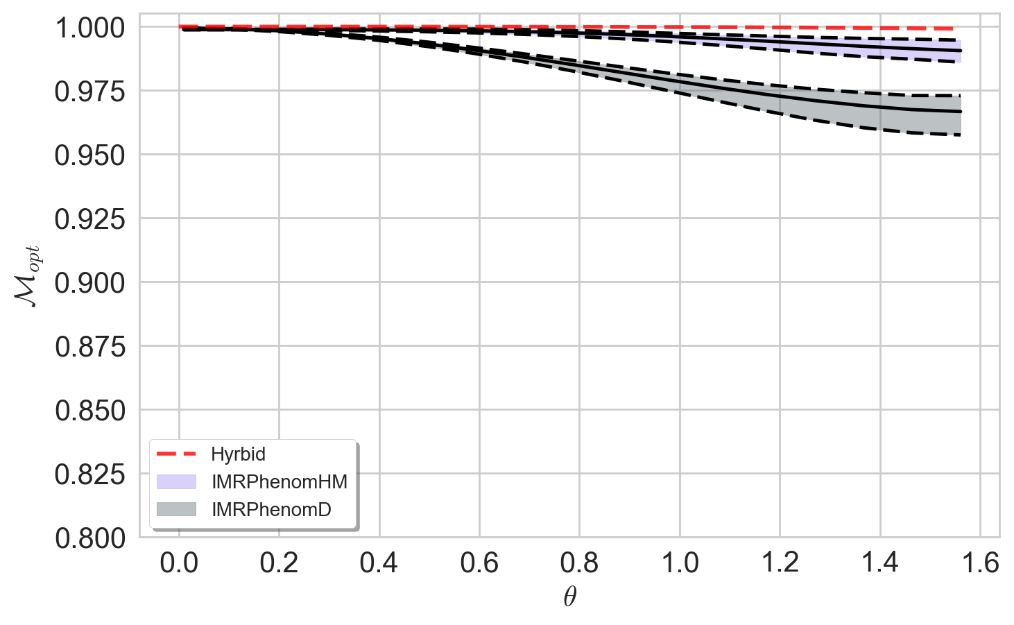
(a)

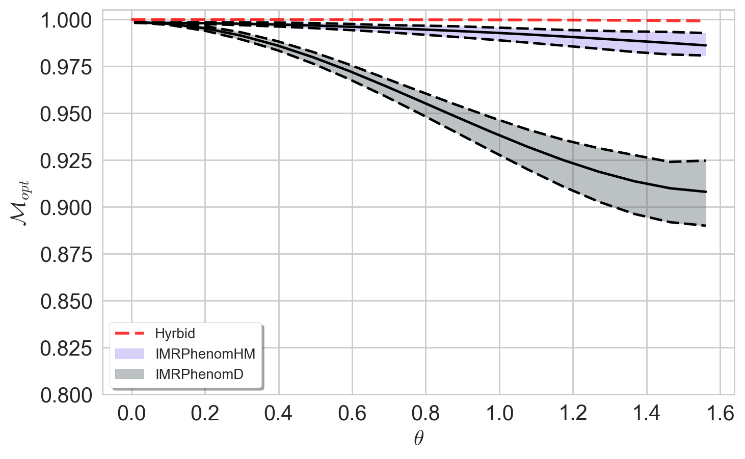
(b)

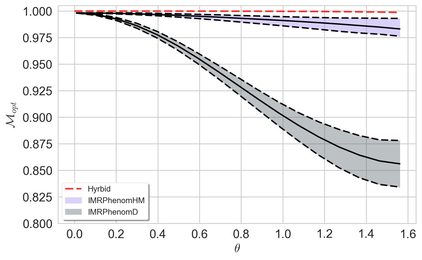
(c)

Figure 1: Match between Hybrid NR and IMRPhenomHM waveforms (blue) and IMRPhenomD waveforms (grey). The left, central and right panel gives matches for $q=(2,4,8)$ systems. The match is computed over a range of signal inclination, phase and polarisation values with the match optimized over template phase and polarisation. We quote the minimum (dashed-lower bound), average (central black line) and maximum value (dashed-upper bound) of the match at each signal inclination. The dashed red line shows the match between the multimode Hybrid-NR waveform and corresponding SXS waveform. For the match, the total mass is set to 100 M_⊙ with a lower-frequency bound of $f_{min}$ = 30Hz.

Sec. I will provide a short summary of the template waveform models IMRPhenomHM and IMRPhenomD  construction of the multi-mode hybrids and details of the setup for parameter estimation. The results will be introduced in general in Sec. II, and the specific results for intrinsic and extrinsic parameters will be given in Secs. III and IV.

I Methods

I.1 Summary of waveform models

IMRPhenomD Husa et al. (2016); Khan et al. (2016) is a quadrupole-only frequency-domain phenomenological waveform model describing inspiral-merger-ringdown (IMR) stages of aligned-spin BBH systems. IMRPhenomD is calibrated to NR simulations with $1\leq q\leq 18$ and spins $\left|\chi_{i}\right|\lesssim 0.85$. The agreement between IMRPhenomD and other quadrupole-only models is extremely good in the region of parameter space that we consider in this study Khan et al. (2016); Bohé et al. (2017), and so we expect that results obtained with this model will be indicative of the performance of any accurate quadrupole-only model.

IMRPhenomHM London et al. (2018) is a frequency domain aligned-spin phenomenological waveform model, wherein results from Post-Newtonian theory (for inspiral) and BH perturbation theory (for ringdown) are used to map the dominant quadrupole mode to the sub-dominant modes. So, given the quadrupole frequency ($f_{22}$), amplitude ($A_{22}$) and phase ($\varphi_{22}$), the frequency $(f_{lm})$, amplitude $(A_{lm})$ and phase $(\phi_{lm})$ of other modes are computed via,

$$\tilde{h}_{lm}(f) =A_{lm}(f)\times\exp\left\{i\,\varphi_{lm}(f)\right\}$$ (4)

$$\approx|\beta_{lm}(f)|\,A_{22}(f_{22}^{\rm A})\times\exp\left\{i\left[\kappa(f)\,\varphi_{22}(f_{22}^{\rm\varphi})+\Delta_{lm}(f)\right]\right\},$$ (5)

where $|\beta_{lm}(f)|$ and $\kappa(f)$ are amplitude and phase scaling functions and $\Delta_{lm}(f)$ are phase-shifts to be computed separately for each mode.

IMRPhenomHM uses IMRPhenomD for the quadrupole mode information to obtain the sub-dominant modes. Though the sub-dominant modes of IMRPhenomHM are not calibrated to NR simulations and are thus an approximation, IMRPhenomHM  has much better matches to NR waveforms than a quadrupole-only model; see Fig. 1. We refer the reader to Ref. London et al. (2018) for further information on the construction and validity of the model.

I.2 Construction and validation of multi-mode hybrids:

The discussion below closely follows that of Sec.VI of Ref. Calderón Bustillo et al. (2015).

Two perfectly accurate gravitational waveforms [$h^{a}(t)$ & $h^{b}(t)$] computed with different methods or with differing conventions can be mapped between each other with a time and phase shift, along with a shift in polarisation to account for differing conventions. So, we can write $h^{a}(t)$ as,

$$h^{a}(t,\theta,\phi)=h^{b}(t+\tau,\theta,\phi+\phi_{0})e^{i\psi_{0}}.$$ (6)

This allows us to relate the modes of the two waveforms with each other as,

$$h^{a}_{lm}(t,\theta,\phi)=h^{b}_{lm}(t+\tau,\theta)e^{i(\psi_{0}+m\phi_{0})}.$$ (7)

So, given a PN inspiral waveform and a NR waveform for the same physical configuration, if the NR waveform is long enough, then there would be a common region where both the waveforms are accurate and agree with each other. We can then construct a hybrid waveform by stitching the two within the overlapping regions. The symmetry requirements of non-precessing systems (see Eq:11) restrict $\psi_{0}$ to be either 0 or $\pi$; a more detailed discussion of which is given in Ref. Calderón Bustillo et al. (2015).

The problem then reduces to finding appropriate time and phase shifts between the two waveforms. To obtain the time-shift ($\tau$), we minimize the quantity $\Delta(\tau,t_{0},dt)$ with respect to $\tau$, where $\Delta(\tau,t_{0},dt)$ is given as,

$$\Delta(\tau,t_{0},dt)=\int_{t_{0}}^{t_{0}+dt}\left(\omega^{PN}(t)-\omega^{NR}(t-\tau)\right)^{2}\mathrm{d}t.$$ (8)

Using this time shift, we construct the phase integral $\Phi(\phi_{0})$,

$$\Phi(\phi_{0})=\int_{t_{0}}^{t_{0}+dt}\left(\phi^{NR}(t-\tau)-\phi^{PN}(t)+\phi_{0}\right)^{2}\mathrm{d}t.$$ (9)

The phase shift used for constructing the hybrid would be the one that minimizes $\Phi(\phi_{0})$.

Once the quantities ($\tau,\phi_{0},\psi_{0}$) are computed, the hybrid waveform is obtained by stitching the PN and NR waveforms as,

$$h_{lm}(t)=\begin{cases}e^{i(m\phi_{0}+\psi_{0})}h^{PN}(t+\tau)&t<t_{0}-\tau\\ w^{-}(t)e^{i(m\phi_{0}+\psi_{0})}h^{PN}(t+\tau)+w^{+}(t)h^{NR}(t)&t_{0}-\tau<t<t_{0}-\tau+dt\\ h^{NR}(t)&t>t_{0}-\tau+dt,\end{cases}$$ (10)

where $w^{-}(t)$ & $w^{+}(t)$ are the blending functions which go from [1,0] & [0,1] respectively between $t_{0}-\tau<t<t_{0}-\tau+dt$. We use Planck taper windowing function McKechan et al. (2010) for blending the PN and NR waveforms.

To construct the hybrids for injections, we use an EOB code to generate the inspiral and hybridise it with the corresponding public SXS NR waveform Boyle et al. (2019) following the procedure summarised above. The reason for using the SXS waveforms is that these include more inspiral cycles than any other currently available set. The EOB code used to obtain the inspiral modes is based on the method described in Refs. Damour and Nagar (2014); Nagar et al. (2017) with the fits to the parameters as published in Ref. Nagar et al. (2016). Since our purpose is to construct hybrids, we only use the inspiral contribution to these EOB waveforms. We construct the hybrid for (2,2), (2,1), (3,3), (3,2), (3,1), (4,4), (4,3) & (4,2) modes and the negative ’$m$’ modes are related to the positive ’$m$’ modes by the relation,

$$\leavevmode\nobreak\ h_{l,m}(t,\vec{\lambda})=(-1)^{l}h^{*}_{l,-m}(t,\vec{\lambda}).$$ (11)

The EOB and NR waveforms are matched at the time when the (2,2) mode has frequencies $M\omega_{2,2}=(0.072,0.066,0.044)$ for mass ratios $q=(2,4,8)$ with a hybridisation window of $dt=200M$. The hybrid NR waveforms are validated by computing the match between the hyrbid waveform and corresponding SXS waveform (which all have a starting frequency of $M\omega_{2,2}\sim 0.04$), over the $(\theta,\phi)$ space, where the match is maximised over the phase of the hybrid waveform; see Fig. 1.

I.3 Setup

For this study, we use Hybrid NR waveforms and IMRPhenomHM waveforms for injections. We create PN-NR multimode hybrids for non-spinning $q=(2,4,8)$ systems. The waveforms are injected at a constant SNR of 25, total mass of 100 $M_{\odot}$ and at inclinations of $0\degree$, $60\degree$ and $90\degree$. We choose a polarisation value $(\psi)$ of 1.4 and the gps-time is set to 1186741623. For the recovery PSD, we compute the median detector PSD via BayesWave Littenberg and Cornish (2015); Cornish and Littenberg (2015) with gps-time set to be near to the trigger-time for GW170814 Vallisneri et al. (2015). This is so that the recovery PSD is close to the final O2 sensitivity. The accuracy of the recovered extrinsic parameters will depend strongly on the total detector response. We choose the sky-position (for a given polarisation and gps-time) such that the total detector response for Hanford and Livingston are of comparable value. The right ascension and declination values used are 0.2897 rad and 1.4323 rad respectively. All waveforms are injected in zero noise. The lower frequency cut-off for both injected signal and for the parameter estimation (PE) runs is set to 20Hz. See Ref. Schmidt et al. (2017) for details regarding the frame transformations performed during the injection and definitions of the above parameters.

For this study we performed a total of 36 PE runs. For each of the three mass-ratio and inclination combinations, we perform both hybrid-NR and IMRPhenomHM injections. For each injection the parameters were recovered using both IMRPhenomD and IMRPhenomHM. All signals have an SNR of 25; this is at the high end of SNRs we would expect in aLIGO and AdV observations (at best roughly only one in fifteen observations will have a higher SNR, assuming a detection threshold at SNR 10 Abbott et al. (2018b)), so provides an indication of the best measurement precision we could achieve, as well as the worst impacts of measurement biases and systematic errors.

The PyCBC Nitz et al. (2019) hardware injection function (pycbc_generate_hwinj) is used to generate the injection frames. We use the LALInferenceNest Veitch et al. (2015) pipeline to obtain the posterior samples. All runs are performed with 1024 live points.

II Results

It has already been shown in a number of previous studies Littenberg et al. (2013); Graff et al. (2015); Van Den Broeck and Sengupta (2007); O’Shaughnessy et al. (2014a, b) that recovery using multi-mode models can improve the measurement of intrinsic and extrinsic parameters (depending on total mass of the system). Here we present the first results that quantify these effects when recovery is performed with an aligned-spin multi-mode IMR model. Given that there is a well-known partial degeneracy between the binary’s mass ratio and the black-hole spins Baird et al. (2013), we expect the inclusion of spin in the recovery template to significantly affect the precision of the parameter recovery, even for signals from non-spinning binaries. Furthermore, the effects of precession (which are not considered here), in general are driven by the in-plane spins Hannam et al. (2014); Pan et al. (2014) and precession measurement approximately decouples from aligned-spin parameters Fairhurst et al. (2019a, b) and hence, we expect that our results will in many cases carry over to recovery using generic-binary models.

We first discuss the recovery of the intrinsic parameters (black-hole masses and spins), and then consider the extrinsic parameters, i.e., the distance $(d_{L})$ and inclination $(\theta_{JN})$. As we are considering only non-spinning or aligned-spin binaries, $\vec{L}\parallel\vec{J}$ and so, $\theta_{JN}=\theta_{LN}$.

IMRPhenomHM is an approximate model for the sub-dominant modes and in particular is not tuned to fully general-relativistic NR results through the merger and ringdown. Systematic errors due to these approximations can be tested by using IMRPhenomHM to recover injections of hybrid-NR waveforms. Also, our hybrid-NR waveforms contain extra mode-content, namely the $(l,m)=(3,1)\ \text{and}\ (4,2)$ modes, but given that these modes contribute less than $10\%$ to total signal power (even for edge-on configurations), we expect that the dominant source of systematic errors will be amplitude and phase errors in the modes that are present in the model.

The results from the IMRPhenomHM injections quantify the accuracy of parameter recovery using a multi-mode model, and any biases that may be incurred by using a quadrupole-only model. We expect these to be largely independent of the choice of model; if IMRPhenomD and IMRPhenomHM were replaced by some other (accurate) quadrupole-only and multi-mode models, the results would show similar qualitative behaviours. In contrast, the results of the hybrid-NR injections indicate the systematic errors that might be incurred when estimating the parameters of real data using the approximate IMRPhenomHM model. With that in mind, we split the results of intrinsic parameter recovered for IMRPhenomHM and hybrid-NR injections.

Our main results are in the form of the posterior distributions for each of the 18 parameter-estimation runs (three mass ratios, three inclinations, two recovery models). The posteriors are truncated at the 90% confidence interval, indicating the uncertainty in each parameter measurement. Comparison against the true parameters indicates whether the measurement is unbiased (the true value lies within the 90% C.I.), or the level of bias. We also use the opacity of the distributions to indicate the relative log likelihood ($\Delta\log\mathcal{L}$), which tells us how well the model agrees with the signal. In our zero-noise injections the log likelihood is proportional to $-|h_{\rm S}(\lambda_{0})-h_{\rm M}(\lambda))|$, where $h_{\rm S}$ is the injected signal, with the specific parameters $\lambda_{0}$, and $h_{\rm M}$ is the template model evaluated with parameters $\lambda$, and the magnitude of the difference between the signal and model is calculated using an inner product weighted with the detector’s spectral noise density. If the model is able to exactly reproduce the signal (as in the case of IMRPhenomHM injection and recovery), then the maximum log-likelihood will be $\log\mathcal{L}\approx 0$ and less than zero for all other cases. In our figures, an opaque posterior distribution indicates excellent agreement between the signal and model, while a more transparent posterior distribution indicates that the model parameters that provide the best agreement with the signal are nonetheless a poor representation of it.

Another way to quantify the difference between the performance of two models that we report is the Bayes factor, which measures the probabilistic support of one model over another, as opposed to the maximum likelihood, which provides the goodness of fit. We can quantify the support of IMRPhenomHM over IMRPhenomD for any injection with the logarithm of the Bayes factor between the two models, $\log(B^{PhnHM}_{PhnD})$. For instance, a log Bayes factor of $\log(B^{PhnHM}_{PhnD})=5$, means that IMRPhenomHM is $e^{5}$ more likely than IMRPhenomD. Note that those probabilities are given by comparing the models IMRPhenomHM-plus-Gaussian-noise versus IMRPhenomD-plus-Gaussian-noise. While in this study we use zero noise as the noise realisation, in practice Gaussian noise is only an approximation for detector noise and the Bayes factor is used with an empirically set threshold.

III Recovery of intrinsic parameters

In this section we discuss the differences between the source mass and spin parameters ($\mathcal{M}_{c},q,\chi_{\rm eff},M_{\rm total}$) when recovered by both IMRPhenomD and IMRPhenomHM.

Overall, we see that the IMRPhenomD recovered parameters are consistently biased for inclined systems for both IMRPhenomHM and hybrid-NR injections, with the bias increasing with increasing mass-ratio of the system. Parameters recovered by IMRPhenomHM also show a bias for large ($q,\theta_{JN}$) hybrid-NR injections, but this bias is always smaller than the corresponding IMRPhenomD recovery. If a bias exists for IMRPhenomHM injection - IMRPhenomHM recovery, it can be explained by marginalisation and prior effects (see Sec: III.0.1).

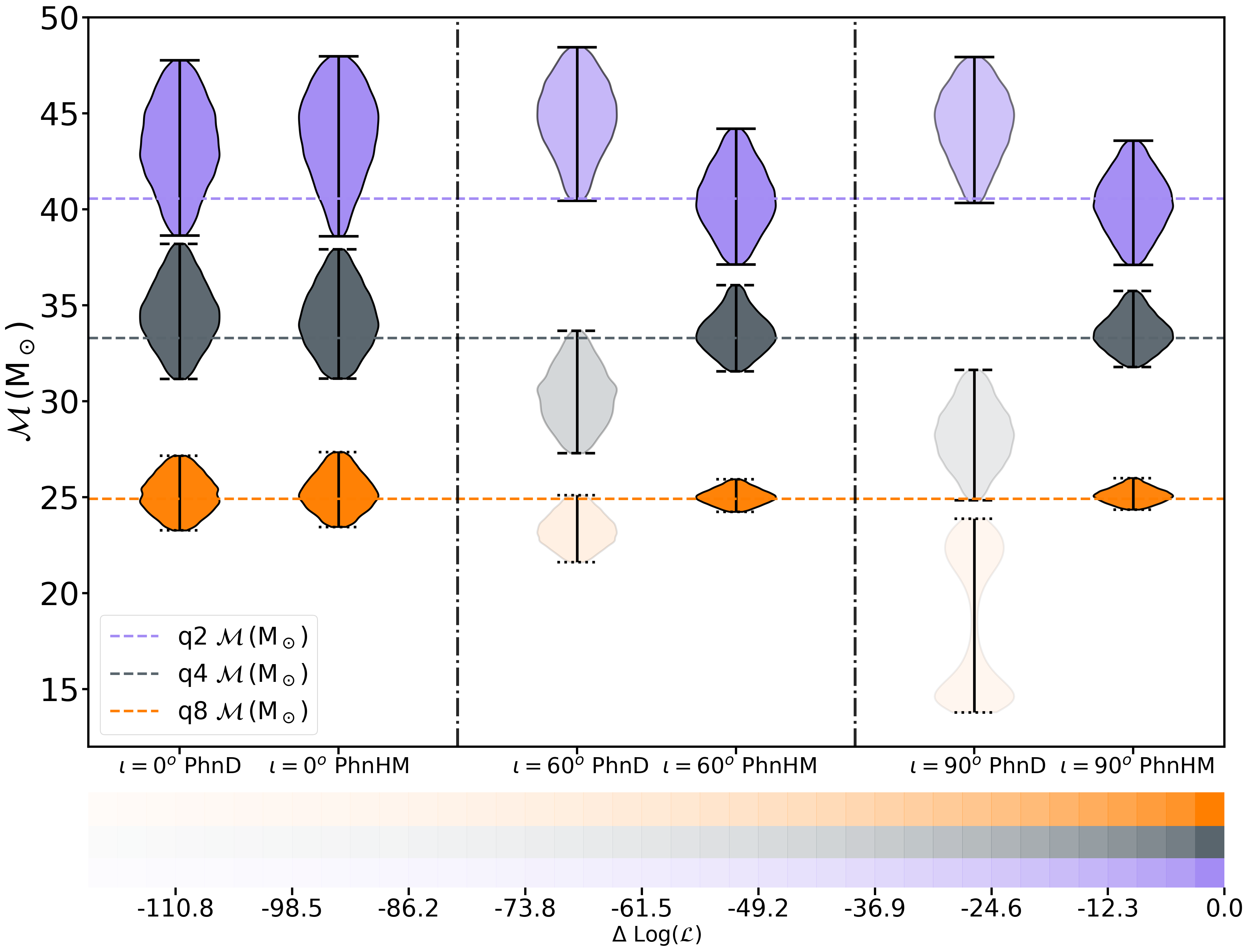
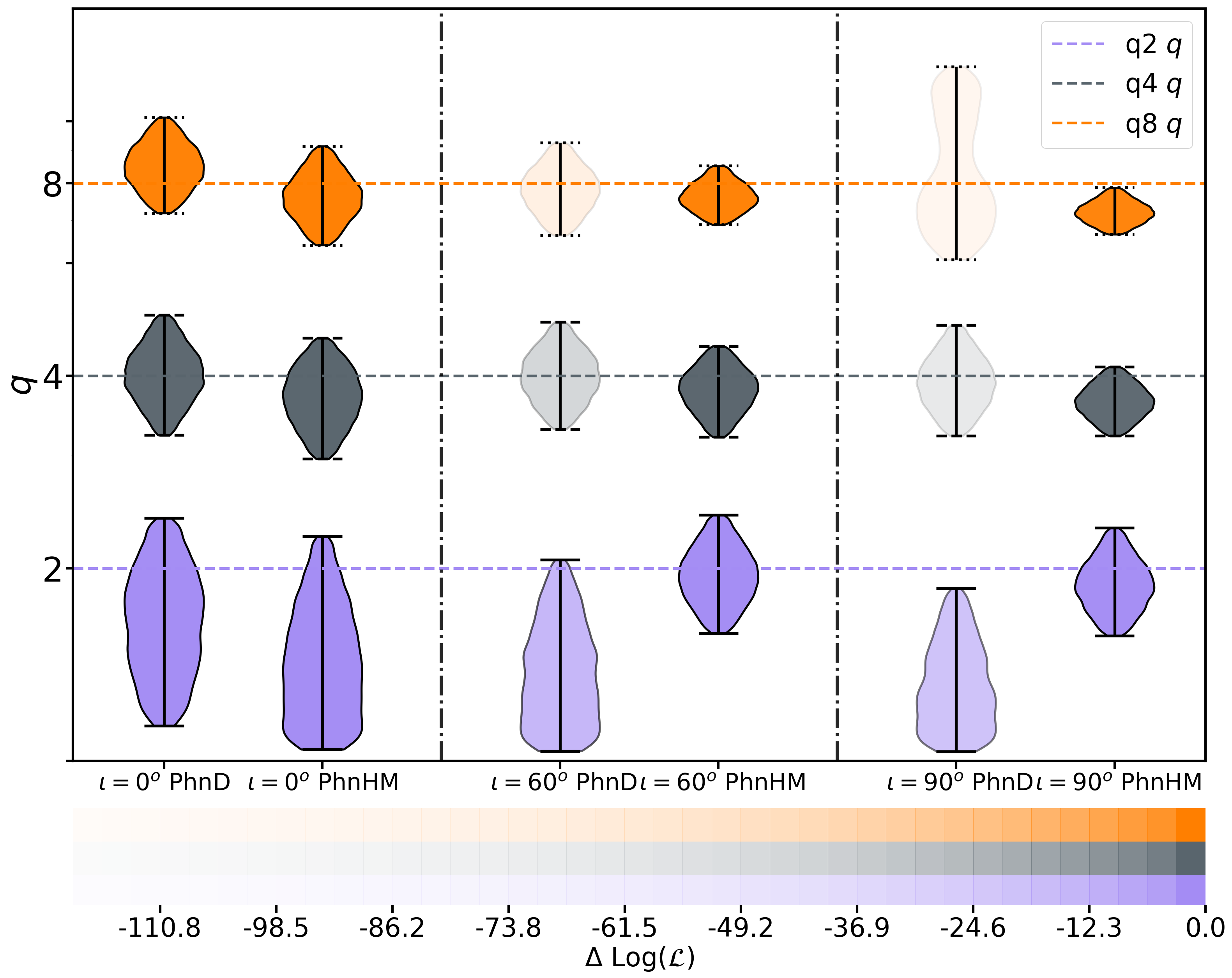
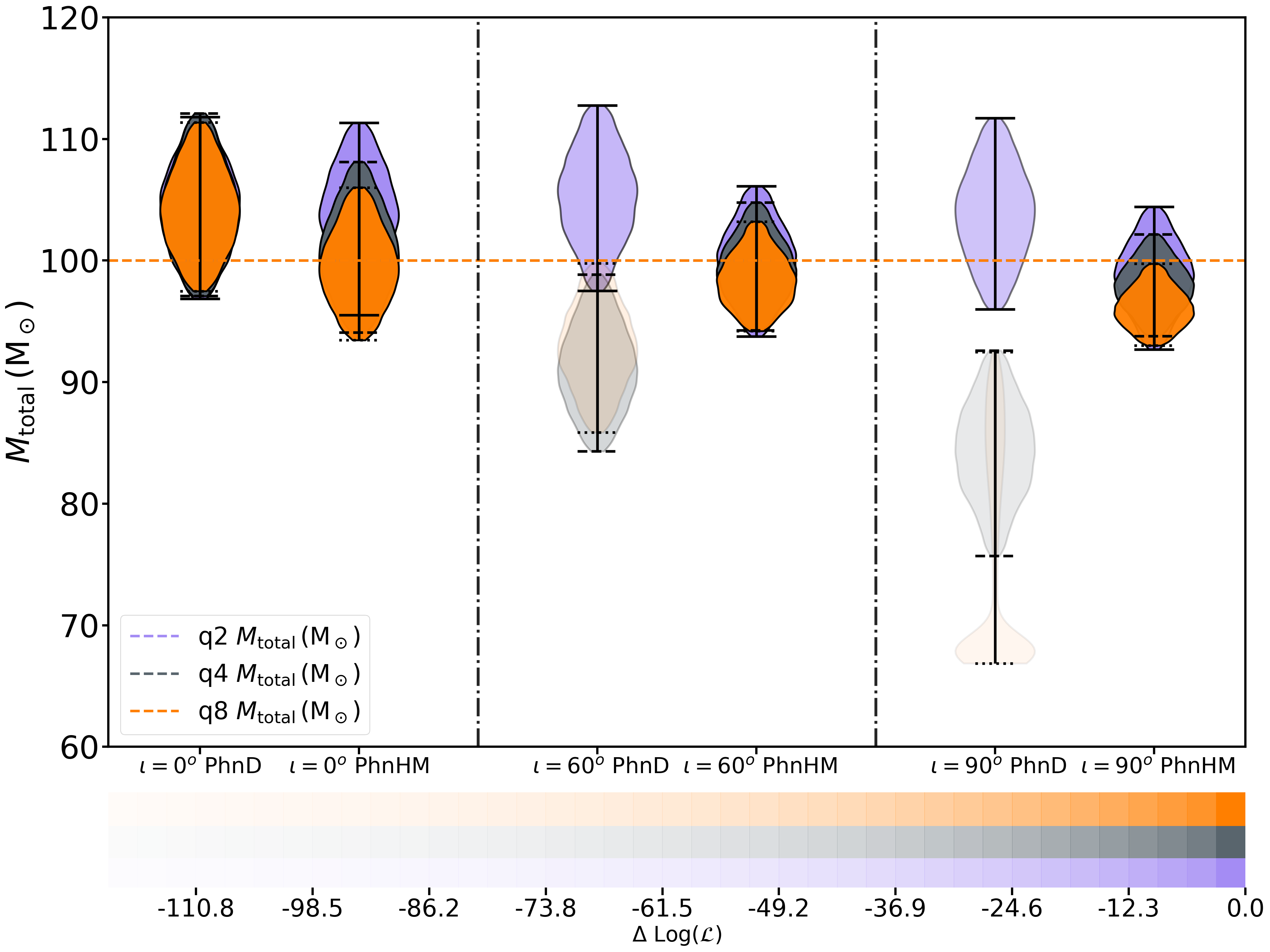
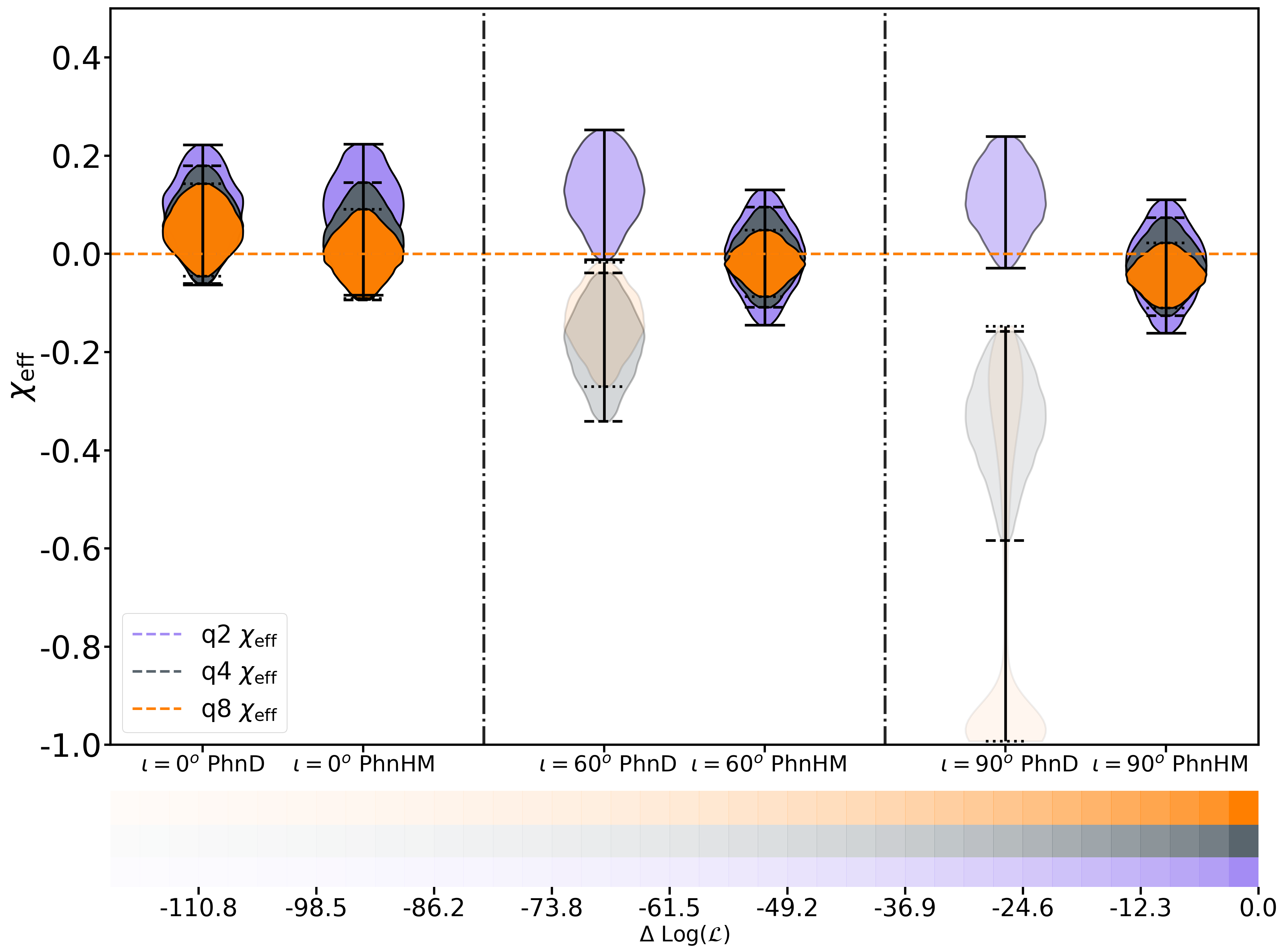
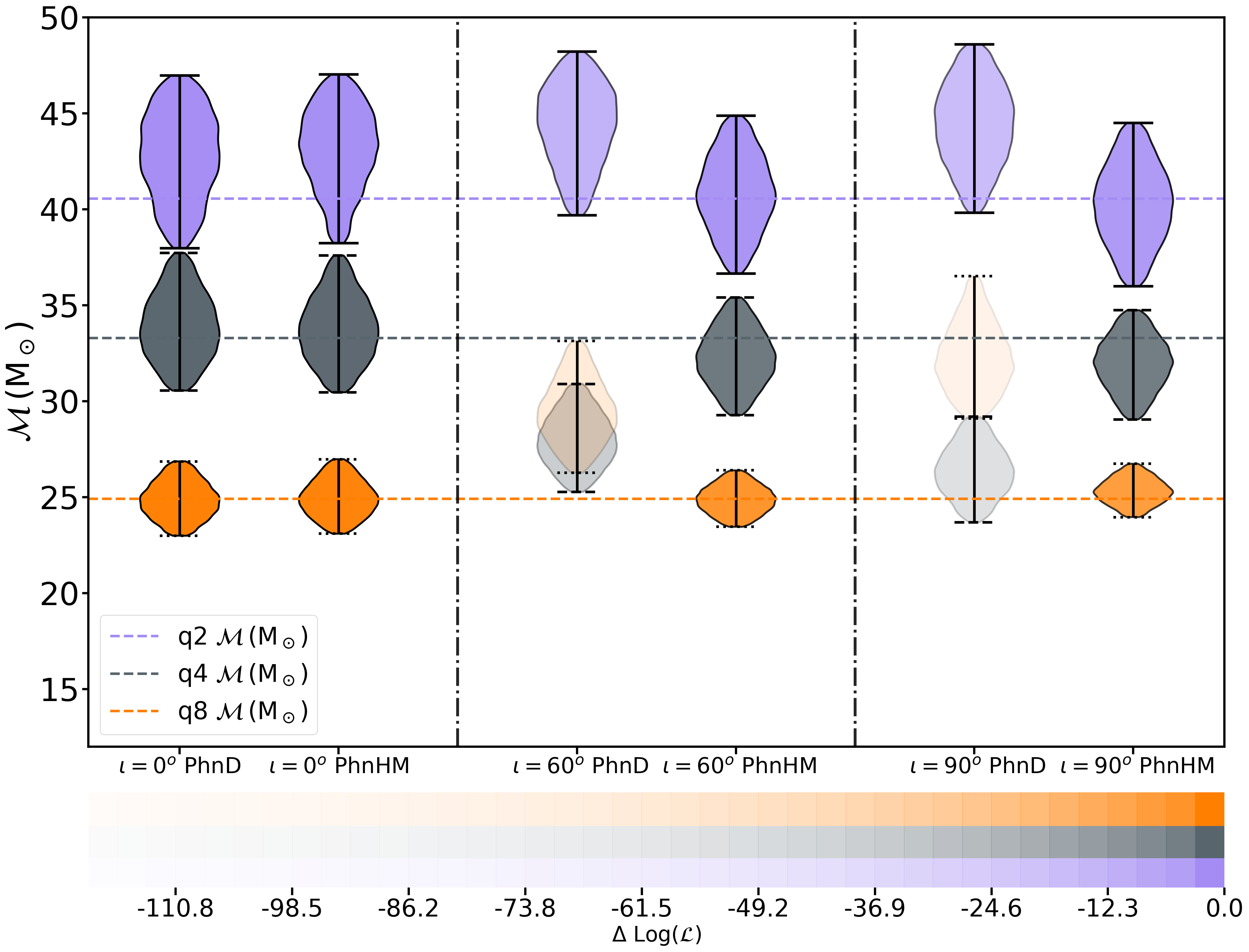
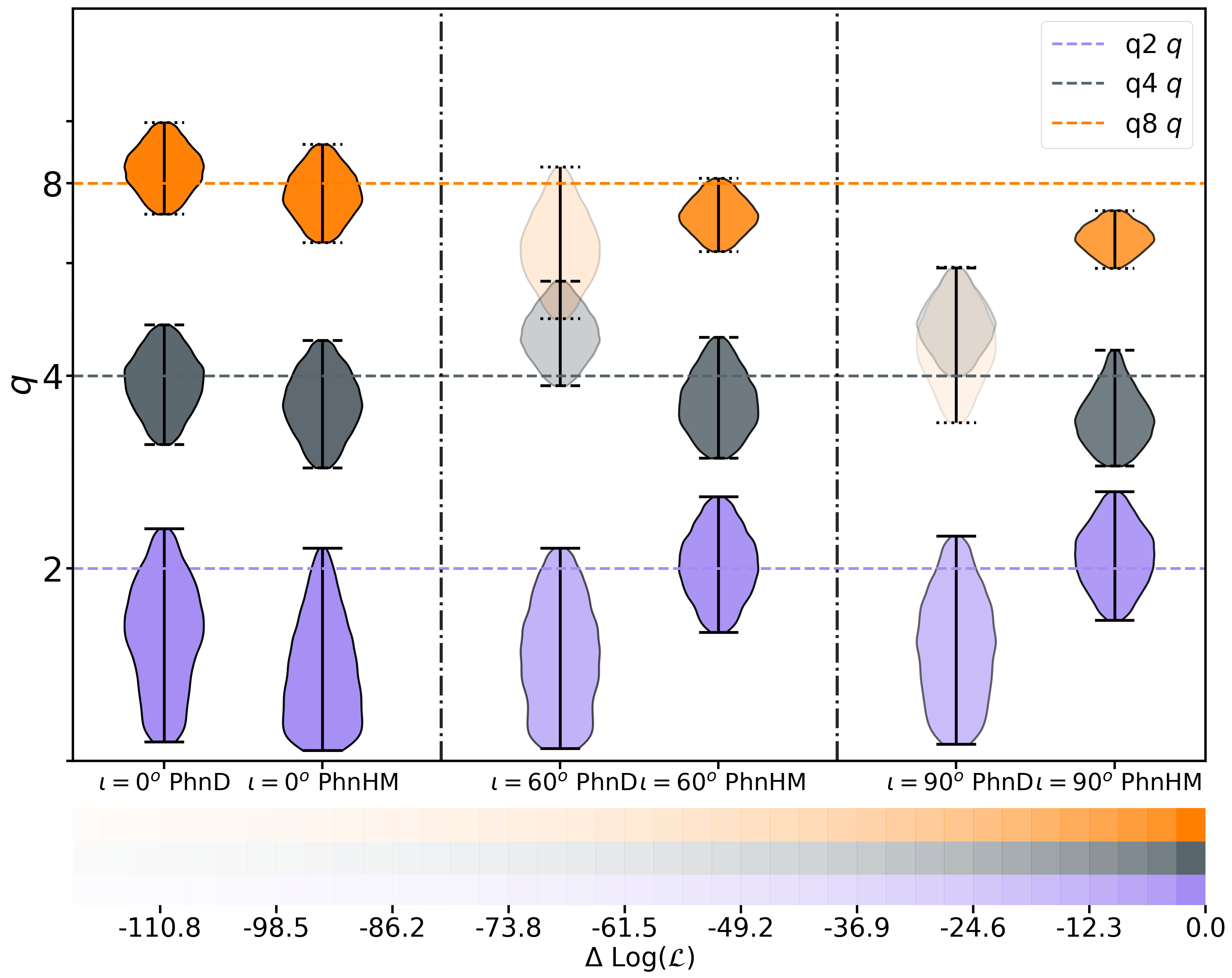
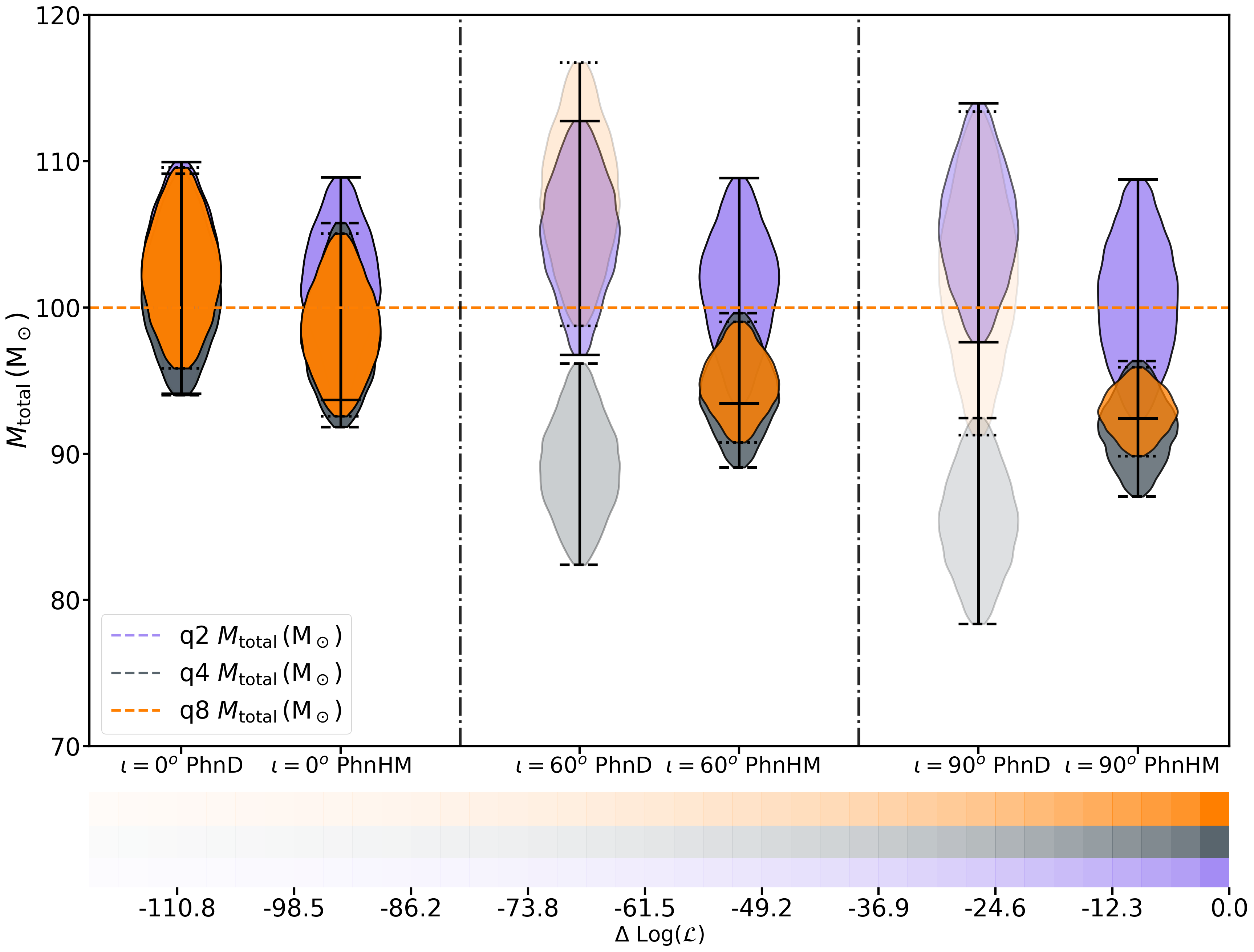
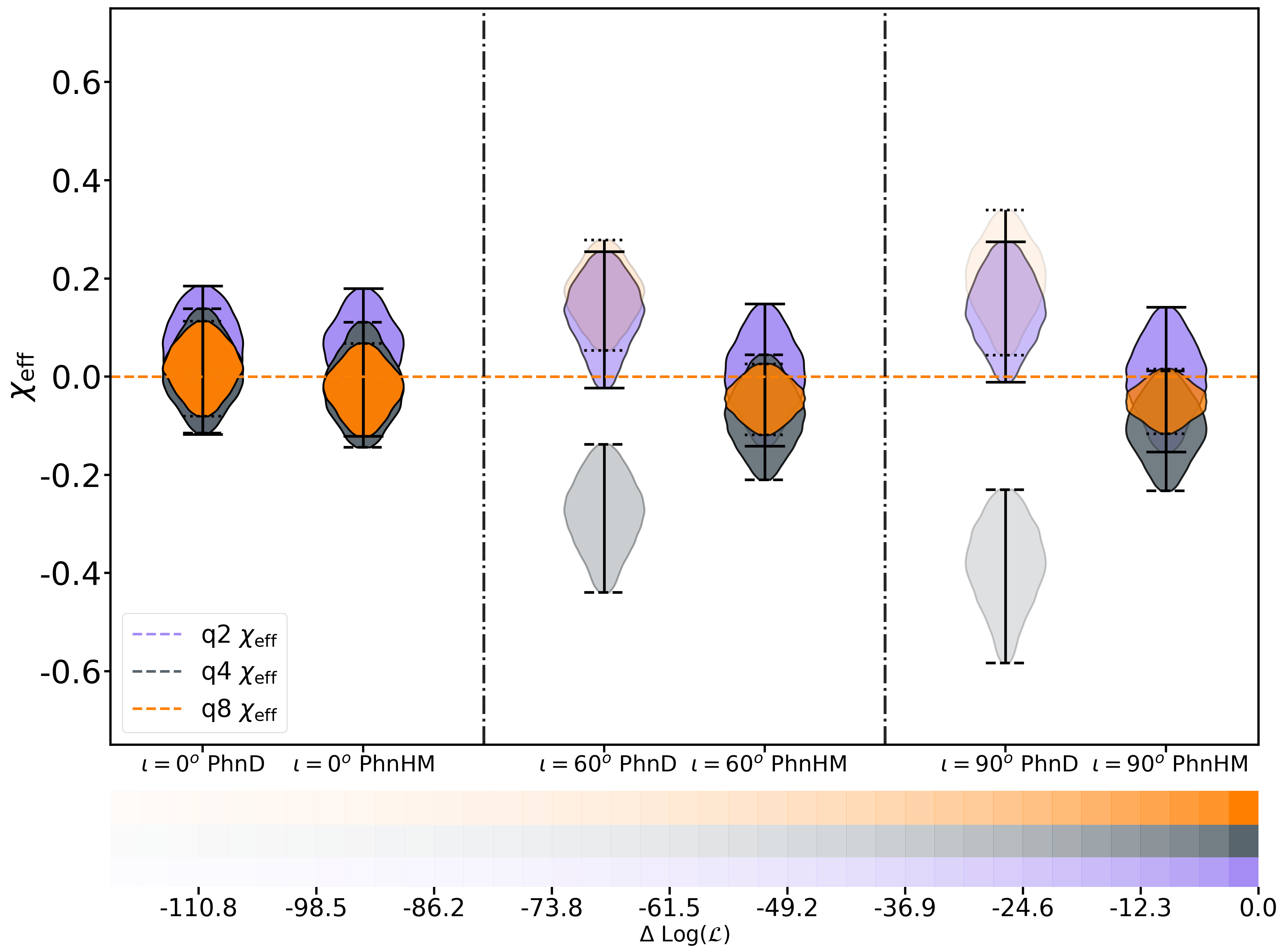
Figure 2: Posteriors of intrinsic parameters $(\mathcal{M}_{c},q,M_{\rm total}(M_{\odot}),\chi_{\rm eff})$ for IMRPhenomHM waveform injected at $q=2$, $q=4$, $q=8$ with $\theta_{JN}$=0, 60^∘, 90^∘. Posteriors for $q=2$ ($q=4$) [$q=8$] are shown in Blue (Grey) [Orange] with the opacity of each determined from the maximum likelihood value of that run. The variation of opacity over the likelihood values is shown at the bottom of each graph. See Sec: III.0.1 for a description of these results, specifically, the bi-modal posteriors recovered by IMRPhenomD at q=8, $\theta_{JN}=$ 90^o.

Figure 3: Posteriors of intrinsic parameters $(\mathcal{M}_{c},q,M_{\rm total},\chi_{\rm eff})$ for Hybrid-NR waveform injected at $q=2$, $q=4$, $q=8$ with $\theta_{JN}=$ 0, 60^∘ and 90^∘. Posteriors for $q=2$ ($q=4$) [$q=8$] are shown in Blue (Grey) [Orange] with the opacity of each determined from the maximum likelihood value of that run. The variation of opacity over the likelihood values is shown at the bottom of each graph.

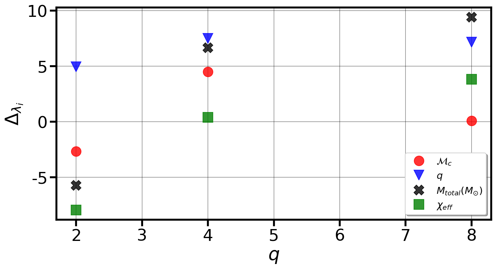
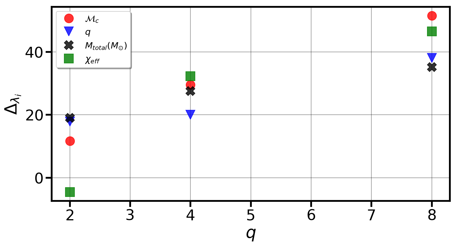
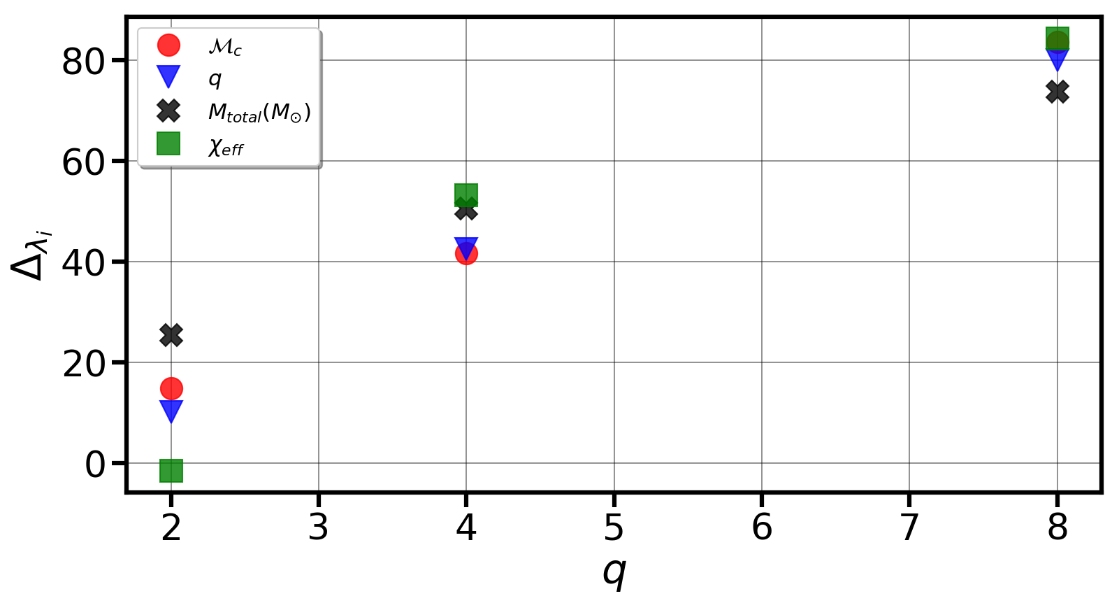
Figure 4: Plot of $\Delta_{\lambda_{i}}$ for all the IMRPhenomHM injections. Results for face-on, 60^∘ and 90^∘ inclination injections are shown in the top, middle and bottom panels respectively. $\Delta_{\lambda_{i}}$ for the parameters $(\mathcal{M}_{c},M_{total}(M_{\odot}),q,\chi_{\rm eff})$ are shown with red-circle, black-cross, blue-lower triangle and green-square respectively.

For a given (mass-ratio, inclination) configuration, the improved constraints on the inclination and distance parameters by using multi-mode templates might lead to better constraints on the intrinsic parameters. To check for that, let us define $d^{model}_{\lambda_{i}}=C^{upper}_{\lambda_{i}}-C^{lower}_{\lambda_{i}}$, where $C^{upper}_{\lambda_{i}}$ and $C^{lower}_{\lambda_{i}}$ are the upper and lower bounds of the 90% CI for a given parameter $\lambda_{i}$. Hence, $d^{model}_{\lambda_{i}}$ would provide a measure of the posterior width. Using this, we define the relative percentage difference between the credible interval widths for a given configuration ($\Delta_{\lambda_{i}}$) as,

$$\Delta_{\lambda_{i}}=100\left(\frac{d^{\texttt{IMRPhenomD}}_{\lambda_{i}}-d^{\texttt{IMRPhenomHM}}_{\lambda_{i}}}{d^{\texttt{IMRPhenomD}}_{\lambda_{i}}}\right).$$ (12)

For a given intrinsic parameter, $\Delta_{\lambda_{i}}$ would quantify the improvements on the parameter constraints from using multi-mode templates.

For the following plots, the posterior over a parameter from each run is clipped within its 90% credible intervals and we plot them as a violin plot. For each parameter, the y-axis shows the value of the recovered posterior and the x-axis gives the injected inclination-recovery waveform combination. For example, if the recovery is for an edge-on injection by IMRPhenomD, it is labelled as $\iota=90^{\circ}\text{PhnD}$. Posteriors for $q=2,4,8$ systems are shown in Blue, Grey and Orange respectively. We will first discuss the results of IMRPhenomHM injections.

III.0.1 IMRPhenomHM Injections

The results of recovered intrinsic parameters for the IMRPhenomHM injections are given in Fig. 3. The percentage improvement in parameter measurements, $\Delta_{\lambda_{i}}$, is shown for $\lambda_{i}\in(\mathcal{M}_{c},M_{\rm total},q,\chi_{\rm eff})$ in Fig. 4.

We consider the face-on systems first, which are the left-hand columns in each of the panels in Fig. 3, and the upper panel in Fig. 4. For all mass ratios, at face-on inclination the posteriors recovered by IMRPhenomHM and IMRPhenomD are consistent with each other, show no bias and are recovered at very similar maximum likelihood. This is expected due to the almost zero contributions ($<10\%$) of higher-order modes to total signal power at face-on inclination and due to the underlying quadrupole model for IMRPhenomHM being IMRPhenomD.

The log Bayes factor between IMRPhenomHM and IMRPhenomD $\log(B^{PhnHM}_{PhnD})$ for all face-on systems is $\leq 4$. At $q=2$, the confidence intervals are almost identical between IMRPhenomHM and IMRPhenomD recovery, although the mass-ratio recovery shows a greater preference for lower $q$. Any improvements in the measurement precision are difficult to detect in the posterior plots, but are clear in Fig. 4. We see that $q$ is always recovered slightly better by IMRPhenomHM  even for the $q=2$ system, with an improvement of $\sim$5%, with the recovery of the other parameters slightly less constrained at $q=2$. Although the effect is small, for face-on signals, the higher-mode content does lead to a slight improvement at higher mass ratios, where we see that the total mass and effective spin are recovered more accurately, and the effective spin measurement is also more precise.

Now consider systems with inclination 60$\degree$. The effects of higher modes are perhaps the most relevant for these cases, because this is where we statistically expect to observe greater number of signals; this is clear from, for example, the IMRPhenomD inclination recoveries in Fig. 5, which predominantly recover the observational prior. In the middle column of each Fig. 3 panel, we see that the IMRPhenomD recovery starts to show a bias away from the true values and the parameters are recovered at comparatively lower likelihood. These effects are stronger with increasing sub-dominant mode contribution to total signal power. At $q=2$, the IMRPhenomD recovery of $\mathcal{M}_{c}$ and $M_{\rm total}$ are slightly biased away from the true value towards overall higher total mass and more equal mass. For a given $q$, the waveform length decreases (increases) at higher (lower) total mass or more negative (positive) $\chi_{\rm eff}$. For the $q=2$ system, the shift to an overall higher total mass is compensated by higher $\chi_{\rm eff}$ recovery. We might expect that the increase in total mass puts more power into the signal, to mimic the extra power that is there from the higher harmonics, but we see the opposite trend for mass ratios $q=4$ and $q=8$. Regardless of the parameter shifts in the quadrupole-only model to find the best agreement with the higher-mode signal, it is clear that best matching IMRPhenomD signals does not agree especially well with the true signal, as indicated by the drop in log-likelihood for signals with increasing mass ratio.

Biases in IMRPhenomD recovery increase with inclination and are most extreme for edge-on cases. Note that there are also biases in the IMRPhenomHM recovery, but these are caused by the prior. The inclination prior has very low support from edge-on inclinations, and hence, the recovered $\theta_{JN}$ posterior tends to have more support from non-edge-on inclinations. This leads to an overestimation of the distance. The amplitude ($\mathcal{A}$) of a BBH source is $\mathcal{A}\propto\mathcal{M}_{c}^{5/6}/d_{L}=M^{5/6}\sqrt{\eta}/d_{L}$. At higher masses, $\mathcal{M}_{c}$ and $M_{\rm total}$ are the better constrained mass parameters. Hence, overestimating $d_{L}$ (with good constraints on $\mathcal{M}_{c}$ and $M_{\rm total}$) would lead to a higher value of $\eta$ or, equivalently, a lower $q$. This effect is what causes the slight bias on the IMRPhenomHM recovered $q$ for edge-on $q=4$ and $q=8$ IMRPhenomHM injections.

Returning to the IMRPhenomD recovery biases, the most extreme case we see is that of the IMRPhenomD recovery of the $q=8$ edge-on IMRPhenomHM injection. The recovered posteriors show a bi-modal distribution. For this injection, IMRPhenomD sees the signal as two completely different systems with parameters $[(M_{\rm total},q,\chi_{\rm eff})\sim(85,7,-0.25),(63,11,-1.)]$, with comparable (but overall very low) likelihood. Including the prior difference, the posterior values around those two areas in the parameter space are very similar, leading to the bimodality. As an additional test, we checked that the bi-modal distribution is not due to sampling error by performing two additional nested-sampling PE runs with 2048 and 4096 live points and another MCMC run with 16 parallel chains and 5000 effective samples, but the bi-modal distribution persists. Two additional PE runs were then done where the sky-position of the signal was randomized while keeping the polarisation fixed and vice versa. The bi-modality seen by IMRPhenomD for the the run in Fig. 3 is lost for these runs, but the corresponding parameters recovered by IMRPhenomD were 1) highly biased and 2) recovered with similar low maximum likelihood ($\Delta Log(\mathcal{L})\sim$ -95). The bi-modality of recovered parameters in Fig. 3 is a consequence of IMRPhenomD seeing the signal as from two different but equally likely systems, which is then lost when the signal morphology changes with changing sky-position and polarisation values. But, for all sky-position and polarisation combinations, parameters recovered by IMRPhenomD for $q=8$ show a consistent bias towards lower total mass and negative $\chi_{\rm eff}$. Also, $\log(B^{PhnHM}_{PhnD})$ for the bi-modal run is $\approx$ 94, which implies that the signal as seen by IMRPhenomD is highly unlikely as compared to IMRPhenomHM. All this suggests that the observed bi-modality is a combined effect of the priors over the physical parameters and the inaccuracy of IMRPhenomD towards recreating the true multi-mode signal.

$\mathcal{M}_{c}$ posteriors recovered by IMRPhenomHM are accurate for all the cases. At face-on $q=2$, recovered $q$ has large support from near-equal mass systems, but this behaviour is lost at higher inclinations. At edge-on $q=4$ and $q=8$, mass-ratio and $M_{\rm total}$ are slightly biased towards lower values, with accurate recovery of the mass-spin parameters for all other cases.

Where quadrupole models tend to recover a biased $\chi_{\rm eff}$ at higher inclinations, IMRPhenomHM recovery does not. For the $q=2$ injections with $\theta_{JN}=$ 60^∘ and 90^∘, the recovered $\chi_{\rm eff}$ posteriors have almost the same width for IMRPhenomD and IMRPhenomHM templates ($\Delta_{\chi_{\rm eff}}\sim 0$). Although the spread of these posteriors is similar, $\chi_{\rm eff}$ recovery with IMRPhenomHM is accurate, whereas IMRPhenomD recovery is biased.

We now consider the relative improvement in parameter precision (i.e., the widths of the posteriors, irrespective of any bias from the true injected values), as shown in Fig. 4.

At inclinations of 60^∘ and 90^∘, the mass parameters recovered by IMRPhenomHM are always better constrained than corresponding IMRPhenomD recoveries (see middle and bottom panels of Fig. 4), i.e., $\Delta_{\lambda_{i}}>0$. For a given inclination-parameter combination, $\Delta_{\lambda_{i}}$ increases with increasing $q$. For e.g., for $\theta_{JN}=$ 60^∘, $\Delta_{\mathcal{M}_{c}}\sim 20\%,30\%,50\%$ for $q=2$, 4 and 8 respectively. The comparatively high $\Delta_{\lambda_{i}}$ values for the edge-on $q=8$ configuration is due to the bi-modality of the IMRPhenomD recovered posteriors. At $q=4$ and $q=8$, $\Delta_{\chi_{\rm eff}}\geq 0$ for all inclinations, and IMRPhenomD recovers biased $\chi_{\rm eff}$ posteriors for non-face-on inclinations whereas IMRPhenomHM recovery is accurate for all configurations. Overall, we observe better constraints on the mass parameters for inclined system across the mass-ratio space.

The results in Fig. 4 illustrate that in addition to more accurate parameter recovery when using a multi-mode model, we also find improved precision in the parameter measurements. We see that other than for face-on configurations, the recovered mass and spin parameters are better constrained ($\Delta_{\lambda_{i}}>0$), with the constraints improving with increasing mass-ratio and/or inclination.

III.0.2 Hybrid-NR Injections

We now consider injections of the same physical systems, but using hybrid-NR waveforms instead of IMRPhenomHM. The purpose of this is to assess systematic errors in the IMRPhenomHM model. If the hybrid-NR waveforms and the corresponding IMRPhenomHM waveforms were almost identical, then the results from hybrid-NR injections would be nearly identical to those in the previous section. This would require not only that the IMRPhenomHM model accurately capture all of the features of the NR waveforms, but that the numerical errors in the higher-mode content of the NR waveforms be insignificant, along with the differences between the hybrids’ EOB inspiral and the IMRPhenomHM inspiral. We do not expect any of these requirements to hold, and so with hybrid-NR injections we can determine which of the previous results is robust against uncertainties in the IMRPhenomHM model, and for which parameters and regions of the parameter space systematic errors may contaminate measurements.

The results of recovered intrinsic parameters for Hybrid NR waveform injections are given in Fig. 3. For these injections, we will not plot the $\Delta\lambda_{i}$s, but will discuss them when relevant. For $q=2$, $q=4$ and $q=8$, at face-on inclinations, posteriors recovered by IMRPhenomHM and IMRPhenomD follow the same behaviour that we saw for IMRPhenomHM injections. Parameters recovered by both models are accurate, but the posteriors recovered by IMRPhenomHM show slightly improved constraints on the mass and spin parameters ($\Delta_{\lambda_{i}}\geq 0$). Given the weak higher-mode content in face-on injections, it is not surprising that the results do not depend strongly on whether IMRPhenomHM or hybrid-NR waveforms were injected.

The same is true for $q=2$ injections at all inclinations. In some cases the posteriors are wider for the hybrid-NR injections, the most notable example being the IMRPhenomHM recovery of $M_{\rm total}$ at $\theta_{JN}=$ 60$\degree$. However, it is not too surprising that recovery is more accurate and precise when the injection was an instance of the waveform model used for recovery, as with the IMRPhenomHM injections. The lack of any notable impact of systematic errors at $q=2$ means that the bias in the quadrupole-only recovery of $\chi_{\rm eff}$ for the 60$\degree$ injection is a robust result.

For $q=4$ and $q=8$ injections, we do see some clear differences between the results from IMRPhenomHM and hybrid-NR injections. To ease the interpretation of a large number of results, we first focus on the the recovery using IMRPhenomHM, which is most relevant to future GW observations. Here we see that for most parameters the recovery again does not change significantly between the two classes of injections. There are two exceptions. One is the recovery of the mass ratio for $q=8$ edge-on systems, where we see that the prior effect, which leads to an underestimation of $q$, becomes yet more pronounced with the hybrid-NR injection, and the true value is outside the 90% C.I. The other is the measurement of the total mass. The posteriors are broader in the $q=2$ case for both 60^∘ and edge-on configurations, and for $q=4$ and $q=8$ the mass is clearly biased. However, we also note that these are cases where the quadrupole-only IMRPhenomD shows extremely large biases, and the IMRPhenomHM recovery shows a clear improvement.

As with the biases on mass parameters, biases on IMRPhenomD recovered $\chi_{\rm eff}$ for the hybrid-NR injections follow the same behaviour as for IMRPhenomHM injections for $q=$ 2 and 4, but the bias for $q=8$ is in the opposite direction. However, IMRPhenomHM is able to measure the true value of $\chi_{\rm eff}$ within its 90% CIs for all the configurations.

If we now look at the quadrupole-only recovery, we see that there are many differences between the IMRPhenomHM and hybrid-NR injections. Some of these are counter-intuitive: for example, for the $q=8$ - 60^∘ injections, the bias in the chirp mass recovery is in opposite directions for the two classes of injections. However, we note that in all of these examples, the log-likelihood for the IMRPhenomD recovery is low, and so it is possible for the parameters of best agreement between IMRPhenomD and the injected waveform to show greater variation; and note also that these will also be sensitive to all of the intrinsic and extrinsic parameters.

Overall we conclude that only in the most extreme cases ($q=8$ and edge-on) do we see a risk of biases when using IMRPhenomHM for parameter recovery, and in all cases it shows an improvement, and often a dramatic improvement, over a quadrupole-only model.

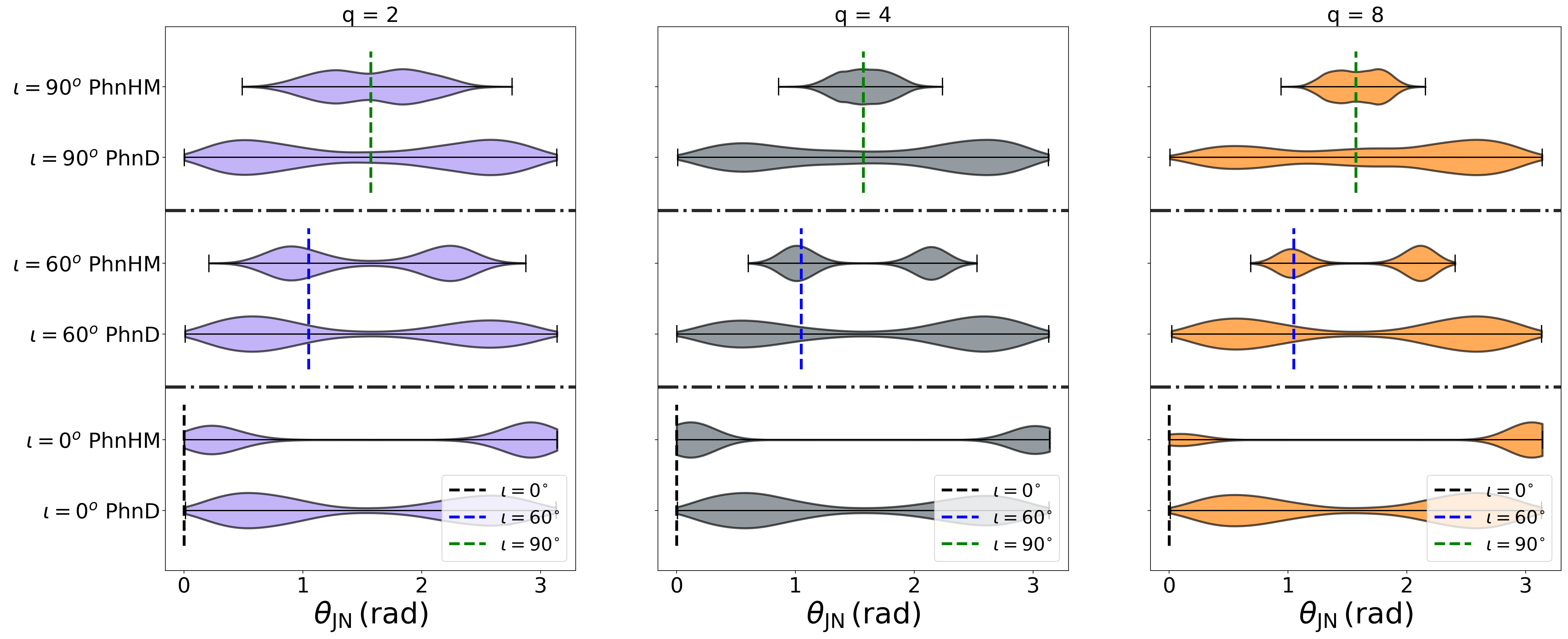
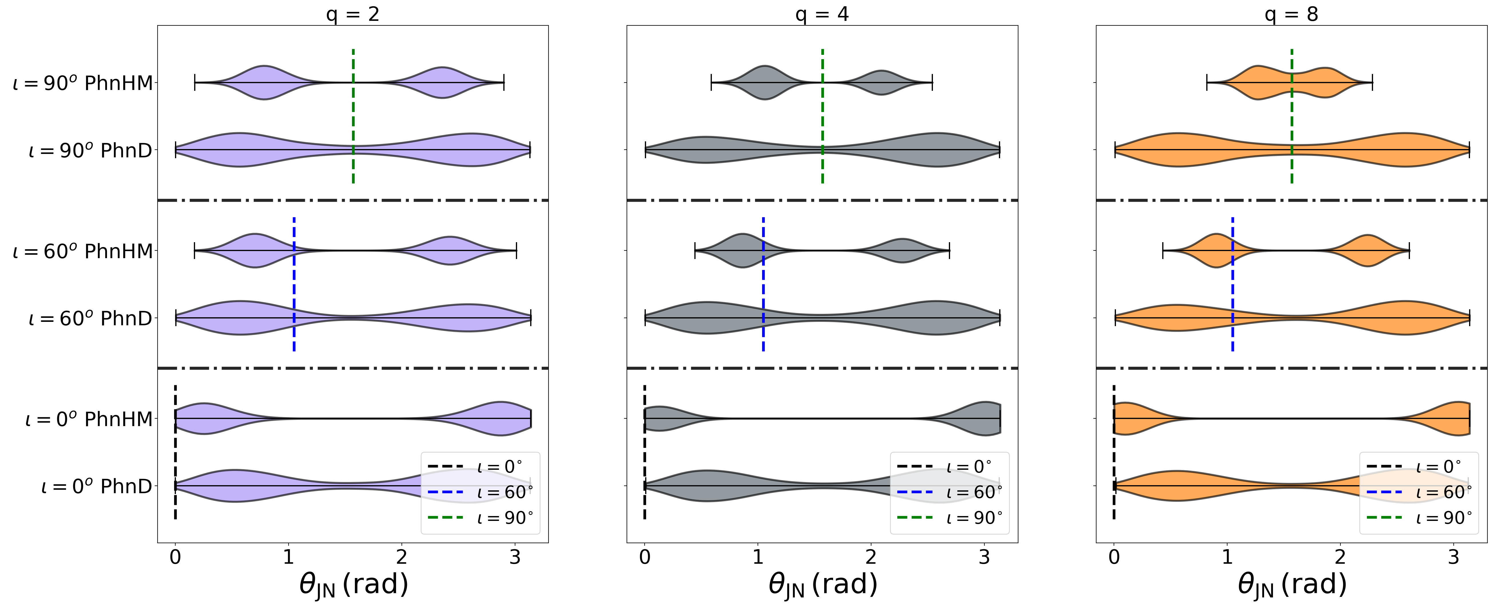
Figure 5: Recovery of $\theta_{JN}$ for IMRPhenomHM injection (top row) and hybrid NR injections (bottom row) for inclinations 0, $60^{\circ}$ & $90^{\circ}$ and with IMRPhenomHM and IMRPhenomD as recovery waveform models. Inclination recovery for $q=2,4,8$ configurations are shown in the left, centre and right columns respectively, with the recovery for each inclination separated by horizontal dashed-black lines. The true value of the injections are given in dashed Black, Blue and Red lines for 0, $60^{\circ}$ & $90^{\circ}$.

IV Recovery of extrinsic parameters

We saw in Ref. London et al. (2018) that one of the most significant impacts of using a higher-multipole model for parameter measurement is in the recovery of the binary’s inclination ($\theta_{JN}$) and distance ($d_{L}$). In a quadrupole-only model, the only effect of changing the inclination is to change the overall amplitude, which is degenerate with a change in distance. The strength of the $(2,2)$ mode varies by a factor of two between face-on and edge-on systems (for the plus polarisation), leading to an uncertainty of roughly a factor of two in the distance measurement. The inclination measurement is then dominated by the prior, which is a combination of the inclination dependence of the detector sensitivity (the sensitivity is twice as sensitive to face-on systems) and the inclination probability distribution, which is uniform in $\cos(\theta_{JN})$. The result is a distribution that peaks at $\sim$30$\degree$ and $\sim$150$\degree$, and this is reflected in the IMRPhenomD inclination recovery plots below. In general, as was seen in Ref. Graff et al. (2015); Littenberg et al. (2013); O’Shaughnessy et al. (2014a, b), the use of higher-order mode templates break the degeneracy present between $\theta_{JN}$, $\psi$ and $\phi$ that allows for better measurements of inclination value and hence better distance precision. We see that IMRPhenomHM is able to capture inclination information better than IMRPhenomD and leads to improved constraints on the distance.

In the following sections we quantify these effects for both IMRPhenomHM and hybrid-NR injections; the former quantify the impact of higher multipoles, while the latter allow us to investigate systematic biases due to approximations in IMRPhenomHM.

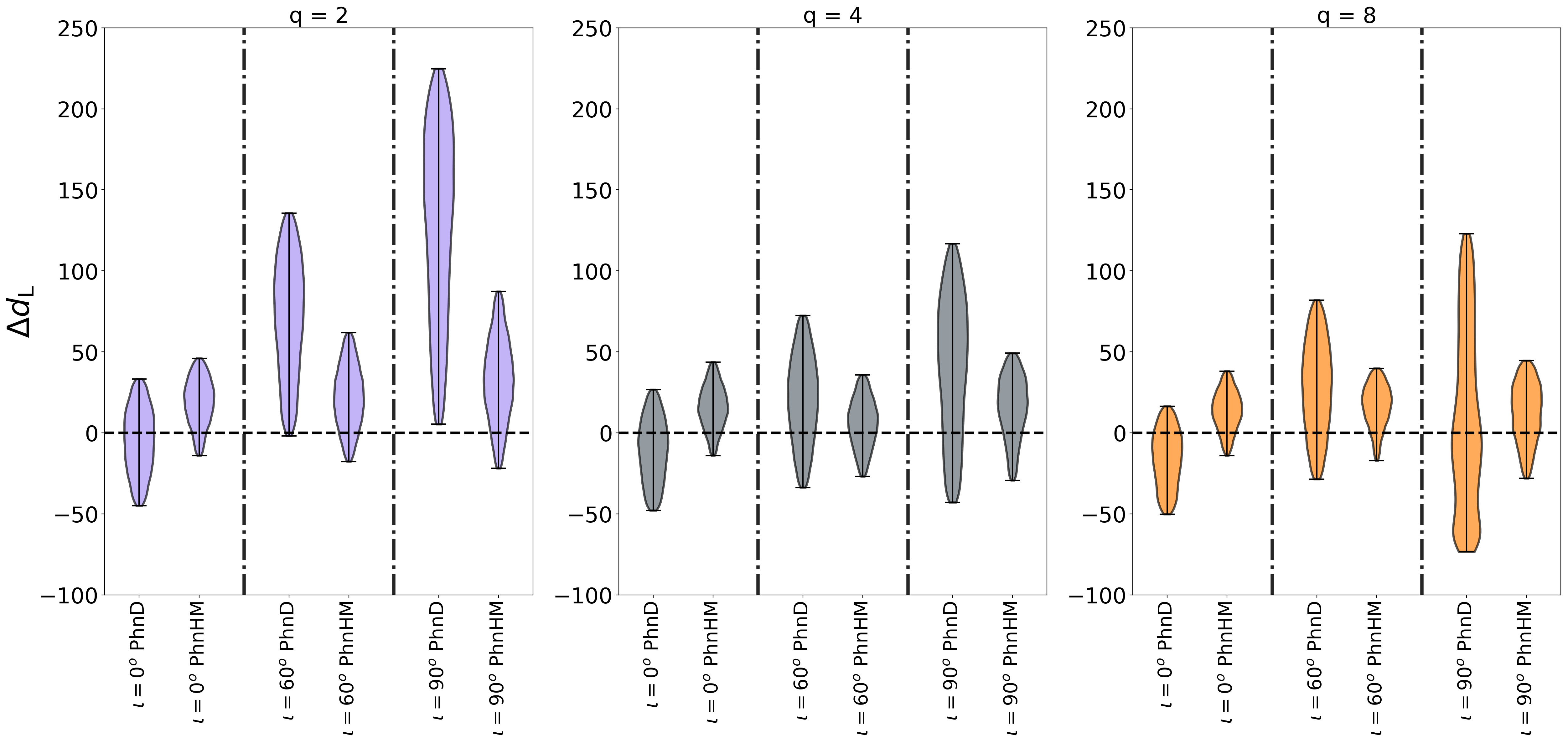
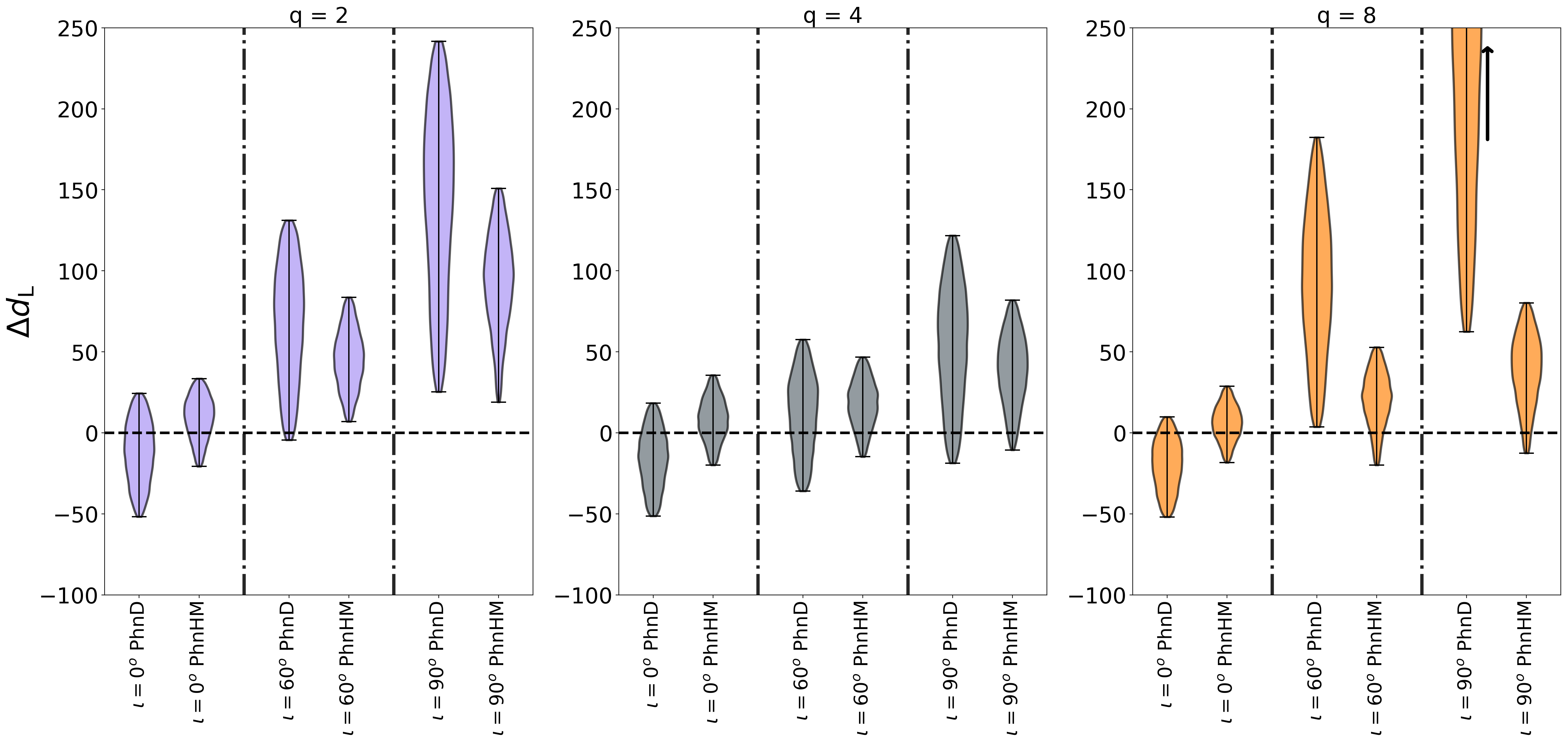
Figure 6: Recovered percent distance error $\Delta d_{L}$ (see Eq:13) recovery for IMRPhenomHM injection (top row) and Hybrid NR injections (bottom row) for inclinations 0, 60^∘ and 90^∘ with IMRPhenomHM and IMRPhenomD as recovery waveform models. Distance recovery for $q=2,4,8$ configurations are shown in the left, center and right columns respectively. The $\Delta d_{L}$ = 0 line is shown in horizontal dashed-black line, with the vertical dashed lines separating recovery for different inclinations. The injected distance value for IMRPhenomHM [NR] injection for $q=(2,4,8)$ 0$\degree$ is (895, 624, 388) [880, 639, 398] Mpc, 60$\degree$ is (537, 404, 258) [523, 376, 249] Mpc and for 90$\degree$ is (387, 307, 199) [367, 253, 183] Mpc. For the $q=8$, 90$\degree$ hybrid-NR recovery by IMRPhenomD, $\Delta d_{L}$ extends up to 400%.

IV.0.1 $\theta_{JN}$ recovery

Fig. 5 shows the results for inclination recovery for both the IMRPhenomHM and hybrid-NR injections. For both IMRPhenomHM and hybrid NR injections, at all mass-ratio and inclination configurations, $\theta_{JN}$ recovery by IMRPhenomD shows a similar bimodal behaviour and mostly follows the prior, as discussed above. Inclination recovery is unaffected by mass-ratio or inclination value for the quadrupole only model and thus it is not possible to differentiate between a non-inclined and inclined system.

For IMRPhenomHM recovery, the bi-modality for the inclination posterior persists, but the posteriors are better constrained. At face-on configurations for IMRPhenomHM and hybrid NR injections, IMRPhenomHM sees the system as strongly face-on or face-off. For 60^∘ IMRPhenomHM injections, the recovered inclination is peaked near the true value and the constraint on the inclination improves with increasing mass-ratio. The edge-on IMRPhenomHM injection posteriors show a similar behaviour. For Hybrid NR injections, inclination recovery for 60^∘ is peaked just off the true value and for edge-on $q=(2,4)$ systems, the recovery is strongly biased. This is not surprising: the systematic errors in the IMRPhenomHM model enter almost entirely into the higher multipoles, and so the largest systematic errors will be observed for edge-on systems, where the higher multipoles contribute most to the signal. We find, however, that it is only for the edge-on cases that this bias appears. Since edge-on systems are still roughly half as strong as equivalent face-on systems, they are eight times less likely to be observed.

IV.0.2 Distance recovery

Recall that injections were made such that the signal’s SNR was 25 in all cases. Since the signal strength decreases as mass-ratio increases, and also as the inclination varies from face-on to edge-on, the edge-on $q=8$ system is injected at a much smaller distance (199 Mpc) than the face-on $q=2$ system (895 Mpc). Although there is some variation in the injection distance between the IMRPhenomHM and hybrid-NR injections, due to the differences in their higher-multipole content; these are small and are always less than 10%. All of the injection distances are given in the caption to Fig. 6.

Fig. 6 shows the results for distance recovery. We plot the relative percent distance error, which we define as,

$$\leavevmode\nobreak\ \Delta d_{L}=100\left(\frac{d_{L}^{\rm posterior}-d_{L}^{\rm injected}}{d_{L}^{\rm injected}}\right)$$ (13)

For IMRPhenomHM injections, the true distance value lies within the 90% confidence intervals for most of IMRPhenomD and all of IMRPhenomHM recovered posteriors. At larger inclinations, the quadrupole model tends to overestimate the distance to the binary. For $q=2$ Hybrid NR injections, at inclinations 60$\degree$ and 90$\degree$, 90% CIs for $d_{L}$ recovered by IMRPhenomHM  do not include the true value. For all other situations though, 90% CIs for $d_{L}$ recovered by IMRPhenomHM contain the true injected value.

For quadrupole-only templates, as the recovered inclination is the same for all injected inclinations, the recovered distance for non-zero inclinations tend towards overall larger values leading to larger $\Delta d_{L}$. For IMRPhenomHM injection - IMRPhenomHM recovery, where injected $\theta_{JN}$ lies within the 90% CIs of recovered $\theta_{JN}$, the real distance is recovered at all times. For the $q=2$ and $q=4$ hybrid-NR injection - IMRPhenomHM template, recovered $\theta_{JN}$ at 60^∘ (90^∘) is slightly (completely) off the true value which causes the recovered distance to be overestimated from the true value. This is likely due to the different mode content in the signal and template and the waveform inaccuracies in IMRPhenomHM. But, these results do indicate that use of multi-mode template waveform will lead to better distance measurements.

The improved constraints on inclination for IMRPhenomHM  recovery translates to improved constraints on the measured distance of the system as compared to IMRPhenomD recovery. We see this behaviour for all the configurations. At face-on configurations, IMRPhenomHM constrains the distance about $\sim$ 20% - 25% better as compared to IMRPhenomD. For higher inclinations, the constraint improves by about $\sim$ 30% - 60%.

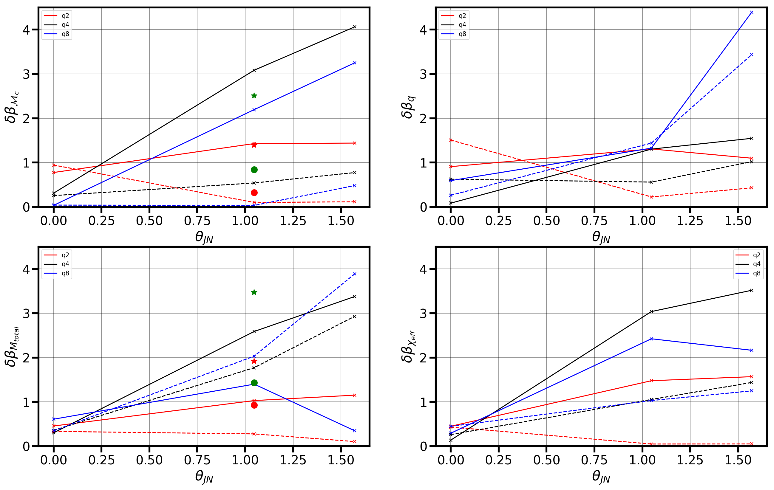
Figure 7: We plot the quantity $\delta\beta_{\lambda_{i}}$ for the parameters $(\mathcal{M}_{c},M_{total},q,\chi_{\rm eff})$ for hybrid-NR injection results with the solid (dashed) lines indicating the bias value for IMRPhenomD (IMRPhenomHM) recovery. $\delta\beta_{\lambda_{i}}$ for $q=2,48$ are shown in Red, Black and Blue respectively. The systematic bias for the $q=2,6$, $M/M_{\odot}=51,56$ and SNR = 48 configurations from Ref. Littenberg et al. (2013) are shown in red (green) with the quadrupole (multi-mode) recovered bias shown with a star (circle).

V Conclusions

This is the first study that quantifies the accuracy of inferred source parameters using a multi-mode aligned-spin model waveform. To do that, we consider two families of non-spinning multi-mode signal waveforms (IMRPhenomHM and hybrid-NR) over a range of mass-ratios ($q=2,4,8)$ and inclinations (face-on, 60$\degree$, and edge-on), with fixed total mass, and compare the parameters recovered by multi-mode and quadrupole-only templates. In all cases we consider a signal-to-noise ratio (SNR) of 25. We fix the total mass of injected signals at 100$M_{\odot}$, for three reasons; i) the relative measurable signal power in the higher modes increases with mass, and so the choice of a high mass allows us to provide an estimate of the largest impact of higher modes in likely LIGO-Virgo observations, for which total binary masses above 100$M_{\odot}$ will be rare. ii) IMRPhenomHM is an approximate waveform model of the sub-dominant modes that is not tuned to NR waveforms, and the most uncertain part of the IMRPhenomHM modelling is in the merger and ringdown phases. Hence, the choice of a high total mass also allows us to also make a conservative estimate of the systematic errors due to waveform inaccuracies. iii) IMRPhenomHM is a more computationally expensive model than its quadrupole-only counterpart, and signals with total mass 100$M_{\odot}$ allow us to quickly perform a large PE study. Although, as previous studies have shown Calderón Bustillo et al. (2016); Varma and Ajith (2017); Varma et al. (2014), systematic errors due to neglecting higher-order modes in template waveforms increase at higher masses. Optimized versions of the model will make it easier to perform a much more extensive study over a wider range of parameters, including much lower masses.

Here is a summary of our main results.

Our key results on measurements of intrinsic parameters are in Figs. 3 and 3. For face-on systems there is no appreciable bias in the quadrupole-only recovery at any mass ratio. There are biases in the total mass of up to 10% at 60$\degree$ inclination, and 20% or 30% for edge-on configurations. For the edge-on $q=8$ configuration (IMRPhenomHM injection), the signal matches the quadrupole-only model so poorly that the recovery is bimodal. Mass ratio is strongly biased toward equal-mass recovery for small mass ratios, but shows less bias at higher mass ratios. (This point is relevant to the observation GW170729 Chatziioannou et al. (2019), where the templates with higher-order modes were able to resolve $q$ between 1.25 and 3.3 at 90% confidence, i.e., providing strong evidence that the mass-ratio was bounded away from equal mass, while quadrupole-only models gave a 90% C.I. from $q=1$ up to $q=2.5$.) The effective spin $\chi_{\rm eff}$ shows a bias of up to 0.2 for 60$\degree$ inclination and cannot be measured at all in some edge-on cases. Our results suggest that bi-modal parameters or, in less extreme cases, double-peaked posteriors, might occur (for some cases) when measuring high-mass-ratio systems with a quadrupole-only model which could be resolved with multi-mode models. The overall lower likelihood of recovered parameters by the quadrupole-only model (compared to multi-mode model) at high-mass ratio - high-inclination combination suggest that the model cannot be trusted for accuracy in that region.

For IMRPhenomHM injections, recovery with a higher-mode model not only removes these biases (as we would expect, since the injection and recovery use the same model), but also increases the precision of the measurement. Fig. 4 shows the percentage improvement in the size of the 90% credible intervals over using a quadrupole-only model. The improvement is up to 50% for 60$\degree$ inclination and up to 80% for edge-on configurations; the improvement is roughly linear with mass ratio . Improvement in parameter recovery was also considered in Ref. Graff et al. (2015), but using a higher-mode model that did not include spin. We find that the addition of the spin dimension can significantly increase the widths of the confidence intervals. For example, recovering a $q=4$, $M=100\,M_{\odot}$, 60$\degree$-inclination SNR=18 signal with a nonspinnng model leads to an uncertainty in the chirp mass of $\Delta\mathcal{M}_{obs}/\mathcal{M}_{obs}=0.056$ Graff et al. (2015). If we naively rescale to an SNR of 25, the uncertainty would decrease to $\sim 0.04$. By contrast, the uncertainty when using a spinning higher-mode model is 0.168, i.e., four times larger.

NR-hybrid injections show broadly consistent results, indicating that the systematic errors in the IMRPhenomHM model are in general small. The IMRPhenomHM recovery gives comparable results between the IMRPhenomHM and NR-hybrid injections, except for biases of up to 5% in the total mass for $q=4$ and $q=8$ non-face-on cases; this is less than the bias incurred by using a quadrupole-only model. Results show larger differences in the IMRPhenomD recovery between the two injection sets, but these are cases where the log-likelihood is poorer, and so we ascribe these less significance. Our conclusion is that the IMRPhenomHM model leads to improved parameter measurements over a quadrupole-only model in all cases; and except for high-mass high-mass-ratio high-inclination signals with an SNR of 25 or higher, systematic errors will not affect results.

This is quantified further in Fig. 7. Here we follow Ref. Littenberg et al. (2013), and plot the ratio of the systematic error to the statistical error, $\delta\beta_{\lambda^{i}}$, for the parameter $\lambda^{i}$. By “systematic error” we mean the difference between the true injected parameter and the mean of the marginalised 1D recovered posterior (in Ref. Littenberg et al. (2013), the authors use the difference between the maximum a posteriori value and injected value), and by “statistical error” we mean the standard deviation of the posterior. Since the standard deviation corresponds to the 68% C.I., $\delta\beta_{\lambda^{i}}$ is a more conservative estimate than if we had used the 90% C.I. As such, if the ratio is below $\sim 1.645$, then the systematic error is within the 90% C.I. and the measurement is not considered to be biased. Fig. 7 shows this error ratio for the chirp mass, total mass, mass ratio, and effective spin. Also shown are the results from Ref. Littenberg et al. (2013), although care should be taken in comparing the results, since that study considered lower masses, higher SNRs and different mode content for the injections.

Inclination recovery is always improved when recovering with a higher-mode model. With quadrupole-only recovery, the distance-inclination degeneracy means that largely the same posterior is recovered, regardless of inclination (see Fig. 5), while the higher-mode model is able to constrain the inclination. The trend in the IMRPhenomD distance recovery is consistent with expectations: for a signal with a high non-zero inclination, a quadrupole only template model gets more support from non-edge on inclinations, suggesting that the (comparatively) weak signal is from further away and therefore $d_{L}$ would be overestimated. A multi-mode template model can better constrain the degeneracy between the inclination, phase and polarisation values, leading to improved constraints on the inclination, which then translates to a better constrained measurement of distance. Distance recovery is greatly improved with the higher-mode model. At face-on configurations, IMRPhenomHM constrains the distance about 20% - 25% better as compared to IMRPhenomD. For higher inclinations, the constraint improves by about 30% - 60%. With improved multi-mode models, we can expect improved inclination constrains and hence, distance measurements, with additional improvement from those three-detector observations that have good polarisation measurements Abbott et al. (2018b); Fairhurst (2011).

Systematic errors in IMRPhenomHM are worst for edge-on higher-mass-ratio systems, where the approximations used to produce the higher modes are least applicable, and this shows up in the inclination recovery: we do not identify the system as so clearly edge-on in the NR-hybrid injections compared to the IMRPhenomHM injections, as seen in the top panels of Fig. 5. As it is more likely that systematics due to the model inaccuracies dominate at larger inclinations, we can expect accurate parameter recovery at lower inclinations.

As expected, priors can bias results for statistically less likely configurations, i.e., edge-on, even when using a higher-mode model. See, for example, the edge-on recovery of the mass ratio $q$ for the $q=8$ case in Fig. 3.

We note that this study is limited to binaries with total mass $M=100\,M_{\odot}$, and does not include spinning signals, or precession. The effect of black-hole spin on higher-mode contributions is much weaker than the effect of mass ratio, and given that LIGO-Virgo observations to date suggest that astrophysical black holes in binaries predominantly have very low spins  Abbott et al. (2018a); Tiwari et al. (2018), we expect the results of this study to be relevant to the majority of observations made with second-generation detectors. Since the impact of higher modes decreases for lower masses, the results we report here are likely to represent the largest impact higher modes will have on GW observations. However, studies that include spinning configurations, lower masses, and precession, are still needed, to quantify the impact of higher modes for yet stronger signals, or larger spins, where their effects have not yet been quantified. For this study, we had fixed the azimuth phase to zero and as was shown in Calderón Bustillo et al. (2016), this parameter can strongly affect parameter estimates. It would be interesting to perform a similar study, but with different azimuth phase values. Studies that consider yet higher SNRs will also benefit from more accurate models tuned to NR simulations, although we expect that the IMRPhenomHM model will be sufficiently accurate for all but the most extreme observations.

VI Acknowledgements

We thank Alessandro Nagar for providing the EOB code used in generating the hybrids, and Edward Fauchon-Jones for an early version of the hybridisation code. We also thank Lionel London, Sebastian Khan and Frank Ohme for useful discussions. This work was supported by Science and Technology Facilities Council (STFC) grant ST/L000962/1, European Research Council Consolidator Grant 647839 and the National Science Foundation under Grant No. NSF PHY-1748958. We are grateful for computational resources provided by Cardiff University, and funded by an STFC grant supporting UK Involvement in the Operation of Advanced LIGO. This research has made use of data, software and/or web tools obtained from the Gravitational Wave Open Science Centre (https://www.gw-openscience.org), a service of LIGO Laboratory, the LIGO Scientific Collaboration and the Virgo Collaboration. LIGO is funded by the U.S. National Science Foundation. Virgo is funded by the French Centre National de Recherche Scientifique (CNRS), the Italian Istituto Nazionale della Fisica Nucleare (INFN) and the Dutch Nikhef, with contributions by Polish and Hungarian institutes

References

- London et al. (2018) L. London, S. Khan, E. Fauchon-Jones, C. García, M. Hannam, S. Husa, X. Jiménez-Forteza, C. Kalaghatgi, F. Ohme, and F. Pannarale, Phys. Rev. Lett. 120 (2018), 10.1103/PhysRevLett.120.161102.
- Abbott et al. (2016) B. P. Abbott et al., Phys. Rev. Lett. 116, 61102 (2016), arXiv:1602.03837 .
- Aasi et al. (2015) J. Aasi et al. (LIGO Scientific), Class. Quant. Grav. 32, 074001 (2015), arXiv:1411.4547 [gr-qc] .
- Acernese et al. (2015) F. Acernese et al. (VIRGO), Class. Quant. Grav. 32, 024001 (2015), arXiv:1408.3978 [gr-qc] .
- Abbott et al. (2017a) B. P. Abbott et al. (LIGO Scientific, Virgo), Phys. Rev. Lett. 119, 141101 (2017a), arXiv:1709.09660 [gr-qc] .
- Abbott et al. (2018a) B. P. Abbott et al. (LIGO Scientific, Virgo), (2018a), arXiv:1811.12907 [astro-ph.HE] .
- Abbott et al. (2017b) B. Abbott, R. Abbott, T. Abbott, F. Acernese, et al., Phys. Rev. Lett. 119 (2017b), 10.1103/PhysRevLett.119.161101.
- Chatziioannou et al. (2019) K. Chatziioannou et al., (2019), arXiv:1903.06742 [gr-qc] .
- Schmidt et al. (2011) P. Schmidt, M. Hannam, S. Husa, and P. Ajith, Phys. Rev. D84, 024046 (2011), arXiv:1012.2879 [gr-qc] .
- O’Shaughnessy et al. (2011) R. O’Shaughnessy, B. Vaishnav, J. Healy, Z. Meeks, and D. Shoemaker, Phys. Rev. D84, 124002 (2011), arXiv:1109.5224 [gr-qc] .
- Boyle et al. (2011) M. Boyle, R. Owen, and H. P. Pfeiffer, Phys. Rev. D84, 124011 (2011), arXiv:1110.2965 [gr-qc] .
- Poisson and Will (1995) E. Poisson and C. M. Will, Phys. Rev. D52, 848 (1995), arXiv:gr-qc/9502040 [gr-qc] .
- Cutler and Flanagan (1994) C. Cutler and E. E. Flanagan, Phys. Rev. D49, 2658 (1994), arXiv:gr-qc/9402014 [gr-qc] .
- Ajith et al. (2011) P. Ajith et al., Phys. Rev. Lett. 106, 241101 (2011), arXiv:0909.2867 [gr-qc] .
- Baird et al. (2013) E. Baird, S. Fairhurst, M. Hannam, and P. Murphy, Phys. Rev. D87, 024035 (2013), arXiv:1211.0546 [gr-qc] .
- Buonanno et al. (2003) A. Buonanno, Y.-b. Chen, and M. Vallisneri, Phys. Rev. D67, 104025 (2003), [Erratum: Phys. Rev.D74,029904(2006)], arXiv:gr-qc/0211087 [gr-qc] .
- Schmidt et al. (2012) P. Schmidt, M. Hannam, and S. Husa, Phys. Rev. D86, 104063 (2012), arXiv:1207.3088 [gr-qc] .
- Brown et al. (2012) D. A. Brown, A. Lundgren, and R. O’Shaughnessy, Phys. Rev. D86, 064020 (2012), arXiv:1203.6060 [gr-qc] .
- Fairhurst et al. (2019a) S. Fairhurst, R. Green, C. Hoy, M. Hannam, and A. Muir, (2019a), arXiv:1908.05707 [gr-qc] .
- Pan et al. (2011) Y. Pan, A. Buonanno, M. Boyle, L. T. Buchman, L. E. Kidder, H. P. Pfeiffer, and M. A. Scheel, Phys. Rev. D 84, 124052 (2011).
- Nagar et al. (2019) A. Nagar, G. Pratten, G. Riemenschneider, and R. Gamba, (2019), arXiv:1904.09550 [gr-qc] .
- Mehta et al. (2017) A. K. Mehta, C. K. Mishra, V. Varma, and P. Ajith, Phys. Rev. D96, 124010 (2017), arXiv:1708.03501 [gr-qc] .
- Kumar Mehta et al. (2019) A. Kumar Mehta, P. Tiwari, N. K. Johnson-McDaniel, C. K. Mishra, V. Varma, and P. Ajith, Phys. Rev. D100, 024032 (2019), arXiv:1902.02731 [gr-qc] .
- Cotesta et al. (2018) R. Cotesta, A. Buonanno, A. Bohé, A. Taracchini, I. Hinder, and S. Ossokine, Phys. Rev. D 98, 084028 (2018).
- Blackman et al. (2015) J. Blackman, S. E. Field, C. R. Galley, B. Szilágyi, M. A. Scheel, M. Tiglio, and D. A. Hemberger, Phys. Rev. Lett. 115, 121102 (2015), arXiv:1502.07758 [gr-qc] .
- Blackman et al. (2017a) J. Blackman, S. E. Field, M. A. Scheel, C. R. Galley, D. A. Hemberger, P. Schmidt, and R. Smith, Phys. Rev. D95, 104023 (2017a), arXiv:1701.00550 [gr-qc] .
- Blackman et al. (2017b) J. Blackman, S. E. Field, M. A. Scheel, C. R. Galley, C. D. Ott, M. Boyle, L. E. Kidder, H. P. Pfeiffer, and B. Szilágyi, Phys. Rev. D96, 024058 (2017b), arXiv:1705.07089 [gr-qc] .
- Varma et al. (2019) V. Varma, S. E. Field, M. A. Scheel, J. Blackman, D. Gerosa, L. C. Stein, L. E. Kidder, and H. P. Pfeiffer, (2019), arXiv:1905.09300 [gr-qc] .
- Capano et al. (2014) C. Capano, Y. Pan, and A. Buonanno, Phys. Rev. D 89, 102003 (2014).
- Calderón Bustillo et al. (2017) J. Calderón Bustillo, P. Laguna, and D. Shoemaker, Phys. Rev. D95, 104038 (2017), arXiv:1612.02340 [gr-qc] .
- Harry et al. (2018) I. Harry, J. C. Bustillo, and A. Nitz, Phys. Rev. D 97, 023004 (2018).
- Calderón Bustillo et al. (2018) J. Calderón Bustillo, F. Salemi, T. Dal Canton, and K. P. Jani, Phys. Rev. D 97, 024016 (2018).
- Calderón Bustillo et al. (2016) J. Calderón Bustillo, S. Husa, A. M. Sintes, and M. Pürrer, Phys. Rev. D 93, 084019 (2016).
- Varma and Ajith (2017) V. Varma and P. Ajith, Phys. Rev. D 96, 124024 (2017).
- Varma et al. (2014) V. Varma, P. Ajith, S. Husa, J. C. Bustillo, M. Hannam, and M. Pürrer, Phys. Rev. D90, 124004 (2014), arXiv:1409.2349 [gr-qc] .
- Littenberg et al. (2013) T. B. Littenberg, J. G. Baker, A. Buonanno, and B. J. Kelly, Phys. Rev. D87, 104003 (2013), arXiv:1210.0893 [gr-qc] .
- Graff et al. (2015) P. B. Graff, A. Buonanno, and B. S. Sathyaprakash, Phys. Rev. D92, 022002 (2015), arXiv:1504.04766 [gr-qc] .
- Veitch et al. (2015) J. Veitch et al., Phys. Rev. D91, 042003 (2015), arXiv:1409.7215 [gr-qc] .
- Husa et al. (2016) S. Husa, S. Khan, M. Hannam, M. Pürrer, F. Ohme, X. Jiménez Forteza, and A. Bohé, Phys. Rev. D93, 044006 (2016), arXiv:1508.07250 [gr-qc] .
- Khan et al. (2016) S. Khan, S. Husa, M. Hannam, F. Ohme, M. Pürrer, X. Jiménez Forteza, and A. Bohé, Phys. Rev. D93, 044007 (2016), arXiv:1508.07253 [gr-qc] .
- Bohé et al. (2017) A. Bohé et al., Phys. Rev. D95, 044028 (2017), arXiv:1611.03703 [gr-qc] .
- Calderón Bustillo et al. (2015) J. Calderón Bustillo, A. Bohé, S. Husa, A. M. Sintes, M. Hannam, and M. Pürrer, (2015), arXiv:1501.00918 [gr-qc] .
- McKechan et al. (2010) D. J. A. McKechan, C. Robinson, and B. S. Sathyaprakash, Classical and Quantum Gravity 27, 084020 (2010).
- Boyle et al. (2019) M. Boyle et al., (2019), arXiv:1904.04831 [gr-qc] .
- Damour and Nagar (2014) T. Damour and A. Nagar, Phys. Rev. D 90, 044018 (2014).
- Nagar et al. (2017) A. Nagar, G. Riemenschneider, and G. Pratten, Phys. Rev. D96, 084045 (2017), arXiv:1703.06814 [gr-qc] .
- Nagar et al. (2016) A. Nagar, T. Damour, C. Reisswig, and D. Pollney, Phys. Rev. D 93, 044046 (2016).
- Littenberg and Cornish (2015) T. B. Littenberg and N. J. Cornish, Phys. Rev. D 91, 084034 (2015).
- Cornish and Littenberg (2015) N. J. Cornish and T. B. Littenberg, Classical and Quantum Gravity 32, 135012 (2015).
- Vallisneri et al. (2015) M. Vallisneri, J. Kanner, R. Williams, A. Weinstein, and B. Stephens, Proceedings, 10th International LISA Symposium: Gainesville, Florida, USA, May 18-23, 2014, J. Phys. Conf. Ser. 610, 012021 (2015), arXiv:1410.4839 [gr-qc] .
- Schmidt et al. (2017) P. Schmidt, I. W. Harry, and H. P. Pfeiffer, (2017), arXiv:1703.01076 [gr-qc] .
- Abbott et al. (2018b) B. P. Abbott et al. (KAGRA, LIGO Scientific, VIRGO), Living Rev. Rel. 21, 3 (2018b), arXiv:1304.0670 [gr-qc] .
- Nitz et al. (2019) A. Nitz, I. Harry, D. Brown, C. M. Biwer, J. Willis, T. D. Canton, C. Capano, L. Pekowsky, T. Dent, A. R. Williamson, M. Cabero, S. De, B. Machenschalk, D. Macleod, P. Kumar, S. Reyes, G. Davies, T. Massinger, M. Tápai, dfinstad, S. Fairhurst, S. Khan, A. Nielsen, shasvath, F. Pannarale, L. Singer, idorrington92, H. Gabbard, S. Kumar, and B. U. V. Gadre, “gwastro/pycbc: Pycbc release v1.14.1,” (2019).
- Van Den Broeck and Sengupta (2007) C. Van Den Broeck and A. S. Sengupta, Class. Quant. Grav. 24, 1089 (2007), arXiv:gr-qc/0610126 [gr-qc] .
- O’Shaughnessy et al. (2014a) R. O’Shaughnessy, B. Farr, E. Ochsner, H.-S. Cho, C. Kim, and C.-H. Lee, Phys. Rev. D89, 064048 (2014a), arXiv:1308.4704 [gr-qc] .
- O’Shaughnessy et al. (2014b) R. O’Shaughnessy, B. Farr, E. Ochsner, H.-S. Cho, V. Raymond, C. Kim, and C.-H. Lee, Phys. Rev. D89, 102005 (2014b), arXiv:1403.0544 [gr-qc] .
- Hannam et al. (2014) M. Hannam, P. Schmidt, A. Bohé, L. Haegel, S. Husa, F. Ohme, G. Pratten, and M. Pürrer, Phys. Rev. Lett. 113, 151101 (2014).
- Pan et al. (2014) Y. Pan, A. Buonanno, A. Taracchini, L. E. Kidder, A. H. Mroué, H. P. Pfeiffer, M. A. Scheel, and B. Szilágyi, Phys. Rev. D89, 084006 (2014), arXiv:1307.6232 [gr-qc] .
- Fairhurst et al. (2019b) S. Fairhurst, R. Green, M. Hannam, and C. Hoy, (2019b), arXiv:1908.00555 [gr-qc] .
- Fairhurst (2011) S. Fairhurst, Class. Quant. Grav. 28, 105021 (2011), arXiv:1010.6192 [gr-qc] .
- Tiwari et al. (2018) V. Tiwari, S. Fairhurst, and M. Hannam, Astrophys. J. 868, 140 (2018), arXiv:1809.01401 [gr-qc] .