Electrostatic shielding versus anode-proximity effect in large area field emitters

Abstract

Field emission of electrons crucially depends on the enhancement of the local electric field around nanotips. The enhancement is maximum when individual emitter-tips are well separated. As the distance between two or more nanotips decreases, the field enhancement at individual tips reduces due to the shielding effect. The anode-proximity effect acts in quite the opposite way, increasing the local field as the anode is brought closer to the emitter. For isolated emitters, this effect is pronounced when the anode is at a distance less than three times the height of the emitter. It is shown here that for a large area field emitter (LAFE), the anode proximity effect increases dramatically and can counterbalance shielding effects to a large extent. Also, it is significant even when the anode is far away. The apex field enhancement factor for a LAFE in the presence of an anode is derived using the line charge model. It is found to explain the observations well and can accurately predict the apex enhancement factors. The results are supported by numerical studies using COMSOL Multiphysics.

I Introduction

Large area field emitters (LAFE) hold much promise as a high brightness source of cold electrons spindt68 ; spindt91 ; teo ; li2015 . The basic underlying idea is the use of local electric field enhancement near the emitter apex edgcombe2001 ; forbes2003 to lower the tunneling barrier at individual nanotipped emitter sites, and, at the same time pack sufficient number of them to generate macroscopically significant currents. There is a limit however on the mean separation between emitters since packing them more densely can actually reduce the net current density of the LAFE due to shielding by neighbouring emittersread_bowring ; cole2014 ; zhbanov ; harris15 ; forbes2016 ; db_rudra ; rr_db_2019 . This results in a reduced local field enhancement at emitter sites and hence a lowering of emission current.

While it is not possible to beat shielding altogether, the existence of a local field enhancing effect due to the proximity of the anode wang2004 ; smith2005 ; podenok ; pogo2009 ; pogo2010 ; jap16 ; lenk2018 ; db_anodeprox , holds some promise in counter-balancing the former. The anode-proximity effect has not been studied before from the LAFE point of view. For isolated emitters however, it is now well studied numerically as well as analytically. It is known for instance that when the anode is close to the emitter, there is a significant increase in local field at the emitter tip. As the anode is moved further away, the effect reduces and practically ceases to exist when the anode is separated from the cathode by about 3 times of height of the emitter. This distance is often set as a thumb rule for the anode-at-infinity effect and it works quite well for an isolated emitter.

For a LAFE, the anode-proximity effect can in fact be enhanced further by bringing emitters closer. To see this, consider a square lattice of nano-emitters (see Fig. 1). Each of them has an infinite number of images as a result of successive reflections from the anode and cathode planes. As the lattice constant $c$ decreases, the number of images within the zone of influence of a central emitter increases and starts contributing. This leads to an enhanced anode-proximity effect and the local field increases substantially as compared to the anode-at-infinity for the same lattice spacing. As an illustrative example using_COMSOL , for an emitter of height $h=1500~{}\mu$m and apex radius of curvature $R_{a}=1.5~{}\mu$m, the apex field enhancement factor (AFEF) of an isolated, anode-at-infinity emitter is $\gamma_{a}(\infty,\infty)\simeq 317$. When placed in a square array with lattice constant $c=h$, the enhancement factor is $\gamma_{a}(D=\infty,c=h)\simeq 218$ with the anode still at ‘infinity’. As the anode-cathode distance $D$ is reduced to $D=1.5h$, the field enhancement in a square array increases to $\gamma_{a}(D=1.5h,c=h)\simeq 303$ while $\gamma_{a}(D=1.5h,c=\infty)\simeq 327$. Thus shielding dominates when the anode is at infinity while anode-proximity has a dramatic effect when the emitters are packed closely, counter-balancing the field-enhancement lowering effect of shielding. In this light, it need not be surprising if anode-proximity dominates shielding for some value of $D$ and $c$. There are other important ramifications of this finding. The counterbalancing act ensures that the optimal (mean) spacing for maximum current density can now be lower (depending on the closeness of the anode) than the ‘roughly 2 times emitter height rule’ that applies for the anode-at-infinity harris15 ; jap16 . This also implies that since more emitters can be packed, the current density itself can rise significantly. These are some of the things that we shall investigate in this paper.

Figure 1: Schematic of a large area field emitter array in a diode configuration. The distance between the anode and cathode plates is $D$ while individual emitters have a height $h$ and apex radius of curvature $R_{a}$. In general, individual emitters may be distributed randomly on the cathode plane. Typically, a finite sized LAFE has a few thousand emitters.

The combined effects of anode-proximity and shielding phenomenon can be understood in terms of the line charge model (LCM) which already provides a platform for shielding and anode-proximity effects individually. For simplicity, we shall restrict ourselves to ellipsoidal emitters for which the line charge density is linear when the anode and shielding contributions are neglected. A limitation of the LCM is the distortion in shape (the zero-potential contour) when other emitters are in very close proximity or the anode is within the a few radii of curvature of the central emitter apex. Nevertheless, the values of field enhancement factor can be used profitably, with errors generally small for the emitters that do contribute to field emission in a random LAFE, or if the lattice constant $c>h/2$ in a square arrayrr_db_2019 .

In the following, we shall model a general LAFE together with a planar anode using the linear line charge model and derive a general formula for the field enhancement factor that accounts for both shielding and anode-proximity. The accuracy of the formula is then tested using the finite element software COMSOL. We show that the percentage change in AFEF due to the presence of anode increases as the spacing between the emitters decreases. The results point to a more optimistic outlook for the net emitted current from an array of emitters or a random LAFE when the anode is in close proximity.

II Line charge model for a LAFE in the presence of anode

The potential at any point ($\rho,z$) due to an isolated line charge of extent $L$ placed at (0,0) perpendicular to a grounded conducting plane ($z=0$) in the presence of an electrostatic field $-E_{0}\hat{z}$ can be expressed as pogo2009 ; harris15 ; jap16 ; db_fef

$$\begin{split}V(\rho,z)=&\frac{1}{4\pi\epsilon_{0}}\Bigg{[}\int_{0}^{L}\frac{\Lambda(s)}{\big{[}\rho^{2}+(z-s)^{2}\big{]}^{1/2}}ds~{}-\\ &\int_{0}^{L}\frac{\Lambda(s)}{\big{[}\rho^{2}+(z+s)^{2}\big{]}^{1/2}}ds\Bigg{]}+E_{0}z\\ =&\frac{1}{4\pi\epsilon_{0}}\int_{-L}^{L}\frac{\Lambda(s)}{\big{[}\rho^{2}+(z-s)^{2}\big{]}^{1/2}}ds+E_{0}z\end{split}$$ (1)

where $\Lambda(s)=\lambda s$ in the line charge density. Note that the grounded conducting plane is modeled by an image line-charge. The zero-potential contour corresponds to the surface of the desired emitter shape so that the parameters defining the line charge distribution including its extent $L$, can, in principle be calculated by imposing the requirement that the potential should vanish on the surface of the emitter.

As a next step, consider a collection of identical line charges each of extent $L$, placed randomly or in a regular arraydb_rudra . Denote the separation between the $i^{th}$ and $j^{th}$ line charge by $\rho_{ij}$. For convenience, let the $i^{th}$ line charge be placed at the origin. The potential $V_{S}(\rho,z)$ (the subscript ‘$S$’ for ‘shielding’ effect) can be expressed as

$$\begin{split}V_{S}(\rho,z)&=E_{0}z+\frac{1}{4\pi\epsilon_{0}}\Big{[}\int_{-L}^{L}\frac{\lambda_{i}s}{\big{[}\rho^{2}+(z-s)^{2}\big{]}^{1/2}}ds~{}+\\ &\sum_{j\neq i}\int_{-L}^{L}\frac{\lambda_{j}s}{\big{[}(x-x_{ij})^{2}+(y-y_{ij})^{2}+(z-s)^{2}\big{]}^{1/2}}ds\Big{]}\end{split}$$ (2)

where $\vec{\rho}=x\hat{i}+y\hat{j}$ and $\rho_{ij}^{2}=x_{ij}^{2}+y_{ij}^{2}$. For an infinite array, the $\lambda_{j}$ are identical and its value can be determined by demanding that the potential vanishes at the apex ($0,0,h$) of the $i^{th}$ emitter where $h\simeq L+R_{a}/2$ where $R_{a}$ is the apex radius of the curvature of the emitters.

The next step is the introduction of the anode, separated from the cathode plane by a distance $D$. These can be modeled by successive images of all line charge pairs (the line charge and its first image on the cathode plane as incorporated in Eq. 2) from the anode and cathode planes. The potential $V_{SA}$ with both the ‘shielding’ and ‘anode’ terms can be expressed as db_rudra ; db_anodeprox

$$\begin{split}V_{SA}&(\rho,z)=E_{0}z+\frac{1}{4\pi\epsilon_{0}}\int_{-L}^{L}ds\Bigg{[}\frac{\lambda_{i}s}{\sqrt{\rho^{2}+(z-s)^{2}}}~{}-\\ &\sum_{n=1}^{\infty}\frac{\lambda_{i}s}{\sqrt{\rho^{2}+(2nD-z-s)^{2}}}+\frac{\lambda_{i}s}{\sqrt{\rho^{2}+(2nD+z-s)^{2}}}\\ &+\sum_{j\neq i}\Bigg{\{}\frac{\lambda_{j}s}{\sqrt{(x-x_{ij})^{2}+(y-y_{ij})^{2}+(z-s)^{2}}}\\ &-\sum_{n=1}^{\infty}\frac{\lambda_{j}s}{\sqrt{(x-x_{ij})^{2}+(y-y_{ij})^{2}+(2nD-z-s)^{2}}}\\ &+\frac{\lambda_{j}s}{\sqrt{(x-x_{ij})^{2}+(y-y_{ij})^{2}+(2nD+z-s)^{2}}}\Bigg{\}}\Bigg{]}\end{split}$$ (3)

where the second and third terms under the integral are due to the images of the $i^{th}$ emitter, the fourth term is due to shielding alone and the fifth and sixth have contributions from images of the $j^{th}$ emitters.

We are interested in determining the field enhancement at the tip (apex) of the $i^{th}$ emitter. This can be achieved by differentiating Eq. (3) with respect to $z$ and evaluating at $x=0,y=0$ (or $\rho=0$) and $z=h$. As in Ref. [db_rudra, ], it can be shown that the dominant term is

$$\frac{\partial V}{\partial z}{|_{(\rho=0,z=h)}}\simeq-\frac{\lambda_{i}}{4\pi\epsilon_{0}}\Big{[}\frac{2hL}{h^{2}-L^{2}}\Big{]}.$$ (4)

so that the field at the apex is known if $\lambda_{i}$ can be evaluated.

On setting $V_{SA}(\rho,z)=0$ in Eq. (3), an expression for $\lambda_{i}$ can be obtained. Thus,

$$\lambda_{i}=-\frac{4\pi\epsilon_{0}E_{0}}{\ln[(h+L)/(h-L)]-2L/h-\alpha_{A}+\alpha_{S_{i}}-\alpha_{{SA}_{i}}}$$ (5)

where

$$\begin{split}\alpha_{A}=&\sum_{n=1}^{\infty}\Bigg{[}\frac{(2nD-h)}{h}\ln\Big{(}\frac{2nD-h+L}{2nD-h-L}\Big{)}\\ &-\frac{(2nD+h)}{h}\ln\Big{(}\frac{2nD+h+L}{2nD+h-L}\Big{)}\Bigg{]},\end{split}$$ (6)

$$\begin{split}\alpha_{S_{i}}=&\sum_{j\neq i}^{N}\frac{\lambda_{j}}{\lambda_{i}}\Bigg{[}\frac{1}{h}\sqrt{\rho_{ij}^{2}+(h-L)^{2}}-\frac{1}{h}\sqrt{\rho_{ij}^{2}+(h+L)^{2}}\\ &+\ln\Bigg{(}\frac{\sqrt{\rho_{ij}^{2}+(h+L)^{2}}+h+L}{\sqrt{\rho_{ij}^{2}+(h-L)^{2}}+h-L}\Bigg{)}\Bigg{]},\end{split}$$ (7)

and

$$\begin{split}\alpha_{{SA}_{i}}=&\sum_{n=1}^{\infty}\sum_{j\neq i}^{N}\frac{\lambda_{j}}{\lambda_{i}}\Bigg{[}\frac{{\cal D}_{mm}}{h}-\frac{{\cal D}_{mp}}{h}-\frac{{\cal D}_{pm}}{h}+\frac{{\cal D}_{pp}}{h}\\ &+\frac{2nD-h}{h}\ln\Big{(}\frac{{\cal D}_{mp}+2nD-h+L}{{\cal D}_{mm}+2nD-h-L}\Big{)}\\ &-\frac{2nD+h}{h}\ln\Big{(}\frac{{\cal D}_{pp}+2nD+h+L}{{\cal D}_{pm}+2nD+h-L}\Big{)}\Bigg{]}\end{split}$$ (8)

where

$${\cal D}_{mm} = \sqrt{\rho_{ij}^{2}+(2nD-h-L)^{2}}$$

$${\cal D}_{mp} = \sqrt{\rho_{ij}^{2}+(2nD-h+L)^{2}}$$

$${\cal D}_{pm} = \sqrt{\rho_{ij}^{2}+(2nD+h-L)^{2}}$$

$${\cal D}_{pp} = \sqrt{\rho_{ij}^{2}+(2nD+h+L)^{2}}$$

The field enhancement factor at the apex of the $i^{th}$ emitter is thus

$$\gamma_{a}\simeq\frac{2h/R_{a}}{\ln\big{(}4h/R_{a}\big{)}-2-\alpha_{A}+\alpha_{S_{i}}-\alpha_{{SA}_{i}}}$$ (9)

where we have used the relation $L=h-R_{a}/2$.

In general, for a random collection of emitters, $\lambda_{j}\neq\lambda_{i}$ even if all the emitters are of equal height $h$. Following Ref. [db_rudra, ], we shall assume $\lambda_{j}/\lambda_{i}\simeq 1$ since geometric effects are expected to dominate at least when the emitters are not too close. For an infinite array, $\lambda_{j}/\lambda_{i}=1$ and Eq. (9) is easier to verify.

III Numerical Results

The results presented in the previous section apply to any collection of emitters, whether finite or infinite in number and irrespective of whether they are distributed in an array or randomly. In view of the limitations of numerical results in handling a large number of emitters, we shall, for purposes of comparison, confine ourselves in this section to an infinite array which can be simulated using appropriate boundary conditions and nominal computational resources.

An infinite array can be used to understand how anode-proximity can counterbalance shielding effects and also test the predictions of the line charge model derived in section II. We shall assume the central ($i^{th}$) emitter to be placed at the origin. Other emitters ($j^{th}$ emitters) have position vectors $\vec{\rho}=c(m_{1}\hat{x}+m_{2}\hat{y})$ in the $z=0$ plane where $c$ is the lattice constant. For the numerical results presented here, all emitters have a height $h=1500\mu$m and apex radius of curvature $R_{a}=1.5\mu$m. They are placed in an infinite square lattice with lattice constant $c$.

Computationally (i.e. using COMSOL v5.4), an infinite square array with lattice constant $c$ can be simulated by imposing ‘zero surface charge density’ at $x,y=\pm c/2$. Thus, $\partial V/\partial(x,y)=0$ at $x=\pm c/2$ and $y=\pm c/2$. The boundary condition at the cathode and anode is Dirichlet with the cathode potential $V_{C}=0$ and the anode potential $V_{A}=DE_{0}$, where $D$ is the anode-cathode distance and $E_{0}$ is the macroscopic field. In all the calculations presented here, a ‘general physics’ mesh type is used with the minimum element size smaller than $2\times 10^{-5}\mu$m, the maximum element size smaller than $0.1\mu$m, the curvature factor smaller than 0.05 and the element growth rate 1.3. Convergence with respect to these parameters have been ensured agnol .

Figure 2: The field enhancement factor $\gamma_{a}(D,c)$ as a function of anode-cathode distance $D$. Two values of lattice constant $c$ are considered and each value of $D$ and $c$, $\gamma_{a}(D,c)$ is evaluated using COMSOL (solid square for $c=h$ and solid circle for $c=1.5h$) and the LCM predictions of Eq. (9) (denoted by solid triangles).

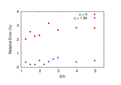
Figure 3: The relative error in LCM prediction for the two different lattice constant $c$ for various anode-cathode distance $D$.

The apex field enhancement factor can be determined with Eqns (9) and (6)-(8) for each value of $D$ and $c$. All emitters within a radius of $80c$ have been included while the number of images considered is typically around 1000. The apex field enhancement has also been computed using the finite element software COMSOL. The results are shown in Fig. 2.

Clearly, at the smaller nearest-neighbour pin spacings, the anode-proximity effect is much stronger using_COMSOL . To see this, note that $\gamma_{a}(D=1.25h,c=h)\simeq 330$ while $\gamma_{a}(D=10h,c=h)\simeq 226$ as compared to $\gamma_{a}(D=1.25h,c=1.5h)\simeq 337$ and $\gamma_{a}(D=10h,c=1.5h)\simeq 275$. Thus, as compared to $D=10h$, $\gamma_{a}$ increases by about $46\%$ at $D=1.25h$ for $c=h$, while over the same range, $\gamma_{a}$ increases by $22.5\%$ for $c=1.5h$. The effect is even more dramatic for $c=0.75h$ where $\gamma_{a}$ increases by $70\%$ with $\gamma_{a}(D=10h,c=0.75h)\simeq 185$ and $\gamma_{a}(D=1.25h,c=0.75h)\simeq 315.3$.

We next study the predictions of line charge model. It is obvious from Figs. 2 that the error is much smaller at larger nearest-neighbour pin spacings. This is quantified in Fig. 3 where the relative error defined as

$$\text{Relative Error}(\%)=\frac{\gamma_{a}^{comsol}(D,c)-\gamma_{a}^{LCM}(D,c)}{\gamma_{a}^{comsol}(D,c)}\times 100$$ (10)

is plotted. Here $\gamma_{a}^{comsol}(D,c)$ and $\gamma_{a}^{LCM}(D,c)$ are respectively the values of the apex field enhancement determined using COMSOL and LCM. For $c=1.5h$, the average error in prediction in the range $D=1.25h$ to $D=10h$ is about $0.43\%$ while for $c=h$, the average error increases to about $2.45\%$ in the same range of $D$. At $c=0.75h$, the average error increases to about $7\%$ for $D\in[1.25h,10h]$ with errors about $5\%$ for $D\in[1.25h,2h]$.

Thus, the line charge model captures the anode-proximity for arrays of emitters with errors that are generally below $2.5\%$ for $c\geq h$. It can thus be used to calculate the optimal spacing in the new light of enhanced anode-proximity effect for arrays of emitters. Recall that when the anode is at infinity db_rudra , the array current density is maximum when the lattice constant (or mean spacing) is about $2h$, with a slight variation depending on the electric field. In the presence of the anode, this optimal spacing is expected to change depending on the anode-cathode distance $D$.

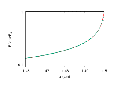
Figure 4: Variation of the electric field on the emitter surface around the apex follows the generalized cosine law $E(z,\rho)/E_{a}=\cos\tilde{\theta}=(z/h)/\sqrt{(z/h)^{2}+(\rho/R_{a})^{2}}$. The electric field data is obtained using COMSOL (solid curve) while the solid squares are obtained using the expression for $\cos\tilde{\theta}$. Here $D=1.25h$ and $c=h$.

For an infinite square lattice, the array current density $J_{array}$ is evaluated by calculating the current from a single emitter pin and dividing by $c^{2}$. Thus, $J_{array}=I_{pin}/c^{2}$ wheredb_distrib

$$I_{pin} \simeq 2\pi R_{a}^{2}{\cal G}J(0,h)$$ (11)

$$J(0,h) = \frac{1}{({t_{F}})^{2}}\frac{A_{\small{\rm FN}}}{W}E_{a}^{2}\exp(-B_{\small{\rm FN}}v_{{\small F}}W^{3/2}/E_{a})$$ (12)

where ${\cal G}=1/({\cal B}D_{1})$, $f_{0}\simeq 1.439965E_{a}/W^{2}$, $D_{1}=1-f_{0}/6$, $v_{\small F}=1-f_{0}+(1/6)f_{0}\ln f_{0}$, $t_{\small F}=1+f_{0}/9-(1/18)f_{0}\ln f_{0}$ and $E_{a}=\gamma_{a}(D,c)E_{0}$. In the above $W$ is the work-function (eV) and $A_{\small{\rm FN}}~{}\simeq~{}1.541434~{}{\rm\mu A~{}eV~{}V}^{-2}$ and $B_{\small{\rm FN}}~{}\simeq~{}6.830890~{}{\rm eV}^{-3/2}~{}{\rm V~{}nm}^{-1}$ are the conventional Fowler-Nordheim constantsFN ; Nordheim ; murphy ; forbes ; jensen_ency . The expression for ${\cal G}$ is obtained using the generalized cosine lawdb_ultram ; cosine of field variation near the apex, a result found to be true in the present scenario as shown in Fig. 4.

Fig. 5 shows the array current density for 2 values of macroscopic electric field and 3 values of anode-cathode distance $D$. Clearly, as the anode comes closer to the emitter ($D$ decreases), the optimal spacing becomes smaller and the maximum current density itself increases at any given macroscopic field as evident from the figures. Further, at a higher macroscopic field, the shift to smaller optimal spacing is greater. At $E_{0}=30$MV/m for instance, the optimal spacing is $c\simeq 0.75h$, which is smaller than the height of the emitter. The significance of the anode-proximity effect in a LAFE can be judged by noting that when the anode is far away ($D=100h$), the maximal current density is $1.19\times 10^{3}\text{A/m}^{2}$ at $E_{0}=20$MV/m ($c/h=2.4$) while at $E_{0}=30$MV/m, the maximal current density is $1.65\times 10^{3}$ ($c/h=2.13$).

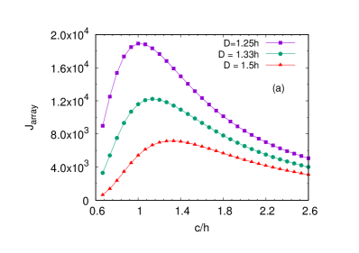
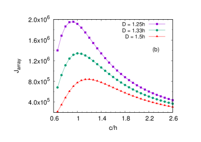
Figure 5: Variation of the array current density $J_{array}~{}({\rm A/m^{2}})$ with lattice spacing $c$ for 3 different anode-cathode spacing $D$ and (a) $E_{0}=20$MV/m and (b) $E_{0}=30$MV/m. Note that the optimal spacing shifts below the emitter height for $D=1.25h$ and $E_{0}=30$MV/m.

IV Discussions and Conclusions

It is clear from the preceding analysis that for a LAFE, the anode-proximity effect plays a dominant role and can counterbalance electrostatic shielding. We have also established that the line charge model predicts the apex field enhancement factor accurately for lattice constants $c\geq 1.5h$ while the error was found to be less than $5\%$ for $c=0.75h$ and anode distance $D\leq 2h$.

The line charge model in fact under-predicts the apex field enhancement factor $\gamma_{a}(D,c)$ for small values of $D$ and $c$. This is due to shape broadening of the zero-potential contour. The current densities obtained using LCM thus provide a lower bound.

In the present study, the dimensions of the emitter chosen are such that curvature-corrections to the tunneling potential are negligible (typically when $R_{a}>100$nm, see [db_curvature, ]). A similar analysis can be done for emitters with smaller apex radius of curvature (a few nanometers) using the curvature-corrected formula for emission currentdb_curvature ; db_gated . Due to the nature of the corrections db_curvature , it is easy to see that the current densities will decrease somewhat due to a slightly broadened tunneling barrier. Nevertheless, anode-proximity will play a dominant role and enhance the optimal current density. Note that though the emission current characteristics depend on the scale of the problem (e.g. nanometer vs micrometer), Eq. (9) is independent of the scale since the quantities involved are ratios of lengths and hence are dimensionless.

Finally, even though we have chosen an ellipsoid to demonstrate the enhanced anode-proximity effect in a LAFE, differently shaped emitters will also show the enhanced effect. The line charge model will also continue to hold but must be replaced by a nonlinear line-charge, making predictions slightly more involved db_anodeprox . The way forward seems to be semi-analytical model for non-ellipsoidal shapes where the prefactor of the logarithmic term in Eq. (9) and the ellipsoidal constant 2 are modified using numerical inputs such as in [db_anodeprox, ] while $\alpha_{A}$, $\alpha_{SA}$ and $\alpha_{S}$ are calculated analytically.

It is hoped that the results presented here will be useful in analysing LAFE emitter experiments or in designing cathodes. Of particular interest will be finite-sized array and a random distribution of emitters, both of which are presently beyond the reach of purely numerical methods. The finite array cannot be reliably analysed using finite element codes, especially ones that are small enough for surface effects to be important and yet too large for simulation. A random distribution consisting of few thousand emitters is another situation where the method described here can be used profitably. In both situations, the use of a gated-anode or a grid-anode in close proximity to the emitter-tips will lead to enhancement of the local field, compared to an anode that is far away. Experimental results on random LAFE such as in [bieker2018, ] where the emitter shape is conical and $D\simeq 2h$, offer a scope for validation of the model presented here.

V Acknowledgement

The authors wish to thank Gaurav Singh for valuable help and discussions.

 

VI References

References

- (1) C. A. Spindt, J. Appl. Phys., 39, 3504 (1968).
- (2) C. A. Spindt, C. E. Holland, A. Rosengreen and I. Brodie, IEEE Trans. on Electron Devices, 38, 2355 (1991).
- (3) K. B. K. Teo, E. Minoux, L. Hudanski, F. Peauger, J. P. Schnell, L. Gangloff, P. Legagneux, D. Dieumegard, G. .A.J. Amaratunga and W. I. Milne, Nature 437, 968 (2005).
- (4) Y. Li, Y. Sun and J. T. W. Yeow, Nanotechnology 26, 242001 (2015).
- (5) C. J. Edgcombe, Philos. Mag. B, 82, 1009 (2001).
- (6) R. G. Forbes, C.J. Edgcombe and U. Valdrè, Ultramicroscopy 95, 57 (2003).
- (7) F. H. Read and N. J. Bowring, Nucl. Instrum. Meth. Phys. Res. A 519, 305 (2004).
- (8) M. T. Cole, K. B. K. Teo, O. Groening, L. Gangloff, P. Legagneux, and W. I. Milne, Sci. Rep. 4, 4840 (2014).
- (9) A. I. Zhbanov, E. G. Pogorelov, Y.-C. Chang, and Y.-G. Lee, J. Appl. Phys. 110, 114311 (2011).
- (10) J. R. Harris, K. L. Jensen, D. A. Shiffler and J. J. Petillo, Appl. Phys. Lettrs. 106, 201603 (2015).
- (11) R. Forbes, J. App. Phys. 120, 054302 (2016).
- (12) D. Biswas and R. Rudra, Physics of Plasmas 25, 083105 (2018).
- (13) R. Rudra and D. Biswas, AIP Advances, 9, 125207 (2019).
- (14) X. Q. Wang, M. Wang, P. M. He, Y. B. Xu, and Z. H. Li, J. App. Phys, 96, 6752 (2004).
- (15) R. C. Smith, D. C. Cox and S. R. P. Silva, Appl. Phys. Lett. 87, 103112 (2005).
- (16) S. Podenok, M. Sveningsson, K. Hansen and E.E.B. Campbell, Nano 1, 87 (2006).
- (17) E.G. Pogorelov, A.I. Zhbanov, Y.-C. Chang, Ultramicroscopy 109 (2009) 373.
- (18) E. G. Pogorelov, Y-C. Chang, A. I. Zhbanov, and Y-G. Lee, J. App. Phys, 108, 044502 (2010).
- (19) D. Biswas, G. Singh and R. Kumar, J. App. Phys. 120, 124307 (2016).
- (20) S. Lenk, C. Lenk and I. W. Rangelow, J. Vac. Sci. Technol. B 36, 06JL01 (2018).
- (21) D. Biswas, Physics of Plasmas, 26, 073106 (2019).
- (22) The enhancement factors quoted here are obtained using COMSOL v5.4.
- (23) D. Biswas, Phys. Plasmas 25, 043113 (2018).
- (24) T. A. de Assis and F. F. Dall’Agnol, J. Vac. Sci. Tech. B, 37, 022902 (2019).
- (25) D. Biswas, Phys. Plasmas, 25, 043105 (2018).
- (26) R. H. Fowler and L. Nordheim, Proc. R. Soc. A 119, 173 (1928).
- (27) L. Nordheim, Proc. R. Soc. A 121, 626 (1928).
- (28) E. L. Murphy and R. H. Good, Phys. Rev. 102, 1464 (1956).
- (29) R. G. Forbes, App. Phys. Lett. 89, 113122 (2006).
- (30) K. L. Jensen, Field emission - fundamental theory to usage, Wiley Encycl. Electr. Electron. Eng. (2014).
- (31) D. Biswas, G. Singh, S. G. Sarkar and R. Kumar, Ultramicroscopy 185, 1 (2018).
- (32) D. Biswas, G. Singh and R. Ramachandran, Physica E 109, 179 (2019).
- (33) D. Biswas and R. Ramachandran, J. Vac. Sci. Technol. B 37, 021801 (2019).
- (34) D. Biswas and R. Kumar, J. Vac. Sci. Technol. B 37, 040603 (2019).
- (35) J. Bieker, F. Roustaie, and H. F. Schlaak, J. Vac. Sci. Technol. B 36, 02C105 (2018)