Contractivity of Runge-Kutta methods for convex gradient systems

Abstract

We consider the application of Runge-Kutta (RK) methods to gradient systems $(d/dt)x=-\nabla V(x)$, where, as in many optimization problems, $V$ is convex and $\nabla V$ (globally) Lipschitz-continuous with Lipschitz constant $L$. Solutions of this system behave contractively, i.e. the Euclidean distance between two solutions $x(t)$ and $\widetilde{x}(t)$ is a nonincreasing function of $t$. It is then of interest to investigate whether a similar contraction takes place, at least for suitably small step sizes $h$, for the discrete solution. Dahlquist and Jeltsch results’ imply that (1) there are explicit RK schemes that behave contractively whenever $Lh$ is below a scheme-dependent constant and (2) Euler’s rule is optimal in this regard. We prove however, by explicit construction of a convex potential using ideas from robust control theory, that there exists RK schemes that fail to behave contractively for any choice of the time-step $h$.

1 Introduction

Systems of differential equations

$$\frac{d}{dt}x=F(x),$$ (1.1)

with the gradient structure

$$\frac{d}{dt}x=-\nabla V(x),$$ (1.2)

arise in many applications and, accordingly, have attracted the interest of numerical analysts for a long time, see e.g. [1, 2] among many others. Here $V$ is a continuously differentiable real function defined in $\mathbb{R}^{d}$; in optimization applications $V$ is the objective function and in Physics problems corresponds to a potential. Since $(d/dt)V(x(t))\leq 0$, $V$ decreases along solutions. Furthermore, if $\lim_{t\rightarrow\infty}x(t)=x^{\star}$, then $x^{\star}$ is a stationary point of $V$, i.e., $\nabla V(x^{\star})=0$. These facts explain the well-known connections between numerical integrators for (1.2) and algorithms for the minimization of $V$. The simplest example is provided by the Euler integrator, that gives rise to the gradient descent optimization algorithm [3]. In the case where $\nabla V$ possesses a global Lipschitz constant $L>0$ and (1.2) is integrated with an arbitrary Runge-Kutta (RK) method, Humphries and Stuart [1] showed that the value of $V$ decreases along the computed solution, i.e. $V(x_{n+1})\leq V(x_{n})$, for positive stepsizes $h$ with $h\leq h_{0}$, where $h_{0}>0$ only depends on $L$ and on the RK scheme.

In view of the important role that convex objective functions play in optimization theory, see e.g. [3, Section 2.1.2], it is certainly of interest to study numerical integrators for (1.2) in the specific case where $V$ is convex, i.e.,

$$\forall x,y,\qquad\langle\nabla V(x)-\nabla V(y),x-y\rangle\geq 0$$ (1.3)

($\langle\cdot,\cdot\rangle$ and $\|\cdot\|$ stand throughout for the Euclidean inner product and norm in $\mathbb{R}^{d}$). After recalling (see [4, Section IV.2] or [5, Definition 112A]) that a system of the general form (1.1) is said to have one-sided Lipschitz constant $\nu$ if

$$\forall x,y,\qquad\langle F(x)-F(y),x-y\rangle\leq\nu\|x-y\|^{2},$$ (1.4)

we conclude that, for convex gradient systems (1.2), $\nu=0$. It follows that, for any two solutions $x(t)$, $\widetilde{x}(t)$ of a gradient system, we have the contractivity estimate

$$\forall t\geq 0,\qquad\|\widetilde{x}(t)-x(t)\|\leq\|\widetilde{x}(0)-x(0)\|,$$ (1.5)

and in particular for any solution $x(t)$ and any stationary point $x^{\star}$ (which by convexity will automatically be a minimizer)

$$\forall t\geq 0,\qquad\|x(t)-x^{\star}\|\leq\|x(0)-x^{\star}\|.$$

The study of linear multistep methods that, when applied to systems of the general form (1.1) with one-sided Lipschitz constant $\nu=0$, mimic the contractive behaviour in (1.5) began with the pioneering work of Dahlquist [6]. The corresponding results in the Runge-Kutta (RK) field followed immediately [7]. Those developments gave rise to the notions of algebraic stability/B-stability of RK methods (see [4, Section IV.12], [5, Section 357] and the monograph [8]) and G-stability of multistep methods ([4, Section V.6] or [5, Section 45]). These notions extend the concepts of A-stability [9] to a nonlinear setting. Of course, algebraically stable/B-stable RK schemes and G-stable multistep methods have to be implicit and therefore are not well suited to be the basis of optimization algorithms for large problems.

In this article we focus on the application of RK methods to gradient systems (1.2) where $V$ is convex and $\nabla V$ is Lipschitz continuous with Lipschitz constant $L$, i.e.

$$\forall x,y,\qquad\|\nabla V(x)-\nabla V(y)\|\leq L\|x-y\|,$$

or, in optimization terminology, where the objective function is convex and $L$-smooth. For our purposes here, we shall say that an interval $(0,h_{c}]$, $h_{c}=h_{c}(L)$, is an interval of convex contractivity of a given RK scheme if, for $h\in(0,h_{c}]$, any $L$-smooth convex $V$, and any two initial points $x_{0}$, $\widetilde{x}_{0}$, the corresponding RK solutions after one time step satisfy

$$\|\widetilde{x}_{1}-x_{1}\|\leq\|\widetilde{x}_{0}-x_{0}\|.$$ (1.6)

By analogy with the result by Humphries and Stuart quoted above, one may perhaps expect that each (consistent) Runge-Kutta method would possess an interval of convex contractivity; however this is not true. We establish in Section 3 that the familiar second-order method due to Runge that for the general system (1.1) takes the form

$$y_{1}=y_{0}+hF\Big{(}y_{0}+\frac{h}{2}F(y_{0})\Big{)}$$ (1.7)

possesses no interval of convex contractivity. The proof proceeds in two stages. We first follow the approach in [10, 11], based on ideas from robust control theory, and identify, for given $h$ and $L$, initial points $x_{0}$, $\widetilde{x}_{0}$ and gradient values

$$\nabla V(x_{0}),\quad\nabla V(\widetilde{x}_{0}),\quad\nabla V\Big{(}x_{0}-\frac{h}{2}\nabla V(x_{0})\Big{)},\quad\nabla V\Big{(}\widetilde{x}_{0}-\frac{h}{2}\nabla V(\widetilde{x}_{0})\Big{)}$$

that ensure that (1.6) is violated. In the second stage we provide a counterexample by constructing a suitable $L$-smooth $V$ by convex interpolation; this is not an easy task because multivariate convex interpolation problems with scattered data are difficult to handle [12, 13]. In order not to stop the flow of the paper, some proofs and technical details have been postponed to the final Sections 4 and 5.

For general systems (1.1), Dahlquist and Jeltsch [14] considered in an unpublished report (summarized in [8, Chapter 6]) the monotonicity requirement

$$\forall x,y,\qquad\langle F(x)-F(y),x-y\rangle\leq-\alpha\|F(x)-F(y)\|^{2},$$ (1.8)

that should be compared with (1.4). Under this requirement, they provided a characterization sufficient and necessary condition) for contractivity of non-confluent Runge–Kutta methods in the setting of equations $\dot{x}=F(t,x)$ satisfying the monotonicity condition (1.8). Since it is well known [3, Theorem 2.1.5] that $V$ is convex and $L$-smooth if and only if

$$\forall x,y,\qquad\frac{1}{L}\|\nabla V(x)-\nabla V(y)\|^{2}\leq\langle\nabla V(x)-\nabla V(y),x-y\rangle,$$ (1.9)

it turns out that convex, L-smooth gradient systems (1.2) satisfy (1.8) with $\alpha=1/L$ and the Dahlquist-Jeltsch result may be used to derive sufficient conditions for contractivity in our context; in particular it is possible for some explicit RK schemes to have nonempty intervals of convex contractivity. Similar time-step restrictions for explicit RK methods appear when instead of contractivity one is seeking to preserve monotonicity [15]. For completeness we present in Section 2 a version of the theorem by Dahlquist and Jeltsch tailored to our setting of $L$-smooth gradient systems. Dahlquist and Jeltsch also proved an opitimality property of Euler’s rule among explicit methods and we provide a new proof of their result. Optimality of methods of higher order was studied in [16].

Before closing the introduction we point out that there has been much recent interest [17, 18, 19, 20] in interpreting optimization algorithms as discretizations of differential equations (not necessarily of the form (1.2)), among other things because differential equations help to gain intuition on the behaviour of discrete algorithms.

2 Sufficient conditions for contractivity

The application of the $s$-stage RK method with coefficients $a_{ij}$ and weights $b_{j}$, $i,j=1,\dots,s$, to the system of differential equations (1.2) results in the relations

$$x_{1} = x_{0}+h\sum_{j=1}^{s}b_{j}k_{j},$$ (2.1)

$$X_{i} = x_{0}+h\sum_{j=1}^{s}a_{ij}k_{j},\quad i=1,\dots,s,$$

$$k_{j} = -\nabla V(X_{j}),\quad j=1,\dots,s.$$

Here the $X_{i}$ and $k_{i}$ are the stage vectors and slopes respectively. Of course, the scheme is consistent/convergent provided that $\sum_{j}b_{j}=1$.

Item 1 in the Theorem below is essentially Theorem 4.1 in [14] and holds for general systems (1.1) that satisfy (1.8) with $\alpha=1/L$ (in fact the proof presented below applies to that more general setting). The $s\times s$ symmetric matrix with entries

$$m_{ij}=b_{i}a_{ij}+b_{j}a_{ji}-b_{i}b_{j}$$

that appears in the hypotheses plays a central role in the study of algebraic stability as defined by Burrage and Butcher, [4, Definition 12.5] or [5, Definition 357B] and also in symplectic integration [21].

Theorem 2.1.

Let the scheme (2.1) be applied to the gradient system (1.2) with convex, $L$-smooth $V$.

Assume that:

1. The weights $b_{j}$, $j=1,\dots,s$, are nonnegative.

2. The $s\times s$ symmetric matrix $\overline{M}(h)$ with entries

   $$\overline{m}_{ij}(h)=\frac{2hb_{i}}{L}\delta_{ij}+h^{2}m_{ij}$$

   ($\delta$ is Kronecker’s symbol) is positive semidefinite.

Then:

1. If $x_{1}$ and $\widetilde{x}_{1}$ are the RK solutions after a step of lenght $h>0$ starting from $x_{0}$ and $\widetilde{x}_{0}$ respectively the contractivity estimate (1.6) holds.

2. In particular, if $x^{\star}$ is a minimizer of $V$, then

   $$\|x_{1}-x^{\star}\|\leq\|x_{0}-x^{\star}\|.$$

Proof. We start from the identity [4, Theorem 12.4]

$$\|\widetilde{x}_{1}-x_{1}\|^{2}=\|\widetilde{x}_{0}-x_{0}\|^{2}+2h\sum_{i=1}^{s}b_{i}\langle\widetilde{k}_{i}-k_{i},\widetilde{X}_{i}-X_{i}\rangle-h^{2}\sum_{i,j=1}^{s}m_{ij}\langle\widetilde{k}_{i}-k_{i},\widetilde{k}_{j}-k_{j}\rangle,$$

where $\widetilde{X}_{i}$ and $\widetilde{k}_{i}$ respectively denote the stage vectors and slopes for the step $\widetilde{x}_{0}\mapsto\widetilde{x}_{1}$. (This identity holds if $\langle\cdot,\cdot\rangle$ and $\|\cdot\|$ are replaced by any symmetric bilinear map and the associated quadratic map respectively, see [21, Lemma 2.5].) From (1.9), for $i=1,\dots,s$,

$$\langle\widetilde{k}_{i}-k_{i},\widetilde{X}_{i}-X_{i}\rangle\leq-\frac{1}{L}\langle\widetilde{k}_{i}-k_{i},\widetilde{k}_{i}-k_{i}\rangle,$$

which implies, in view of the nonnegativity of the weights,

$$\|\widetilde{x}_{1}-x_{1}\|^{2}\leq\|\widetilde{x}_{0}-x_{0}\|^{2}-\sum_{i,j=1}^{s}\overline{m}_{ij}(h)\langle\widetilde{k}_{i}-k_{i},\widetilde{k}_{j}-k_{j}\rangle.$$

If $\overline{M}(h)$ is positive semidefinite the sum is $\geq 0$ and the proof is complete. In addition, if we now set $\widetilde{x}_{0}=x^{\star}$, we trivially obtain $\|x_{1}-x^{\star}\|\leq\|x_{0}-x^{\star}\|$.

We next present some examples; the interested reader may find a full discussion in the report [14]. Hereafter $Q\succeq 0$ means that the matrix $Q$ is positive semidefinite.

Example 1. For Euler’s rule, $s=1$, $a_{11}=0$, $b_{1}=1$, we find $\overline{M}(h)=2h/L-h^{2}$ and therefore we have contractivity for $h$ in the interval $(0,2/L]$. This happens to coincide with the familiar stability interval for the linear scalar test equation $(d/dt)x=-Lx$, $L>0$. The restriction $h\leq 2/L$ on the step size is well known in the analysis of the gradient descent algorithm, see e.g. [3]. Observe that the scalar test equation arises from the $L$-smooth convex potential $V=Lx^{2}/2$ and that therefore no RK scheme can have an interval of convex contractivity longer than its linear stability interval.

Example 2. The formula two-stage, second order (1.7) presented in the introduction has $b_{1}=0$, $b_{2}=1$ and $a_{21}=1/2$. Thus

$$\overline{M}(h)=\left[\begin{matrix}0&\frac{h^{2}}{2}\\ \frac{h^{2}}{2}&\frac{2h}{L}-h^{2}\end{matrix}\right].$$

There is no value of $h>0$ for which this matrix is $\succeq 0$. In Theorem 3.3 we shall show that the scheme has no interval of convex contractivity. Hence for this RK method the sufficient condition in Theorem 2.1 is actually necessary. Note the necessity, under the requirement (1.8), of the hypotheses of Theorem 4.1 in [14] was not discussed by Dahlquist and Jeltsch.

Example 3. Explicit, two-stage, first-order scheme with $b_{1}=b_{2}=1/2$ and $a_{21}=1/2$. Here

$$\overline{M}(h)=\left[\begin{matrix}\frac{h}{L}-\frac{h^{2}}{4}&0\\ 0&\frac{h}{L}-\frac{h^{2}}{4}\end{matrix},\right]$$

and we have contractivity for $0<h\leq 4/L$. This could have been concluded from Example 1, because performing one step with this method yields the same result as taking two steps of length $h/2$ with Euler’s rule and accordingly, for this method, $h/2\leq 2/L$ ensures contractivity.

Example 4. We may generalize as follows. Consider the explicit $s$-stage, first-order scheme with Butcher tableau

$$\begin{matrix}0&0&0&\cdots&0\\ b_{1}&0&0&\cdots&0\\ b_{1}&b_{2}&0&\cdots&0\\ \vdots&\vdots&\vdots&\vdots&\vdots\\ b_{1}&b_{2}&b_{3}&\cdots&0\\ \hline\cr b_{1}&b_{2}&b_{3}&\cdots&b_{s}\end{matrix}$$ (2.2)

(i.e., $a_{ij}=b_{j}$ whenever $i>j$) with

$$\sum_{i=1}^{s}b_{i}=1,\qquad b_{i}\geq 0,\quad i=1,\dots,s.$$

Performing one step with this scheme is equivalent to successively performing $s$ steps with Euler’s rule with step-sizes $b_{1}h$, …, $b_{s}h$, and therefore contractivity is ensured in the case when $h\max_{i}b_{i}\leq 2/L$. This conclusion may alternatively be reached by applying Theorem 2.1; the method has $\overline{M}(h)$ given by

$${\rm diag}\big{(}2hb_{1}/L-h^{2}b_{1}^{2},\quad 2hb_{2}/L-h^{2}b_{2}^{2},\>\dots,\>2hb_{s}/L-h^{2}b_{s}^{2}\big{)},$$ (2.3)

a matrix that is $\succeq 0$ if and only if $h\max_{i}b_{i}\leq 2/L$. If we see the weights as parameters, then the least severe restriction on $h$ is attained by choosing equal weights $b_{i}=1/s$, $i=1,\dots,s$, leading to the condition $h\leq 2s/L$. But then one is really time-stepping with Euler rule with stepsize $h/s$.

Recall that RK schemes are called reducible if they give the same numerical results as a scheme with fewer stages; reducible methods are then completely devoid of interest. It is not difficult to prove (see [14, Corollary 3.4]) that RK schemes that are not reducible and for which $\overline{M}(h)\succeq 0$ for at least one value of $h$ have all its weights strictly positive. It is also known that irreuducible, explicit methods with positive weights have order $\leq 4$, [14, Theorem 4.4].

The next result is essentially Theorem 5.1 in [14] and shows that among explicit methods Euler’s rule has the longest interval of convex contractivity if intervals are scaled in terms of the number of stages so as to take the amount of work per step. Our purely algebraic proof is different from the analytic one given by Dahlquist and Jeltsch. Note that, in view of the comment we just made, the weights are assumed to be $>0$.

Theorem 2.2.

Consider an $s$-stage, explicit, consistent RK method with weights $>0$.

1. If for some $h>0$, $\overline{M}(h)\succeq 0$, then $h\leq 2s/L$.

2. If for $h=2s/L$, $\overline{M}(h)\succeq 0$, then the method is necessarily given by (2.2) with $b_{i}=1/s$, $i=1,\dots,s$ (i.e., it is the concatenation of $s$ Euler substeps of equal length $h/s$).

Proof. For the first item, we first note that, as we saw in Example 4, the result is true for the particular case where the scheme is of the form (2.2), i.e., a concatenation of Euler’s substeps. Let $\overline{M}_{\star}(h)$ be the matrix associated with the scheme of the form (2.2) that possesses the same weights as the given scheme (recall that this matrix was computed in (2.3)). The first item will be proved if we show that $\overline{M}(h)\succeq 0$ implies $\overline{M}_{*}(h)\succeq 0$, because, as we have just noted, the last condition guarantees that $h\leq 2s/L$. Assume that $\overline{M}(h)\succeq 0$. Then, its diagonal entries must be nonnegative,

$$0\leq\overline{m}_{ii}(h)=2hb_{i}/L-h^{2}b_{i}^{2},\qquad i=1,\dots,s,$$

and, in view of (2.3), this entails that $\overline{M}_{\star}(h)\succeq 0$, as we wanted to establish.

We now prove the second part of the theorem. If $\overline{M}(2s/L)\succeq 0$, then

$$0\leq\overline{m}_{ii}(2s/L)=4sb_{i}/L^{2}-4s^{2}b_{i}^{2}/L^{2},\qquad i=1,\dots,s,$$

or, after dividing by $4b_{i}s^{2}/L^{2}>0$, $b_{i}\leq 1/s$. Since $\sum_{i=1}^{s}b_{i}=1$, we conclude that $b_{i}=1/s$, $i=1,\dots,s$, which leads to $\overline{m}_{ii}(2s/L)=0$ for each $i$. A semidefinite positive matrix with vanishing diagonal elements must be the null matrix and therefore for $i>j$

$$0=\overline{m}_{ij}(2s/L)=(2s/L)^{2}(b_{i}a_{ij}-b_{i}b_{j})$$

and then $a_{ij}=b_{j}$. The proof is now complete.

3 An RK scheme without convex contractivity interval

In this section we show that the RK scheme (1.7) has no interval of convex contractivity.

For the system (1.2), we write the formulas for performing one step from the initial points $x_{0}$ and $\widetilde{x}_{0}$ in $\mathbb{R}^{d}$ as

$$x_{1}=x_{0}+hk_{h},\quad\widetilde{x}_{1}=\widetilde{x}_{0}+h\widetilde{k}_{h},\quad x_{h}=x_{0}+{\color[rgb]{0,0,0}\frac{h}{2}}k_{0},\quad\widetilde{x}_{h}=\widetilde{x}_{0}+\frac{h}{2}\widetilde{k}_{0},$$ (3.1)

with

$$k_{0}=-\nabla V(x_{0}),\quad\widetilde{k}_{0}=-\nabla V(\widetilde{x}_{0}),\quad k_{h}=-\nabla V(x_{h}),\quad\widetilde{k}_{h}=-\nabla V(\widetilde{x}_{h})$$ (3.2)

(the subindices $0$, $1$, $h$ refer to the beginning of the step, $t=0$, the end of the step, $t=h$, and the halfway location, $t=h/2$, respectively). Following the approach in [10, 11], we regard $x_{0}$, $\widetilde{x}_{0}$, $k_{0}$, $\widetilde{k}_{0}$, $k_{h}$, $\widetilde{k}_{h}$, as inputs, and $x_{0}$, $\widetilde{x}_{0}$, $x_{h}$, $x_{h}$, $x_{1}$, $\widetilde{x}_{1}$ as outputs. The relations (3.2) provide a feedback loop that expresses the inputs $k_{0}$, $\widetilde{k}_{0}$, $k_{h}$, $\widetilde{k}_{h}$ as values of a nonlinear function $\phi=-\nabla V$ computed at the outputs $x_{0}$, $\widetilde{x}_{0}$, $x_{h}$, $\widetilde{x}_{h}$. The function $\phi$ that establishes this feedback is the negative gradient of some $V$ that is convex and $L$-smooth. According to (1.9), this implies that the vectors $k_{0}$, $\widetilde{k}_{0}$, $k_{h}$, $\widetilde{k}_{h}$ delivered by the feedback loop must obey the following constraints:

$$\frac{1}{L}\|\widetilde{k}_{0}-k_{0}\|^{2} \leq -\langle\widetilde{k}_{0}-k_{0},\widetilde{x}_{0}-x_{0}\rangle,$$ (3.3)

$$\frac{1}{L}\|\widetilde{k}_{h}-k_{h}\|^{2} \leq -\langle\widetilde{k}_{h}-k_{h},\widetilde{x}_{h}-x_{h}\rangle,$$ (3.4)

$$\frac{1}{L}\|k_{h}-k_{0}\|^{2} \leq -\langle k_{h}-k_{0},x_{h}-x_{0}\rangle,$$ (3.5)

$$\frac{1}{L}\|\widetilde{k}_{h}-\widetilde{k}_{0}\|^{2} \leq -\langle\widetilde{k}_{h}-\widetilde{k}_{0},\widetilde{x}_{h}-\widetilde{x}_{0}\rangle,$$ (3.6)

$$\frac{1}{L}\|\widetilde{k}_{h}-k_{0}\|^{2} \leq -\langle\widetilde{k}_{h}-k_{0},\widetilde{x}_{h}-x_{0}\rangle,$$ (3.7)

$$\frac{1}{L}\|k_{h}-\widetilde{k}_{0}\|^{2} \leq -\langle k_{h}-\widetilde{k}_{0},x_{h}-\widetilde{x}_{0}\rangle$$ (3.8)

(we are dealing with four gradient values and therefore (1.9) may be applied in ${4\choose 2}=6$ ways). In a robust control approach, we will not assume at this stage that the vectors $k$ are values of one and the same function $-\nabla V$, on the contrary the vectors $k$ are seen as arbitrary except for the above constraints. More precisely, for fixed $L$ and $h$, we investigate the lack of contractivity by studying the real function

$$\frac{\|\widetilde{x}_{1}-x_{1}\|^{2}}{\|\widetilde{x}_{0}-x_{0}\|^{2}}$$ (3.9)

of the input variables $x_{0}$, $\widetilde{x}_{0}$, $k_{0}$, $\widetilde{k}_{0}$, $k_{h}$, $\widetilde{k}_{h}$, subject to the constraints $\widetilde{x}_{0}\neq x_{0}$ and (3.3)–(3.8). Here $x_{h}$, $x_{h}$, $x_{1}$, $\widetilde{x}_{1}$ are known linear combinations of the inputs given in (3.1).

Our task is made easier by the following observations. First of all, multiplication of $x_{0}$, $\widetilde{x}_{0}$, $x_{h}$, $\widetilde{x}_{h}$, $x_{1}$, $\widetilde{x}_{1}$, $k_{0}$, $\widetilde{k}_{0}$, $k_{h}$, $\widetilde{k}_{h}$ by the same scalar $\lambda>0$ preserves the relations (3.1), the constraints (3.3)–(3.8) and the value of the quotient (3.9). Therefore we may assume at the outset that $\|\widetilde{x}_{0}-x_{0}\|=1$. In addition, since the problem is also invariant by translations and rotations in $\mathbb{R}^{d}$, we may set $x_{0}=0\in\mathbb{R}^{d}$ and $\widetilde{x}_{0}=[1,0,0,\dots,0]^{T}$. After these simplifications, we are left with the task of ascertaining if we can make $\|\widetilde{x}_{1}-x_{1}\|^{2}$ larger than $1$ by choosing appropriately the vectors $k_{0}$, $\widetilde{k}_{0}$, $k_{h}$, $\widetilde{k}_{h}$ subject to the constraints. Here is a choice in $\mathbb{R}^{2}$ that works (see Section 4 for the origin of these vectors)

$$k_{0} = [0,-3/h]^{T},$$ (3.10)

$$\widetilde{k}_{0} = [-L/2,-3/h+L/2]^{T},$$ (3.11)

$$k_{h} = [0,-3/h+L]^{T},\quad$$ (3.12)

$$\widetilde{k}_{h} = [L^{3}h^{2}/64,-3/h+L-L^{2}h/8]^{T}.$$ (3.13)

In fact, with

$$x_{0}=[0,0]^{T},\qquad\widetilde{x}_{0}=[1,0]^{T}$$ (3.14)

and (3.10)–(3.13), the relations (3.1) yield

$$x_{h} = [0,-3/2]^{T},$$ (3.15)

$$\widetilde{x}_{h} = [1-Lh/4,-3/2+Lh/4]^{T},$$ (3.16)

$$x_{1} = [0,-3+Lh]^{T},$$ (3.17)

$$\widetilde{x}_{1} = [1+L^{3}h^{3}/64,-3+Lh+L^{2}h^{2}/8]^{T}.$$ (3.18)

It is a simple exercise to check that the constraints are satisfied at least for $Lh\leq 3$. In addition

$$\widetilde{x}_{1}-x_{1}=[1+L^{3}h^{3}/64,L^{2}h^{2}/8]^{T}$$

and, accordingly,

$$\|\widetilde{x}_{1}-x_{1}\|^{2}=1+\frac{1}{32}L^{3}h^{3}+\frac{1}{64}L^{4}h^{4}+\frac{1}{4096}L^{6}h^{6}>1=\|\widetilde{x}_{0}-x_{0}\|^{2}.$$ (3.19)

(The third power in $h^{3}$ matches the size of the local error of the scheme.)

Remark 3.1.

The vectors (3.10)–(3.13) become longer as $h$ decreases. This is a consequence of the way we addressed the study of (3.9) where we fixed the length of $\widetilde{x}_{0}-x_{0}$ for mathematical convenience. As pointed out above we could alternatively have chosen $x_{0}=[0,0]^{T}$, $\widetilde{x}_{0}=[h,0]^{T}$ and multiplied (3.10)–(3.13) by a factor of $h$ and that would have given a configuration with bounded gradients resulting in lack of contractivity.

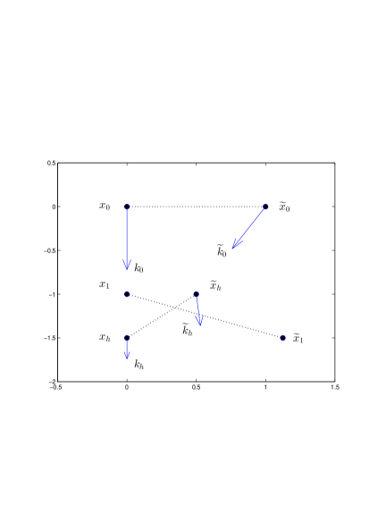
Figure 1: A configuration that satisfies the constraints resulting from convexity and $L$-smoothness and leads to lack of contractivity for $L=2$, $h=1$

To get some insight, we have depicted in Figure 1, when $L=2$, $h=1$, the points $x_{0}$, $\widetilde{x}_{0}$, $x_{h}$, $\widetilde{x}_{h}$, $x_{1}$, $\widetilde{x}_{1}$ along with the vectors $k_{0}$, $\widetilde{k}_{0}$, $k_{h}$, $\widetilde{k}_{h}$ (for clarity, the vectors have been drawn after multiplying their length by $0.8$). The difference vector $\widetilde{k}_{0}-k_{0}$ forms, as required by convexity, an obtuse angle with $\widetilde{x}_{0}-x_{0}$ and this causes $\widetilde{x}_{h}-x_{h}=\widetilde{x}_{0}-x_{0}+(h/2)(\widetilde{k}_{0}-k_{0})$ to be shorter than $\widetilde{x}_{0}-x_{0}$. Similarly the difference $\widetilde{k}_{h}-k_{h}$ forms by convexity an obtuse angle with $\widetilde{x}_{h}-x_{h}$ and if $x_{1}$ and $\widetilde{x}_{1}$ were alternatively defined as $x_{h}+(h/2)k_{h}$ and $\widetilde{x}_{h}+(h/2)\widetilde{k}_{h}$ respectively we see from the Figure that we would have $\|\widetilde{x}_{1}-x_{1}\|\leq\|\widetilde{x}_{0}-x_{0}\|$. (That alternative time stepping was studied in Example 3 in the preceding section.) However for our RK scheme (1.7) the direction of $k_{h}$ is used to displace $x_{0}$ (rather than $x_{h}$) to get $x_{1}$ (and similarly for the points with tilde); the vector $\widetilde{k}_{h}-k_{h}$ forms an acute angle with $\widetilde{x}_{0}-x_{0}$ and this makes it possible for $\widetilde{x}_{1}-x_{1}$ to be longer than $\widetilde{x}_{0}-x_{0}$. For smaller values of $L$ and/or $h$ the effect is not so marked as that displayed in the figure but is nevertheless present.

While (3.19) is consistent with the scheme having no interval of convex contractivity, we are not yet done, because it is not obvious whether there is a convex, $L$-smooth $V$ that realizes the relations (3.2) for the $x$’s and $k$’s we have found. Nevertheless the preceding material will provide the basis for proving in the final section the following result:

Theorem 3.3.

Fix $L>0$. For the RK scheme (1.7) and each arbitrarily small value of $h>0$, there exist an $L$-smooth, convex $V$ and initial points $x_{0}$ and $\widetilde{x}_{0}$ such that (1.6) is not satisfied. As a consequence the scheme does not possess an interval of convex contractivity.

One could perhaps say that the method has an empty interval of convex contractivity.

4 The construction of the auxiliary gradients

The proof of Theorem 3.3 hinges on the use of the vectors (3.10)–(3.13). In this section we briefly describe how we constructed them.

Let us introduce the vectors in $\mathbb{R}^{2}$

$$\delta_{0}=\widetilde{x}_{0}-x_{0},\qquad\delta_{h}=\widetilde{x}_{h}-x_{h},\qquad\delta_{1}=\widetilde{x}_{1}-x_{1}$$

and

$$\Delta_{0}=\widetilde{k}_{0}-k_{0},\qquad\Delta_{h}=\widetilde{k}_{h}-k_{h},$$

so that $\delta_{1}=\delta_{0}+h\Delta_{h}$ and $\delta_{h}=\delta_{0}+(h/2)\Delta_{0}$. We fixed $\delta_{0}=[1,0]^{T}$ as explained in Section 3, saw $\Delta_{0}$ and $\Delta_{h}$ as variables in $\mathbb{R}^{2}$ and considered the problem of maximizing $\|\delta_{1}\|^{2}$ under the constraints (3.3)–(3.4), i.e

$$\frac{1}{L}\|\Delta_{0}\|^{2}\leq-\langle\Delta_{0},\delta_{0}\rangle,\qquad\frac{1}{L}\|\Delta_{h}\|^{2}\leq-\langle\Delta_{h},\delta_{h}\rangle,$$

With some patience, we solved this maximization problem analytically in closed form after introducing Lagrange multipliers. Both constraints are active at the solution. The expression of the maximizer is a complicated function of $L$ and $h$ and to simplify the subsequent algebra we expanded that expression in powers of $h$ and kept the leading terms. This resulted in

$$\Delta_{0}=[-L/2,L/2]^{T},\qquad\Delta_{h}=[L^{3}h^{2}/64,-L^{2}h/8]^{T}$$

(there is a second solution obtained by reflecting this with respect to the first coordinate axis).

Once we had found candidates for the differences $\widetilde{k}_{0}-k_{0}$, $\widetilde{k}_{h}-k_{h}$, we identified suitable candidates for $k_{0}$ and $k_{h}$. We arbitrarily fixed the direction of $k_{0}$ by choosing it to be perpendicular to $\delta_{0}$ (see (3.10)). Its second component was sought in the form $c/h$ ($c$ a constant) so that the distance between $x_{h}$ and $x_{0}$ behaved like $\mathcal{O}(1)$ as $h\downarrow 1$ (recall that we have scaled things in such a way that $\widetilde{x}_{0}$ and $x_{0}$ are also at a distance $\mathcal{O}(1)$ as $h\downarrow 1$). We also took $k_{h}$ to be perpendicular to $\delta_{0}$; the second component of this vector was chosen to be of the form $c/h-c^{\prime}L$ so as to have $k_{h}-k_{0}=-c^{\prime}L$ with a view to satisfying (3.5). After some numerical experimentation we saw that the values $c=3$, $c^{\prime}=1$ led to a set of vectors for which all six contraints (3.3)–(3.8) hold at least for $Lh\leq 3$.

For the sake of curiosity we also carried out numerically the maximization of (3.9) subject to the constraints. It turns out that the maximum value of the quotient is approximately $1+0.032L^{3}h^{3}$ for $h$ small, independently of the dimension $d\geq 2$ of the problem (for $d=1$ the experiments suggest that the scheme is contractive). Since, in (3.19), $1/32=0.03125$ the vectors (3.10)–(3.13) are very close to providing the combination of gradients that leads to the greatest dilation (3.9).

5 Proof of Theorem 3.3

The proof proceeds in two stages. We first construct an auxiliary piecewise linear, convex ${\color[rgb]{0,0,0}\widetilde{V}}$ and then we regularize it to obtain $V$.

5.1 Constructing a piecewise linear potential by convex interpolation

Let $L>0$ be the Lispchitz constant and set ${L^{\prime}}=\alpha L$, where $\alpha$ is a positive safety factor, independent of $L$ and $h$, whose value will be determined later. Restrict hereafter the attention to values of $h$ with $h{L^{\prime}}\leq 1$. We wish to construct a potential ${\color[rgb]{0,0,0}\widetilde{V}}$ for which the application of the RK scheme starting from the two initial conditions (3.14) lead to the relations (3.10)–(3.13), (3.15)–(3.18) with ${L^{\prime}}$ in lieu of $L$ and therefore, as we know, to lack of contractivity.

We consider the following four (pairwise distinct) points in the plane $\mathbb{R}^{2}$ of the variable $\zeta$ (see (3.15)–(3.18))

$$Z_{1} = [0,0]^{T},$$

$$Z_{2} = [1,0]^{T},$$

$$Z_{3} = [0,-3/2]^{T},$$

$$Z_{4} = [1-{L^{\prime}}h/4,-3/2+{L^{\prime}}h/4]^{T},$$

and associate with them the four (pairwise distinct) vectors (see (3.10)–(3.13))

$${\color[rgb]{0,0,0}G_{1}} = [0,3/h]^{T},$$

$${\color[rgb]{0,0,0}G_{2}} = [{L^{\prime}}/2,3/h-{L^{\prime}}/2]^{T},$$

$${\color[rgb]{0,0,0}G_{3}} = [0,3/h-{L^{\prime}}]^{T},\quad$$

$${\color[rgb]{0,0,0}G_{4}} = [-{L^{\prime}}^{3}h^{2}/64,3/h-{L^{\prime}}+{L^{\prime}}^{2}h/8]^{T},$$

and four real numbers $F_{i}$ that will be determined below. We then pose the following Hermite convex interpolation problem: Find a real convex function ${\color[rgb]{0,0,0}\widetilde{V}}$ defined in $\mathbb{R}^{2}$, differentiable in the neighbourhood of the $Z_{i}$, and such that

$${\color[rgb]{0,0,0}\widetilde{V}}(Z_{i})=F_{i},\qquad\nabla{\color[rgb]{0,0,0}\widetilde{V}}(Z_{i})=G_{i},\qquad i=1,\dots,4.$$

If the interpolation problem has a solution, then the tangent plane to $\eta={\color[rgb]{0,0,0}\widetilde{V}}(\zeta)$ at $Z_{i}$ is given by the equation $\eta=\pi_{i}(\zeta)$ with

$${\color[rgb]{0,0,0}\pi_{i}(\zeta)}\ =F_{i}+\langle G_{i},\zeta-Z_{i}\rangle,\qquad i=1,\dots,4.$$

and, by convexity,

$$F_{i}\geq\pi_{j}(Z_{i}),\qquad i\neq j,\quad i,j=1,\dots,4.$$ (5.1)

This is then a necessary condition for the Hermite problem to have a solution. We found the following set of values

$$F_{1} = 0,$$

$$F_{2} = \frac{{L^{\prime}}}{4},$$

$$F_{3} = -\frac{9}{2h}+\frac{9{L^{\prime}}}{8},$$

$$F_{4} = -\frac{9}{2h}+\frac{15{L^{\prime}}}{8}-\frac{{L^{\prime}}^{2}h}{4}+\frac{{L^{\prime}}^{3}h^{2}}{128},$$

that satisfy the relations (5.1) (in fact they satisfy all of them with strict inequality).

It is not difficult to see [12, 13], that once we have ensured (5.1), the Hermite problem is solvable. The solution is not unique and among all solutions the minimal is clearly given by the piecewise linear function

$${\color[rgb]{0,0,0}\widetilde{V}}(\zeta)=\max\{\pi_{i}(\zeta):i=1,\dots,4\}.$$

From Section 3 we conclude that, if the RK scheme is applied to solve the gradient system associated with ${\color[rgb]{0,0,0}\widetilde{V}}$ with starting points $x_{0}=Z_{1}$, $\widetilde{x}_{0}=Z_{2}$, then (3.19) holds with $L$ replaced by ${L^{\prime}}$ and there is no contractivity. However, the proof is not complete because ${\color[rgb]{0,0,0}\widetilde{V}}$ is not continuously differentiable (let alone $L$-smooth). Accordingly we shall regularize ${\color[rgb]{0,0,0}\widetilde{V}}$ to construct the potential $V$ we need.

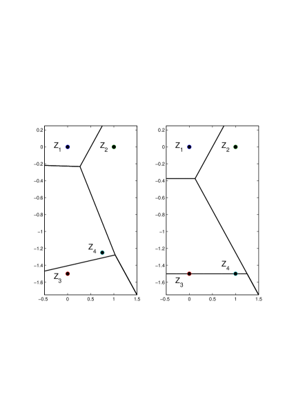
Figure 2: Left: points $Z_{i}$ and tessellation associated with the piecewise linear convex interpolant when ${L^{\prime}}h=1$. Right: points $Z_{i}$ and tessellation in the limit ${L^{\prime}}h\downarrow 0$

Before we do so, it is convenient to notice that ${\color[rgb]{0,0,0}\widetilde{V}}$ gives rise to four closed, convex regions [12, 13]

$${\cal R}_{i}=\{\zeta:{\color[rgb]{0,0,0}\widetilde{V}}(\zeta)=\pi_{i}(\zeta)\},\quad i=1,\dots,4,$$

that tessellate the plane. Clearly $Z_{i}\in{\cal R}_{i}$, $i=1,\dots,4$. The equations of the lines that bound the regions are of course found by intersecting the planes $\eta=\pi_{i}(\zeta)$, $i=1,\dots,4$. After carrying out the corresponding trite computations, it turns out that those boundaries depend on $h$ and ${L^{\prime}}$ only through the product ${L^{\prime}}h$. (By the way, the same is true of the coordinates of the points $Z_{i}$.) For ${L^{\prime}}h=1$, the maximum value under consideration of the product ${L^{\prime}}h$, we have depicted the interpolation nodes and regions in the left panel of Figure 2. Note that the gradient $\nabla{\color[rgb]{0,0,0}\widetilde{V}}$ takes the constant value $G_{i}$ in the interior of the region ${\cal R}_{i}$. This gradient is then discontinuous at the boundaries of the tessellation; from the analytic expressions for the $G_{i}$ we see that the jumps $\|G_{i}-G_{j}\|$ at the boundaries may be bounded above by $C_{1}{L^{\prime}}$ with $C_{1}$ a constant independent of ${L^{\prime}}$ and $h$.

While the interpolation problem above only makes sense for positive $h$, the points $Z_{i}$ and the tessellation have well-defined limits as $h\downarrow 0$; these limits are depicted in the right panel of Figure 2. Note for future reference that, in the limit, $Z_{3}$ and $Z_{4}$ are on the common boundary of ${\cal R}_{3}$ and ${\cal R}_{4}$.

5.2 Regularization by convolution

For $\zeta\in\mathbb{R}^{2}$ let us denote by ${\cal S}(\zeta)\subset\mathbb{R}^{2}$ the closed square centered at $\zeta$ with side $\ell/2$ (i.e. the closed $L_{\infty}$-ball centered at $\zeta$ with radius $\ell/2$)). The regularization procedure uses the real-valued function $\chi(\zeta)$ such that $\chi(\zeta)=1/\ell^{2}$ if $\zeta\in{\cal S}(0)$ and $\chi(\zeta)=0$ if $\zeta\notin{\cal S}(0)$. Clearly $\int_{\mathbb{R}^{2}}\chi(\zeta)\,d\zeta=1$.

We fix the value of $\ell$ in such a way that for all ${L^{\prime}}>0$ and all $h\leq 1/{L^{\prime}}$ (see Figure 2)

$${\cal S}(Z_{1})\subset{\cal R}_{1},\quad{\cal S}(Z_{2})\subset{\cal R}_{2},\quad{\cal S}(Z_{3})\subset{\cal R}_{3}\cup{\cal R}_{4},\quad{\cal S}(Z_{4})\subset{\cal R}_{3}\cup{\cal R}_{4};$$

it is not possible to achieve ${\cal S}(Z_{3})\subset{\cal R}_{3}$, or ${\cal S}(Z_{4})\subset{\cal R}_{4}$ because $\ell$ is not allowed to depend on $h$ and, as $h$ decreases, $Z_{3}$ and $Z_{4}$ approach the boundary of ${\cal R}_{3}$ and ${\cal R}_{4}$, as we just pointed out.

We define the regularized potential by the convolution

$$V(\zeta)=\int_{\mathbb{R}^{2}}\chi(\zeta^{\prime})\,{\color[rgb]{0,0,0}\widetilde{V}}(\zeta-\zeta^{\prime})\,d\zeta^{\prime}.$$

Each translated function $\zeta\mapsto{\color[rgb]{0,0,0}\widetilde{V}}(\zeta-\zeta^{\prime})$ is convex and $\chi(\zeta^{\prime})\geq 0$ so that $V$ is convex, as a convex combination of convex functions. Furthermore

$$\nabla V(\zeta)=\int_{\mathbb{R}^{2}}\chi(\zeta^{\prime})\,\nabla{\color[rgb]{0,0,0}\widetilde{V}}(\zeta-\zeta^{\prime})\,d\zeta^{\prime}$$

(the integrand is not defined on the lines that define the tessellation) or

$$\nabla V(\zeta)=\int_{\mathbb{R}^{2}}\chi(\zeta-\zeta^{\prime})\,\nabla{\color[rgb]{0,0,0}\widetilde{V}}(\zeta^{\prime})\,d\zeta^{\prime}=\frac{1}{\ell^{2}}\int_{\{\zeta^{\prime}\in{\cal S}(\zeta)\}}\nabla{\color[rgb]{0,0,0}\widetilde{V}}(\zeta^{\prime})\,d\zeta^{\prime}.$$

Since $\zeta^{\prime}\mapsto\nabla{\color[rgb]{0,0,0}\widetilde{V}}(\zeta^{\prime})$ is piecewise constant with value $G_{i}$ in the interior of ${\cal R}_{i}$, $i=1,\dots,4$, for each fixed $\zeta$, the vector $\nabla V(\zeta)$ is a convex linear combination of the vectors $G_{i}$, $i=1,\dots,4$, and the weights of this combination are given by $(1/\ell^{2})$ times the areas of the intersections ${\cal S}(\zeta)\cap{\cal R}_{i}$. This shows that $\nabla V$ is a continuous function (i.e. that $V$ is continuous differentiable). In addition, if for a given location $\zeta$ the square ${\cal S}(\zeta)$ is entirely contained in one of the regions ${\cal R}_{i_{0}}$, then $\nabla V(\zeta)=G_{i_{0}}$. By our choice of $\ell$ it follows that

$$\nabla V(Z_{1})=G_{1},\qquad\nabla V(Z_{2})=G_{2}.$$ (5.2)

The geometric interpretation of the definition of $\nabla V(\zeta)$ also shows that $\nabla V$ is Lipschitz continuous with a Lipschitz constant of the form $C_{2}D/\ell$, where $D$ is an upper bound for the size of the jumps $\|G_{i}-G_{j}\|$, $i,j=1,\dots,4$. As remarked earlier, $D=C_{1}{L^{\prime}}$, so that $\nabla V$ is is Lipschitz continuous with Lipschitz constant $C_{1}C_{2}{L^{\prime}}/\ell$. Therefore by choosing our safety factor as $\alpha=\ell/(C_{1}C_{2})$, the potential $V$ will be convex and $L$-smooth.

Finally take RK solutions for the problem (1.2) from the poins $x_{0}=Z_{1}$ and $\widetilde{x}_{0}=Z_{2}$. From (5.2) and the definition of $G_{1}$ and $G_{2}$, we have $x_{h}=Z_{3}$ and $\widetilde{x}_{h}=Z_{4}$. Next

$$\nabla V(x_{h})=\nabla V(Z_{3})=\lambda G_{3}+(1-\lambda)G_{4},$$

$$\nabla V(\widetilde{x}_{h})=\nabla V(Z_{4})=(1-\mu)G_{3}+\mu G_{4}$$

where $\lambda$ is $1/\ell^{2}$ times the area of ${\cal S}(Z_{3})\cap{\cal R}_{3}$ and $\mu$ is $1/\ell^{2}$ times the area of ${\cal S}(Z_{4})\cap{\cal R}_{4}$. We observe that $\lambda>1/2$ for $h>0$ because ${\cal S}(Z_{3})\cup{\cal R}_{3}$ clearly has more area than ${\cal S}(Z_{3})\cup{\cal R}_{4}$. Similarly $\mu>1/2$ for $h>0$. The quantities $\lambda$ and $\mu$ depend on ${L^{\prime}}$ and $h$ and approach $1/2$ as $h\downarrow 0$. We then find

$$\widetilde{x}_{1}-x_{1}=[1+\nu{L^{\prime}}^{3}h^{3}/64,-\nu{L^{\prime}}^{2}h^{2}/8]^{T},\qquad\nu=\mu-(1-\lambda)>0$$

and

$$\|\widetilde{x}_{1}-x_{1}\|^{2}=1+\frac{1}{32}\nu{L^{\prime}}^{3}h^{3}+\frac{1}{64}\nu^{2}{L^{\prime}}^{4}h^{4}+\frac{1}{4096}\nu^{2}{L^{\prime}}^{6}h^{6}>1.$$

This estimate is worse than (3.19) due to the presence of ${L^{\prime}}$ and $\nu$, but still sufficient to prove the theorem. By using functions $\chi$ smoother than the one we used above, it is possible to construct by convolution smoother potentials $V$. However, our choice here results in a clearer proof.

Acknowledgements. J.M.S. was supported by project MTM2016-77660-P(AEI/ FEDER, UE) funded by MINECO (Spain). He would like to thank the Isaac Newton Institute for Mathematical Sciences for support and hospitality during the programme “Geometry, compatibility and structure preservation in computational differential equations” when work on this paper was undertaken. This work was supported by EPSRC Grant Number EP/R014604/1. K.C.Z was supported by the Alan Turing Institute under the EPSRC grant EP/N510129/1. The authors are also thankful to J. Carnicer (Zaragoza) for bringing to their attention a number of helpful references on convex interpolation.

References

- [1] A.R. Humphries and A.M. Stuart. Runge-Kutta methods for disspative and gradient dynamical systems. SIAM J. Num. Anal., 31:1452–1485, 1994.
- [2] E. Hairer and C. Lubich. Energy-diminishing integration of gradient systems. IMA J. Numer. Anal., 34:452–461, 2014.
- [3] Y. Nesterov. Introductory Lectures on Convex Optimization: A Basic Course. Springer Publishing Company, Incorporated, 1 edition, 2014.
- [4] Ernst Hairer and Gerhard Wanner. Solving ordinary differential equations II. Stiff and differential-algebraic problems. Springer-Verlag, Berlin and Heidelberg, 1996.
- [5] J. C. Butcher. Numerical methods for ordinary differential equations. John Wiley & Sons, Ltd., Chichester, third edition, 2016. With a foreword by J. M. Sanz-Serna.
- [6] G. G. Dahlquist. Error analysis for a class of methods for stiff non-linear initial value problems. In G. Alistair Watson, editor, Numerical Analysis, pages 60–72, Berlin, Heidelberg, 1976. Springer Berlin Heidelberg.
- [7] J. C. Butcher. A stability property of implicit runge-kutta methods. BIT Numerical Mathematics, 15(4):358–361, Dec 1975.
- [8] K. Dekker and J. G. Verwer. Stability of Runge-Kutta methods for stiff nonlinear differential equations, volume 2 of CWI Monographs. North-Holland Publishing Co., Amsterdam, 1984.
- [9] G. G. Dahlquist. A special stability problem for linear multistep methods. BIT Numerical Mathematics, 3(1):27–43, Mar 1963.
- [10] L. Lessard, B. Recht, and A. Packard. Analysis and design of optimization algorithms via integral quadratic constraints. SIAM Journal on Optimization, 26(1):57–95, 2016.
- [11] Mahyar Fazlyab, Alejandro Ribeiro, Manfred Morari, and Victor M. Preciado. Analysis of optimization algorithms via integral quadratic constraints: nonstrongly convex problems. SIAM J. Optim., 28(3):2654–2689, 2018.
- [12] J. M. Carnicer. Multivariate convexity preserving interpolation by smooth functions. Adv. Comput. Math., 3(4):395–404, 1995.
- [13] J. M. Carnicer and M. S. Floater. Piecewise linear interpolants to Lagrange and Hermite convex scattered data. Numer. Algorithms, 13(3-4):345–364 (1997), 1996.
- [14] G. Dahlquist and R. Jeltsch. Generalized disks of contractivity for explicit and implicit Runge-Kutta methods. 1979.
- [15] Inmaculada Higueras. Monotonicity for Runge–Kutta methods: Inner product norms. Journal of Scientific Computing, 24(1):97–117, Jul 2005.
- [16] J. F. B. M. Kraaijevanger. Contractivity of Runge-Kutta methods. BIT Numerical Mathematics, 31(3):482–528, Sep 1991.
- [17] M. J. Ehrhardt, E. S. Riis, T. Ringholm, and C.-B. Schönlieb. A geometric integration approach to smooth optimisation: Foundations of the discrete gradient method, 2018.
- [18] D. Scieur, V. Roulet, F. R. Bach, and A. d’Aspremont. Integration methods and optimization algorithms. In Advances in Neural Information Processing Systems 30: Annual Conference on Neural Information Processing Systems 2017, 4-9 December 2017, Long Beach, CA, USA, pages 1109–1118, 2017.
- [19] W. Su, S. Boyd, and E. J. Candès. A differential equation for modeling Nesterov’s accelerated gradient method: Theory and insights. Journal of Machine Learning Research, 17(153):1–43, 2016.
- [20] A. Wibisono, A. C. Wilson, and M. I. Jordan. A variational perspective on accelerated methods in optimization. Proceedings of the National Academy of Sciences, 113(47):E7351–E7358, 2016.
- [21] J. M. Sanz-Serna. Symplectic Runge-Kutta schemes for adjoint equations, automatic differentiation, optimal control, and more. SIAM Rev., 58(1):3–33, 2016.