Classification in asymmetric spaces via sample compression

Abstract

We initiate the rigorous study of classification in quasi-metric spaces. These are point sets endowed with a distance function that is non-negative and also satisfies the triangle inequality, but is asymmetric. We develop and refine a learning algorithm for quasi-metrics based on sample compression and nearest neighbor, and prove that it has favorable statistical properties.

Keywords: Classification, quasi-metrics.

We initiate the rigorous study of classification in quasi-metrics. These are spaces endowed with a distance function that is non-negative, obeys the triangle inequality, but not symmetric. The term ‘quasi-metric’ appears as early as Wilson (1936), and it has been the subject of significant research in such areas as topology (Künzi, 2001) and theoretical computer science. As pointed out by Lawvere (1973), quasi-metrics occur naturally in many settings and applications, such as directed graphs and Hausdorff distances on certain subsets of metric space. More simply, travel times on road networks are quasi-metrics (due for example to traffic and one-way streets), as are travel times on uneven terrain, since marching up to the top of a hill takes more time than marching down again. For this reason, there has been significant work addressing the Travelling Salesman Problem in asymmetric spaces (Frieze et al., 1982; Asadpour et al., 2010; Anari and Gharan, 2015; Svensson et al., 2017).

Turing to classification, if we wish to classify in quasi-metric spaces – for example, determine whether an unknown village belongs to one country or another, based on its proximity to known villages – we require classification tools that are resilient to asymmetry. In general, we inhabit an inherently asymmetric world, yet we are unaware of any rigorous study of learning in quasi-metric spaces. Indeed, much of the existing machinery for classification algorithms, as well as generalization bounds, depend strongly on the axioms of the metric spaces, and so do not immediately transfer over to quasi-metric space. Our goal in this paper is to introduce techniques, tools, and statistical analysis for learning in this setting, for which no classification guarantees were previously known.

Our task is aided by a preexisting framework for learning in metric spaces of low intrinsic dimensionality. (Luxburg and Bousquet, 2004; Gottlieb et al., 2014a; Kontorovich and Weiss, 2014). In these spaces, it is known that a small sample is sufficient to achieve classification with low generalization error via the nearest neighbor classifier. It is also known that dependence on the dimensionality is unavoidable (Shalev-Shwartz and Ben-David, 2014). This framework proved sufficiently powerful to extend to non-metric space such as semi-metrics (which do not obey the triangle inequality), although this extension required developing a new definition of dimensionality (Gottlieb et al., 2017). We wish to use this framework as a foundation for learning in quasi-metrics as well, but the weak structure of quasi-metric make this a non-trivial task.

Our contribution.

We present a rigorous approach to learning in quasi-metric spaces. We define a new measure of dimensionality for quasi-metric spaces, and show how this measure can be used for sample compression (Section 2.1). We then present a classifier based on compression and proximity, and prove strong generalization bounds for it (Section 2.2). Our classification framework implies a range of new algorithmic questions which we address in Section 3. There we explore different approaches to sample compression for quasi-metrics, as well as prove the complexity of evaluation time for our classifier.

Finally, we turn to some simple metrization techniques for quasi-metrics, and show that while these techniques can transform the quasi-metric into metric or semi-metric spaces, the transformation typically induces a degradation in some property necessary for learning (dimension or margin), rendering this approach undersirable (Section 4).

Related work.

As mentioned, quasi-metric were a subject of mathematical study as early as the 1930’s (Wilson, 1936). Very early approaches to these spaces already attempted ‘metrization’ to transform them into the more malleable metric spaces (Frink, 1937), but more recently the very limited nature of this approach has been acknowledged (Schroeder, 2006; Dung et al., 2019). Other properties of quasi-metrics have been studied as well: For example, Stoltenberg (1969) considered the relationship between quasi-metrics and Moore spaces, with emphasis compactness and metrizability. (See also follow up work by Reilly (1976).) Doitchinov (1988) studied a notion of Cauchy sequences in quasi-metrics, while Goubault-Larrecq (2017) introduced and studied Lipschitz-regular quasi-metric spaces. Recently, Mémoli et al. (2018) studied generalizations of classical metric embeddings to the quasimetric setting, for example embedding quasi-metric spaces into ultra-quasi-metrics. and these have many algorithmic applications. We refer the reader to these papers for many additional references.

Quasi-metrics have also appeared in a number of machine learning applications. For example, Gutiérrez-Naranjo et al. (2002) introduced a quasi-metric operator, while others focused on computable analysis (Shao-Bai Chen et al., 2005) or optimization (Chen et al., 2006). The performance of nearest neighbor search under quasi-metric distance has also been studied (Klimo et al., 2018; Zhang et al., 2019), and Stojmirovic (2008) showed that similarity between peptides can be modeled via quasi-metrics. As previously stated, none of these present a rigorous classification framework for quasi-metrics.

1 Preliminaries

Notation and basic concepts.

We describe the recursive logarithm as $\log^{(1)}n=\log n$ and $\log^{(x)}n=\log\log^{(x-1)}n$ for $x>1$. For example, $\log^{(2)}n=\log\log n$ and so $\log^{(3)}n=\log\log\log n$, etc. The iterative logarithm $\log^{*}n$ is the smallest integer $i$ satisfying $\log^{(i)}n\leq 1$.

A $k$-hierachically well-separated tree ($k$-HST) (Bartal, 1996) has the property that in any root-to-leaf path in the tree, the edge lengths decrease by a factor of exactly $k$ in each step. See figure 1.

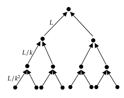
Figure 1: A $k$-HST with height 3.

Distance spaces.

A distance function $\rho:\mathcal{X}\times\mathcal{X}\rightarrow\mathbb{R}^{1}$ defines the distance between two points of the set $\mathcal{X}$. For two sets $A,B$, we define $\rho(A,B)=\min_{a\in A,b\in B}\rho(a,b)$. Likewise, $\rho(a,B)=\min_{b\in B}\rho(a,b)$.

A metric space $(\mathcal{X},\rho)$ is an instance space $\mathcal{X}$ endowed with a distance function $\rho$ that is non-negative, symmetric ($\rho(x,y)=\rho(y,x)\;\forall x,y\in\mathcal{X}$) and obeys the triangle inequality: $\rho(x,y)\leq\rho(x,z)+\rho(z,y)\;\forall x,y,z\in\mathcal{X}$. Often, one requires also that the distance function satisfy $\rho(x,y)=0\Leftrightarrow x=y$.

In a semi-metric space $(\mathcal{X},\rho)$, the distance function $\rho$ obeys the above metric conditions, with the exception of the triangle inequality. In quasi-metrics, the distance function obeys the above metric conditions, with the exception of only the symmetry property.

In all cases, the diameter of $\mathcal{X}$ is defined as $\operatorname{diam}(\mathcal{X})=\max_{x,y\in\mathcal{X}}\rho(x,y)$.

Balls and dimension.

For a metric or semi-metric space $(\mathcal{X},\rho)$, define ball $B_{r}(x)\subset\mathcal{X}$ to be all points of $\mathcal{X}$ within distance $r$ of some point $x$. Let $\lambda=\lambda(\mathcal{X},\rho)$ be the smallest value such that for every radius $r$ and center-point $x\in\mathcal{X}$, $B_{r}(x)$ can be covered by $\lambda$ balls of radius $\frac{r}{2}$. Then $\lambda$ is the doubling constant of $(\mathcal{X},\rho)$. The doubling dimension of $\mathcal{X}$ is defined as $\operatorname{ddim}(\mathcal{X},\rho)=\log_{2}\lambda(\mathcal{X},\rho)$ (Assouad, 1983; Gupta et al., 2003).

For a metric or semi-metric space $(\mathcal{X},\rho)$, the density constant $\mu=\mu(\mathcal{X},\rho)$ (Gottlieb and Krauthgamer, 2013) is the smallest number such that any $r$-radius ball in $\mathcal{X}$ contains at most $\mu$ points at mutual interpoint distance at least $r/2$: The density dimension of $\mathcal{X}$ is $\operatorname{dens}(\mathcal{X},\rho)=\log_{2}\mu(\mathcal{X},\rho)$.

A dimension property is called hereditary if it applies to all subspaces of the space of interest, that is if $\operatorname{prop}(\mathcal{X}^{\prime})\leq\operatorname{prop}(\mathcal{X})$ for all $\mathcal{X}^{\prime}\subset\mathcal{X}$. The doubling constant is known to to semi-hereditary in that $\lambda(\mathcal{X}^{\prime})\leq\lambda(\mathcal{X})^{2}$ for all $\mathcal{X}^{\prime}\subset\mathcal{X}$. The mild increase in the doubling constant is due to the fact that points that serve as the centers of covering balls of $\mathcal{X}$ may not be present in $\mathcal{X}$, necessitating the use of other centers which may not cover all points.

We note that the stated definition of balls – and therefore, of the doubling and density constants – assumed a symmetric distance function and therefore is ill-posed for the asymmetric distances of a quasi-metrics. Addressing this issue is a central component of this paper, see Section 2.

Samples and compression.

In a slight abuse of notation, we will blur the distinction between $S\subset\mathcal{X}$ as a collection of points in a quasimetric space and $S\in\mathcal{X}\times\{-1,1\})^{n}$ as a sequence of labeled examples. Thus, the notion of a sub-sample $\tilde{S}\subset S$ partitioned into its positively and negatively labeled subsets as $\tilde{S}=\tilde{S}_{+}\cup\tilde{S}_{-}$ is well-defined.

In metric and semi-metric spaces, one can condense the sample $S$ to a consistent subset $S^{\prime}\subset$ of sizes $\left(\frac{\operatorname{diam}}{\rho(S_{+},S_{-})}\right)^{O(\log\lambda(S,\rho))}$ and $\left(\frac{\operatorname{diam}}{\rho(S_{+},S_{-})}\right)^{O(\log\mu(S,\rho))}$, respectively. This means that for any $x\in S_{+}$ the nearest neighbor of $x$ in $S^{\prime}$ is some positively labelled point, while for any $x\in S_{-}$ the nearest neighbor of $x$ in $S^{\prime}$ is some negatively labelled point. It follows that a nearest-neighbor classifier using the condensed set $S^{\prime}$ correctly classifies all points of $S$.

Strong generalization bounds are known for classifiers via sample compression. For consistent classiers, we have:

Theorem 1 (Graepel et al. (2005))

For any distribution over $\mathcal{X}\times\left\{-1,1\right\}$, any $n\in\mathbb{N}$ and any $0<\delta<1$, with probability at least $1-\delta$ over the random sample $S$ of size $n$, the following holds: If hypothesis $h_{S}$ queries only a $k$-point subset $S^{\prime}\subset S$ (that is, $h_{S^{\prime}}(x)=h_{S}(x)$ for all $x\in\mathcal{X}$) then ${\displaystyle\operatorname{err}(h_{S})\leq\frac{1}{n-k}\left((k+1)\log n+\log\frac{1}{\delta}\right).}$

For classifiers with sample error, we have:

Theorem 2 (Gottlieb et al. (2017))

Fix a distribution over $\mathcal{X}\times\left\{-1,1\right\}$, an $n\in\mathbb{N}$ and $0<\delta<1$. With probability at least $1-\delta$ over the random sample $S$ of size $n$, the following holds for all $0\leq\epsilon\leq\frac{1}{2}$: If hypothesis $h_{S}$ queries only a $k$-point subset $S^{\prime}\subset S$ (that is, $h_{S^{\prime}}(x)=h_{S}(x)$ for all $x\in\mathcal{X}$) and misclassifies only an $\epsilon$ fraction of points in $S$, then putting $\tilde{\epsilon}={\epsilon n}/({n-d})$, we have

$$\operatorname{err}(h_{S}) \leq \tilde{\epsilon}+\frac{2}{3(n-k)}\log\frac{n^{k+1}}{\delta}+\sqrt{\frac{9\tilde{\epsilon}(1-\tilde{\epsilon})}{2(n-k)}\log\frac{n^{k+1}}{\delta}}$$ (1)

2 Dimension of quasi-metric spaces and learning

In metric spaces, the doubling dimensional is known to control the quality of learning via sample compression. We wish to apply the same approach for quasi-metrics, but here the doubling dimension is not well defined, since the classic definition of a ball assumes a symmetric space. This motivates us to define analogous notions of balls and dimensions in quasi-metrics, and apply them to learning.

2.1 Directional covering

Definition 3

For a quasi-metric $(\mathcal{X},\rho)$, define $B^{\operatorname{out}}_{r}(x)=\{y\in\mathcal{X}:\rho(x,y)\leq r\}$ and $B^{\operatorname{in}}_{r}(x)=\{y\in\mathcal{X}:\rho(y,x)\leq r\}$.

These two distinct notions of balls give rise to two distinct notions of covering constants:

Definition 4

For a quasi-metric $(\mathcal{X},\rho)$, let its outer-constant $\lambda^{\operatorname{out}}=\lambda^{\operatorname{out}}(\mathcal{X},\rho)$ be the smallest value such that for every radius $r$ and center-point $x\in\mathcal{X}$, $B^{\operatorname{out}}_{r}(x)$ can be covered by $\lambda^{\operatorname{out}}$ balls of the form $B^{\operatorname{out}}_{r/2}(y)$ (where $y\in\mathcal{X}$).

Likewise, let the inner-constant $\lambda^{\operatorname{in}}=\lambda^{\operatorname{in}}(\mathcal{X},\rho)$ be the smallest value such that for every radius $r$ and center-point $x\in\mathcal{X}$, $B^{\operatorname{in}}_{r}(x)$ can be covered by $\lambda^{\operatorname{in}}$ balls of the form $B^{\operatorname{in}}_{r/2}(y)$ (where $y\in\mathcal{X}$).

The definitions of outer-constant and inner-constant are closely related, and $\lambda^{\operatorname{out}},\lambda^{\operatorname{in}}$ can be interchanged by simply reflecting the distance funtion, that is swapping the values $\rho(x,y)$ and $\rho(y,x)$ for all $x,y\in\mathcal{X}$. Nevertheless, the value of the outer-constant and inner-constant of a single quasi-metric may be vastly different:

Lemma 5

There exists a quasi-metric $(\mathcal{X},\rho)$ for which $\lambda^{\operatorname{out}}=O(1)$ while $\lambda^{\operatorname{in}}=n$, and vice-versa.

Proof  Consider a directed graph $G=(V,E)$ with $n$ vertices $v_{1},\ldots,v_{n}\in V(G)$, where $E$ contains directed edges of length 1 connecting all pairs $v_{i},v_{i+1}$ ($1\leq i<n$), and directed edges of length $1$ connecting $v_{i}$ to $v_{1}$ for all $1<i\leq n$. (This graph is illustrated in Figure 2.)

Consider any ball of the form $B^{\operatorname{out}}_{r}(v_{i})$ (where $r\geq 1$); this ball contains the points $v_{j}$ for the two (possibly overlapping) ranges $j\in[i,\min\{i+r,n\}]$ and $j\in[1,\min\{r-1,n\}]$. The three points $v_{i},v_{i+\lceil r/2\rceil},v_{\lceil r/2\rceil-1}$ cover the two ranges. Now consider the ball $B^{\operatorname{in}}_{1}(v_{1})$ – this is a ball of radius 1 covering all points. Clearly, $n$ balls of the form $B^{\operatorname{in}}_{1/2}(v_{i})$ are required to cover the entire space.

The reverse claims follows trivially by reversing the direction of the edges.  

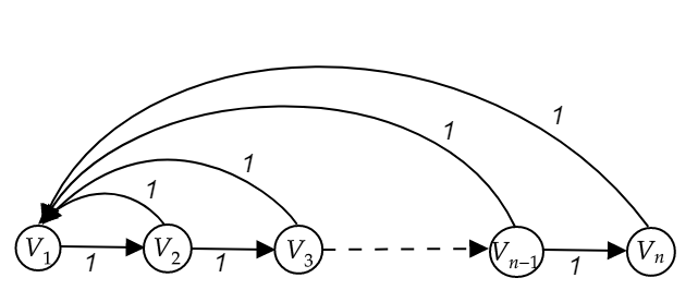
Figure 2: A directed graph with low inner-constant and high outer-constant

Having defined the outer- and inner-constants, we can show that each one can be used to bound the size of a set covering the space (Lemma 6), and by extension that learning is possible in quasi-metrics with bounded outer- or inner-constants (Theorem 7). This is parallel to the doubling constant controlling compression in metric spaces, and the density constant controlling compression in semi-metric spaces.

As usual, define the diameter of quasi-metric $(\mathcal{X},\rho)$ to be $\operatorname{diam}=\operatorname{diam}(\mathcal{X},\rho)=\max_{x,y\in\mathcal{X}}\rho(x,y)$. A subset $C\subset\mathcal{X}$ is called an $\alpha$-outer-cover for $\mathcal{X}$ if for all $x\in\mathcal{X}$ we have $\rho(C,x)\leq\alpha$. Likewise, a subset $C\subset\mathcal{X}$ is an $\alpha$-inner-cover for $\mathcal{X}$ if for all $x\in\mathcal{X}$ we have $\rho(x,C)\leq\alpha$. We can show the following:

Lemma 6

Let $(\mathcal{X},\rho)$ be a quasi-metric of diameter $\operatorname{diam}=\operatorname{diam}(\mathcal{X},\rho)$. Then $\mathcal{X}$ admits an outer-cover of size at most $(\lambda^{\operatorname{out}})^{\lceil\log(\operatorname{diam}/\alpha)\rceil}$, and an inner-cover of size at most $(\lambda^{\operatorname{in}})^{\lceil\log(\operatorname{diam}/\alpha)\rceil}$.

Proof  We prove the outer-cover claim, and proof of the inner-cover claim is similar: $\mathcal{X}$ can be covered by $\lambda^{\operatorname{out}}$ balls of the type $B^{\operatorname{out}}_{\operatorname{diam}/2}(x)$. Assign each point of $\mathcal{X}$ to its covering ball (or to one of its covering balls if it is covered by multiple balls.) Then each of these $\frac{\operatorname{diam}}{2}$-radius balls can be covered by $\lambda^{\operatorname{out}}$ balls of the type $B^{\operatorname{out}}_{\operatorname{diam}/4}(x)$. Continue this procedure recursively for a total of $\lceil\log(\operatorname{diam}/\alpha)\rceil$ steps until reaching balls of diameter at most $\alpha$. The centers of all balls of this radius constitute an $\alpha$-outer-cover with the claimed size.  

In the next section, we show that a small outer- or inner-cover can used for learning.

2.2 Learning via compression

Given a sample $S=S_{+}\cup S_{-}$ and distance function $\rho$ such that $(S,\rho)$ is a quasi-metric, we will utilize the outer- or inner- constant to produce a consistent classifier (that is a classifier with no sample error on $S$) and prove generalization bounds for it.

Consider the margin from all positive points to all negative points, $\rho^{\pm}=\rho(S_{+},S_{-})$. If we extract from $S_{+}$ a $\rho^{\pm}$-outer cover $C^{\pm}_{\operatorname{out}}\subset S_{+}$ of size $(\lambda^{\operatorname{out}}(S_{+},\rho))^{\lceil\log(\operatorname{diam}/\rho^{\pm})\rceil}$, then $\rho(C,x)\leq\rho^{\pm}$ for all $x\in S_{+}$, while $\rho(C,x)>\rho^{\pm}$ for all $x\in S_{-}$. So $C^{\pm}_{\operatorname{out}}$ can be used in a consistent classifier for $S$. Similarly, we may extract from from $S_{-}$ a $\rho^{\pm}$-inner cover $C^{\pm}_{\operatorname{in}}\subset S_{-}$ of size $(\lambda^{\operatorname{in}}(S_{-},\rho))^{\lceil\log(\operatorname{diam}/\rho^{\pm})\rceil}$, and then $\rho(x,C)>\rho^{\pm}$ for all $x\in S_{+}$, while $\rho(x,C)\leq\rho^{\pm}$ for all $x\in S_{-}$. So $C^{\pm}_{\operatorname{in}}$ can also be used in a consistent classifier for $S$.

We may also consider the margin from all negative points to all positive points, $\rho^{\mp}=\rho(S_{-},S_{+})$, and as above both an inner-cover of $S_{+}$ of size $(\lambda^{\operatorname{in}}(S_{+},\rho))^{\lceil\log(\operatorname{diam}/\rho^{\mp})\rceil}$ or an outer-cover of $S_{-}$ of size $(\lambda^{\operatorname{out}}(S_{-},\rho))^{\lceil\log(\operatorname{diam}/\rho^{\mp})\rceil}$ can be used to produce a consistent classifier. See Figure 3.

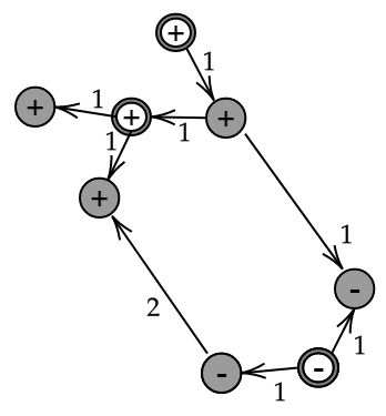
Figure 3: Outer covers and margins for $S_{+},S_{-}$. Here, $\rho^{\pm}=1$ and $\rho^{\mp}=2$.

Theorem 1 implies that the size of cover controls the generalization bounds of its associated classifier, and so of these four possible classifiers, we choose the cover of the smallest size. We conclude:

Theorem 7

For any $(\mathcal{X},\rho)$ forming a quasi-metric, any distribution over $\mathcal{X}\times\left\{-1,1\right\}$, any $n\in\mathbb{N}$ and any $0<\delta<1$, with probability at least $1-\delta$ over the random sample $S=S_{+}\cup S_{-}$ of size $n$, the following holds:

$${\displaystyle\operatorname{err}(h_{S})\leq\frac{1}{n-k}\left((k+1)\log n+\log\frac{1}{\delta}\right).}$$ (2)

where

$$k = \min\{(\lambda^{\operatorname{out}}(S_{+},\rho))^{\lceil\log(\operatorname{diam}/\rho^{\pm})\rceil},(\lambda^{\operatorname{in}}(S_{-},\rho))^{\lceil\log(\operatorname{diam}/\rho^{\pm})\rceil},$$

$$(\lambda^{\operatorname{in}}(S_{+},\rho))^{\lceil\log(\operatorname{diam}/\rho^{\mp})\rceil},(\lambda^{\operatorname{out}}(S_{-},\rho))^{\lceil\log(\operatorname{diam}/\rho^{\mp})\rceil}\}$$

Lemma 6 and Theorem 7 show how to learn quasi-metrics, but they do not touch upon the computational complexity and runtime associated with computing a cover or a classifier, nor of evaluating the classifier on a new point. These will be addressed in Section 3.

3 Computational complexity and algorithms

Here we address the computational issues arising from an implementation of the classifiers of Theorem 7. In Section 3.1, we address the problem of finding small $\alpha$-covers, and in Section 3.2 we show that evaluating the classifiers of Theorem 7 requires $\Theta(n)$ distance computations.

3.1 Computing a cover

Lemma 6 demonstrates that a space with small outer- or inner-constant admits a small outer- or inner-cover. But the proof is non-constructive, and indeed even in metric spaces finding an optimal cover is NP-hard, and also hard to approximate within some polynomial factor (Gottlieb et al., 2014b). In this section, we give three algorithms for producing outer- or inner-covers.

Greedy cover.

One possible approach to constructing an $\alpha$-cover (whether outer or inner) is the arbitrary algorithm: Choose a point $x\in S$ arbitrarily, add $x$ to the cover $C$, remove from $S$ all points $\alpha$-covered by $x$, and repeat. While this algorithm is close to the best possible for metric spaces (for sub-exponential time algorithms (Gottlieb et al., 2014b), we can show it is arbitrarily bad in quasi-metrics: Consider for example a 1-inner-cover for the directed line of Figure 4. The arbitrary algorithm may choose the first vertex ($v_{1}$ in the figure) – which inner-covers no other points – then the second and third, etc., until all points are placed in the cover.

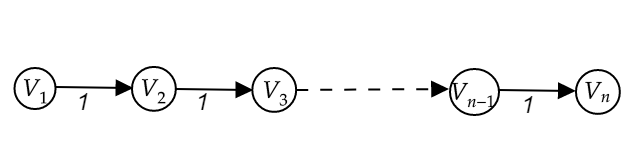
Figure 4: A directed line graph

However, we can show that a simple greedy algorithm gives a $\ln n$-approximation to the minimum cover. This algorithm simply chooses the point of $S$ that $\alpha$-covers the largest number of other points of $S$, removes all these points from $S$ and adds the covering point to $C$, and repeats until $S$ is empty. The greedy construction of an $\alpha$-inner-cover is given in Algorithm 1, and construction of an $\alpha$-outer-cover is similar.

Data: Sample $S$, parameter $\alpha$.

Result: $C\subset$ is an $\alpha$-inner-cover for $S$.

$A\leftarrow S$;

while $A\neq\emptyset$ do

       $x=\arg\max_{y\in S}\{|B^{\operatorname{in}}(y,\alpha)\cap A|\}$;

       $C\leftarrow C\cup\{x\}$;

       $A\leftarrow A\backslash B^{\operatorname{in}}(x,\alpha)$;

      

end while

return $C$

Algorithm 1 Greedy inner-cover construction

Lemma 8

Algorithm 1 returns an $\alpha$-cover $C$ with cardinality at most a $(\lceil\ln|S|\rceil+1)$-factor times the optimal cover. It can be implemented for quasi-metrics in time $O(n^{2})$.

Proof  Let $p$ be the size of the optimal cover. This implies that for any subset $S^{\prime}\subset S$, there is a point of $S$ that covers at least $\frac{|S^{\prime}|}{p}$ points of $S^{\prime}$. Then after $p\ln|S|$ iterations, the number of remaining points in $A$ is at most $|S|\left(1-\frac{1}{p}\right)^{p(\lceil\ln|S|\rceil+1)}\leq|S|e^{-\frac{1}{p}\cdot p(\lceil\ln|S|\rceil+1)}<1$, so all points are covered.

For the runtime, we initially compute for every point the set of points it covers, and then sort the points into buckets depending on the number of points they cover, in total time $O(n^{2}+n\log n)=O(n^{2})$. When a point is removed $A$, all points covering it must be updated and moved to the adjacent smaller bucket, a cost of $O(n)$ per removed point, for a total of $O(n^{2})$.  

It follows that a cover returned by Algorithm 1 can be used to create a classifier satisfying the bounds of Theorem 7, with the dependence on $k$ in Equation 2 replaced by a similar dependence on $k(\lceil\ln|S|\rceil+1)$.

Improved approximation.

The greedy algorithm gives an additional $\ln n$ factor in the size of the cover – that is total size at most $(\lambda^{\operatorname{in}})^{\log(\operatorname{diam}/\alpha)}\ln n$ – but this approximation factor may be undesirable. We can show that a better approximation factor can be attained by iteratively executing the greedy algorithm multiple times. Let $\alpha_{i}$ satisfy $(\lambda^{\operatorname{in}})^{\lceil\log(\operatorname{diam}/\alpha_{i})\rceil}=\log^{(i)}n$. Running the greedy algorithm with $\alpha_{1}$ produces an $\alpha_{1}$-inner-cover $C_{1}\subset S$ of size $O(\log^{2}n)$ (where for simplicity we have taken $\lambda^{\operatorname{in}}$ to be constant with respect to $n$). We then run the greedy algorithm to find an $\alpha_{2}$-inner-cover $C_{2}\subset S$ for $C_{1}$, of size $O(\log\log n\cdot\log C_{1})=O(\log^{2}\log n)$. Repeating this operation until reaching $j$ for which $\alpha_{j}\geq\frac{\alpha}{3}$ – that is, fewer than $\log^{*}n$ times – we eliminate the dependence on $n$, and replace it with a factor polynomial in the optimal $\alpha$-cover. It is easily verify that the set $C_{j-1}$ is of size at most $\exp\left((\lambda^{\operatorname{in}})^{O(\log(\operatorname{diam}/\alpha))}\right)$. See Algorithm 2 for a full description. From the above analysis we conclude:

Theorem 9

Algorithm 2 returns an $\alpha$-inner-cover of cardinality $(\lambda^{\operatorname{in}})^{O(\log(\operatorname{diam}/\alpha))}$, or an $\alpha$-outer-cover of cardinality $(\lambda^{\operatorname{out}})^{O(\log(\operatorname{diam}/\alpha))}$. It can be implemented for quasi-metrics in time $O(n^{2}\log^{*}n)$.

Data: Sample S, margin $\alpha$.

Result: $C$ is an $\alpha$-inner-net for $S$.

$i\leftarrow 1$;

$C\leftarrow S$;

while $\alpha_{i}<\alpha/3$ do

       $C\leftarrow$ Algorithm 3$(S,C,\alpha_{i})$;

       $i\leftarrow i+1$;

      

end while

$C\leftarrow$ Algorithm 3$(S,C,\alpha-\sum_{j=1}^{i-1}\alpha_{j})$;

return $C$

Algorithm 2 Improved $\alpha$-inner-cover construction ($\alpha_{i}$ is defined in the text)

Data: Sample $S$, subset $S^{\prime}$, parameter $\alpha$.

Result: $C\subset S$ is an $\alpha$-inner-cover for $S^{\prime}$.

$A\leftarrow S^{\prime}$;

while $A\neq\emptyset$ do

       $x=\arg\max_{y\in S}\{|B^{\operatorname{in}}(y,\alpha)\cap A|\}$;

       $C\leftarrow C\cup\{x\}$;

       $A\leftarrow A\backslash B^{\operatorname{in}}(x,\alpha)$;

      

end while

return $C$

Algorithm 3 Greedy cover subroutine

A cover returned by Algorithm 2 can be used to create a classifier satisfying the bounds of Theorem 7, with the dependence on $k$ in Equation 2 replaced by a similar dependence on $k^{O(1)}$.

Inconsistent cover.

The previous $\alpha$-cover algorithms required consistency, meaning that every point in $S_{+}$ or $S_{-}$ be $\alpha$-covered. However, Theorem 2 gives generalization bounds in the presence of errors. That is, even if a computed cover covers only a $(1-\epsilon)$ fraction of the points, the bounds of Theorem 2 hold with parameters $\epsilon$ and

$$k = \min\{(\lambda^{\operatorname{out}}(S_{+},\rho))^{\lceil\log(\operatorname{diam}/\rho^{\pm})\rceil},(\lambda^{\operatorname{in}}(S_{-},\rho))^{\lceil\log(\operatorname{diam}/\rho^{\pm})\rceil},$$

$$(\lambda^{\operatorname{in}}(S_{+},\rho))^{\lceil\log(\operatorname{diam}/\rho^{\mp})\rceil},(\lambda^{\operatorname{out}}(S_{-},\rho))^{\lceil\log(\operatorname{diam}/\rho^{\mp})\rceil}\}$$

To this end, we modify Algorithm 1 to take an additional parameter $\epsilon$, and to terminate when the working set is sufficiently small: In particular, we replace the condition ‘while $A\neq\emptyset$ do’ with ‘while $|A|>\epsilon|S|$ do’. This gives us the following lemma:

Lemma 10

The modified greedy algorithm returns an $\alpha$-cover with cardinality at most a $\lceil\ln(1/\epsilon)\rceil$-factor times optimal. The returned $\alpha$-cover covers at least a $(1-\epsilon)$-fraction of the points. It can be implemented for quasi-metrics in time $O(n^{2})$.

Proof  As in the proof of Lemma 8, let $p$ be the size of the optimal cover. This implies that for any subset $S^{\prime}\subset S$, there is a point of $S$ that covers at least $\frac{|S^{\prime}|}{p}$ points of $S^{\prime}$. Then after $p\lceil\ln(1/\epsilon)\rceil$ iterations, the number of remaining points in $A$ is at most $|S|\left(1-\frac{1}{p}\right)^{p(\lceil\ln(1/\epsilon)\rceil)}\leq|S|e^{-\frac{1}{p}\cdot p(\lceil\ln(1/\epsilon)\rceil)}\leq\epsilon|S|$.

The runtime of the modified greedy algorithm is the same as for the original greedy algorithm.  

A cover returned by the modified greedy algorithm can be used to create a classifier satisfying the bounds of Theorem 2, with the dependence on $k$ in Equation 1 replaced by a similar dependence on $k\lceil\ln(1/\epsilon)\rceil$, where $k$ is as above.

3.2 Nearest neighbor search

The classifier of Theorem 7 requires the evaluation of the distance of a query point to or from $S_{+}$ or $S_{-}$, which reduces to nearest neighbor search. Note that in doubling spaces, there exist $(1+\epsilon)$-approximate nearest neighbor search algorithms with fast run-time $\lambda^{O(1)}\log n+\lambda^{O(\log(1/\epsilon))}$ (Krauthgamer and Lee, ; Har-Peled and Mendel, 2006; Cole and Gottlieb, ), Thus, instead of constructing a classifier based on an $\alpha$-cover and then executing an exact nearest neighbor search to $S_{+}$ or $S_{-}$, one can instead construct a classifier based on a $\frac{\alpha}{2}$-cover, and execute a fast $2$-approximate nearest neighbor search, which will correctly classify the query point. However, we can show the situation for nearest neighbor search for quasi-metrics is significantly worse than for metrics:

Lemma 11

Let $(\mathcal{X},\rho)$ be a quasi-metric. There exists a subset $S$ for which an $(1+\epsilon)$-approximate nearest neighbor search minimizing $\rho(q,S)$ (respectively, $\rho(S,q)$) for $S$ and some $q\in\mathcal{X}$ may require $\theta(n)$ distance computations, even when $\lambda^{\operatorname{in}}(S,\rho)$ and $\lambda^{\operatorname{in}}(S\cup q,\rho)$ are constant (respectively, $\lambda^{\operatorname{out}}(S,\rho)$ and $\lambda^{\operatorname{out}}(S\cup q,\rho)$ are constant).

Proof  We prove the case of $\rho(q,S)$, and the case of $\rho(S,a)$ is similar. Consider the case where $S$ is a full binary $2$-HST with edges directed towards the root. The tree has depth $p$, and an edge connecting a node to its depth $i$ parent has length $2^{-i}$. The query possesses an infinitesimally small edge directed to a single leaf, no edges to any other leaf, and edges of length $\sum_{i=j}^{p-1}2^{-i}$ to all nodes of depth $j<p$. It is easily verified that both $\lambda^{\operatorname{in}}(S,\rho)$ and $\lambda^{\operatorname{in}}(S\cup q,\rho)$ are constant.

As the distance from $q$ to any $j$-level ($j<p$) point is the same, $q$ must be compared to all leaves to find its nearest neighbor, at a cost of $\Theta(n)$ comparisons.  

It follows that $\Theta(n)$ comparisons may be necessary to classify a query point, and so there does not exist a search algorithm asymptotically better than brute-force search.

4 Learning by transformations into metric and semi-metric spaces

Previously, we showed that learning is possible when either the inner- or outer-constant of the sample is small. However, there is a shortcoming in that these properties are not hereditary or even semi-hereditary: Take for example the distance function defined on a full binary 2-HST, with each edge directed towards the parent. The quasi-metric implied by this 2-HST has constant inner-constant, but the subset including only the root and leaves form a spoke graph, which has inner-constant $\Theta(n)$ (see Figure 5). Nevertheless, this weak notion is sufficient to enable learning whenever the sample has low inner- or outer-constant. We also note that a good sample can be guaranteed if we make some very mild assumptions on the weight distribution of covering sets.

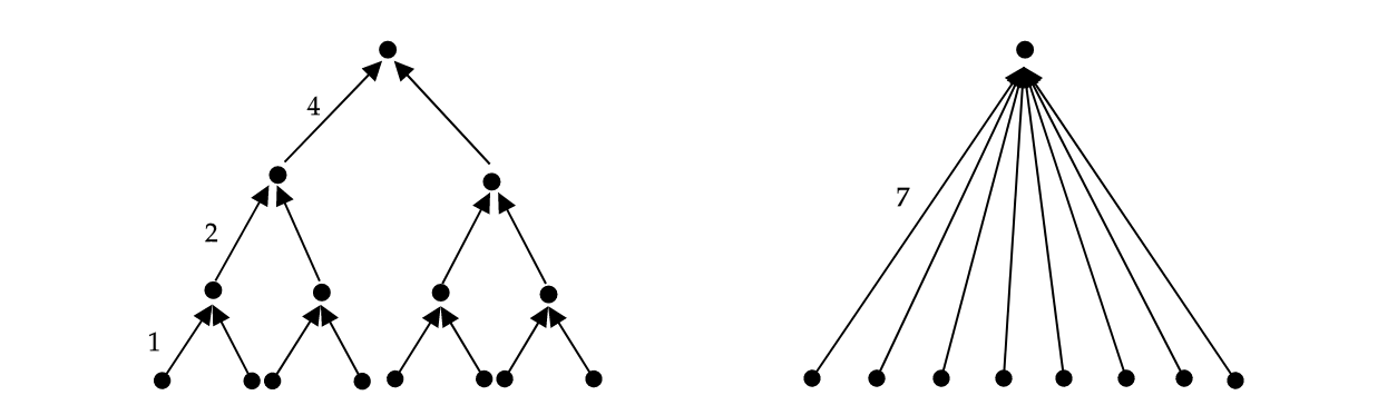
Figure 5: A 2-HST with low inner-constant and subgraph with high inner-constant.

The above shortcoming motivates us to consider metric spaces (for which the doubling dimension is semi-hereditary) and semi-metric spaces (for which the packing dimension is hereditary). We ask whether there exists simple transformations from quasi-metric to metric or semi-metric spaces, and whether these transformations can be used in learning. To this end, define $\rho^{\max}(x,y)=\max\{\rho(x,y),\rho(y,x)\}$ and $\rho^{\min}(x,y)=\min\{\rho(x,y),\rho(y,x)\}$. We can show the following concerning the $\rho^{\max}$ distance function:

Theorem 12

If $(\mathcal{X},\rho)$ is a quasi-metric, then

1. $(\mathcal{X},\rho^{\max})$ is a metric.

2. $\lambda(\mathcal{X},\rho^{\max})$ may be equal to $n$, even if both $\lambda^{\operatorname{out}}(\mathcal{X},\rho)$ and $\lambda^{\operatorname{in}}(\mathcal{X},\rho)$ are constant.

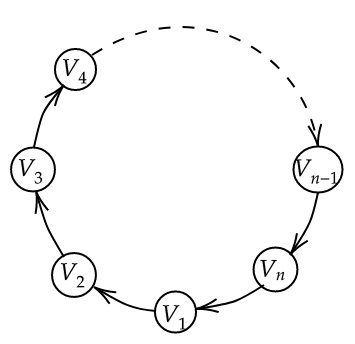
Figure 6: Directed cycle graph

Proof  For the first item: As $\rho$ satisies the triangle inequality, we have $\rho(x,y)\leq\rho(x,z)+\rho(z,y)$ and $\rho(y,x)\leq\rho(y,z)+\rho(z,x)$ for all $x,y,z\in\mathcal{X}$. It follows that

$$\rho^{\max}(x,y) = \max\{\rho(x,y),\rho(y,x)\}$$

$$\leq \max\{\rho(x,z)+\rho(z,y),\rho(y,z)+\rho(z,x)\}$$

$$\leq \max\{\rho(x,z),\rho(z,x)\}+\max\{\rho(y,z),\rho(z,y)\}$$

$$= \rho^{\max}(x,z)+\rho^{\max}(z,y).$$

For the second item: Consider the cycle graph of Figure 6. Clearly, the graph has outer- and inner-constant 2. When we consider the distance function $\rho^{\max}$ operating on this graph, we have that all inter-point distances are in the range $[\frac{n}{2},n-1]$. So a ball of radius $n-1$ rooted an any point covers all points, but a covering of these points by balls of radius $\frac{n-1}{2}$ is of size $n$.  

It follows that quasi-metrics can easily be transformed into metrics, but at the cost of losing the entire structure that permits learning. Even if the original quasi-metric had both low outer- and inner- constants, the resulting metric may have high doubling constant for which no compression and learning guarantees are possible.

Moving to semi-metrics, we can show the following concerning the $\rho^{\min}$ distance function:

Theorem 13

If $(\mathcal{X},\rho)$ is a quasi-metric, then

1. $(\mathcal{X},\rho^{\min})$ is a semi-metric, but may not obey the triangle inequality.

2. $\lambda(\mathcal{X},\rho^{\min})\leq\lambda^{\operatorname{out}}(\mathcal{X},\rho)+\lambda^{\operatorname{in}}(\mathcal{X},\rho)$.

3. $\mu(\mathcal{X},\rho^{\min})\leq(\lambda^{\operatorname{out}}(\mathcal{X},\rho))^{2}+(\lambda^{\operatorname{in}}(\mathcal{X},\rho))^{2}$.

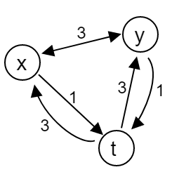
Figure 7: Transformation from quasi-metric to Semi-metric

Proof  For the first item: $\rho^{\min}(x,y)=\min\{\rho(x,y),\rho(y,x)\}\geq 0$, and further $\rho^{\min}(x,y)=\min\{\rho(x,y),\rho(y,x)\}=\min\{\rho(y,x),\rho(x,y)\}=\rho^{\min}(y,x)$, so the distance function is non-negative and symmetric. To show that it may violate the triangle inequality, refer to Figure 7: It is easily verified that the graph satisfies the triangle inequality, however we have $\rho^{\min}(x,y)=3>1+1=\rho^{\min}(x,z)+\rho^{\min}(z,y)$, so the triangle inequality does not hold under $\rho^{\min}$.

For the second item: Take any point $x\in X$ and radius $r$, and let $B$ be the points in $B_{r}(x)$ under distance measure $\rho^{\min}$. Let $B^{\operatorname{in}}\subset B_{r}(X)$ include all points $y\in B_{r}(x)$ satisfying $\rho(y,x)=\rho^{\min}(y,x)$, and let $B^{\operatorname{out}}=B_{r}(X)-B^{\operatorname{in}}$. Now, as $\rho^{\min}$ does not expand distance of $\rho$, the at most $\lambda^{\operatorname{in}}$ points that served as an $\frac{r}{2}$-inner-cover of $B^{\operatorname{in}}$ under $\rho$ still $\frac{r}{2}$-covers those points under $\rho^{\min}$. Likewise, the at most $\lambda^{\operatorname{out}}$ points that served as an $\frac{r}{2}$-outer-cover of $B^{\operatorname{out}}$ under $\rho$ still cover those points under $\rho^{\min}$. The claim follows.

For the third item: The proof is similar to the second item, except we look at the $\frac{r}{4}$-inner-cover and $\frac{r}{4}$-outer-cover points, of which there are (by Lemma 6) at most $(\lambda^{\operatorname{out}}(\mathcal{X},\rho))^{2}$ and $(\lambda^{\operatorname{in}}(\mathcal{X},\rho))^{2}$ respectively. All points covered by a single cover point under $\rho^{\min}$ are within distance $\frac{r}{2}$, and at most one can be a witness for the density constant with respect to an $r$-ball. The claim follows.  

We conclude that if both the inner- and outer-constants are small, we may learn by using the $\rho^{\min}$ operator to transform the quasi-metric into a semi-metric. The semi-metric has the useful property that its learning is controlled by the density constant, which is a hereditary property. Nevertheless, this transformation comes at a price, as the margin (which controls learning together with the density constant) is now reduced to $\min\{\rho^{\pm},\rho^{\mp}\}$ (where $\rho^{\pm}=\rho(S_{+},S_{-})$ and $\rho^{\mp}=\rho(S_{-},S_{+})$). In contrast, the quasi-metric bounds of Theorem 7 allow us to choose whichever value of $\rho^{\pm}$ and $\rho^{\mp}$ yields better bounds.

References

- Anari and Gharan (2015) Nima Anari and Shayan Oveis Gharan. Effective-resistance-reducing flows, spectrally thin trees, and asymmetric tsp. In 2015 IEEE 56th Annual Symposium on Foundations of Computer Science, pages 20–39, 2015.
- Asadpour et al. (2010) Arash Asadpour, Michel X Goemans, Aleksander Madry, Shayan Oveis Gharan, and Amin Saberi. An -approximation algorithm for the asymmetric traveling salesman problem. In Proceedings of the twenty-first annual ACM-SIAM symposium on Discrete Algorithms, pages 379–389, 2010.
- Assouad (1983) P. Assouad. Plongements lipschitziens dans . Bull. Soc. Math. France, 111(4):429–448, 1983.
- Bartal (1996) Yair Bartal. Probabilistic approximation of metric spaces and its algorithmic applications. In In 37th Annual Symposium on Foundations of Computer Science, pages 184–193, 1996.
- Chen et al. (2006) S. Chen, W. Li, S. Tian, and Z. Mao. On optimization problems in quasi-metric spaces. In 2006 International Conference on Machine Learning and Cybernetics, pages 865–870, 2006.
- (6) R. Cole and L. Gottlieb. Searching dynamic point sets in spaces with bounded doubling dimension. In STOC ’06, pages 574–583.
- Doitchinov (1988) Doitchin Doitchinov. On completeness in quasi-metric spaces. Topology and its Applications, 30(2):127 – 148, 1988.
- Dung et al. (2019) Nguyen Dung, An Tran Van, and Hang Hang. Remarks on frink’s metrization technique and applications. Fixed Point Theory, 20:157–176, 03 2019.
- Frieze et al. (1982) Alan M Frieze, Giulia Galbiati, and Francesco Maffioli. On the worst-case performance of some algorithms for the asymmetric traveling salesman problem. Networks, 12(1):23–39, 1982.
- Frink (1937) Aline H Frink. Distance functions and the metrization problem. Bulletin of the American Mathematical Society, 43(2):133–142, 1937.
- Gottlieb and Krauthgamer (2013) Lee-Ad Gottlieb and Robert Krauthgamer. Proximity algorithms for nearly doubling spaces. SIAM Journal on Discrete Mathematics, 27(4):1759–1769, 2013.
- Gottlieb et al. (2014a) Lee-Ad Gottlieb, Aryeh Kontorovich, and Robert Krauthgamer. Efficient classification for metric data. IEEE Transactions on Information Theory, 60(9):5750–5759, 2014a.
- Gottlieb et al. (2014b) Lee-Ad Gottlieb, Aryeh Kontorovich, and Pinhas Nisnevitch. Near-optimal sample compression for nearest neighbors. In Advances in Neural Information Processing Systems, pages 370–378, 2014b.
- Gottlieb et al. (2017) Lee-Ad Gottlieb, Aryeh Kontorovich, and Pinhas Nisnevitch. Nearly optimal classification for semimetrics. The Journal of Machine Learning Research, 18(1):1233–1254, 2017.
- Goubault-Larrecq (2017) Jean Goubault-Larrecq. Complete quasi-metrics for hyperspaces, continuous valuations, and previsions. arXiv preprint arXiv:1707.03784, 2017.
- Graepel et al. (2005) Thore Graepel, Ralf Herbrich, and John Shawe-Taylor. Pac-bayesian compression bounds on the prediction error of learning algorithms for classification. Machine Learning, 59(1-2):55–76, 2005.
- Gupta et al. (2003) Anupam Gupta, Robert Krauthgamer, and James R. Lee. Bounded geometries, fractals, and low-distortion embeddings. In FOCS, pages 534–543, 2003.
- Gutiérrez-Naranjo et al. (2002) Miguel A. Gutiérrez-Naranjo, José A. Alonso-Jiménez, and Joaquín Borrego-Díaz. A quasi-metric for machine learning. In Advances in Artificial Intelligence — IBERAMIA 2002, pages 193–203, 2002.
- Har-Peled and Mendel (2006) S. Har-Peled and M. Mendel. Fast construction of nets in low-dimensional metrics and their applications. SIAM Journal on Computing, 35(5):1148–1184, 2006.
- Klimo et al. (2018) M. Klimo, O. Škvarek, P. Tarábek, O. Šuch, and J. Hrabovsky. Nearest neighbor classification in minkowski quasi-metric space. In 2018 World Symposium on Digital Intelligence for Systems and Machines (DISA), pages 227–232, 2018.
- Kontorovich and Weiss (2014) Aryeh Kontorovich and Roi Weiss. Maximum margin multiclass nearest neighbors. In ICML, pages 892–900, 2014.
- (22) R. Krauthgamer and J.R. Lee. Navigating nets: Simple algorithms for proximity search. In SODA ’04, pages 791–801.
- Künzi (2001) Hans-Peter A Künzi. Nonsymmetric distances and their associated topologies: about the origins of basic ideas in the area of asymmetric topology. In Handbook of the history of general topology, pages 853–968. Springer, 2001.
- Lawvere (1973) F. William Lawvere. Metric spaces, generalized logic, and closed categories. Rendiconti del Seminario Matematico e Fisico di Milano, 43(1):135–166, 1973.
- Luxburg and Bousquet (2004) Ulrike von Luxburg and Olivier Bousquet. Distance-based classification with lipschitz functions. Journal of Machine Learning Research, 5(Jun):669–695, 2004.
- Mémoli et al. (2018) Facundo Mémoli, Anastasios Sidiropoulos, and Vijay Sridhar. Quasimetric embeddings and their applications. Algorithmica, 80(12):3803–3824, 2018.
- Reilly (1976) Ivan L. Reilly. A note on quasi metric spaces. Proc. Japan Acad., 52(8):428–430, 1976.
- Schroeder (2006) Viktor Schroeder. Quasi-metric and metric spaces. Conformal Geometry and Dynamics of the American Mathematical Society, 10(18):355–360, 2006.
- Shalev-Shwartz and Ben-David (2014) Shai Shalev-Shwartz and Shai Ben-David. Understanding machine learning: From theory to algorithms. Cambridge university press, 2014.
- Shao-Bai Chen et al. (2005) Shao-Bai Chen, Sen-Ping Tian, and Zong-Yuan Mao. Quasi-pseudo-metric of measurable classifiers. In 2005 International Conference on Machine Learning and Cybernetics, volume 7, pages 4340–4344 Vol. 7, 2005.
- Stojmirovic (2008) Aleksandar Stojmirovic. Quasi-metrics, similarities and searches: aspects of geometry of protein datasets. arXiv preprint arXiv:0810.5407, 2008.
- Stoltenberg (1969) Ronald A. Stoltenberg. On quasi-metric spaces. Duke Math. J., 36(1):65–71, 03 1969.
- Svensson et al. (2017) Ola Svensson, Jakub Tarnawski, and László A Végh. A constant-factor approximation algorithm for the asymmetric traveling salesman problem. arXiv preprint arXiv:1708.04215, 2017.
- Wilson (1936) W. Wilson. On quasi-metric spaces. American Journal of Mathematics, 53(3):675–684, 1936.
- Zhang et al. (2019) T. Zhang, Y. Gao, L. Chen, G. Chen, and S. Pu. Efficient similarity search on quasi-metric graphs. IEEE Access, 7:101496–101512, 2019.