On the group of spheromorphisms of
the homogeneous non-locally finite tree


Yury A. Neretin111The research was supported by the grants FWF, Projects P28421, P31591.

Consider a tree $\mathbb{T}$, all whose vertices have countable valence; its boundary is the Baire space $\mathbb{B}\simeq{\mathbb{N}}^{\mathbb{N}}$; continued fractions expansions identify the set of irrational numbers ${\mathbb{R}}\setminus{\mathbb{Q}}$ with $\mathbb{B}$. Removing $k$ edges from $\mathbb{T}$ we get a forest consisting of copies of $\mathbb{T}$. A spheromorphism (or hierarchomorphism) of $\mathbb{T}$ is an isomorphisms of two such subforests considered as a transformation of $\mathbb{T}$ or of $\mathbb{B}$. Denote the group of all spheromorphisms by $\mathop{\mathrm{Hier}}\nolimits(\mathbb{T})$. We a show that the correspondence ${\mathbb{R}}\setminus{\mathbb{Q}}\simeq\mathbb{B}$ sends the Thompson group realized by piecewise $\mathop{\mathrm{PSL}}\nolimits_{2}({\mathbb{Z}})$-transformations to a subgroup of $\mathop{\mathrm{Hier}}\nolimits(\mathbb{T})$. We construct some unitary representations of the group $\mathop{\mathrm{Hier}}\nolimits(\mathbb{T})$, show that the group of automorphisms $\mathop{\mathrm{Aut}}\nolimits(\mathbb{T})$ is spherical in $\mathop{\mathrm{Hier}}\nolimits(\mathbb{T})$, and describe the train (enveloping category) of $\mathop{\mathrm{Hier}}\nolimits(\mathbb{T})$.

1 Introduction

1.1. The tree $\mathbb{T}$ and its boundary $\partial\mathbb{T}$. For a set $A$ denote by $\#A$ the number of its elements. Denote by ${\mathbb{Z}}_{+}$ the set of all nonnegative integers.

Recall that a tree $T$ is a connected graph without cycles. Denote by $\mathop{\mathrm{vert}}\nolimits(T)$ the set of its vertices, $\mathop{\mathrm{edge}}\nolimits(T)$ the set of its edges. A forest is a disjoint union of trees. We admit both finite and infinite trees.

Denote by $\mathbb{T}$ the tree such that each vertex is contained in a countable number of edges. Such a tree is unique up to isomorphisms of trees. It can be realized in the following form. Vertices of $\mathbb{T}$ are enumerated by finite collections

(s1,s2,…,sm),whereΒ s1βˆˆβ„€+,Β s2, …,Β smβˆˆβ„•,subscript𝑠1subscript𝑠2…subscriptπ‘ π‘šwhereΒ s1βˆˆβ„€+,Β s2, …,Β smβˆˆβ„•,(s_{1},s_{2},\dots,s_{m}),\qquad\text{where $s_{1}\in{\mathbb{Z}}_{+}$, $s_{2}$, \ldots, $s_{m}\in{\mathbb{N}}$,} (1.1)

where $m=0$, 1, 2, …. We admit an empty collection, below we call such vertex the initial point222We do not use the term ’root’ since we regard $\mathbb{T}$ as a non-rooted tree. of $\mathbb{T}$ and denote by ’$\boldsymbol{\cdot}$’. Edges have form

(s1,…,sm)​—​(s1,…,sm,sm+1).subscript𝑠1…subscriptπ‘ π‘šβ€”subscript𝑠1…subscriptπ‘ π‘šsubscriptπ‘ π‘š1(s_{1},\dots,s_{m})\,\text{---}\,(s_{1},\dots,s_{m},s_{m+1}).

We say that a way in $\mathbb{T}$ is a sequence of pairwise distinct vertices $a_{0}$, $a_{1}$, $a_{2}$, …such that $a_{j}$ and $a_{j+1}$ are connected by an edge. We say that two ways $a=\{a_{0},a_{1},a_{2},\dots\}$, $b=\{b_{0},b_{1},b_{2},\dots\}$ are equivalent if there is $k\in{\mathbb{Z}}$ such that for sufficiently large $j$ we have $b_{j}=a_{j+k}$. The boundary $\partial\mathbb{T}$ of $\mathbb{T}$ is the set of all ways defined up to this equivalence. Fix a vertex $r$. Then for any point $\omega\in\partial\mathbb{T}$ there is a unique way starting at $r$ and coming to $\omega$ (formally, the last phrase means that there is a unique representative of $\omega$ starting at $r$). Define a distance between ways $a=\{r,a_{1},a_{2},\dots\}$ $b=\{r,b_{1},b_{2},\dots\}$ by $\mathrm{dist}_{r}(a,b)=2^{-j}$, where $j$ is the first number such that ajβ‰ bjsubscriptπ‘Žπ‘—subscript𝑏𝑗a_{j}\neq b_{j}. Then $\partial\mathbb{T}$ becomes a complete totally disconnected metric space. Distances $\mathrm{dist}_{r}(\cdot,\cdot)$ depend on $r$ but they define the same topology.

Choosing $r=\boldsymbol{\cdot}$, we identify $\partial\mathbb{T}$ with the set of all sequences

(s1,s2,s3​…),whereΒ s1βˆˆβ„€+,Β s2,Β s3,β‹―βˆˆβ„•,subscript𝑠1subscript𝑠2subscript𝑠3…whereΒ s1βˆˆβ„€+,Β s2,Β s3,β‹―βˆˆβ„•,(s_{1},s_{2},s_{3}\dots),\qquad\text{where $s_{1}\in{\mathbb{Z}}_{+}$, $s_{2}$, $s_{3},\dots\in{\mathbb{N}}$,}

1.2. The Baire space and continued fractions. Recall (see, e.Β g., [8]) that the Baire space $\mathbb{B}$ is the topological space homeomorphic to the countable product of countable discrete spaces,

$$\mathbb{B}\simeq{\mathbb{N}}^{\mathbb{N}}={\mathbb{N}}\times{\mathbb{N}}\times{\mathbb{N}}\times\dots$$

equipped with the Tikhonov topology. Clearly, the boundary $\partial\mathbb{T}$ is $\mathbb{B}$.

The Baire space can be identified with the set ${\mathbb{R}}\setminus{\mathbb{Q}}$ of irrational numbers. Namely, let $x\in{\mathbb{R}}\setminus{\mathbb{Q}}$. Consider its continued fraction decomposition,

$$x=u_{0}+\cfrac{1}{u_{1}+\cfrac{1}{u_{2}+\cfrac{1}{u_{3}+\cfrac{1}{u_{4}+\dots}}}}=:[u_{0};u_{1},u_{2},u_{3},\dots].$$

For irrational $x$ the continued fraction is infinite, therefore we have an identification

$${\mathbb{R}}\setminus{\mathbb{Q}}\simeq{\mathbb{Z}}\times{\mathbb{N}}\times{\mathbb{N}}\times{\mathbb{N}}\times\dots\simeq\mathbb{B}$$

The Baire space $\mathbb{B}$ and this correspondence had a fundamental role in works of Luzin on descriptive set theory in 1920s, see [11], [12].

1.3. The group of spheromorphisms. Denote by $\mathop{\mathrm{Aut}}\nolimits(\mathbb{T})$ the group of all automorphisms of $\mathbb{T}$. We define the topology on $\mathop{\mathrm{Aut}}\nolimits(\mathbb{T})$ assuming that all point-wise stabilizers $\mathcal{K}(J)$ of finite subtrees $J\subset\mathbb{T}$ are open subgroups in $\mathop{\mathrm{Aut}}\nolimits(\mathbb{T})$. We get a Polish group333i.Β e., a topological group that is homeomorphic (as a topological space) to a complete metric space, see, e.g.? [8]..

Consider a proper subtree $S\subset\mathbb{T}$ isomorphic to $\mathbb{T}$. We say that $S$ is a $(\mathbb{T})$-subtree if there is only finite number of edges $[a,b]$ of $\mathbb{T}$ such that $a\in S$ and $b\notin S$, see Fig. 1.a. An intersection of two $(\mathbb{T})$-subtrees is $(\mathbb{T})$-subtree or the empty set. If $(\mathbb{T})$-subtrees $P$, $Q$ have a common vertex, then $P\cup Q$ is a $(\mathbb{T})$-subtree.

a)Refer to caption\mathrm{a)}\qquad\epsfbox{inftree.1}
b)Refer to caption\mathrm{b)}\epsfbox{inftree.2}
Figure 1: Refs. to Subsect. 1 and 2.
a) A $(\mathbb{T})$-subtree.
b) The corresponding frame.

We say that a $(\mathbb{T})$-covering forest of $\mathbb{T}$ is a finite collection of disjoint $(\mathbb{T})$-subtrees $S_{1}$, …, $S_{k}$ such that

$$\mathop{\mathrm{vert}}\nolimits(\mathbb{T})=\bigcup\mathop{\mathrm{vert}}\nolimits(S_{j}),\qquad\text{the set $\mathop{\mathrm{edge}}\nolimits(\mathbb{T})\setminus\bigcup\mathop{\mathrm{edge}}\nolimits(S_{j})$ is finite.}$$

In other words, a $(\mathbb{T})$-covering forest is obtained from $\mathbb{T}$ by a removing a finite collection of edges.

Let $S_{1}$, …, $S_{k}$ and $R_{1}$, …, $R_{k}$ be two $(\mathbb{T})$-covering forests. A spheromorphism (or hierarchomorphism) $g$ of $\mathbb{T}$ is a collection $\{g^{(j)}\}$ of isomorphisms $g^{(j)}:S_{j}\to R_{j}$. Notice that a spheromorphism $g$ determines a permutation

$$\mathop{\mathrm{vert}}\nolimits(\mathbb{T})\to\mathop{\mathrm{vert}}\nolimits(\mathbb{T})$$ (1.2)

and a homeomorphism

$$\partial\mathbb{T}\to\partial\mathbb{T}.$$ (1.3)

These maps determine one another, two spheromorphisms are equal if the coresponding maps (1.2) (or, equivalently, (1.3)) coincide, we denote them by the same symbol $g$.

Let $\{g^{(j)}\}:\{S^{(j)}\}\to\{R^{(j)}\}$, $\{h^{(l)}\}:\{Q^{(l)}\}\to\{T^{(l)}\}$ be spheromorphisms. Their product is the collection of isomorphisms of $(\mathbb{T})$-subtrees.

$$\{h^{(l)}g^{(j)}\}:\{(g^{(j)})^{-1}(R^{(j)}\cap Q^{(l)})\}\to\{h^{(l)}(R^{(j)}\cap Q^{(l)})\}.$$

Denote by $\mathop{\mathrm{Hier}}\nolimits(\mathbb{T})$ the group of all spheromorphisms. By definition, the group $\mathop{\mathrm{Hier}}\nolimits(\mathbb{T})$ is embedded to the group of all permutations of $\mathop{\mathrm{vert}}\nolimits(\mathbb{T})$ and the group of all homeomorphisms of $\partial\mathbb{T}$.

We define a topology on $\mathop{\mathrm{Hier}}\nolimits(\mathbb{T})$ from two conditions:

a) the induced topology on $\mathop{\mathrm{Aut}}\nolimits(\mathbb{T})\subset\mathop{\mathrm{Hier}}\nolimits(\mathbb{T})$ coincides with the natural topology on $\mathop{\mathrm{Aut}}\nolimits(\mathbb{T})$.

b) The topology on the countable homogeneous space $\mathop{\mathrm{Hier}}\nolimits(\mathbb{T})/\mathop{\mathrm{Aut}}\nolimits(\mathbb{T})$ is discrete.

In this way we get a structure of a Polish group on $\mathop{\mathrm{Hier}}\nolimits(\mathbb{T})$.

1.4. Thompson group and the group of spheromorphisms. Consider the natural action of the group $\mathop{\mathrm{PGL}}\nolimits_{2}({\mathbb{Z}})$ on the real projective line ${\mathbb{R}}\mathbb{P}^{1}$ by linear fractional transformations,

x↦a​x+bc​x+d,whereΒ a,Β b,Β c,Β dβˆˆβ„€,Β a​dβˆ’b​c=Β±1.maps-toπ‘₯π‘Žπ‘₯𝑏𝑐π‘₯𝑑whereΒ a,Β b,Β c,Β dβˆˆβ„€,Β adβˆ’bc=Β±1.x\mapsto\frac{ax+b}{cx+d},\qquad\text{where $a$, $b$, $c$, $d\in{\mathbb{Z}}$, $ad-bc=\pm 1$.}

It contains a subgroup $\mathop{\mathrm{PSL}}\nolimits_{2}({\mathbb{Z}})$ consisting of transformations with $ad-bc=1$. Clearly, the set ${\mathbb{Q}}$ of rational numbers is invariant with respect to such transformations, therefore $\mathop{\mathrm{PGL}}\nolimits_{2}({\mathbb{Z}})$ acts also on the set of irrational numbers ${\mathbb{R}}\setminus{\mathbb{Q}}$. Next, consider the Thompson group $\mathrm{T\!h}$ of all continuous piece-wise $\mathop{\mathrm{PSL}}\nolimits_{2}({\mathbb{Z}})$-transformations. It is easy to show that such transformations have smoothness $C^{1}$ and points of break of the second derivative are rational.

More constructive description of such transformations
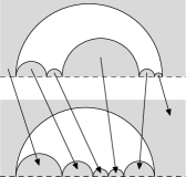
 is given on Fig. 2.

Refer to caption

,   Refer to caption

Figure 2: 3 Refs. to Subsect. 1.
a) Consider the Lobachevsky plane $\Lambda:\mathop{\mathrm{Im}}\nolimits z>0$. Lines on $\Lambda$ are semicircles and rays orthogonal to the line $\mathop{\mathrm{Im}}\nolimits z=0$. Consider the line $\mathop{\mathrm{Re}}\nolimits z=0$ and all its images under elements of the group $\mathop{\mathrm{PSL}}\nolimits_{2}({\mathbb{Z}})$. We get a family $\mathcal{Z}$ of lines, each line separates $\Lambda$ into two half-planes (on the Figure they are half-disks, complements to half-disks, or right angles). For any pair of two such half-planes there is a unique element of $\mathop{\mathrm{PSL}}\nolimits_{2}({\mathbb{Z}})$ sending one half-plane to another.
b) We take two ideal $n$-gons $U$, $V$, whose sides are contained in the family $\mathcal{Z}$. Let $A_{1}$, …, $A_{n}$ be complementary half-planes to $U$ and $B_{1}$, …, $B_{n}$ to $V$ (enumerated in according to the natural cyclic order). Consider a cyclic permutation $j\mapsto k+j(\mod n)$ of the set $\{1,2,\dots,n\}$. For each $j$ consider the canonical $\mathop{\mathrm{PSL}}\nolimits(2,{\mathbb{Z}})$-transformation $A_{j}\mapsto B_{j+k}$. In this way we get a piece-wise $\mathop{\mathrm{PSL}}\nolimits_{2}({\mathbb{Z}})$-transformation of ${\mathbb{R}}\mathbb{P}^{1}$.

Remark. The Thompson group $\mathrm{T\!h}$ was defined by Richard Thompson in 1966 as a counterexample, later it became clear that it is a very interesting discrete group with unusual properties, see, e.Β g., [4], [6], [3]. May be the most strange is its relation with the Minkowski function $?(x)$ (apparently observed by Sergiescu, see [3]). $\boxtimes$

The group $\mathrm{T\!h}$ acts on ${\mathbb{R}}\setminus{\mathbb{Q}}$ and therefore acts on the Baire space $\partial\mathbb{T}$. Theorem 3.2 shows that the Thompson group acts on $\partial\mathbb{T}$ by spheromorphisms444Let $[a_{0};a_{1},a_{2},\dots]$ be a continued fraction, $[b_{0};b_{1},b_{2},\dots]$ be its image under $\mathop{\mathrm{PSL}}\nolimits_{2}({\mathbb{Z}})$-transformation. Clearly, there is $m\in{\mathbb{Z}}$ such that for sufficiently large $j$ we have $b_{j+m}=a_{j}$. Therefore the same holds for transformations from the Thompson group. Notice that such tail equivalence does not imply our statement..

1.5. The train of $\mathop{\mathrm{Hier}}\nolimits(\mathbb{T})$. In Section 4 we get a train construction in the sense of [16]. Recall that quite often a pair $G\supset K$ of infinite-dimensional groups generates a natural category (train of $(G,K)$) acting in unitary representations of $G$, such groups are called $(G,K)$-pairs. In our case $G=\mathop{\mathrm{Hier}}\nolimits(\mathbb{T})$, $K$ is the stabilizer $\mathcal{K}\subset\mathop{\mathrm{Aut}}\nolimits(\mathbb{T})$ of a vertex.

Namely, let $J$ be a nonempty555The construction below does not hold for double cosets $\mathop{\mathrm{Aut}}\nolimits(\mathbb{T})\setminus\mathop{\mathrm{Hier}}\nolimits(\mathbb{T})/\mathop{\mathrm{Aut}}\nolimits(\mathbb{T})$. finite subtree in $\mathbb{T}$, let $\mathcal{K}(J)\subset\mathop{\mathrm{Aut}}\nolimits(\mathbb{T})$ be its point-wise stabilizer. In Subsect. 4 we give a combinatorial description of double coset spaces666Let $G$ be a group, $K_{1}$, $K_{2}$ subgroups. A double coset is a subset in $G$ of the form $K_{1}gK_{2}$, where $g\in G$. The set $K_{1}\setminus G/K_{2}$ denotes the space of all double cosets.
If a subgroup $K$ is compact, then there is a natural structure of a ’hypergroup’ on $K\setminus G/K$, i.Β e., we have a map from $K\setminus G/K\times K\setminus G/K$ to the space $\mathcal{M}(K\setminus G/K)$ of measures on $K\setminus G/K$. Namely, we consider uniform probabilistic measures $\mu_{g_{1}}$, $\mu_{g_{2}}$ on double cosets $Kg_{1}K$, $Kg_{2}K$, decompose their convolution $\mu_{g_{1}}*\mu_{g_{2}}=\int_{K\setminus G/K}\mu_{g}\,d\nu(g)$, and get a probabilistic measure $\nu$ on $K\setminus G/K$ depending on $Kg_{1}K$, $Kg_{2}K$.
The situation discussed below has not analogs for locally compact groups and is relatively usual for infinite dimensional groups, namely we have associative multiplications on sets Kβˆ–G/K𝐾𝐺𝐾K\setminus G/K, where G=Hier(𝕋)𝐺Hier𝕋G=\mathop{\mathrm{Hier}}\nolimits(\mathbb{T}), K=𝒦​(J)𝐾𝒦𝐽K=\mathcal{K}(J).
𝒦​(J1)βˆ–Hier(𝕋)/𝒦​(J2)𝒦subscript𝐽1Hier𝕋𝒦subscript𝐽2\mathcal{K}(J_{1})\setminus\mathop{\mathrm{Hier}}\nolimits(\mathbb{T})/\mathcal{K}(J_{2}) in terms of colored graphs. Next, we show that there is a natural βŠ™direct-product\odot-multiplication

$$\mathcal{K}(J_{1})\setminus\mathop{\mathrm{Hier}}\nolimits(\mathbb{T})/\mathcal{K}(J_{2})\,\,\times\mathcal{K}(J_{2})\setminus\mathop{\mathrm{Hier}}\nolimits(\mathbb{T})/\mathcal{K}(J_{3})\,\,\longrightarrow\,\,\mathcal{K}(J_{1})\setminus\mathop{\mathrm{Hier}}\nolimits(\mathbb{T})/\mathcal{K}(J_{3}),$$

and it determines a structure of a category. Objects of the category $\mathfrak{Hi}$ are nonempty finite subtrees $J\subset\mathbb{T}$, morphisms are double cosets,

$$\mathop{\mathrm{Mor}}\nolimits_{\mathfrak{Hi}}(J,I):=\mathcal{K}(I)\setminus\mathop{\mathrm{Hier}}\nolimits(\mathbb{T})/\mathcal{K}(J).$$

Consider a unitary representation $\rho$ of the group $\mathop{\mathrm{Hier}}\nolimits(\mathbb{T})$ in a Hilbert space $V$. Denote by $V(J)\subset V$ the subspace of all $\mathcal{K}(J)$-fixed vectors in $V$. Denote by $P(J)$ the operator of orthogonal projection to $V(J)$. For any subtrees $I$, $J$ and $g\in\mathop{\mathrm{Hier}}\nolimits(\mathbb{T})$ we define operators

$$\widetilde{\rho}_{I,J}(g)=P(I)\,\rho(g)\,P(J):\,V(J)\to V(I).$$

This operator depends only on the double coset $\mathfrak{g}=\mathcal{K}(I)\,g\,\mathcal{K}(J)$ containing $g$.

We show (Theorem 4.10) that for $\mathfrak{g}_{1}\in\mathop{\mathrm{Mor}}\nolimits(J_{2},J_{1})$, $\mathfrak{g}_{2}\in\mathop{\mathrm{Mor}}\nolimits(J_{3},J_{2})$ we have

$$\widetilde{\rho}_{J_{1},J_{2}}(\mathfrak{g}_{1})\,\widetilde{\rho}_{J_{2},J_{3}}(\mathfrak{g}_{2})=\widetilde{\rho}_{J_{1},J_{3}}(\mathfrak{g}_{1}\odot\mathfrak{g}_{2}).$$

Notice, that this operation is a representative of a huge zoo of train constructions for $(G,K)$-pairs (see, e. g., [23], [22], [16], [18]).

1.6. Unitary representations of $\mathop{\mathrm{Hier}}\nolimits(\mathbb{T})$. We show that $\mathop{\mathrm{Hier}}\nolimits(\mathbb{T})\supset\mathop{\mathrm{Aut}}\nolimits(\mathbb{T})$ is a spherical pair, i.e., any irreducible unitary representation of $\mathop{\mathrm{Hier}}\nolimits(\mathbb{T})$ has at most one (up to a scalar factor) non-zero $\mathop{\mathrm{Aut}}\nolimits(\mathbb{T})$-fixed vector (Theorem 5.1).

We also show that $\mathop{\mathrm{Hier}}\nolimits(\mathbb{T})$ has non-trivial $\mathop{\mathrm{Aut}}\nolimits(\mathbb{T})$-spherical representations. In fact, we construct embeddings of $\mathop{\mathrm{Hier}}\nolimits(\mathbb{T})$ to two Olshanski’s spherical $(G,K)$-pairs, the first one is related to infinite-symmetric groups (Subsect. 2), the second is related to classical groups (Sect.6). In both cases the subgroup $\mathop{\mathrm{Aut}}\nolimits(\mathbb{T})$ embeds to $K$, restricting $K$-spherical representations777In the both cases classification of $K$-spherical representations of $G$ is known, see [23], [24]. of $G$ to $\mathop{\mathrm{Hier}}\nolimits(\mathbb{T})$ we get $\mathop{\mathrm{Aut}}\nolimits(\mathbb{T})$-spherical representations of $\mathop{\mathrm{Hier}}\nolimits(\mathbb{T})$.

1.7. Similar groups. Consider the Bruhat–Tits tree $\mathcal{T}_{p}$, i.Β e., the tree whose vertices have valence $p+1$. According Bruhat and Tits, such trees are $p$-adic couneterparts of the Lobachevsky plane, and more generally of noncompact rank 1 Riemannian symmetric spaces, see e.g., [17], Sect. 10.4. Applying the same approach to a non-Archimedean field with discrete absolute value and countable residue field888For instance, we can consider the field of formal Laurent series over ${\mathbb{Q}}$, then the group $\mathop{\mathrm{PGL}}\nolimits_{2}$ over this field acts in a natural way by automorphisms of the tree $\mathbb{T}$., we get the tree $\mathbb{T}$. The group $\mathop{\mathrm{Aut}}\nolimits(\mathcal{T}_{p})$ of all automorphisms of $\mathcal{T}_{p}$ is counterpart of real and $p$-adic groups $\mathop{\mathrm{SL}}\nolimits_{2}$ on the level of representation theory, see [20]. A spheromorphism of $\mathcal{T}_{p}$ is a homeomorphism $q$ of the boundary $\partial\mathcal{T}_{p}$ such that for any point of the boundary there is a neighborhood, where $q$ coincides with an automorphism of the tree. The group $\mathop{\mathrm{Hier}}\nolimits(\mathcal{T}_{p})$ of all spheromorphisms was defined in [13]–[14] as a counterpart of the group $\mathop{\mathrm{Diff}}\nolimits(S^{1})$ of diffeomorphisms of the circle and the group999In particular, there is a natural inclusion $\mathop{\mathrm{Diff}}\nolimits(\mathbb{P}{\mathbb{Q}}_{p}^{1})\subset\mathop{\mathrm{Hier}}\nolimits(\mathcal{T}_{p})$. $\mathop{\mathrm{Diff}}\nolimits(\mathbb{P}{\mathbb{Q}}_{p}^{1})$ of locally analytic diffeomorphisms of the $p$-adic projective line $\mathbb{P}{\mathbb{Q}}_{p}^{1}$. The group $\mathop{\mathrm{Hier}}\nolimits(\mathcal{T}_{p})$ has numerous properties unusual for locally compact groups, see a long list of references in [19].

So we have a family of groups including

$\mathop{\mathrm{Diff}}\nolimits(S^{1})$, $\mathop{\mathrm{Diff}}\nolimits(\mathbb{P}{\mathbb{Q}}_{p}^{1})$, $\mathop{\mathrm{Hier}}\nolimits(\mathcal{T}_{p})$, $\mathop{\mathrm{Hier}}\nolimits(\mathbb{T})$. (1.4)

The group $\mathop{\mathrm{Hier}}\nolimits(\mathbb{T})$ looks like a monster, however as an object of representation theory it is simpler than its relatives. The reason is a presence of the subgroup $\mathcal{K}(\boldsymbol{\cdot})$, which is ’heavy’ in the sense of [16]. So understanding of the group $\mathop{\mathrm{Hier}}\nolimits(\mathbb{T})$ can be useful as a standpoint for investigation of other groups (1.4).

Acknowledgments. The author is grateful to Vlad Sergiescu and Nikita Gorbatyuk for discussions of this topic.

2 Preliminary remarks

2.1. Frames of $(\mathbb{T})$-subtrees. For a $(\mathbb{T})$-subtree $S$ we mark all edges connecting $S$ with $\mathbb{T}\setminus S$. Call the frame of $S$ the minimal subtree in $\mathbb{T}$ containing marked edges.

Notice that terminal edges of the frame are precisely marked edges. If a frame has more than two vertices then it uniquely determines a $(\mathbb{T})$-tree. We remove its terminal edges of a frame from $\mathbb{T}$, then $\mathbb{T}$ splits into a disjoint union of $(\mathbb{T})$-trees, we choose a piece that contains non-terminal vertices of the frame101010If the frame has only two vertices, then $(\mathbb{T})$ splits into two parts, and we can not distinguish them..

Clearly, any finite subtree with $\geqslant 2$ vertices can be a frame and the isomorphism class of a frame is a unique invariant of $(\mathbb{T})$-subtrees under the action of $\mathop{\mathrm{Aut}}\nolimits(\mathbb{T})$.

Remark. In [15] there was defined a smaller group of spheromorphisms $\mathop{\mathrm{Hier}}\nolimits^{\circ}(\mathbb{T})\subset\mathop{\mathrm{Hier}}\nolimits(\mathbb{T})$. Namely, we consider a $(\mathbb{T})$-covering forest $\{S_{1},\dots,S_{k}\}$ and a collection $g_{j}\in\mathop{\mathrm{Aut}}\nolimits(\mathbb{T})$ such that $g_{j}S_{j}$ is a $(\mathbb{T})$-covering forest. Then we have a spheromorphism in the sense of the previous definition. However, our definition allows isomorphisms $S_{j}\to R_{j}$, which have not extensions to automorphisms of the whole tree $\mathbb{T}$. $\boxtimes$

2.2. The perfect compatible $(\mathbb{T})$-forest for a spheromorphism. We say that a $(\mathbb{T})$-subtree $S$ is compatible with a spheromorphism $g$ if the map $g:\mathop{\mathrm{vert}}\nolimits(S)\to\mathop{\mathrm{vert}}\nolimits(\mathbb{T})$ is an embedding of trees. We say that a $(\mathbb{T})$-covering forest $\{S_{j}\}$ is compatible with $g$ if all trees $S_{j}$ are compatible with $g$.

Lemma 2.1

For any spheromorphism $g$ there is a unique compatible $(\mathbb{T})$-covering forest $P_{1}$, …, $P_{l}$ such that any compatible $(\mathbb{T})$-covering forest is obtained by removing a finite collection of edges from the forest $\{P_{i}\}$.

Let us call such forest the perfect $(\mathbb{T})$-covering forest for $g$.

Proof. Consider a compatible $(\mathbb{T})$-covering forest $\{S_{j}\}$ with minimal possible number of trees, say $l$. Let $\{Q_{\alpha}\}$ be another covering. Let some $Q_{\beta}$ be not contained in any $S_{i}$. Consider trees $S_{\gamma_{1}}$, $S_{\gamma_{2}}$, …, $S_{\gamma_{m}}$ that have nonempty intersections with $Q_{\beta}$, by definition $m\geqslant 2$. Then

$$\widetilde{S}:=Q_{\beta}\cup\bigl{(}\cup S_{\gamma_{i}}\bigr{)}=\cup S_{\gamma_{i}}$$

is a $(\mathbb{T})$-subtree compatible with $g$. We get a compatible $(\mathbb{T})$-covering forest with $l-m+1<l$ elements. $\square$

2.3. Skeletons of $(\mathbb{T})$-covering forests. Consider a $(\mathbb{T})$-covering forest $\{S_{j}\}$. Paint blue all edges that do not contained in the trees $S_{j}$. Consider the minimal subtree $\Sigma\subset\mathbb{T}$ containing all blue edges, paint remaining edges black. We call the colored tree obtained in this way the skeleton $\mathop{\mathrm{Skel}}\nolimits\{S_{j}\}$ of the forest111111The skeleton $\mathop{\mathrm{Skel}}\nolimits\{S_{j}\}$ is union of frames of trees $S_{j}$. For frames colorings are not necessary since blue edges are precisely terminal edges. $\{S_{j}\}$, see Fig. 3.

Clearly, any terminal vertex of a skeleton is contained in a blue edge. This property characterizes trees that can be skeletons. Orbits of $\mathop{\mathrm{Aut}}\nolimits(\mathbb{T})$ on the set of all $(\mathbb{T})$-covering forests are enumerated by skeletons defined up to an isomorphism.

Refer to caption
Figure 3:

Ref. to Subsect. 2. A skeleton of a $(\mathbb{T})$-covering forest. Blue edges are denoted by Refer to caption.

2.4. Bi-trees and spheromorphisms. Consider a finite graph $\Gamma$ whose edges are colored black, blue, and red. We say that $\Gamma$ is a bi-tree121212See parallel combinatorial structures for the Thompson group and the groups of spheromorphisms of Bruhat–Tits trees in [2], [19]. if

$\bullet$ the subgraph $\Gamma^{\mathrm{black}}_{\mathrm{blue}}$ of $\Gamma$ consisting of black and blue edges is a tree and the same holds for the subgraph $\Gamma^{\mathrm{black}}_{\mathrm{red}}$ consisting of black and red edges;

$\bullet$ $\Gamma$ has not vertices of valence 1.

In particular, the number of blue edges equals the number of red edges; the subgraph $\Gamma^{\mathrm{black}}$ consisting of black edges is a forest.

Two bi-trees $\Gamma_{1}$ and $\Gamma_{2}$ are equivalent if there is a color-preserving isomorphisms $\Gamma_{1}\to\Gamma_{2}$ of the graphs.

We wish to construct a canonical correspondence

$$\Bigl{\{}\text{Set of all bi-trees}\Bigr{\}}\,\longleftrightarrow\,\mathop{\mathrm{Aut}}\nolimits(\mathbb{T})\setminus\mathop{\mathrm{Hier}}\nolimits(\mathbb{T})/\mathop{\mathrm{Aut}}\nolimits(\mathbb{T}).$$

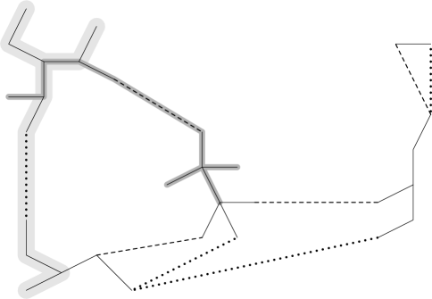
Bi-trees of spheromorphisms. See Fig. 4. Let $\{S_{\alpha}\}$ be the perfect $(\mathbb{T})$-covering forest for a spheromorphism $g$. Consider the skeleton $\mathop{\mathrm{Skel}}\nolimits\{S_{\alpha}\}$ of $\{S_{\alpha}\}$, it is a tree with black and blue edges. Consider also the skeleton $\mathop{\mathrm{Skel}}\nolimits\{gS_{\alpha}\}$ of $\{gS_{\alpha}\}$, let us color it black and red (instead of blue). For each $S_{j}$ consider the minimal subtree $\Xi_{j}$ in $S_{j}$ containing the subtrees

$$S_{j}\cap\mathop{\mathrm{Skel}}\nolimits\{S_{\alpha}\},\qquad g^{-1}\bigl{(}gS_{j}\cap\mathop{\mathrm{Skel}}\nolimits\{gS_{\alpha}\}\bigr{)}.$$

We have embeddings of subtrees

$$\begin{array}[]{ccl}&&\Xi_{j}\\ &\nearrow&\\ \Xi_{j}\cap\mathop{\mathrm{Skel}}\nolimits\{S_{\alpha}\}&&\\ &\searrow&\\ &&\mathop{\mathrm{Skel}}\nolimits\{S_{\alpha}\}\end{array},\qquad\begin{array}[]{ccl}&&\Xi_{j}\\ &\nearrow&\\ \Xi_{j}\cap g^{-1}\mathop{\mathrm{Skel}}\nolimits\{gS_{\alpha}\}&&\\ &\searrow&\\ &&\mathop{\mathrm{Skel}}\nolimits\{gS_{\alpha}\}\end{array}.$$

We glue together trees $\Xi_{1}$, $\Xi_{2}$, …, $\mathop{\mathrm{Skel}}\nolimits\{S_{\alpha}\}$, $\mathop{\mathrm{Skel}}\nolimits\{gS_{\alpha}\}$ identifying images of subtrees $\Xi_{j}\cap\mathop{\mathrm{Skel}}\nolimits\{S_{\alpha}\}$ and $\Xi_{j}\cap g^{-1}\mathop{\mathrm{Skel}}\nolimits\{gS_{\alpha}\}$ in the target-spaces and get a graph $\Gamma(g)$, we call it the bi-tree of the spheromorphism $g$.

Refer to caption

Notation: Refer to caption – black, Refer to caption – blue, Refer to caption – red. Thin lines Refer to caption are auxiliary (and are not elements of graphs).

Figure 4: Ref to Subsect. 2. Skeletons $\mathop{\mathrm{Skel}}\nolimits\{S_{\alpha}\}$ and $\mathop{\mathrm{Skel}}\nolimits\{gS_{\alpha}\}$ and the corresponding bi-tree drawn in the ’horizontal’ plane.

Formulate the last step in a simpler way. Consider the forest $\{\Xi_{\alpha}\}$. Consider a blue edge in $\mathop{\mathrm{Skel}}\nolimits\{S_{\alpha}\}$. It has two ends, which are vertices of different $\Xi_{i}$, $\Xi_{j}$. We connect these vertices by a blue edge. Repeat the same procedure for red edges131313We can not receive a double blue-red edges, otherwise a $(\mathbb{T})$-covering forest $\{S_{\alpha}\}$ is not perfect..

Remark. By construction, both skeletons $\mathop{\mathrm{Skel}}\nolimits\{S_{\alpha}\}$, $\mathop{\mathrm{Skel}}\nolimits\{gS_{\alpha}\}$ are embedded to $\Gamma(g)$. $\boxtimes$

Construction of a double coset $\in\mathop{\mathrm{Aut}}\nolimits(\mathbb{T})\setminus\mathop{\mathrm{Hier}}\nolimits(\mathbb{T})/\mathop{\mathrm{Aut}}\nolimits(\mathbb{T})$ from a bi-tree $\Gamma$. Take two copies $\mathbb{T}_{1}$, $\mathbb{T}_{2}$ of tree $\mathbb{T}$. Choose isomorphisms $\theta_{1,2}:\mathbb{T}\to\mathbb{T}_{1,2}$. Consider embeddings

$$p:\Gamma^{\mathrm{black}}_{\mathrm{blue}}\to\mathbb{T}_{1},\qquad q:\Gamma^{\mathrm{black}}_{\mathrm{red}}\to\mathbb{T}_{2}.$$

Then $p$ (resp. $q$) determines a $(\mathbb{T})$-covering forest (we remove images of blue edges from $\mathbb{T}$), say $\{P_{\alpha}\}$ (say $\{Q_{\alpha}\}$). The set of components of $\{P_{\alpha}\}$ (resp. $\{Q_{\alpha}\}$) is in a one-to-one correspondence with the set of components $\{\Xi_{\alpha}\}$ of $\Gamma^{\mathrm{black}}$. For each $P_{j}$ we restrict $p$ to $\Gamma^{\mathrm{black}}_{\mathrm{blue}}\cap\Xi_{j}$ and get an embedding of this tree to $P_{j}$. Extend it to an embedding $\widetilde{p}_{j}:\Xi_{j}\to P_{j}$. In the same way we get embeddings $\widetilde{q}_{j}:\Xi_{j}\to Q_{j}$. Finally, we choose isomorphisms $\widetilde{r}_{j}:P_{j}\to Q_{j}$ such that $\widetilde{q}_{j}=\widetilde{r}_{j}\circ\widetilde{p}_{j}$. Thus we get a spheromorphism $r:=\{\widetilde{r}_{j}\}:\mathbb{T}_{1}\to\mathbb{T}_{2}$ and define a spheromorphism $g:\mathbb{T}\to\mathbb{T}$ as

$$g=\theta_{2}^{-1}\circ r\circ\theta_{1}.$$

2.5. A $(G,K)$-pair related to symmetric groups. Let $\Omega$ be a countable set. Denote by $S(\Omega)$ the group of all permutations of $\Omega$. The topology on $S(\Omega)$ is determined from the condition: stabilizers of finite subsets in $\Omega$ are open subgroups. This determines a structure of a Polish group on $S(\Omega)$. On the other hand (see [9]) it is a unique separable topology on the full infinite symmetric group (in particular, all unitary representations of this group are automatically continuous in our topology). We also write $S_{\infty}$ if we do not wish to indicate the set $\Omega$.

Denote by $S^{\mathrm{fin}}(\Omega)=S^{\mathrm{fin}}_{\infty}$ the subgroup of finitely supported permutations of $\Omega$, it is a countable group equipped with the discrete topology.

Let $A$ and $B$ be disjoint countable sets. Denote by $S(A\bigl{|}B)$ the subgroup in $S(A\sqcup B)$ generated by $S(A)\times S(B)$ and $S^{\mathrm{fin}}(A\sqcup B)$. In notation of [23], [16] it is a $(G,K)$-pair

$$\bigl{(}S_{2\infty},S_{\infty}\times S_{\infty}).$$

Unitary representations of this $(G,K)$-pair were classified by Olshanski [23].

For any element $\sigma$ of $S(A\bigl{|}B)$ there is a number $k$ such that $\sigma$ sends precisely $k$ elements of $A$ to $B$ and $k$ elements of $B$ to $A$ (this property can be regarded as a definition of our group).

The homogeneous space

$$\Omega:=S(A\bigl{|}B)\bigr{/}(S(A)\times S(B))$$

is countable. It can be identified with the set of all subsets $U\subset A\sqcup B$ such that the sets $A\setminus U$ and $U\setminus A$ are finite and contain the same number of elements.

We define the topology on $S(A\bigl{|}B)$ from the assumptions:

$\bullet$ the induced topology on $S(A)\times S(B)$ is the natural topology on this subgroup.

$\bullet$ the topology on the homogeneous space $S(A\bigl{|}B)\bigr{/}(S(A)\times S(B))$ is discrete.

It is clear that we get a Polish group.

Remark. The group $S(A\bigl{|}B)$ acts in $\ell^{2}(\Omega)$ and the topology of $S(A\bigl{|}B)$ is induced from the unitary group of $\ell^{2}(\Omega)$. $\boxtimes$

2.6. The topology on $\mathop{\mathrm{Hier}}\nolimits(\mathbb{T})$. The group $\mathop{\mathrm{Aut}}\nolimits(\mathbb{T})$ acts on the set $\mathop{\mathrm{vert}}\nolimits(\mathbb{T})$ of vertices of the tree, therefore we get an embedding $\mathop{\mathrm{Aut}}\nolimits(\mathbb{T})\to S\bigl{(}\mathop{\mathrm{vert}}\nolimits(\mathbb{T})\bigr{)}$. The topology on $\mathop{\mathrm{Aut}}\nolimits(\mathbb{T})$ defined above is induced from the symmetric group $S\bigl{(}\mathop{\mathrm{vert}}\nolimits(\mathbb{T})\bigr{)}$.

Next, we define a topology on $\mathop{\mathrm{Hier}}\nolimits(\mathbb{T})$ from the following two conditions:

A) the induced topology on $\mathop{\mathrm{Aut}}\nolimits(\mathbb{T})$ coincides with the natural topology on $\mathop{\mathrm{Aut}}\nolimits(\mathbb{T})$.

B) this topology is a strongest topology satisfying the property A.

In particular, a homomorphism from $\mathop{\mathrm{Hier}}\nolimits(\mathbb{T})$ to a topological group is continuous if and only if it is continuous on the subgroup $\mathop{\mathrm{Aut}}\nolimits(\mathbb{T})$.

Proposition 2.2

a) The topology satisfying the properties A–B exists and the (countable) homogeneous space $\mathop{\mathrm{Hier}}\nolimits(\mathbb{T})/\mathop{\mathrm{Aut}}\nolimits(\mathbb{T})$ has the discrete topology.

b) The group $\mathop{\mathrm{Hier}}\nolimits(\mathbb{T})$ is Polish.

To observe this, we consider the set $C$ of all non-ordered pairs $(u,v)$, where $u$, $v\in\mathop{\mathrm{vert}}\nolimits(\mathbb{T})$, uβ‰ v𝑒𝑣u\neq v. We put $(u,v)$ to a set $A$ if $u$, $v$ are connected by an edge and to $B$ otherwise. An spheromorphism $g\in\mathop{\mathrm{Hier}}\nolimits(\mathbb{T})$ acts on $C$ sending $(u,v)$ to $(gu,gv)$. Clearly, we have a homomorphism

$$\mathop{\mathrm{Hier}}\nolimits(\mathbb{T})\to S(A\bigl{|}B)$$

sending $\mathop{\mathrm{Aut}}\nolimits(\mathbb{T})$ to $S(A)\times S(B)$. Moreover, $\mathop{\mathrm{Aut}}\nolimits(\mathbb{T})$ is precisely the preimage of $S(A)\times S(B)$. This implies the statement a).

On the other hand the image of $\mathop{\mathrm{Hier}}\nolimits(\mathbb{T})$ is closed in $S(A\bigl{|}B)$ and a closed subgroup of a Polish group is Polish.

2.7. The ball-algebra $\mathcal{A}$.

Lemma 2.3

Let $S_{1}$, $S_{2}$ be $(\mathbb{T})$-subtrees of $\mathbb{T}$.

a) If $S_{1}\cap S_{2}$ is not empty, then it is a $(\mathbb{T})$-subtree.

a) If $S_{1}\setminus S_{2}$ is not empty, then $\mathop{\mathrm{vert}}\nolimits(S_{1})\setminus\mathop{\mathrm{vert}}\nolimits(S_{2})$ is a set of vertices of a forest consisting of $(\mathbb{T})$-subtrees.

This is obvious.

Removing an edge of $\mathbb{T}$ we get two $(\mathbb{T})$-subtrees. We call them branches. We call a subset of the boundary $\partial\mathbb{T}$ adjacent to a branch a ball141414Let us use notation of Subsect..Β 1. Consider a branch that do not cantain the initial point of $\mathbb{T}$. Then the adjoint subset of the boundary is a ball in the sense of the metric $d_{\boldsymbol{\cdot}}$.. Consider the algebra151515We say that a family $\mathcal{A}$ of subsets of a set $X$ is an algebra if $B\in\mathcal{A}$ implies that $X\setminus B\in\mathcal{A}$ and $B$, $C\in\mathcal{A}$ implies $B\cap C$, $B\cup C\in\mathcal{A}$. $\mathcal{A}(\mathbb{T})$ of subsets in $\mathop{\mathrm{vert}}\nolimits(\mathbb{T})$ generated by all branches. By $\mathcal{A}(\partial\mathbb{T})$ denote the algebra of subsets in $\partial\mathbb{T}$ generated by all balls.

Lemma 2.4

a) Any element of $\mathcal{A}(\mathbb{T})$ is a set of vertices of a forest $S_{1}$, …, $S_{k}$ consisting of $(\mathbb{T})$-subtrees.

b) The algebra $\mathcal{A}(\mathbb{T})$ is countable.

c) The map sending $R\in\mathcal{A}(\mathbb{T})$ to its boundary is an isomorphism of algebras $\mathcal{A}(\mathbb{T})$ and $\mathcal{A}(\partial\mathbb{T})$.

d) Sets $B\in\mathcal{A}(\partial\mathbb{T})$ are closed and open.

e) The group $\mathop{\mathrm{Hier}}\nolimits(\mathbb{T})$ acts on the set of nontrivial elements of $\mathcal{A}$ transitively.

Proof. Proofs of a)-d) are obvious. Let us prove e). Let $S_{1}$, …, $S_{k}\subset\mathbb{T}$ and $S_{1}^{\prime}$, …, $S_{k^{\prime}}\subset\mathbb{T}$ be two forests of $(\mathbb{T})$-subtrees. Denote by $T_{1}$, …, $T_{m}$ and $T_{1}^{\prime}$, …, $T_{m^{\prime}}^{\prime}$ the complementary forests. We can subdivide any $(\mathbb{T})$-subtree to several $(\mathbb{T})$-subtrees, therefore we can assume $k^{\prime}=k$, $m^{\prime}=m$. Now we take a spheromorphism sending $S_{j}\to S_{j}^{\prime}$, $T_{i}\to T_{i}^{\prime}$. $\square$

3 The Baire space and the Thompson group

3.1. The correspondence between ${\mathbb{R}}\setminus{\mathbb{Q}}$ and $\partial\mathbb{T}$. Let $y_{1}$, $y_{2}\in{\mathbb{Q}}$. Denote

$$(\!(y_{1},y_{2})\!):=(y_{1},y_{2})\cap{\mathbb{Q}}.$$

Cut ${\mathbb{R}}\setminus{\mathbb{Q}}={\mathbb{R}}\mathbb{P}^{1}\setminus{\mathbb{Q}}\mathbb{P}^{1}$ into 4 pieces $(\!(-\infty,-1)\!)$, $(\!(-1,0)\!)$, $(\!(0,1)\!)$, $(\!(1,\infty)\!)$. We represent points $x$ of these sets as continued fractions

$\displaystyle(\!(-\infty,-1)\!)$ $\displaystyle:\quad x=-[s_{0};s_{1};s_{2};\dots];$
$\displaystyle(\!(-1,0)\!)$ $\displaystyle:\quad x=-[0;s_{1};s_{2};\dots];$
$\displaystyle(\!(0,1)\!)$ $\displaystyle:\quad x=[0;s_{1};s_{2};\dots];$
$\displaystyle(\!(1,\infty)\!)$ $\displaystyle:\quad x=[s_{0};s_{1};s_{2};\dots].$

In all cases $s_{j}\in{\mathbb{N}}$. For definiteness, consider $(\!(0,1)\!)$. We consider a tree whose vertices are enumerated by collections (s1,…,sk)subscript𝑠1…subscriptπ‘ π‘˜(s_{1},\dots,s_{k}), edges have a form

$(s_{1},\dots,s_{k-1}$) β€” (s1,…,skβˆ’1,sk)subscript𝑠1…subscriptπ‘ π‘˜1subscriptπ‘ π‘˜(s_{1},\dots,s_{k-1},s_{k}). (3.1)

We get a tree isomorphic to $\mathbb{T}$, and the boundary of this tree is identified with $(\!(0,1)\!)$.

So we get 4 copies of the tree $\mathbb{T}$. Adding 3 edges connecting their initial points we unite them to one tree $\mathbb{T}$, the boundary of this tree is in one-to-one correspondence with ${\mathbb{R}}\setminus{\mathbb{Q}}$. Thus we get the map

$$\Xi:{\mathbb{R}}\setminus{\mathbb{Q}}\to\partial\mathbb{T}.$$

Consider the algebra $\mathcal{R}$ of subsets in ${\mathbb{R}}\setminus{\mathbb{Q}}$ generated by all intervals $(\!(u,v)\!)$ with rational $u$, $v$ (we admit $u=-\infty$ and $v=\infty$). On the other hand, we have the algebra

$$\mathcal{A}(\mathbb{B}):=\mathcal{A}(\partial\mathbb{T}).$$
Proposition 3.1

The map $\Xi$ determines a bijection between algebras $\mathcal{R}$ and $\mathcal{A}(\mathbb{B})$.

Proof. It is sufficient to show that any ball in $\partial\mathbb{T}$ corresponds to an element of $\mathcal{R}$ and any interval $(\!(u,v)\!)$ corresponds to an element of $\mathcal{A}$.

1) For definiteness let us remove an edge (3.1) in the $(\mathbb{T})$-subtree corresponding to $(\!(0,1)\!)$. We get two branches of $\mathbb{T}$, one of them is completely contained in the subtree. Its boundary consists of points

[0;s0,…,sk,tk+1,tk+2,…],whereΒ tmΒ range inΒ β„•.0subscript𝑠0…subscriptπ‘ π‘˜subscriptπ‘‘π‘˜1subscriptπ‘‘π‘˜2…whereΒ tmΒ range inΒ β„•.[0;s_{0},\dots,s_{k},t_{k+1},t_{k+2},\dots],\quad\text{where $t_{m}$ range in ${\mathbb{N}}$.}

In other words, we get the interval

$$\Bigl{(}\!\!\Bigr{(}[0;s_{0},\dots,s_{k}],[0;s_{0},\dots,s_{k}+1]\Bigl{)}\!\!\Bigr{)}\quad\text{or}\quad\Bigl{(}\!\!\Bigr{(}[0;s_{0},\dots,s_{k}+1],[0;s_{0},\dots,s_{k}]\Bigl{)}\!\!\Bigr{)}$$

depending of the parity of $k$.

2) Conversely, consider an interval $(\!(u,v)\!)$, where $0\leqslant u<v\leqslant 1$. We have $(\!(u,v)\!)=(\!(0,w)\!)\cap(\!(v,1)\!)$. For definiteness consider the subset of the Baire space corresponding to $(\!(0,w)\!)$. Decompose $w$ into a continued fraction,

w:=[0;s1,…,sk].assign𝑀0subscript𝑠1…subscriptπ‘ π‘˜w:=[0;s_{1},\dots,s_{k}].

Let $k=1$. Then

$$(\!(0,w)\!)=\bigl{(}\!\bigr{(}0,\tfrac{1}{s_{1}}\bigl{)}\!\bigr{)}=(\!(0,1)\!)\setminus\bigcup_{j=1}^{s_{1}-1}\bigl{(}\!\bigr{(}\tfrac{1}{j+1},\tfrac{1}{j}\bigl{)}\!\bigr{)}=(\!(0,1)\!)\setminus\bigcup_{j=1}^{s_{1}-1}\bigl{(}\!\bigr{(}\,[0;j+1],[0;j]\,\bigl{)}\!\bigr{)}.$$

Let $k$ be even. We represent our interval as

$$\bigl{(}\!\bigr{(}0,[0,s_{1},\dots,s_{k-1},s_{k}]\bigl{)}\!\bigr{)}=\bigl{(}\!\bigr{(}0,[0,s_{1},\dots,s_{k-1}]\bigl{)}\!\bigr{)}\\ \bigcup\bigcup_{j=1}^{s_{k}-1}\bigl{(}\!\bigr{(}\,[s_{1},\dots,s_{k-1}+j],[s_{1},\dots,s_{k-1}+j+1]\,\bigl{)}\!\bigr{)}.$$

For odd $k>1$ we write

$$\bigl{(}\!\bigr{(}0,[0,s_{1},\dots,s_{k-1},s_{k}]\bigl{)}\!\bigr{)}=\bigl{(}\!\bigr{(}0,[0,s_{1},\dots,s_{k-1}]\bigl{)}\!\bigr{)}\\ \bigl{\backslash}\bigcup_{j=1}^{s_{k}-1}\bigl{(}\!\bigr{(}\,[s_{1},\dots,s_{k-1}+j+1],[s_{1},\dots,s_{k-1}+j]\,\bigl{)}\!\bigr{)}.$$

In all cases we have get an interval $(\!(0,w^{\prime})\!)$, where a continued fraction for $w^{\prime}$ is shorter than the a continued fraction for $w$, and a collection of intervals $(\!(p_{j},q_{j})\!)$ corresponding to balls in $\partial\mathbb{T}$. So we can apply the induction. $\square$

3.2. The action of the Thompson group.

Theorem 3.2

Let $\varkappa$ be a transformation of ${\mathbb{R}}\setminus{\mathbb{Q}}$ lying in the Thompson group $\mathrm{T\!h}$. Then $\Xi\circ\varkappa\circ\Xi^{-1}$ is contained in $\mathop{\mathrm{Hier}}\nolimits(\mathbb{T})$.

Recall that the group $\mathop{\mathrm{PGL}}\nolimits_{2}({\mathbb{Z}})$ acts on ${\mathbb{R}}\setminus{\mathbb{Q}}$ by linear fractional transformations. First, we prove the following preliminary statement.

Proposition 3.3

For any $h\in\mathop{\mathrm{PGL}}\nolimits_{2}({\mathbb{Z}})$ we have $\Xi\circ h\circ\Xi^{-1}\in\mathop{\mathrm{Hier}}\nolimits(\mathbb{T})$.

Proof. It is sufficient to prove this statement for generators

$$\begin{pmatrix}0&1\\ 1&0\end{pmatrix}:\quad x\mapsto\frac{1}{x};\qquad\begin{pmatrix}1&1\\ 0&1\end{pmatrix}:\quad x\mapsto x+1$$

of the group $\mathop{\mathrm{PGL}}\nolimits_{2}({\mathbb{Z}})$.

a) Let $x\in(\!(0,1)\!)$,

$$x=[0;s_{1},s_{2},s_{3},\dots].$$

Then

$$x^{-1}=[s_{1};s_{2},s_{3},\dots]$$

and we permute branches $\Xi(\!(0,1)\!)$ and $\Xi(\!(1,\infty)\!)$ preserving their structures. The same holds for $(\!(-1,0)\!)$ and $(\!(-\infty,-1)\!)$.

b) Examine the transformation $x\mapsto x+1$.

b.1) Let $x\in(\!(-\infty,-2)\!)$,

$$x=-[s_{0};s_{1},s_{2},\dots],\quad x+1=-[s_{0}-1;s_{1},s_{2},\dots].$$

Transformation of subtrees corresponding to the shift $(\!(-\infty,-2)\!)\to(\!(-\infty,-1)\!)$ is shown on Fig. 5.

Refer to caption
Figure 5: Ref. to the proof of Proposition 3.3. The shift $(\!((-\infty,-2)\!)\to(\!((-\infty,-1)\!)$.

b.2) The map $(\!(-2,-1)\!)\to(\!(-1,0)\!)$. We send $x=[-1;s_{1},s_{2},\dots]$ to $x=[0;s_{1},s_{2},\dots]$. This is an isomorphic map of two branches of $\mathbb{T}$.

b.3) Let $x\in(\!(-1,0)\!)$. We represent it in two forms

$\displaystyle x=-[0;s_{1},s_{2},\dots]$ $\displaystyle=-\frac{1}{s_{1}+\eta},\qquad\text{where $0<\eta<1$},$
$\displaystyle=-\cfrac{1}{s_{1}+\cfrac{1}{s_{2}+\xi}},\qquad\text{where $0<\xi<1$.}$

Let $s_{1}>1$. Then

$$-x+1=-\frac{1}{s_{1}+\eta}+1=\frac{s_{1}-1+\eta}{1+\eta}=\cfrac{1}{1+\cfrac{1}{s_{1}-1+\eta}}.$$

For $s_{1}=1$ we have

$$-x+1=-\cfrac{1}{1+\cfrac{1}{s_{2}+\xi}}+1=\cfrac{1}{s_{2}+1+\xi}.$$

The correspondence of branches is shown on Fig. 6.

Refer to caption
Figure 6: Ref. to the proof of Proposition 3.3. The shift $(\!(-1,0)\!)\to(\!(0,1)\!)$.

b.4) The examination of the shift $x\mapsto x+1$ on $(\!(0,1)\!)$, $(\!(1,\infty)\!)$ is similar to the case b.1). $\square$

Proof of Theorem 3.2. Consider a piece-wise $\mathop{\mathrm{PSL}}\nolimits_{2}({\mathbb{Z}})$-transformation $h$ of ${\mathbb{R}}\mathbb{P}^{1}$. The projective line is a union of of rational segments $[r_{m},r_{m+1}]$, on which the transformation corresponds to some elements $\gamma_{m}\in\mathop{\mathrm{PSL}}\nolimits_{2}({\mathbb{Z}})$. Such segments $[r_{m},r_{m+1}]$ correspond to elements $B_{m}$ of the algebra $\mathcal{A}$, for each element we have a finite collection $S_{m1}$, $S_{m2}$, …of $(\mathbb{T})$-subtrees. On the other hand $\gamma_{m}$ determines a spheromorphism and therefore a finite collection of $R_{m1}$, $R_{m2}$, $\dots$ of $(\mathbb{T})$-subtrees. Therefore

$$U_{mij}:=S_{mi}\cap R_{mj}$$

is a splitting of $\mathbb{T}$ into $(\mathbb{T})$-subtrees and $\Xi\circ h\circ\Xi^{-1}$ embeds each subtree to $\mathbb{T}$. $\square$

4 The train of the group $\mathop{\mathrm{Hier}}\nolimits(\mathbb{T})$

4.1. Double cosets and combinatorial data. For a non-empty finite subtree $J\subset\mathbb{T}$ denote by $\mathcal{K}(J)\subset\mathop{\mathrm{Aut}}\nolimits(\mathbb{T})$ the pointwise stabilizer of $J$. We wish to describe spaces of double cosets

$$\mathcal{K}(J)\setminus\mathop{\mathrm{Hier}}\nolimits(\mathbb{T})/\mathcal{K}(I)$$

for finite nonempty subtrees $I$, $J$.

Consider a graph $\Gamma$ whose edges are colored black, blue, and red. Denote by $\Gamma^{\mathrm{black}}$ the subgraph consisting of black edges, by $\Gamma^{\mathrm{black}}_{\mathrm{blue}}$ of black and blue edges, by $\Gamma^{\mathrm{black}}_{\mathrm{red}}$ of black and red edges.

Let $\Gamma$ be such a graph equipped with embeddings $\imath:I\to\Gamma$, $\jmath:J\to\Gamma$. We say that $(\Gamma,\imath,\jmath)$ is a $(I,J)$-bi-tree if the following conditions hold:

$\bullet$ the subgraphs $\Gamma^{\mathrm{black}}_{\mathrm{blue}}$ and $\Gamma^{\mathrm{black}}_{\mathrm{red}}$ are trees;

$\bullet$ $\imath(I)\subset\Gamma^{\mathrm{black}}_{\mathrm{blue}}$, $\jmath(J)\subset\Gamma^{\mathrm{black}}_{\mathrm{red}}$;

$\bullet$ any vertex of $\Gamma$ of valence 1 is an end of a black edge contained in $\imath(I)$ or $\imath(J)$.

Refer to caption

Notation: Refer to caption is black, Refer to caption is blue, Refer to caption is red,
edges Refer to caption are in $\imath(I)$, Refer to caption are in $\jmath(J)$.

Figure 7: Ref. to Subsect. 4. An $(I,J)$-bi-tree. Removing blue and red edges we get a black forest consisting of 4 trees.

Two $(I,J)$-bi-trees $(\Gamma,\imath,\jmath)$ and $(\Gamma^{\prime},\imath^{\prime},\jmath^{\prime})$ are equivalent if there is a color preserving isomorphism $\lambda:\Gamma\to\Gamma^{\prime}$ such that $\imath^{\prime}=\lambda\circ\imath$, $\jmath^{\prime}=\lambda\circ\jmath$.

Proposition 4.1

There is a canonical one-to-one correspondence between the space $\mathcal{K}(I)\setminus\mathop{\mathrm{Hier}}\nolimits(\mathbb{T})/\mathcal{K}(J)$ of double cosets and the set of all $(I,J)$-bi-trees defined upto the equivalence.

This is version of the correspondence defined in Subsect. 2.

Construction of an $(I,J)$-bi-tree by a spheromorphism $g$. Fix $g\in\mathop{\mathrm{Hier}}\nolimits(\mathbb{T})$. Consider the perfect $(\mathbb{T})$-covering forest $\{S_{\alpha}\}$ compatible with $g$, see Subsect. 2. Paint blue all edges in $\mathbb{T}\setminus\bigcup S_{j}$. The $I$-skeleton $\mathop{\mathrm{Skel}}\nolimits_{I}\{S_{\alpha}\}$ of $\{S_{\alpha}\}$ is the minimal subgraph in $\mathbb{T}$ containing all blue edges and $I$. Next, we paint red all edges of $\mathbb{T}\setminus\bigcup gS_{j}$, and consider $J$-skeleton of $\{gS_{\alpha}\}$, i.Β e., the minimal subgraph in $\mathbb{T}$ containing red edges and $J$.

In each $S_{k}$ we have two subtrees, $S_{k}\cap\mathop{\mathrm{Skel}}\nolimits_{I}(\{S_{\alpha}\})$ and $g^{-1}(gS_{k}\cap\mathop{\mathrm{Skel}}\nolimits_{J}(\{gS_{\alpha}\}))$. Consider the minimal subtree $\Xi_{k}$ containing these subtrees and paint it black. Any blue edge in $\mathop{\mathrm{Skel}}\nolimits_{I}(\{S_{\alpha}\})$ has two ends in some $S_{k}$, $S_{m}$. These ends are contained in $\Xi_{k}$, $\Xi_{m}$. So we add blue edges to the forest $\{\Xi_{\alpha}\}$, in the same way we add red edges.

Since our $(\mathbb{T})$-covering forest is perfect, we do not get double red-blue edges.

Remark. For a given spheromorphism $g$ we have a canonical embedding $i_{+}$ of $\Gamma^{\mathrm{black}}_{\mathrm{blue}}$ to $\mathbb{T}$ and a canonical embedding $i_{-}$ of $\Gamma^{\mathrm{black}}_{\mathrm{red}}$ to $\mathbb{T}$. They are related by

$$i_{-}\Bigr{|}_{\Gamma^{\mathrm{black}}}=g\circ i_{+}\Bigr{|}_{\Gamma^{\mathrm{black}}}$$

We denote these subtrees in $\mathbb{T}$ by ${}^{*}\Gamma^{\mathrm{black}}_{\mathrm{blue}}$ and ${}^{*}\Gamma^{\mathrm{black}}_{\mathrm{red}}$. $\square$

The inverse construction. Let $\Gamma$ be an $(I,J)$-bi-tree. Take two copies $\mathbb{T}_{1}$, $\mathbb{T}_{2}$ of the tree $\mathbb{T}$ with $I$ drawn on $\mathbb{T}_{1}$ and $J$ drawn on $\mathbb{T}_{2}$. Choose isomorphisms $\theta_{1,2}:\mathbb{T}\to\mathbb{T}_{1,2}$. Consider embeddings

$$p:\Gamma^{\mathrm{black}}_{\mathrm{blue}}\to\mathbb{T}_{1},\qquad q:\Gamma^{\mathrm{black}}_{\mathrm{red}}\to\mathbb{T}_{2}$$

such that

$$\theta^{-1}_{1}\circ p\circ\imath,\quad\theta^{-1}_{2}\circ q\circ\jmath$$

are identical maps $I\to I$ and $J\to J$ respectively.

Then $p$ determines a $(\mathbb{T})$-covering forest, say $\{P_{\alpha}\}$, of $\mathbb{T}_{1}$ (we remove images of blue edges from $\mathbb{T}_{1}$). In the same way $q$ determines a $(\mathbb{T})$-covering forest, say $\{Q_{\alpha}\}$, of $\mathbb{T}_{2}$.

The set of components of $\{P_{\alpha}\}$ (resp., $\{Q_{\alpha}\}$) is in a one-to-one correspondence with the set of components $\{\Xi_{\alpha}\}$ of the black forest $\Gamma^{\mathrm{black}}$. For each $P_{k}$ we restrict $p$ to $\Gamma^{\mathrm{black}}_{\mathrm{blue}}\cap\Xi_{k}$ and get an embedding of this tree to $P_{k}$. Extend it to an embedding $\widetilde{p}_{k}:\Xi_{j}\to P_{k}$.

In the same way we get embeddings $\widetilde{q}_{j}:\Xi_{j}\to Q_{j}$. Next, we choose isomorphisms $\widehat{r}_{j}:P_{j}\to Q_{j}$ such that

$$\widetilde{q}_{j}\Bigr{|}_{\Xi_{j}}=\widehat{r}_{j}\circ\widetilde{p}_{j}\Bigr{|}_{\Xi_{j}}.$$

This determines a spheromorphism $r:=\{\widehat{r}_{j}\}:\mathbb{T}_{1}\to\mathbb{T}_{2}$ and a spheromorphism $g:\mathbb{T}\to\mathbb{T}$

$$g=\theta_{2}^{-1}\circ r\circ\theta_{1}.$$

Multiplying $\theta_{1}\mapsto\theta_{1}h_{1}$, $\theta_{2}\mapsto\theta_{2}h_{2}$, where $h_{1}\in\mathcal{K}(I)$, $h_{2}\in\mathcal{K}(J)$, we get all elements of the double coset.

On the other hand maps $\widehat{r}_{k}$ are not canonical and they can be replaced by maps $\widehat{r}_{k}\circ\zeta_{k}$, where $\zeta_{k}$ are maps $P_{k}\to P_{k}$ fixing $\Xi_{k}$. This determines a spheromorphism $\{\zeta_{k}\}$, which is contained in $\mathop{\mathrm{Aut}}\nolimits(\mathbb{T})$. Now we can replace $\theta_{1}$ by $\{\zeta_{k}\}\circ\theta_{1}=\theta_{1}\circ(\theta_{1}^{-1}\circ\{\zeta_{k}\}\circ\theta_{1})$ and we get an element of the same double coset.

Weak bi-trees of spheromorphisms. In proof of Lemma 4.6 we need a variation of the construction. Consider the following data: a spheromorphism $g$, a compatible $(\mathbb{T})$-covering forest $\{S_{\alpha}\}$ (generally, non-perfect) and a collection $\{v_{j}\}$ of marked vertices in $\mathbb{T}$. Then we apply the procedure of drawing of a bi-tree and get the graph $\varGamma$ whose edges are colored black, blue, red, and double blue-red edges are allowed. We define the subgraph $\varGamma^{\mathrm{black}}_{\mathrm{blue}}$ as the graph obtained by removing red edges (double blue-red edge become blue). In a similar way we define the subgraph $\varGamma^{\mathrm{black}}_{\mathrm{red}}$. Again, $\varGamma^{\mathrm{black}}_{\mathrm{blue}}$, $\varGamma^{\mathrm{black}}_{\mathrm{red}}$ are trees, whose terminal black edges finish at marked points.

4.2. The category of bi-trees and the category of double cosets. Denote by $\mathcal{M}(I,J)$ the set of $(I,J)$-bi-trees. We wish to define a product

$$\mathcal{M}(J_{1},J_{2})\times\mathcal{M}(J_{2},J_{3})\to\mathcal{M}(J_{1},J_{3}).$$

Let $\Gamma\in\mathcal{M}(J_{2},J_{3})$, $\Delta\in\mathcal{M}(J_{1},J_{2})$. We glue $\Gamma$ and $\Delta$ identifying images of embeddings $J_{2}\to\Gamma$, $J_{2}\to\Delta$, see Fig.8. After this we can get double colors on some edges of $J_{2}$. We replace161616We indicate both color of an edge and the origin of an edge ($\Delta$ or $\Gamma$).

(Ξ”-blue,Β Ξ“-black)⟢(blue),(Β Ξ”-black,Β Ξ“-red)⟢(red)formulae-sequence⟢(Ξ”-blue,Β Ξ“-black)(blue)⟢(Β Ξ”-black,Β Ξ“-red)(red)\text{($\Delta$-blue, $\Gamma$-black)}\longrightarrow\text{(blue)},\quad\text{( $\Delta$-black, $\Gamma$-red)}\longrightarrow\text{(red)}

and remove ($\Delta$-blue, $\Gamma$-red)-edges171717We also have ($\Delta$-black, $\Gamma$-black)$\longrightarrow$ (black), other combinations of colors are impossible.. Finally, remove all vertices of valence 1, that are not contained in the images of $J_{1}$ and $J_{3}$ (such vertices are automatically contained in $J_{2}$ and adjacent edges are black). Repeat the step again, etc181818A black edge survives if and only if it can be included to a way $v_{1},\dots,v_{m}$ following black edges, whose terminal vertices $v_{1}$, $v_{m}$ are contained in $J_{1}$, $J_{3}$ or are ends of blue or red edges..

Lemma 4.2

In this way, we get a $(J_{1},J_{3})$-bi-tree.

Refer to caption
Figure 8: Refs. to Subsect. 4 and Lemma 4.4. Gluing of bi-trees.

Denote this $(J_{1},J_{3})$-bi-tree by $\Delta\diamond\Gamma$.

Proof. Let us examine the graph $\Theta$ obtained by glueing of $\Delta$ and $\Gamma$. Consider its subgraph consisting of edges, on which black or red are present191919Recall that some edges have two colors., i.e., $\Delta^{\mathrm{black}}_{\mathrm{red}}\cup\Gamma^{\mathrm{black}}_{\mathrm{red}}$. The subtree $\Gamma^{\mathrm{black}}_{\mathrm{red}}$ contains $J_{2}$. The graph $\Delta^{\mathrm{black}}_{\mathrm{red}}\setminus\{\mathop{\mathrm{edge}}\nolimits(J_{2})\}$ is a forest and each component has one or two vertices in $\mathop{\mathrm{vert}}\nolimits(J_{2})$. Consider an edge $[v,w]$ of $J_{2}$. There are two cases:

1) The edge $[v,w]$ is black in $\Delta$. This edge is a unique way in $\Delta^{\mathrm{black}}_{\mathrm{red}}$ connecting $v$ and $w$. Since $\Gamma^{\mathrm{black}}_{\mathrm{red}}\supset J_{2}$ can be contracted to $J_{2}$, then $[v,w]$ is a unique way in $\Delta^{\mathrm{black}}_{\mathrm{red}}\cup\Gamma^{\mathrm{black}}_{\mathrm{red}}$ connecting $v$ and $w$.

2) The edge $[v,w]$ is blue in $\Delta$. According our rules it is blue in $\Delta\diamond\Gamma$ and absent in $[\Delta\diamond\Gamma]^{\mathrm{black}}_{\mathrm{red}}$. However, the vertices $v$ and $w$ are connected by a unique way in $\Delta^{\mathrm{black}}_{\mathrm{red}}$, and this way is contained in $[\Delta\diamond\Gamma]^{\mathrm{black}}_{\mathrm{red}}$.

The same argument holds for $[\Delta\diamond\Gamma]^{\mathrm{black}}_{\mathrm{blue}}$.

Next, all edges of $J_{2}\cap J_{3}$ and of $J_{1}\cap J_{2}$ are black. Therefore edges of $J_{1}$ and $J_{3}$ can not disappear after removing blue-red edges. $\square$

Lemma 4.3

Let $\Lambda$ be a $(J_{1},J_{2})$-bi-tree, $\Delta$ a $(J_{2},J_{3})$-bi-tree, $\Gamma$ a $(J_{3},J_{4})$-bi-tree. Then $(\Lambda\diamond\Delta)\diamond\Gamma=\Lambda\diamond(\Delta\diamond\Gamma)$.

Proof. We glue $\Lambda$, $\Delta$, $\Gamma$ identifying two copies of $J_{3}$ in $\Delta$ and $\Gamma$, and $J_{2}$ in $\Lambda$ and $\Delta$. Clearly, order of gluings has no matter. Different orders of recolorings can appear, when $J_{2}$ and $J_{3}$ have a common edge. This edge must be black in $\Delta$. In $\Gamma$ it can be red or black, in $\Lambda$ black or blue. In all admissible four cases result does not depend on order of recolorings. $\square$

Remark. If the tree $J_{2}$ is empty then this product is not well-defined (since we do not get a tree). $\square$

Thus we get a category whose objects are (non-empty) finite trees, and morphisms $I\to J$ are $(I,J)$-bi-trees.

Since $\mathcal{M}(J,I)$ is in one-to-one correspondence with double cosets, we get the product of double cosets

$$\mathcal{K}(J_{1})\setminus\mathop{\mathrm{Hier}}\nolimits(\mathbb{T})/\mathcal{K}(J_{2})\,\times\,\mathcal{K}(J_{2})\setminus\mathop{\mathrm{Hier}}\nolimits(\mathbb{T})/\mathcal{K}(J_{3})\,\to\,\mathcal{K}(J_{1})\setminus\mathop{\mathrm{Hier}}\nolimits(\mathbb{T})/\mathcal{K}(J_{3}).$$

Denote this category $\mathfrak{Hi}$. Objects are nonempty finite subtrees $J$ in $\mathbb{T}$, morphisms are

$$\mathop{\mathrm{Mor}}\nolimits_{\mathfrak{Hi}}(J_{2},J_{1}):=\mathcal{K}(J_{1})\setminus\mathop{\mathrm{Hier}}\nolimits(\mathbb{T})/\mathcal{K}(J_{2})\simeq\mathcal{M}(J_{1},J_{2}).$$

We denote the multiplication of morphisms in $\mathfrak{Hi}$ by $\odot$.

4.3. Lemma about independence.

Lemma 4.4

Let $J_{1}$, $J_{2}$, $J_{3}\subset\mathbb{T}$ be nonempty finite subtrees. Let $g_{1}$, $g_{2}$ be spheromorphisms, denote by $\Delta$ the $(J_{2},J_{1})$-bi-tree of the spheromorphism $g_{1}$, by $\Gamma$ the $(J_{3},J_{2})$-bi-tree of $g_{2}$. Let $\Xi$ be the $(J_{3},J_{1})$-bi-tree of the product $g_{1}g_{2}$. Assume that

$${}^{*}\!\Gamma^{\mathrm{black}}_{\mathrm{red}}\cap\,^{*}\!\Delta^{\mathrm{black}}_{\mathrm{blue}}=J_{2}.$$

Then $\Xi=\Delta\diamond\Gamma$.

4.4. Bi-trees of products. Proof of Lemma 4.4. Let $g_{1}$, $g_{2}\in\mathop{\mathrm{Hier}}\nolimits(\mathbb{T})$ be arbitrary. We intend to describe the $(J_{3},J_{1})$-bi-tree $\Theta$ of $g_{1}g_{2}$ if we know $(J_{1},J_{2})$-be-tree $\Delta$ of $g_{1}$, $(J_{2},J_{3})$-bi-tree $\Gamma$ of $g_{2}$, and the map $g_{2}^{-1}$ on $\mathop{\mathrm{vert}}\nolimits(^{*}\!\Delta^{\mathrm{black}}_{\mathrm{blue}})$.

Consider the union of the subtrees

$$\Theta^{\circ\circ}:=^{*}\!\!\Delta^{\mathrm{black}}_{\mathrm{blue}}\cup\,^{*}\!\Gamma^{\mathrm{black}}_{\mathrm{red}}\subset\mathbb{T},$$

color edges of $\mathbb{T}$ outside this union as grey. The intersection of these subtrees contains $J_{2}$ and hence it is not empty. Therefore $\Theta^{\circ\circ}$ is a subtree. So we colored $\mathbb{T}$ in 4 colors, grey, black, blue, red (some edges are colored in two colors). We add to $\Theta^{\circ\circ}$ red edges of $\Delta$ and blue edges of $\Gamma$ and get a new graph $\Theta^{\circ}\supset\mathbb{T}$, some its edges can be double. We consider this picture as a pair (graph $\Theta^{\circ}$, subgraph $\mathbb{T}$). So we can distinguish red edges originated from $\Gamma$ (they are contained in $\mathbb{T}$) and from $\Delta$ (they are not contained in $\mathbb{T}$).

We claim, that the bi-tree $\Theta$ of $g_{1}g_{2}$ is obtained from $\Theta^{\circ}$ by the following way:

Refer to caption
Figure 9: Ref. to Subsect. 4. The recoloring. We draw pieces of $\Delta$, $\Gamma$, the corresponding piece of $\Theta^{\circ}$ (grey edges are omitted), and the result of application of steps $A^{*}$ $B^{*}$ of the recoloring.

$A^{*})$ we transform double edges to simple edges according their colorings,

(Ξ”-blue,Ξ“-black)⟢(Θ-blue),(Β Ξ”-black,Β Ξ“-red)⟢(Θ-red);formulae-sequence⟢(Ξ”-blue,Ξ“-black)(Θ-blue)⟢(Β Ξ”-black,Β Ξ“-red)(Θ-red)\displaystyle\text{($\Delta$-blue,$\Gamma$-black)}\longrightarrow\text{($\Theta$-blue)},\qquad\text{( $\Delta$-black, $\Gamma$-red)}\longrightarrow\text{($\Theta$-red)};
(Β Ξ”-red,Β Ξ“-blue)⟢(Θ-black);⟢(Β Ξ”-red,Β Ξ“-blue)(Θ-black)\displaystyle\text{( $\Delta$-red, $\Gamma$-blue)}\longrightarrow\text{($\Theta$-black)};

$B^{*})$ remove double edges of the type ($\Delta$-blue, $\Gamma$-red);

$C^{*})$ remove grey edges;

$D^{*})$ in the rest we successively remove all terminal black edges that are not contained in the images of $J_{1}$ and $J_{3}$.

See Fig. 9.

Keeping in mind the proof of Lemma 4.6 below, we denote by $\Theta^{\max}$ the result of application of operations $A^{*}$ $C^{*}$ to $\Theta^{\circ}$.

Lemma 4.5

The graph $\Theta$ is a $(J_{1},J_{3})$-bi-tree.

Proof. Examine the transformation of $\Delta\subset\Theta^{\circ}$ under changing of colors. The subtree $\Delta^{\mathrm{black}}_{\mathrm{red}}\subset\Delta$ remains to be colored black and red, but some black edges can became red and some red edges can became black. On the other hand blue edges of $\Delta$ can disappear but they can not be recolored black or red. So no black or red edges can be added to $\Delta^{\mathrm{black}}_{\mathrm{red}}$. Thus edges that are contained simultaneously in $\Theta^{\mathrm{black}}_{\mathrm{red}}$ and $\Delta$ form a tree.

On the other hand, $\Gamma^{\mathrm{black}}_{\mathrm{red}}$ is a subtree in $\mathbb{T}$. Remove edges that are contained in $\Delta$,

$$\mathop{\mathrm{edge}}\nolimits(\Gamma^{\mathrm{black}}_{\mathrm{red}})\setminus\mathop{\mathrm{edge}}\nolimits(\Delta)=\mathop{\mathrm{edge}}\nolimits(\Gamma^{\mathrm{black}}_{\mathrm{red}})\setminus\mathop{\mathrm{edge}}\nolimits(\Delta_{\mathrm{black}}^{\mathrm{blue}}).$$

We get a difference of two subtrees in $\mathbb{T}$, it is a forest. Each component of this forest has a unique vertex common with $\Delta^{\mathrm{black}}_{\mathrm{red}}$. So $\Theta^{\mathrm{black}}_{\mathrm{red}}$ is a tree.

The same argument shows that $\Delta^{\mathrm{black}}_{\mathrm{blue}}$ is a tree.

Next, the image of $J_{1}$ in $\Delta$ consist of black and red edges. As we have seen these edges can be recolored but can not disappear.

Thus, after application of the transformations $A^{*}$ $C^{*}$ to $\Theta^{\circ}$ we get a graph satisfying all properties of $(J_{1},J_{3})$ except the absence of terminal edges. Such edges disappear after the transformation $D^{*}$. $\square$

Lemma 4.6

The graph $\Theta$ is the $(J_{1},J_{3})$-bi-tree of $g_{1}g_{2}$.

Proof. Let $\mathbb{T}_{1}$, $\mathbb{T}_{2}$ be copies of $\mathbb{T}$. Let us think that $g_{2}$ sends $\mathbb{T}\to\mathbb{T}_{1}$ and $g_{1}:\mathbb{T}_{1}\to\mathbb{T}_{2}$. Denote by $\Theta^{\lozenge}$ the $(J_{1},J_{3})$-bi-tree of $g_{1}g_{2}$.

An upper estimate of $\Theta^{\lozenge}$. On $\mathbb{T}$ we mark some edges and vertices according the following rules. Consider the perfect $(\mathbb{T})$-covering forest $\{S_{\alpha}\}$ for $g_{2}$ and paint a color $\Gamma$-blue all edges in $\mathbb{T}\setminus\cup S_{\alpha}$. Also paint $\Gamma$-blue their ends. Paint edges of $\mathbb{T}_{1}\setminus\cup g_{2}S_{\alpha}$ to a color $\Gamma$-red, also paint $\Gamma$-red their ends on $\mathbb{T}_{1}$ and $g_{2}$-preimages of their ends in $\mathbb{T}$ (we admit several colors at one vertex).

Next, take the perfect $(\mathbb{T})$-covering forest for $g_{1}$ drawn on $\mathbb{T}_{1}$. Repeat the same procedure with colors $\Delta$-blue and $\Delta$-red. On the initial copy $\mathbb{T}$ we paint $\Delta$-blue $g_{2}$-preimages of $\Delta$-blue edges (if a preimage of an edge is an edge) and preimages of $\Delta$-blue vertices. We also paint $\Delta$-red $g_{1}g_{2}$-preimages of $\Delta$-red vertices.

Finally, we mark points of the sets

$\mathop{\mathrm{vert}}\nolimits(J_{3})$, $g_{2}^{-1}\mathop{\mathrm{vert}}\nolimits(J_{2})$, $g_{2}^{-1}g_{1}^{-1}\mathop{\mathrm{vert}}\nolimits(J_{1})\subset\mathbb{T}$,

we call such vertices $J_{3}$-vertices, $J_{2}$-vertices, $J_{1}$-vertices.

Consider the minimal subtree $\Sigma$ in $\mathbb{T}$ containing all marked data. Clearly202020Generally, the inclusion is strict, generally $\mathop{\mathrm{vert}}\nolimits(\Theta^{\lozenge})$ does not contain $g_{2}^{-1}\mathop{\mathrm{vert}}\nolimits(J_{2})$; also $g_{1}$ can restore an edge cut by $g_{2}$ but on our picture this event leaves marked vertices.,

$$\Sigma\supset[\Theta^{\lozenge}]^{\mathrm{black}}_{\mathrm{blue}}\qquad\text{(as non-colored graphs)}.$$

A description of $\mathop{\mathrm{vert}}\nolimits(\Sigma)$ in the terms of $\Gamma$ and $\Delta$. Removing $\Delta$-blue and $\Gamma$-blue edges from $\mathbb{T}$ we get a $(\mathbb{T})$-covering forest for $g_{1}g_{2}$, say $\{Q_{\nu}\}$ (it can be non-perfect). Denote by $\Sigma^{\dagger}$ the forest obtained from $\Sigma$ by removing $\Delta$-blue and $\Gamma$-blue edges.

Each $\Sigma^{\dagger}_{j}$ is a minimal subtree in the corresponding $(\mathbb{T})$-subtree $Q_{j}$ containing all marked vertices, i.e., vertices of the types

Β Ξ”-blue,Β Ξ“-blue,Β Ξ”-red,Β Ξ“-red,Β J1,Β J2,Β J3.Β Ξ”-blue,Β Ξ“-blue,Β Ξ”-red,Β Ξ“-red,Β J1,Β J2,Β J3\text{ $\Delta$-blue, $\Gamma$-blue, $\Delta$-red, $\Gamma$-red, $J_{1}$, $J_{2}$, $J_{3}$}. (4.1)

Examine the corresponding black subtrees in $\Delta$ and $\Gamma$.

For $g_{2}$, $(\mathbb{T})$-covering forest $\{Q_{\nu}\})$, marked $J_{2}$-vertices and $J_{3}$-vertices we construct the corresponding weak bi-tree212121If we replace double $\Gamma$-blue–$\Gamma$-red edges of $\varGamma$ by single black edges we get the same graph $\Gamma$. $\varGamma$ as at the end of Subsect. 4. Consider the corresponding black forest $\{\varXi_{\nu}\}$. Its element $\varXi_{j}$ is the minimal subtree in $Q_{j}$ containing all vertices of the following types

Β Ξ“-blue,Β Ξ“-red,Β J2,Β J3.Β Ξ“-blue,Β Ξ“-red,Β J2,Β J3\text{ $\Gamma$-blue, $\Gamma$-red, $J_{2}$, $J_{3}$}. (4.2)

For $g_{1}$, the $(\mathbb{T})$-covering forest $g_{2}\{Q_{\nu}\}$, and marked set $J_{2}\cup g_{1}^{-1}J_{1}$ consider the corresponding weak bi-tree $\varDelta$. Consider the corresponding black forest and its $g_{2}$-preimage $\{Z_{\nu}\}$. The tree $Z_{j}$ is the minimal subtree in $Q_{j}$ containing all vertices of the following types:

Ξ”-blue,Β Ξ”-red,Β J1,Β J2.Ξ”-blue,Β Ξ”-red,Β J1,Β J2\text{$\Delta$-blue, $\Delta$-red, $J_{1}$, $J_{2}$}. (4.3)

Since (4.1) is a union of (4.2) and (4.3), we come to the following alternative:

$$\Sigma^{\dagger}_{j}=\varXi_{j}\cup Z_{j}\qquad\text{or}\qquad\varXi_{j}\cup Z_{j}=\varnothing.$$
Lemma 4.7

We have $\Sigma^{\dagger}_{j}=\varXi_{j}\cup Z_{j}\qquad$.

This implies that

$$\mathop{\mathrm{vert}}\nolimits(\Sigma^{\dagger})\subset\mathop{\mathrm{vert}}\nolimits(\Gamma)\cup g_{2}^{-1}\mathop{\mathrm{vert}}\nolimits(\Delta):=\mathop{\mathrm{vert}}\nolimits(^{*}\!\Gamma^{\mathrm{black}}_{\mathrm{blue}})\cup g_{2}^{-1}\mathop{\mathrm{vert}}\nolimits(^{*}\!\Delta^{\mathrm{black}}_{\mathrm{blue}}).$$

Proof of Lemma 4.7. Assume the contrary. Let $x\in\varXi_{j}$ and $z\in Z_{j}$ be the nearest vertices of $\varXi_{j}$ and $Z_{j}$. Let $[x,v_{1},\dots,v_{m},z]$ be the way connecting $x$ and $z$. Cutting the first and the last edges of this way we get a $(\mathbb{T})$-covering forest, consisting of three or two pieces, $A$ containing $x$, $C$ containing $z$, and the rest $B$, which can be empty.

Then there are no vertices of types (4.2) in $B\cup C$. Otherwise there is a way on $\mathbb{T}$ connecting $\varXi_{j}$ with such a vertex, the first edge of the way, namely $[x,v_{1}]$, must be black and therefore must be contained in $\varXi_{j}$.

Also there are no vertices of types (4.3) in $A\cup B$. Indeed, consider a way on $\mathbb{T}_{1}$ connecting $g_{2}Z_{j}$ with such a vertex. Its preimage on $\mathbb{T}$ is a collection of black ways whose ends are $\Gamma$-red. However, such a ’path’ can not leave $C$, indeed there no $\Gamma$-red vertices in $C$, so a jump is impossible, on the other hand a continuous way can not avoid the edge $[v_{m},z]$ but it is not black.

Thus $J_{2}$-vertices can not be contained in $A$, $B$, $C$. We get a contradiction. $\square$

End of proof of Lemma 4.6. Rules of the recoloring. Next, we must examine the actual presence of edges in the bi-tree $\Theta^{\lozenge}$ and their colors.

1βˆ—. Consider a double edge $[v,w]$ of the type ($\Delta$-blue, $\Gamma$-black). This means that we have two vertices $v$, $w$ such that $[v,w]$ is an edge in $\mathbb{T}$, $[g_{2}v,g_{2}w]$ also is an edge and $g_{1}g_{2}v$, $g_{1}g_{2}w$ are not connected by an edge in $\mathbb{T}$. So our edge of the bi-tree $\Theta^{\lozenge}$ is blue.

2βˆ—. The similar argument holds for the combination ($\Delta$-black, $\Gamma$-red).

3βˆ—. Consider an edge of the type ($\Delta$-blue, $\Gamma$-red). We have a pair of vertices $v$, $w\in\mathbb{T}$, which are not connected by an edge, the edge $[g_{2}v,g_{2}w]$, and $g_{1}g_{2}v$, $g_{1}g_{2}w$, which are not connected by an edge in $\mathbb{T}$. So we have no corresponding edge in $\Theta^{\lozenge}$.

4βˆ—. Consider a double edge of $\Theta^{\circ}$ of the type ($\Delta$-red, $\Gamma$-blue)222222Notice that both copies of the edge are not contained in $\mathbb{T}$.. This means that we have two vertices $v$, $w$ of $\mathbb{T}$ such that $[v,w]$ is an edge of $\mathbb{T}$, $g_{2}v$ and $g_{2}w$ are not connected by an an edge, and $[g_{1}g_{2}v,g_{1}g_{2}w]$ is again an edge. Therefore $[v,w]$ is not blue and $[g_{1}g_{2}v,g_{1}g_{2}w]$ is not red. So if this edge is present in $\Theta^{\lozenge}$, then it is black. Paint it yellow.

The graphs $\Theta^{\max}$ and $\Theta^{\lozenge}$. Consider the forest {Σν†}subscriptsuperscriptΞ£β€ πœˆ\{\Sigma^{\dagger}_{\nu}\}. Notice that for each vertex of the types $\Delta$-blue, $\Gamma$-blue, $\Delta$-red, $\Gamma$-red in $\Sigma^{\dagger}_{j}$ there is a corresponding vertex of the same type in another tree $\Sigma^{\dagger}_{j}$ (since each colored vertex appeared as an end of a colored edge). We draw the corresponding edges, recolor the graph as above, paint yellow edges to black and get a new graph. It is clear that it is the graph $\Theta^{\max}$ defined above in this subsection. By construction, $\Theta^{\max}\supset\Theta^{\lozenge}$.

We know the perfect $(\mathbb{T})$-covering forest for $g_{1}g_{2}$. Namely, if Ξ£k†superscriptsubscriptΞ£π‘˜β€ \Sigma_{k}^{\dagger} and Ξ£m†superscriptsubscriptΞ£π‘šβ€ \Sigma_{m}^{\dagger} are connected by a yellow edge, then we connect $(\mathbb{T})$-subtrees $S_{k}$ and $S_{m}$ by an edge and unite them to one $(\mathbb{T})$-subtree. So we can describe $\Theta^{\lozenge}$.

Define the following set of distinguished vertices of $\Theta^{\max}$:

ends of blue edges, end of red edges, vertices originated from $J_{1}$ or $J_{3}$. (4.4)

Now we can formulate the following criterion:

β€” a black edge $[a,b]\in\Theta^{\max}$ is contained $\Theta^{\lozenge}$ if and only if it can be included to a way $v_{1}$, …, $v_{N}$, consisting of black (or yellow) edges and the ends $v_{1}$, $v_{N}$ of the way are contained in the set (4.4).

The subgraph $\Theta\subset\Theta^{\max}$ is a $(J_{1},J_{3})$-bi-tree, so its black edges satisfy this criterion, therefore $\Theta\subset\Theta^{\lozenge}$. On the other hand, $\Theta^{\max}\setminus\Theta$ is a forest. Each its component has one vertex in $\Theta$, the remaining vertices are not distinguished and therefore edges of the component are not contained in $\Theta^{\lozenge}$ $\square$

Proof of Lemma 4.4. We evaluate a bi-tree of the product according the prescription. $\square$

4.5. Representations of the category of double cosets. Let $\rho$ be a unitary representation of the group $\mathop{\mathrm{Hier}}\nolimits(\mathbb{T})$ in a Hilbert space $H$. For a finite subtree $J\subset\mathbb{T}$ denote by $H(J)$ the subspace of $\mathcal{K}(J)$-fixed vectors. If $J_{1}\subset J_{2}$, then $\mathcal{K}(J_{1})\supset\mathcal{K}(J_{2})$ and $H(J_{1})\subset H(J_{2})$. By $P(J)$ we denote the operator of orthogonal projection to $H(J)$.

Lemma 4.8

The subspace $\cup_{J}H(J)$ is dense in $H$.

This is a special case of the following statement, see . [16], Proposition VIII.1.2.

Proposition 4.9

Let $G$ be a topological group, $Q_{1}\supset Q_{2}\supset\dots$ be a family of subgroups such that each neighborhood of the unit in $G$ contains a subgroup $Q_{j}$. Consider a unitary representation of $G$ in a Hilbert space $H$. Denote by $H_{m}\subset H$ the space of $Q_{m}$-fixed vectors. Then $\cup H_{m}$ is dense in $H$.

To apply this statement, we consider a sequence of finite subtrees

$$\boldsymbol{\cdot}=J_{0}\subset J_{1}\subset J_{2}\subset\dots\subset\mathbb{T},\qquad\text{such that}\quad\cup J_{m}=\mathbb{T}$$

and set $Q_{m}:=\mathcal{K}(J_{m})$.

For any $J_{1}$, $J_{2}$ and $g\in\mathop{\mathrm{Hier}}\nolimits(\mathbb{T})$ we define the operator

$$\widetilde{\rho}_{J_{1},J_{2}}(g):H(J_{2})\to H(J_{1})$$

by

$$\widetilde{\rho}_{J_{1},J_{2}}(g):=P(J_{1})\rho(g)\Bigr{|}_{H(J_{2})}.$$

Clearly,

ρ~J1,J2​(h1​g​h2)=ρ~J1,J2​(g)forΒ h1βˆˆπ’¦β€‹(J1),Β h2βˆˆπ’¦β€‹(J2).subscript~𝜌subscript𝐽1subscript𝐽2subscriptβ„Ž1𝑔subscriptβ„Ž2subscript~𝜌subscript𝐽1subscript𝐽2𝑔forΒ h1βˆˆπ’¦(J1),Β h2βˆˆπ’¦(J2).\widetilde{\rho}_{J_{1},J_{2}}(h_{1}gh_{2})=\widetilde{\rho}_{J_{1},J_{2}}(g)\qquad\text{for $h_{1}\in\mathcal{K}(J_{1})$, $h_{2}\in\mathcal{K}(J_{2})$.}

Therefore $\widetilde{\rho}(g)$ depends only on the double coset $\mathfrak{g}$ containing $g$.

Theorem 4.10

Let $\rho$ be a unitary representation of the group $\mathop{\mathrm{Hier}}\nolimits(\mathbb{T})$. The map $\widetilde{\rho}_{J_{1},J_{2}}$ sending $\mathfrak{g}\in\mathcal{K}(J_{1})\setminus\mathop{\mathrm{Hier}}\nolimits(\mathbb{T})/\mathcal{K}(J_{2})$ to $\widetilde{\rho}_{J_{1},J_{2}}(\mathfrak{g})$ is a representation of the category $\mathfrak{Hi}$, i.Β e., for any

$$\mathfrak{g}_{1}\in\mathcal{K}(J_{1})\setminus\mathop{\mathrm{Hier}}\nolimits(\mathbb{T})/\mathcal{K}(J_{2}),\qquad\mathfrak{g}_{2}\in\mathcal{K}(J_{2})\setminus\mathop{\mathrm{Hier}}\nolimits(\mathbb{T})/\mathcal{K}(J_{3})$$

we have

$$\widetilde{\rho}_{J_{1},J_{2}}(\mathfrak{g}_{1})\,\widetilde{\rho}_{J_{2},J_{3}}(\mathfrak{g}_{2})=\widetilde{\rho}_{J_{1},J_{3}}(\mathfrak{g}_{1}\odot\mathfrak{g}_{2}).$$

The proof occupies the remaining part of this section.

4.6. Stabilizers of subtrees. For a vertex $v\in\mathop{\mathrm{vert}}\nolimits(\mathbb{T})$ denote by $\mathcal{K}(v)$ the stabilizer of $v$ in $\mathop{\mathrm{Aut}}\nolimits(\mathbb{T})$. Denote $\mathcal{K}:=\mathcal{K}(\boldsymbol{\cdot})$ the stabilizer of the initial point $\boldsymbol{\cdot}$. Let us describe this group.

Let $G$ be a topological group. Consider the countable direct product $G^{\infty}=G\times G\times\dots$ equipped with the Tikhonov topology. The infinite symmetric group $S_{\infty}$ acts on on $G^{\infty}$ by permutations of factors. The wreath product $S_{\infty}\gtrdot G$ is the semi-direct product $S_{\infty}\ltimes G^{\infty}$.

Fix $m\in{\mathbb{N}}$. Consider a tree $T_{m}$, whose vertices are enumerated by collections $(s_{1},\dots,s_{l})$, where $0\leqslant l\leqslant m$, $s_{j}\in{\mathbb{N}}$, edges have the form

$$(s_{1},\dots,s_{l})\,\text{---}\,(s_{1},\dots,s_{l},s_{l+1}).$$

The tree $T_{m}$ is a neighborhood of radius $m$ of $\boldsymbol{\cdot}\in\mathbb{T}$. see Subsect. 1. An element of $\mathop{\mathrm{Aut}}\nolimits(T_{m+1})$ induces an automorphism of $T_{m}$, i.Β e., we have a canonical map $\mathop{\mathrm{Aut}}\nolimits(T_{m+1})\to\mathop{\mathrm{Aut}}\nolimits(T_{m})$, the kernel is a product of countable number of copies of $S_{\infty}$, copies are enumerated by vertices of $T_{m}$ of valence 1 (i.Β e., vertices of the form (s1,…,sm)subscript𝑠1…subscriptπ‘ π‘š(s_{1},\dots,s_{m})). The group $\mathop{\mathrm{Aut}}\nolimits(T_{m})$ of automorphisms of $T_{m}$ is

$$\mathop{\mathrm{Aut}}\nolimits(T_{m})\simeq\underbrace{S_{\infty}\gtrdot\biggl{(}S_{\infty}\gtrdot\Bigl{(}S_{\infty}\gtrdot\bigl{(}S_{\infty}\gtrdot\dots\bigl{)}\Bigl{)}\biggl{)}}_{\text{$m$ times}}$$

and the group $\mathcal{K}$ is the inverse limit,

$$\mathcal{K}\simeq\lim\limits_{\infty\longleftarrow m}\mathop{\mathrm{Aut}}\nolimits(T_{m}).$$

4.7. Stabilizers of finite subtrees. Consider a subtree $J$ and its stabilizer $\mathcal{K}(J)$. Removing edges of $J$ from $\mathbb{T}$ we get a $(\mathbb{T})$-covering forest, its components $S_{v}$ are enumerated by vertices $v\in\mathop{\mathrm{vert}}\nolimits(J)$. Denote by $\mathcal{K}(v/\!/J)$ the stabilizer of $v$ in $\mathop{\mathrm{Aut}}\nolimits(S_{v})$. Clearly,

$$\mathcal{K}(J)=\!\!\!\!\prod_{v\in\mathop{\mathrm{vert}}\nolimits(J)}\!\!\!\!\mathcal{K}(v/\!/J)\simeq\biggl{[}\lim\limits_{\infty\longleftarrow m}\underbrace{S_{\infty}\gtrdot\biggl{(}S_{\infty}\gtrdot\Bigl{(}S_{\infty}\gtrdot\bigl{(}S_{\infty}\gtrdot\dots\bigl{)}\Bigl{)}\biggl{)}}_{\text{$m$ times}}\biggr{]}^{\#\mathop{\mathrm{vert}}\nolimits(J)}.$$

4.8. Proof of Theorem 4.10. For $m<n$, we have a canonical epimorphism $\mathop{\mathrm{Aut}}\nolimits(T_{n})\to\mathop{\mathrm{Aut}}\nolimits(T_{m})$. On the other hand, there is the following (noncanonical) embedding $\mathop{\mathrm{Aut}}\nolimits(T_{m})\to\mathop{\mathrm{Aut}}\nolimits(T_{n})$. Namely, $\mathop{\mathrm{Aut}}\nolimits(T_{m})$ is the group of transformations of the tree $T_{n}$ that for each vertex (s1,…,sm,sm+1,…​sn)subscript𝑠1…subscriptπ‘ π‘šsubscriptπ‘ π‘š1…subscript𝑠𝑛(s_{1},\dots,s_{m},s_{m+1},\dots s_{n}) preserve the tail (sm+1,…​sn)subscriptπ‘ π‘š1…subscript𝑠𝑛(s_{m+1},\dots s_{n}).

So we consider the groups $\mathop{\mathrm{Aut}}\nolimits(T_{j})$ as embedded one to another,

$$\mathop{\mathrm{Aut}}\nolimits(T_{1})\longrightarrow\mathop{\mathrm{Aut}}\nolimits(T_{2})\longrightarrow\dots\longrightarrow\mathcal{K}(v).$$

We also have

$$\mathop{\mathrm{Aut}}\nolimits(T_{1})\simeq S_{\infty}.$$
Lemma 4.11

Let $\nu$ be a unitary representation of $\mathcal{K}=\lim\limits_{\infty\longleftarrow n}\mathop{\mathrm{Aut}}\nolimits(T_{n})$ in a Hilbert space $H$. A vector fixed by the subgroup $\mathop{\mathrm{Aut}}\nolimits(T_{1})\subset\mathcal{K}$ is fixed by the whole group $\mathcal{K}$.

Proof. Denote by $Q_{m}$ the kernel of a map $\mathcal{K}(v)\to\mathop{\mathrm{Aut}}\nolimits(T_{m})$. In other words we consider automorphisms of $\mathbb{T}$ that fix the neighborhood of the origin of radius $m$. Denote by $H_{m}\subset H$ the subspace fixed by $Q_{m}$, denote $H_{0}:=H$. Applying Proposition 4.9, we get that

$$H=\oplus_{m=0}^{\infty}(H_{m}\ominus H_{m+1})$$

In $H_{m}\ominus H_{m+1}$ we have a representation of $\mathop{\mathrm{Aut}}\nolimits(T_{m+1})$.

Therefore, it is sufficient to prove the similar statement for the groups $\mathop{\mathrm{Aut}}\nolimits(T_{m})$. Such a group contains a chain of subgroups

$$S_{\infty}=\mathop{\mathrm{Aut}}\nolimits(T_{1})\subset\mathop{\mathrm{Aut}}\nolimits(T_{2})\subset\dots\subset\mathop{\mathrm{Aut}}\nolimits(T_{m}).$$

Consider the group

$$\mathop{\mathrm{Aut}}\nolimits(T_{2})=S_{\infty}\gtrdot S_{\infty}=S_{\infty}\ltimes(S_{\infty})^{\infty}.$$ (4.5)

The group $S_{\infty}$ is a type I group and all its unitary representations are direct sums of irreducible representations (Lieberman, [10], see also [16]). Therefore $(S_{\infty})^{\infty}$ satisfies the same properties; moreover its irreducible unitary representations have the form

$$\rho(\sigma_{1},\sigma_{2},\dots)=\bigotimes\rho_{j}(\sigma_{j}),$$

where $\rho_{j}$ are irreducible unitary representations of $S_{\infty}$ and all but a finite number representations $\rho_{j}$ are trivial. We also can write such tensor products in the form

$$\tau_{1}(\sigma_{j_{1}})\otimes\tau_{2}(\sigma_{j_{2}})\otimes\dots\otimes\tau_{N}(\sigma_{j+N})$$ (4.6)

omitting trivial factors and rename $\rho$ by $\tau$. The trivial one-dimensional representation of $(S_{\infty})^{\infty}$ corresponds to the empty product.

Consider a unitary representation of the semidirect product (4.5). Its restriction to $(S_{\infty})^{\infty}$ is a direct sum of irreducible representations. If we have a summand $\bigotimes\rho_{j}(\sigma_{j})$, then we have also all possible (pairwise distinct) summands

$$\tau_{1}(\sigma_{i_{1}})\otimes\tau_{2}(\sigma_{i_{2}})\otimes\dots\otimes\tau_{N}(\sigma_{i+N}).$$

If the product is not empty, then we have a countable number of such summands. An $\mathop{\mathrm{Aut}}\nolimits(T_{1})\simeq S_{\infty}$-fixed vector has components in each summand with the same norm. Therefore such components must be 0. Thus an $\mathop{\mathrm{Aut}}\nolimits(T_{1})$-fixed vector is also $(S_{\infty})^{\infty}$-fixed. Hence it is $\mathop{\mathrm{Aut}}\nolimits(T_{2})$-fixed.

We apply the same argument to the group

$$\mathop{\mathrm{Aut}}\nolimits(T_{3})\simeq\mathop{\mathrm{Aut}}\nolimits(T_{2})\ltimes(S_{\infty})^{{\mathbb{N}}^{2}}$$

and its normal subgroup $(S_{\infty})^{{\mathbb{N}}^{2}}$. Therefore vectors fixed by $\mathop{\mathrm{Aut}}\nolimits(T_{2})$ are fixed by $\mathop{\mathrm{Aut}}\nolimits(T_{3})$, etc. $\square$

Consider a sequence $h_{j}\in S_{\infty}$ of permutations satisfying the following property: for each $a\in{\mathbb{N}}$ the sequence $h_{j}$ sends $a$ to a sequence converging to $\infty$. Then we say that $h_{j}$ tends to infinity.

Proposition 4.12

If $h_{j}\in S_{\infty}$ tends to infinity, then for any unitary representation $\rho$ of the group $S_{\infty}$ the sequence $\rho(h_{j})$ converges weakly to the projection operator to?? the subspace of $\mathcal{K}$-fixed vectors.

See [16], Theorem VIII.1.4.

Corollary 4.13

Let $h_{j}\in\mathop{\mathrm{Aut}}\nolimits(T_{1})\simeq S_{\infty}$ tends to infinity. Then for any unitary representation $\rho$ of the group $\mathcal{K}$ the sequence $\rho(h_{j})$ converges to the operator of orthogonal projection to the space of $S_{\infty}$-fixed vectors.

Next, consider the group

$$\mathcal{K}(J)=\prod_{v\in\mathop{\mathrm{vert}}\nolimits(J)}\mathcal{K}(v/\!/J)\simeq\mathcal{K}^{\#J},$$

Consider the diagonal embedding $\upsilon_{J}:\mathop{\mathrm{Aut}}\nolimits(T_{1})\to\mathcal{K}(J)^{\#J}$.

Lemma 4.14

Consider the diagonal embedding $d:S_{\infty}\to(S_{\infty})^{N}$. For any unitary representation $\rho$ of group $(S_{\infty})^{N}$ the subspace of $(S_{\infty})^{N}$-fixed vectors coincides with the subspace of $d(S_{\infty})$-fixed vectors.

Corollary 4.15

Let $h_{j}\in\mathop{\mathrm{Aut}}\nolimits(T_{1})$ tend to infinity. Then for any unitary representation $\rho$ of $\mathcal{K}(J)$ the sequence $\rho(\upsilon_{J}(h_{j}))$ converges to the projector to the subspace of $\mathop{\mathrm{Aut}}\nolimits(T_{1})$-fixed vectors.

Proof of Lemma 4.14. Irreducible unitary representations of $(S_{\infty})^{N}$ have type $I$, any irreducible representation is a tensor product $\rho_{1}(g_{1})\otimes\dots\otimes\rho(g_{N})$. Any nontrivial irreducible representation of $S_{\infty}$ is infinite-dimensional. It remains to notice that the decomposition of a tensor product $\rho_{1}\otimes\rho_{2}$ of two nontrivial irreducible representations of $S_{\infty}$ can not contain the trivial representation (otherwise we have a Hilbert–Schmidt intertwining operator, say $A$, from $\rho_{1}$ to the representation dual to $\rho_{2}$; eigenspaces of $A^{*}A$ give us finite-dimensional subrepresentations of $\rho_{1}$). $\square$

Proof of Theorem 4.10. We take two double cosets $\mathfrak{g}_{1}$, $\mathfrak{g}_{2}$, their representatives $g_{1}$, $g_{2}$, the corresponding bi-trees $\Delta$, $\Gamma$. Choose a sequence $h_{k}\in\mathop{\mathrm{Aut}}\nolimits(T_{1})$ tending to infinite and take the diagonal embedding $\upsilon_{J_{2}}:\mathop{\mathrm{Aut}}\nolimits(T_{1})\to\mathcal{K}(J)$ as above. Consider the product $g_{1}\upsilon_{J_{2}}(h_{k})g_{2}$. Consider subtrees ${}^{*}\!\Delta^{\mathrm{black}}_{\mathrm{blue}}$, $h\bigl{(}^{*}\Gamma^{\mathrm{black}}_{\mathrm{red}}\bigr{)}$. Their intersection contains $J_{2}$. For sufficiently large $k$ the transformation $\upsilon_{J_{2}}(h_{k})$ moves remaining pieces of $\Delta^{\mathrm{black}}_{\mathrm{blue}}$ apart from pieces of $\Gamma^{\mathrm{black}}_{\mathrm{red}}$, i.Β e.,

$${}^{*}\!\Delta^{\mathrm{black}}_{\mathrm{blue}}\bigcap\bigl{(}^{*}\Gamma^{\mathrm{black}}_{\mathrm{red}}\bigr{)}=J_{2}.$$

By Lemma 4.4 we get gluing by $J_{2}$.

Next,

$$\widetilde{\rho}_{J_{1},J_{2}}(\mathfrak{g}_{1})\,\widetilde{\rho}_{J_{2},J_{3}}(\mathfrak{g}_{2})=P(J_{1})\rho(g_{1})P(J_{2})\cdot P(J_{2})\rho(g_{2})P(J_{3})=\\ =\lim_{j\to\infty}P(J_{1})\rho(g_{1})\,\rho(\upsilon_{J}(h_{j}))\,\rho(g_{2})P(J_{3})=\lim_{j\to\infty}P(J_{1})\rho(g_{1}\cdot\upsilon_{J}(h_{j})\cdot g_{2})P(J_{3}),$$

where $\lim_{j\to\infty}$ denotes the weak operator limit. For sufficiently large $j$ the double coset $\mathcal{K}(J_{1})\cdot g_{1}\cdot\upsilon_{J}(h_{j})\cdot g_{2}\cdot\mathcal{K}(J_{3})$ is eventually constant and coincides with $\mathfrak{g}_{1}\odot\mathfrak{g}_{2}$. $\square$

5 Sphericity

5.1. Sphericity. Let $G$ be a topological group, $K$ a subgroup. An irreducible unitary representation $\rho$ of $G$ in a Hilbert space $V$ is $K$-spherical if the space $V^{K}$ of $K$-fixed vectors is one-dimensional. A unit vector $w\in V^{K}$ is called a spherical vector, the corresponding spherical function is defined by the formula

$$\Phi(g):=\langle\rho(g)w,w\rangle,\qquad\text{where $g\in G$.}$$

The pair $G\supset K$ is spherical if for any irreducible unitary representation of $G$ we have $\dim V^{K}\leqslant 1$.

Examples. 1) Consider the pair

$$(S_{2\infty},S_{\infty}\times S_{\infty})=S({\mathbb{N}}\bigl{|}{\mathbb{N}})$$ (5.1)

discussed in Subsect. 2–2. Consider a two-dimensional Euclidean space $Y$ and two unit vectors $\xi$, $\eta\in Y$. Consider the countable tensor product

$$\Bigl{(}(Y,\xi)\otimes(Y,\xi)\otimes\dots\Bigr{)}\bigotimes\Bigl{(}(Y,\eta)\otimes(Y,\eta)\otimes\dots\Bigr{)},$$

recall that the definition of a countable tensor product of Hilbert spaces requires a fixing of a unit vector in each factor, see, e.Β g., [5], Appendix A. Two groups $S_{\infty}$ act permuting factors in big brackets, finitely supported permutations of ${\mathbb{N}}\sqcup{\mathbb{N}}$ act permuting factors between brackets. Thus we get a representation of the group (5.1). The vector $\xi^{\otimes\infty}\otimes\eta^{\otimes\infty}$ is spherical, the corresponding spherical function is $\Psi_{\nu}(\sigma):=\nu^{m(\sigma)}$, where $\nu=|\langle\xi,\eta\rangle|^{2}$ and $m(\sigma)$ is the number of elements of the first copy of ${\mathbb{N}}$ sent by $\sigma$ to the second copy. By [23], this one-parametric family of representations exhaust all $S_{\infty}\times S_{\infty}$-spherical representations of the group (5.1).

2) Restricting these representations to the group of spheromorphisms we get a one-parametric family of $\mathop{\mathrm{Aut}}\nolimits(\mathbb{T})$-spherical representations of $\mathop{\mathrm{Hier}}\nolimits(\mathbb{T})$. Spherical functions are given by the formula $\Phi_{\nu}(g)=\nu^{k(g)-1}$, where $k(g)$ is the number of elements in the perfect $(\mathbb{T})$-covering forest for $g$. $\boxtimes$

Theorem 5.1

The subgroup $\mathop{\mathrm{Aut}}\nolimits(\mathbb{T})$ is spherical in $\mathop{\mathrm{Hier}}\nolimits(\mathbb{T})$.

For a proof we need Olshanski’s classification [21] of unitary representation of $\mathop{\mathrm{Aut}}\nolimits(\mathbb{T})$.

5.2. Analog of the complementary series for the group $\mathop{\mathrm{Aut}}\nolimits(\mathbb{T})$. The following construction arises to Ismagilov [7]. Denote by $d(v,w)$ the natural distance on the set $\mathop{\mathrm{vert}}\nolimits(\mathbb{T})$. Fix real $\lambda\in[-1,1]$. Then

$$K_{\lambda}(v,w)=\lambda^{d(v,w)}$$

is a positive definite kernel232323See. e.g., [17], Section 7.1. on $\mathop{\mathrm{vert}}\nolimits(\mathbb{T})$. Consider the Hilbert space $H_{\lambda}$ determined by this kernel. In other words, we consider a Hilbert space $H_{\lambda}$ and a system of vectors $\varphi_{v}\in H_{\lambda}$, where $v$ ranges in $\mathop{\mathrm{vert}}\nolimits(\mathbb{T})$, such that:

$\bullet$ $\langle\varphi_{v},\varphi_{w}\rangle=\lambda^{d(v,w)}$;

$\bullet$ linear combinations of $\varphi_{v}$ are dense in $H_{\lambda}$.

For a simple explanation of the existence of this space, see, e. g., [15].

A unitary representation Ξ Ξ»subscriptΞ πœ†\Pi_{\lambda} of $\mathop{\mathrm{Aut}}\nolimits(\mathbb{T})$ in $H_{\lambda}$ is determined by the formula

Πλ​(Ο†v)=Ο†g​v.subscriptΞ πœ†subscriptπœ‘π‘£subscriptπœ‘π‘”π‘£\Pi_{\lambda}(\varphi_{v})=\varphi_{gv}.

For $\lambda=0$ vectors $\varphi_{v}$ are pairwise orthogonal and we get the representation in $\ell^{2}\bigl{(}\mathop{\mathrm{vert}}\nolimits(\mathbb{T})\bigr{)}$.

In two cases we get degenerate constructions:

β€” For $\lambda=1$ all $\varphi_{v}$ coincide and we get the trivial one-dimensional representation of $\mathop{\mathrm{Aut}}\nolimits(\mathbb{T})$.

β€” For $\lambda=-1$ we have $\varphi_{w}=(-1)^{d(v,w)}\varphi_{v}$ and we get a one-dimensional representation of $\mathop{\mathrm{Aut}}\nolimits(\mathbb{T})$. In fact we get a homomorphism $\mathop{\mathrm{Aut}}\nolimits(\mathbb{T})\to{\mathbb{Z}}_{2}$ defined by

$$\sigma(g)=(-1)^{d(gv,v)},$$

where $v\in\mathop{\mathrm{vert}}\nolimits(\mathbb{T})$, the result does not depend on a choice of a vertex $v$.

In nondegenerate cases finite collections of vectors $\varphi_{v}$ are linear independent.

5.3. Unitary representations of $\mathop{\mathrm{Hier}}\nolimits(\mathbb{T})$.

Cuspidal representations of $\mathop{\mathrm{Aut}}\nolimits(\mathbb{T})$. Let $J\subset\mathbb{T}$ be a finite subtree with $\geqslant 2$ vertices. Denote by $\mathcal{K}(J)\subset\mathop{\mathrm{Aut}}\nolimits(\mathbb{T})$ the point-wise stabilizer of $J$ and by $\widetilde{\mathcal{K}}(J)\subset\mathop{\mathrm{Aut}}\nolimits(\mathbb{T})$ the subgroup consisting of transformations sending $J$ to itself. Clearly, $\mathcal{K}(J)$ is a normal subgroup in $\widetilde{\mathcal{K}}(J)$ of finite index,

$$\widetilde{\mathcal{K}}(J)/\mathcal{K}(J)\simeq\mathop{\mathrm{Aut}}\nolimits(J).$$

A cuspidal representation of $\mathop{\mathrm{Aut}}\nolimits(\mathbb{T})$ is a representation induced from an irreducible representation of a subgroup $\widetilde{\mathcal{K}}(J)$ trivial on $\mathcal{K}(J)$.

Notice that a cuspidal representation induced from $\widetilde{\mathcal{K}}(J)$ is a subrepresentation in $\ell^{2}\bigl{(}\mathop{\mathrm{Aut}}\nolimits(\mathbb{T})/\mathcal{K}(J)\bigr{)}$.

Classification of unitary representations. The group $\mathop{\mathrm{Aut}}\nolimits(\mathbb{T})$ has type I. Any unitary representation of $\mathop{\mathrm{Aut}}\nolimits(\mathbb{T})$ is a direct integral of irreducible representations. Any irreducible unitary representation of $\mathop{\mathrm{Aut}}\nolimits(\mathbb{T})$ has the form Ξ Ξ»subscriptΞ πœ†\Pi_{\lambda} or is cuspidal.

5.4. A lemma. Proof of Theorem 5.1 is almost identical to the proof of sphericity for groups of spheromorphisms of Bruhat–Tits trees in [19]. There is one place of a proof that requires separate considerations. Corollary 2.5 in [19] is based on Lemma 2.4 that makes no sense in our case. So the corresponding statement, i.Β e., the following Lemma 5.2, must be reproved.

Let us color vertices of the tree $\mathbb{T}$ into two colors, say black and white, such that each edge has ends of different colors. Denote by $\mathop{\mathrm{Aut}}\nolimits_{+}(\mathbb{T})$ the subgroup of $\mathop{\mathrm{Aut}}\nolimits(\mathbb{T})$ consisting of transformations preserving the coloring. Clearly, $\mathop{\mathrm{Aut}}\nolimits_{+}(\mathbb{T})$ is a normal subgroup in $\mathop{\mathrm{Aut}}\nolimits(\mathbb{T})$ of index 2.

Lemma 5.2

Let $\dots$, $a_{-1}$, $a_{0}$, $a_{1}$, $\dots$ be a two-side way in $\mathbb{T}$. Consider $h\in\mathop{\mathrm{Aut}}\nolimits_{+}(\mathbb{T})$ sending each $a_{j}$ to $a_{j+1}$. Then for any unitary representation $\rho$ of $\mathop{\mathrm{Hier}}\nolimits(\mathbb{T})$ the sequence $\rho\bigl{(}h^{m}\bigr{)}$ weakly converges to the operator of orthogonal projection to the space of $\mathop{\mathrm{Aut}}\nolimits_{+}(\mathbb{T})$-fixed vectors.

Remark. Recall a criterion of weak operator convergence. Let $\xi_{\alpha}$ be a subset, whose linear combinations are dense in a Hilbert space $H$. Let $A_{n}$ be a sequence of linear operators and the sequence $\|A_{n}\|$ be bounded. Then $A_{n}$ weakly converges to $A$ if and only if for each $\xi_{\alpha}$, $\xi_{\beta}$ the sequence $\langle A_{n}\xi_{\alpha},\xi_{\beta}\rangle$ converges to $\langle A\xi_{\alpha},\xi_{\beta}\rangle$. $\boxtimes$

Proof. It is sufficient to verify the statement for irreducible representation of $\mathop{\mathrm{Aut}}\nolimits(\mathbb{T})$.

For representations Ξ Ξ»subscriptΞ πœ†\Pi_{\lambda}, where $-1<\lambda<1$, we have

$$\langle\rho(h^{m})\varphi_{v},\varphi_{w}\rangle\sim\lambda^{m+O(m)},\qquad m\to+\infty$$

Since any cuspidal representation is a subrepresentation in $\ell^{2}$ on some homogeneous space $\mathop{\mathrm{Aut}}\nolimits(\mathbb{T})/\mathcal{K}(J)$, it is sufficient to examine such representations. Denote by $e_{\nu}$ the standard basis in this $\ell_{2}$, it is enumerated by injective maps $J\to\mathbb{T}$. Clearly, $\langle\rho(h^{m})e_{\nu},e_{\mu}\rangle$ for fixed $\mu$, $\nu$ can be nonzero only for one value of $m$.

Thus for any irreducible infinite-dimensional representation of $\mathop{\mathrm{Aut}}\nolimits(\mathbb{T})$ the sequence $\rho(h^{m})$ weakly converges to 0. For one-dimensional representations Ξ Β±1subscriptΞ plus-or-minus1\Pi_{\pm 1} the sequence consists of unit operators. $\square$

6 Embeddings of $\mathop{\mathrm{Hier}}\nolimits(\mathbb{T})$ to infinite dimensional group $\mathop{\mathrm{GL}}\nolimits$

6.1. The infinite-dimensional group $\mathbf{GL}$. Let $H$ be a real infinite-dimensional Hilbert space. Denote by $\mathbf{O}(H)$ the group of orthogonal operators (real unitary operators) in $H$, we equip it with the weak operator topology. Denote by $\mathbf{GL}(H)$ the group of all operators $g$ in a real Hilbert space $H$ admitting a representation in the form $g=U(1+T)$, where $U\in\mathbf{O}(H)$ and $T$ is a Hilbert–Schmidt operator242424I. e. $\mathop{\mathrm{tr}}\nolimits(T^{*}T)<\infty$. The function $(T,S)\to\mathop{\mathrm{tr}}\nolimits(TS)$ determines an inner product and a structure of Hilbert space on the set of all Hilbert–Schmidt operators. In particular this determines a topology on this space. For details, see, e. g., [25].. The polar decomposition of such $g$ has the form $g=V\exp{S},$ where $V\in\mathbf{O}(H)$ and $S$ is a self-adjoint Hilbert–Schmidt operator. So we represent the space $\mathbf{GL}$ as a direct product of the group of orthogonal operators and the space of self-adjoint Hilbert–Schmidt operators. This determines the Shale topology on $\mathbf{GL}$.

Consider the Gaussian measure $\mu$ on an extension $\Omega$ of the space $H$ with the characteristic function252525See, e. g., [26] or [1]. In the present paper, we do not need precise description of this object. $e^{-\|h\|^{2}/2}$. The group $\mathbf{GL}$ acts on $\Omega$ by linear transformations leaving $\mu$ quasiinvariant, the orthogonal group $\mathbf{O}(H)$ preserves $\mu$. Therefore we get a unitary representation of $\mathbf{GL}$ in $L^{2}(\Omega,\mu)$, the constant function is $\mathbf{O}(H)$-spherical.

The group $\mathbf{GL}$ is one of $(G,K)$-pairs considered in Olshanski’s theory of representations of infinite-dimensional classical groups, see [22], [24], [16].

6.2. Embeddings of $\mathop{\mathrm{Hier}}\nolimits(\mathbb{T})$ to the infinite-dimensional group $\mathbf{GL}$. Let $H_{\lambda}$ be as in Subsect. 5.

Theorem 6.1

For any $g\in\mathop{\mathrm{Hier}}\nolimits(\mathbb{T})$ there is a bounded operator in $H_{\lambda}$ such that $\sigma(g)e_{v}=e_{gv}$. Moreover, $\sigma(g)$ can be represented in the form

$$\sigma(g)=U(1+Q),$$

where $U$ is a unitary operator and $Q$ has finite rank.

This statement is contained in [15] for a smaller group $\mathop{\mathrm{Hier}}\nolimits^{\circ}(\mathbb{T})$, see above Subsect. 2, formally we have to repeat the argumentation.

Proof. It is sufficient to show that operators $\sigma(g)^{*}\sigma(g)-1$ have finite rank. Let us evaluate the sesquilinear form

$$R_{g}(h_{1},h_{2})=\bigl{\langle}(\sigma(g)^{*}\sigma(g)-1)h_{1},h_{2}\bigr{\rangle}=\langle\sigma(g)h_{1},\sigma(g)h_{2}\rangle-\langle h_{1},h_{2}\rangle.$$

For a subtree $S\subset\mathbb{T}$ denote by $H_{S}$ the subspace in $H$ generated by $\varphi_{v}$, where $v\in\mathop{\mathrm{vert}}\nolimits(S)$. Consider the perfect $(\mathbb{T})$-forest $S_{1}$, …, $S_{N}$ for $g$. For each pair $S_{\alpha}$, $S_{\beta}$ we take nearest vertices $u_{\alpha\beta}\in S_{\alpha}$, $v_{\alpha\beta}\in S_{\beta}$. Also we take nearest vertices $w_{\alpha\beta}\in gS_{\alpha}$, $z_{\alpha\beta}\in gS_{\beta}$.

Clearly, the form $R_{g}$ is zero on $H_{S_{\alpha}}\times H_{S_{\alpha}}$ for all $S_{\alpha}$.

Let $\beta\neq\alpha$. Consider separately forms $\langle h_{1},h_{2}\rangle$ and $\langle\sigma(g)h_{1},\sigma(g)h_{2}\rangle$. Let $p\in\mathop{\mathrm{vert}}\nolimits(S_{\alpha})$, $q\in\mathop{\mathrm{vert}}\nolimits(S_{\beta})$. Then

$$\langle\varphi_{p},\varphi_{q}\rangle=\lambda^{d(p,q)}=\lambda^{d(p,u_{\alpha\beta})+d(u_{\alpha\beta},v_{\alpha\beta})+d(v_{\alpha\beta},q)}=\\ =\langle\varphi_{p},\varphi_{u_{\alpha\beta}}\rangle\cdot\lambda^{d(u_{\alpha\beta},v_{\alpha\beta})}\cdot\langle\varphi_{v_{\alpha\beta}},\varphi_{q}\rangle.$$

Therefore, for $h_{1}\in H_{\alpha}$, $h_{2}\in H_{\beta}$ we have

$$\langle h_{1},h_{2}\rangle=\lambda^{d(u_{\alpha\beta},v_{\alpha\beta})}\langle h_{1},\varphi_{u_{\alpha\beta}}\rangle\langle\varphi_{v_{\alpha\beta}},h_{2}\rangle.$$

Thus the form $\langle h_{1},h_{2}\rangle$ has rank 1 on $H_{S_{\alpha}}\times H_{S_{\beta}}$.

The same argument shows that

$$\langle\sigma(g)h_{1},\sigma(g)h_{2}\rangle=\lambda^{d(w_{\alpha\beta},z_{\alpha\beta})}\langle h_{1},\varphi_{w_{\alpha\beta}}\rangle\langle\varphi_{z_{\alpha\beta}},h_{2}\rangle.$$

Therefore the form $\langle\sigma(g)h_{1},\sigma(g)h_{2}\rangle$ also has rank 1 on $H_{S_{\alpha}}\times H_{S_{\beta}}$. $\square$

References

  • [1] Bogachev, V. I. Gaussian measures. Providence, American Mathematical Society (AMS), 1998.
  • [2] Burillo J., Cleary S., Stein M., Taback J. Combinatorial and metric properties of Thompson s group $T$. Trans. Amer. Math. Soc. 361 (2009), no. 2, 631-652.
  • [3] Fossas A. $\mathop{\mathrm{PSL}}\nolimits(2,{\mathbb{Z}})$ as a non-distorted subgroup of Thompson’s group $T$. Indiana Univ. Math. J. 60 (2011), no. 6, 1905-1925.
  • [4] Ghys Γ‰., Sergiescu V. Sur un groupe remarquable de diffΓ©omorphismes du cercle. Comment. Math. Helv. 62 (1987), no. 2, 185-239.
  • [5] Guichardet A. Symmetric Hilbert spaces and related topics. Infinitely divisible positive definite functions. Continuous products and tensor products. Gaussian and Poissonian stochastic processes. Lect. Not. Math., Vol. 261. Springer-Verlag, Berlin-New York, 1972.
  • [6] Imbert, M. Sur l’isomorphisme du groupe de Richard Thompson avec le groupe de PtolΓ©mΓ©e. In Geometric Galois actions, V. 2 (eds. L. Schneps, P. Lochak.), 313-324, Cambridge Univ. Press, Cambridge, 1997.
  • [7] Ismagilov, R. S., Elementary spherical functions on the groups $\mathop{\mathrm{SL}}\nolimits(2,P)$ over a field $P$, which is not locally compact with respect to the subgroup of matrices with integral elements. Mathematics of the USSR-Izvestiya, 1967, 1:2, 349-380
  • [8] Kechris, A. S. Classical descriptive set theory. Berlin: Springer-Verlag. xx, 402 p. (1995).
  • [9] Kechris A. S., Rosendal C., Turbulence, amalgamation, and generic automorphisms of homogeneous structures, Proc. Lond. Math. Soc. (3), 94:2 (2007), 302–350.
  • [10] Lieberman A., The structure of certain unitary representations of infinite symmetric groups, Trans. Amer. Math. Soc., 164 (1972), 189-198.
  • [11] Lusin, N. Sur un exemple arithmΓ©tique d’une fonction ne faisant pas partie de la classification de M. RenΓ© Baire. Compt. Rend. 182, 1521-1522 (1926).
  • [12] Lusin, N. LeΓ§ons sur les ensembles analytiques et leurs applications. Paris, Gauthier-Villars (1930).
  • [13] Neretin Yu.A. Unitary representations of the groups of diffeomorphisms of the $p$-adic projective line, Functional Anal. Appl. 18 (1984) 345-346).
  • [14] Neretin Yu.A. Combinatorial analogues of the group of diffeomorphisms of the circle, Russian Acad. Sci. Izvestiya. Math. 41 (2) (1993) 337-349.
  • [15] Neretin Yu. A. Groups of hierarchomorphisms of trees and related Hilbert spaces. J. Funct. Anal. 200 (2003), no. 2, 505-535.
  • [16] Neretin Yu. A. Categories of symmetries and infinite-dimensional groups. The Clarendon Press, Oxford University Press, New York, 1996.
  • [17] Neretin Yu. A., Lectures on Gaussian integral operators and classical groups, EMS Ser. Lect. Math., Eur. Math. Soc. (EMS), ZΓΌrich, 2011.
  • [18] Neretin Yu. A. Infinite symmetric groups and combinatorial constructions of topological field theory type. Russian Math. Surveys 70 (2015), no. 4, 715-773.
  • [19] Neretin Yu. A. On spherical unitary representations of groups of spheromorphisms of Bruhat–Tits trees. Preprint, arXiv:1906.12197
  • [20] Olshanski G.I. Classification of the irreducible representations of the automorphism groups of Bruhat-Tits trees, Funct. Anal. Appl. 11(1) (1977), 26-34.
  • [21] Olshanskii G. I., New large groups of type I, J. Soviet Math., 18:1 (1982), 22-39.
  • [22] Olshanski G. I. Unitary representations of infinite-dimensional pairs $(G,K)$ and the formalism of R. Howe. In Zhelobenko D. P., Vershik A. M. (eds.) Representation of Lie groups and related topics, 269-463, Adv. Stud. Contemp. Math., 7, Gordon and Breach, New York, 1990.
  • [23] Olshanski G. I. Unitary representations of $(G,K)$-pairs that are connected with the infinite symmetric group $S(\infty)$. Leningrad Math. J. 1 (1990), no. 4, 983-1014.
  • [24] Pickrell, D. Separable representations for automorphism groups of infinite symmetric spaces. J. Funct. Anal. 90 (1990), no. 1, 1-26.
  • [25] Reed, M., Simon, B. Methods of modern mathematical physics. I: Functional analysis. New York-London: Academic Press, 1972.
  • [26] Shilov, G. E.; Fan Dyk Tin Integral, measure and derivative on linear space. Nauka, Moscow 1966. (Russian)

Yury Neretin
Wolfgang Pauli Institute/c.o. Math. Dept., University of Vienna
&Institute for Theoretical and Experimental Physics (Moscow);
&MechMath Dept., Moscow State University;
&Institute for Information Transmission Problems;
yurii.neretin@math.univie.ac.at
URL: http://mat.univie.ac.at/$\sim$neretin/