Time Series, Persistent Homology and Chirality

1 Introduction

Morse theory associates to a smooth function on a manifold the collection of its critical points with their local descriptors (such as the values at the critical points, or the indices for nondegenerate critical points). Morse theory became a powerful tool to characterize both the function and the underlying manifold in different contexts, such as spectral theory of differential operators, or diffusions on manifolds.

An application of the Morse descriptors in data analysis emerged over the past decade, popularized under the name of persistent homology. The original motivation behind the notion was to provide a scale-independent toolbox for understanding the topology of the underlying, unknown model for the data, with the study of the properties of the function defining the persistence being an intermediate byproduct. With time, persistent homology became however, a powerful tool to sketch the properties of the function itself.

The analysis of the mapping that associates to a function its persistent homology is rather subtle, and it is natural to attempt to understand its output on some "typical functions" proxied, customarily, by a realization of a random function. While in general precise characterization of the output of the persistent homology black box is rather implicit (compare, for example, [AT11, KM10, BA11]), there is a class of random functions where this output can be described very precisely: trajectories of certain Brownian motions. This is the central object of study of this paper. We use the standard techniques of Brownian motions to investigate in details 0-dimensional persistent homology, interpreted as a persistence diagram point process. In particular, we find the intensity density and 2-point correlation functions for the standard Brownian motion with drift.

While understanding the structure of persistent homology for random univariate functions was the starting point of this paper, our findings address a somewhat finer descriptor for them than just "barcodes". Specifically, as we discuss below, for univariant functions, persistent homology is just a sketch of a finer invariant of the function, its merge tree. In particular, each bar of the zeroth persistent homology comes with a right- or left- ($\mathbf{F}$- or $\mathbf{M}$-, in our nomenclature) orientation, chirality, and we find relative frequencies of each. We also present a convenient framework to describe ever more involved behavior of the function, of which the barcodes are just the simplest example.

Main qualitative results of this paper are the formulae for the density of the $\mathbf{PH}_{0}$ point process and its 2-point correlation functions (Proposition 4.3 and Theorem 6.2) and the expected excess of $\mathbf{F}$ over $\mathbf{M}$, Theorem 5.5.

The results of this paper should be seen in the general context of search for reparametrization invariant approaches to data analysis, in our context, to the analysis of time series. Changing the coordinates corrupts many traditional tools (such as Fourier analysis, or parametric statistics). By contrast, persistence diagrams, or the finer invariants described in this paper, or the characteristics like unimodal category [BG18] survive compositions with any homeomorphism, and therefore describe patterns independent of the semantics attached to the domain coordinates.

The structure of the paper: in Section 2 we recall basics of persistent homology, merge trees and introduce our notion of chirality. In Section 3 we introduce our tool, automata, and explain how they help to count the bars straddling an interval. In Section 4 we couple automata and Brownian motions, and use this technique in Section 5 to evaluate the average numbers of bars of different chiralities in the Brownian motion with constant drift. In Section 6 the 2-point correlation functions for $\mathbf{PH}_{0}$ is derived.

In Appendix, inter alia, we present an efficient algorithm for computing $\mathbf{PH}_{0}$ for time series.

2 Persistent Homology

2.1 Zero-dimensional persistent homology of a function

Consider continuous function $f:X\to\mathbb{R}$ on a topological space $X$. Sublevel sets of $f$ define a filtration of $X$ by $X_{s}:=\{f\leq s\}$. Persistent homology corresponding to such filtration is the collection of morphisms $H_{k}m_{st}:H_{k}(s)\to H_{k}(t),k=0,1,\ldots$ induced by the natural embeddings $m_{st}:X_{s}\hookrightarrow X_{t},s<t$ for any $s,t$ (homologies $H_{k}(s):=H_{k}(X_{s})$ in this note are understood as singular homologies with coefficients in a field).

Standard results on persistent homology theory (see, e.g. [EH10, Oud15]) imply that for reasonable filtrations, the collection of the homology groups and natural morphisms $\{H_{k}(s)\}_{s},\{m_{st}\}_{s<t}$ decomposes, for any $k\geq 0$, into a collection of isomorphisms between finite-dimensional spaces, referred to as bars. A conventional way to visualize these bars is to place a point charge at $(b,d)\in\mathbb{R}^{2}$ in the half-space $b<d$ above the diagonal in the two-dimensional plane for the bar starting at $b$ and ending at $d$, the weight being the dimension of the corresponding vector space. This results, for each $k\geq 0$ in what is known as the $k$-dimensional persistent homology diagram $\mathbf{PH}_{k}$.

We will identify $k$-dimensional persistence diagram with the sum of delta-functions weighted by the dimension of the bar. This gives a positive measure (still denoted as $\mathbf{PH}_{k}$) supported by the half-plane $\{b\leq d\}$. The resulting counting measure is a convenient tool to describe properties of the persistence diagram.

In general, the total mass of the persistence measures $\mathbf{PH}_{k}$ can be infinite, and in fact, as we prove in [BW16], it is infinite for generic Lipschitz or Hölder functions on triangulable spaces with length metric.

However, the contents of the displaced quadrants $\mathtt{Q}(b_{*},d_{*}):=\{b\leq b_{*},d\geq d_{*}\}$ are finite for all $b_{*}<d_{*}$ for the so-called tame filtrations (or tame functions, for the function-generated filtrations) [Oud15]. Again, continuous functions on metric spaces with reasonable moduli of continuity (such as Lipschitz or Hölder functions) are tame.

Notice that the points in $\mathtt{Q}(b_{*},d_{*})$ correspond to bars straddling the interval $[b_{*},d_{*}]$.

In this paper we deal exclusively with $0$-dimensional persistence homologies $\mathbf{PH}_{0}$ on 1-dimensional spaces.

2.2 Merge trees

Recall that $0$-dimensional persistence diagram $\mathbf{PH}_{0}$ of the filtration associated with a function $f$ can be defined also without invoking homologies, namely by tracking the connected components of the subgraphs of the function. This procedure is codified by the notion of merge trees associated with $f$.

Definition 2.1.

Let $X$ be a path connected topological space, and $f$ a continuous real-valued function on $X$. Fix an interval $\mathtt{B}=[s_{-},s_{+}]$. We assume that the set $X_{s_{+}}$ is path connected (otherwise, we will get a merge forest). The Merge Tree $\mathtt{T}_{f}$ of $f$ over the range $\mathtt{B}$ is the topological space which coincides as a set with the union

$$\mathtt{T}_{f}:=\amalg_{s\in\mathtt{B}}(X_{s}/\sim)\times\{s\},$$

where $\sim$ is the relation of being within the same path-connected component (so that $X_{s}/\sim$ is the set of the connected components of the sublevel set $X_{s}$). The merge tree is equipped with the roughest topology such that the function taking the class of $(x,s)$ to $s$ is continuous.

We will be referring to the (well-defined) value of $f$ at each point of the merge tree as its height (and keep notation $f$).

The term merge reflects the obvious from the definition observation that the components of the subgraph can only merge as the level grows, but cannot branch. A leaf (valency one vertex) of the merge tree corresponds either to the unique component $X_{s}$ for large enough $s$ (we will declare this the root of the merge tree), or to a local minimum.

For any pair of levels $s<t$, and a connected component of $C$ of $X_{s}$, there is a unique connected component $C^{\prime}\subset X_{t}$ containing $C$. This correspondence is, of course, the natural mapping $H_{0}(s)\to H_{0}(t)$ used in the definition of the persistent homology.

In general the merge trees can be quite wild even for Lipschitz functions (can have vertices of infinite degrees etc).

2.2.1 From merge trees to $\mathbf{PH}_{0}$

Persistence diagrams can be reconstructed from the merge tree using the following recursive procedure, relying on the Elder Rule [EH10]:

• Find a global minimum (a leaf of the merge tree with the lowest height), and find the unique path to the root of the merge tree. The resulting pair of heights, from lowest to highest, is a recorded as a point on the persistence diagram.

• We will refer the path from the selected bottom leaf to the root as the stem of the (sub)tree. Removing the stem leaves a forest (possibly, empty) of merge trees. We will say that the stems of the each of the resulting subtrees are attached to the stem just removed.

• Iterate the procedure on each of the resulting trees recursively. This results in a pile of stems, each corresponding to a bar in the persistence diagram.

From the construction of the stems, it is clear that a stem $[b^{\prime},d^{\prime}]$ attached to its parent stem $[b,d]$ satisfies $b<b^{\prime}<d^{\prime}<d$. In terms of the persistent diagrams, a stem is located North-West off its parent.

The decomposition of a tree into a pile of stems erases a lot of information about the original function: the parentage relationships between stems are lost. This is one source of ambiguity if one attempts to reconstruct the merge tree from its persistence diagram (pile of stems).

Another source of ambiguity (for univariate functions, which are the focus of this paper) is the fact that a stem can be attached to its parent on the right or on the left side.

In combinatorial terms, the merge tree associated to a function on an interval is equipped the structure of a plane tree: this means that at each internal vertex one fixes the order in which branches are attached to it.

2.2.2 Univariant Functions and Trees

In our situation, when the underlying space is an oriented interval, the merge tree (together with its planar embedding) generates in the standard fashion its contour or height walk, also known as the Dyck path (see, e.g. [LG05]). Figure 1 illustrates this relationship.

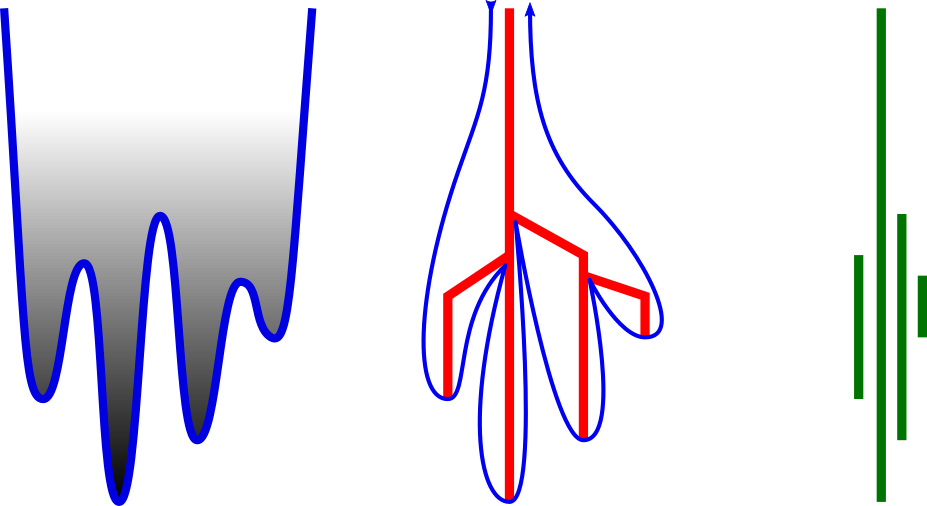
Figure 1: Graph of a function (left), its merge tree and the corrsponding contour walk (middle) and the pile of stems (bars).

It is well known that the relation between a function and its planar merge tree is essentially bijective:

Lemma 2.2.

The height walk corresponding to the merge tree $\mathtt{T}_{f}$ is right-equivalent (i.e. equal up to a reparametrization of the argument) to $f$.

2.2.3 From $\mathbf{PH}_{0}$ to merge trees

Constructions above essentially answer the natural question about the space of univariate functions generating a particular collection of bars as its $\mathbf{PH}_{o}$ diagram. The extra data necessary to rebuild the planar merge tree (and therefore the function generating that merge tree, up to reparametrization) from a (locally finite) collection of bars, are the data a) on their parental attachments, and b) on their planar order.

This result was first published by J. Curry [Cur17]: Let $f$ be a univariant function with the longest bar $-\infty\leq b_{\infty}<d_{\infty}\leq\infty$. Assume that the number of bars straddling each interval (i.e. the $\mathbf{PH}_{0}$-content of $\mathtt{Q}(b,d)$) is finite (i.e. the function is tame).

Proposition 2.3 ( [Cur17]).

The merge tree is uniquely reconstructed by the (arbitrary) attachment relation on the stems (how each bar with exception of the longest one is attached to one of the straddling bars), and by the chiralities of the stems.

We remark that one can generalize this Proposition 2.3 to functions on higher-dimensional Euclidean spaces $\mathbb{R}^{d}$ as follows:

Theorem 2.4.

The space of Morse functions on $\mathbb{R}^{d}$ with all critical points of neighboring indices $0$ and $1$ and fixed $c$-persistence diagram and the bar attachment data is homotopy equivalent to the product of $(d-1)$-dimensional spheres, one for each bar.

The proof will appear elsewhere.

2.2.4 Chirality

A bar (i.e. a point $(b,d)$ in the persistence diagram) corresponds to two events, birth of a connected component of the sublevel set $X_{\cdot}$ at height $b$, and its death, i.e. merger of two connected components, at height $d$. Clearly, this implies that there exists a (local) minimum of $f$ with the critical value $b$ and a (local) maximum with the critical value $d$.

Definition 2.5.

We will be referring to the critical points corresponding to a par $(b,d)$ in $\mathbf{PH}_{0}$ as coupled.

Given a coupled pair of local maximum and minimum, we will refer to the right or left orientation of $0$-dimensional bar in a persistence diagram of a univariate function, when it is attached to its parent stem, as chirality. There are two possible chiralities which we will denote as $\mathbf{M}$  and $\mathbf{F}$.

Formally,

Definition 2.6.

A bar $(b,d)=(f(s),f(t))$ (here $s,t$ are the critical points corresponding to the critical values $b,d$) is an $\mathbf{M}$  if the local maximum follows local minimum, i.e. if $s<t$, and an $\mathbf{F}$  otherwise, - i.e. if $s>t$.

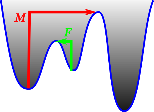
Figure 2: Coupled critical points: $\mathbf{M}$(in red) and $\mathbf{F}$(in green).

Remark 2.7.

Chiralities might be a useful tool to capture potential asymmetry of a time series with respect to the time reversal, a prominent topic in econometric literature. In [LNR⁺12], an approach somewhat resembling our chiralities was proposed.

In Section 5 we will compute average excess of $\mathbf{F}$  over $\mathbf{M}$  in Brownian trajectories with drift.

3 Bars and Automata

In this section we will set up necessary apparatus to analyze bar decomposition of a univariate function. Our key observation is that bars in a persistence diagram for a function on the real line are in direct correspondence with the windings of the function around an interval.

In what follows we will be working primarily with the functions on an interval which tend to their global minimum on the left end, and to their global maximum on the right. One can always relate this particular version with other settings (say, where the function tends to its global supremum on both ends), by adding a monotonic function interpolating global maximum and minimum at one of the interval ends: such a transformation changes the persistence diagram in an obvious way.

3.1 Winding of a function around an interval

Recall that we say that a point $(b,d),b<d$ in the persistence diagram (or the corresponding bar $[b,d]$) straddles the interval $[b^{\prime},d^{\prime}]$ if $b\leq b^{\prime}<d^{\prime}\leq d$.

Given an interval $[b,d]$, and a continuous function $f$ on $(t_{0},t_{1})=I\subset\mathbb{R}$, starting below $b$ and ending above $d$ on $I$ (i.e. $\limsup_{t\to t_{0}}f<b<d<\liminf_{t\to t_{1}}f$), one can define sequences of alternating $b$- and $d$-times $t_{0}^{b}<t_{1}^{d}<\ldots<t_{k}^{d}<t_{k}^{b}<\ldots$ by setting, iteratively,

$$t_{0}^{b}=t_{0};\mathrm{\ for\ }k\geq 1,t^{d}_{k}=\min\{t:f(t)=d,t\in I,t>t^{b}_{k-1}\},t^{b}_{k}=\min\{t:f(t)=b,t\in I,t>t^{d}_{k}\}.$$ (1)

(We set the minimum over an empty subset of $I$ to be $t_{1}$).

This sequence is obviously finite, if the interval $I$ is bounded.

Definition 3.1.

A winding of $f$ around the interval $[b,d]$ is a pair $\{t_{k}^{b},t_{k}^{d},k\geq 1\}$ in the sequence thus generated.

(See Fig. 3, right display, for an example of a function with two windings around an interval.) We remark, that the continuity of $f$ implies that the set of windings in any compact subset of $I$ is finite.

One has the following

Lemma 3.2.

The number of the bars in $\mathbf{PH}_{0}(f)$ straddling the interval $[b,d]$, or, equivalently, the $\mathbf{PH}_{0}$ content of the quadrant $\mathtt{Q}(b,d)$, is equal to the number of windings of $f$ around $[b,d]$, plus one.

Proof.

On one hand, to each winding $(t^{b}_{k},t^{d}_{k})$ one can associate the unique connected component of $I_{b}:=\{f\leq b\}$ having $t_{k}^{b}>t_{0}$ as its left end. On the other hand, to any component of $[t_{-},t_{+}]\subset I_{b}$ outside the one having $t_{0}$ in its closure, one can associate the winding with the left end $t_{-}$. This is manifestly a bijection between the windings and all but the leftmost components of $I_{b}$. ∎

This definition of windings is identical to the well-known construction of "upcrossings" used in the standard proof of Doob’s martingale convergence theorem.

3.2 Finite automata

To study windings of a function around an interval, or more generally, the interactions of the function with one or more intervals, it is convenient to encode them with a scheme using finite automata.

3.2.1 States, levels, transitions

The finite automata we will be dealing with will have states $s\in S$ with real numbers $r_{s},s\in S$, the states’ levels, assigned.

Each state will have at most two potential transitions. Special absorbing states $\omega_{\cdot}$ have no outgoing transitions; a unique starting state $\alpha$ has no state transitioning into it. Each non-absorbing state has two potential transitions and is a target of at least one transition.

Of two transitions possible from a non-absorbing state $s$, one leads to a state with a higher level; one to a state with a lower level.

The shortest interval containing the labels of all of the finite states is called the span of the automaton.

3.2.2 Symbolic trajectories

Fix a finite automaton described in 3.2.1 with the span $(b_{*},d_{*})$.

Consider a continuous function $f$ on an interval $I=(t_{0},t_{1})$ crossing the span of the automaton: such a function starts below the span of the automaton, and ends above it (i.e. $f(t_{0})+<b_{*};f(t_{1}-)>d_{*}$). Each function crossing the span defines a finite symbolic trajectory: a sequence of states and transitions between them. Transition to one state to another happens when the function, after taking the value at the level of the former state, first hits the level of the latter state.

Namely, assume that the finite automaton is in a state $s$ at instant $t$: $f(t)=r_{s}$. If there are two outgoing transitions out of $s$ leading to the states $s_{+}$ and $s_{-}$, with $r_{s_{+}}>r_{s}>r_{s_{-}}$, then the next state is whichever level, $r_{s_{+}}$ or $r_{s_{-}}$ the function $f$ reaches first. If there is just one transition from $s$, (leading to a state with a higher level), the automaton transitions there as soon as the function hits that level after the time $t$.

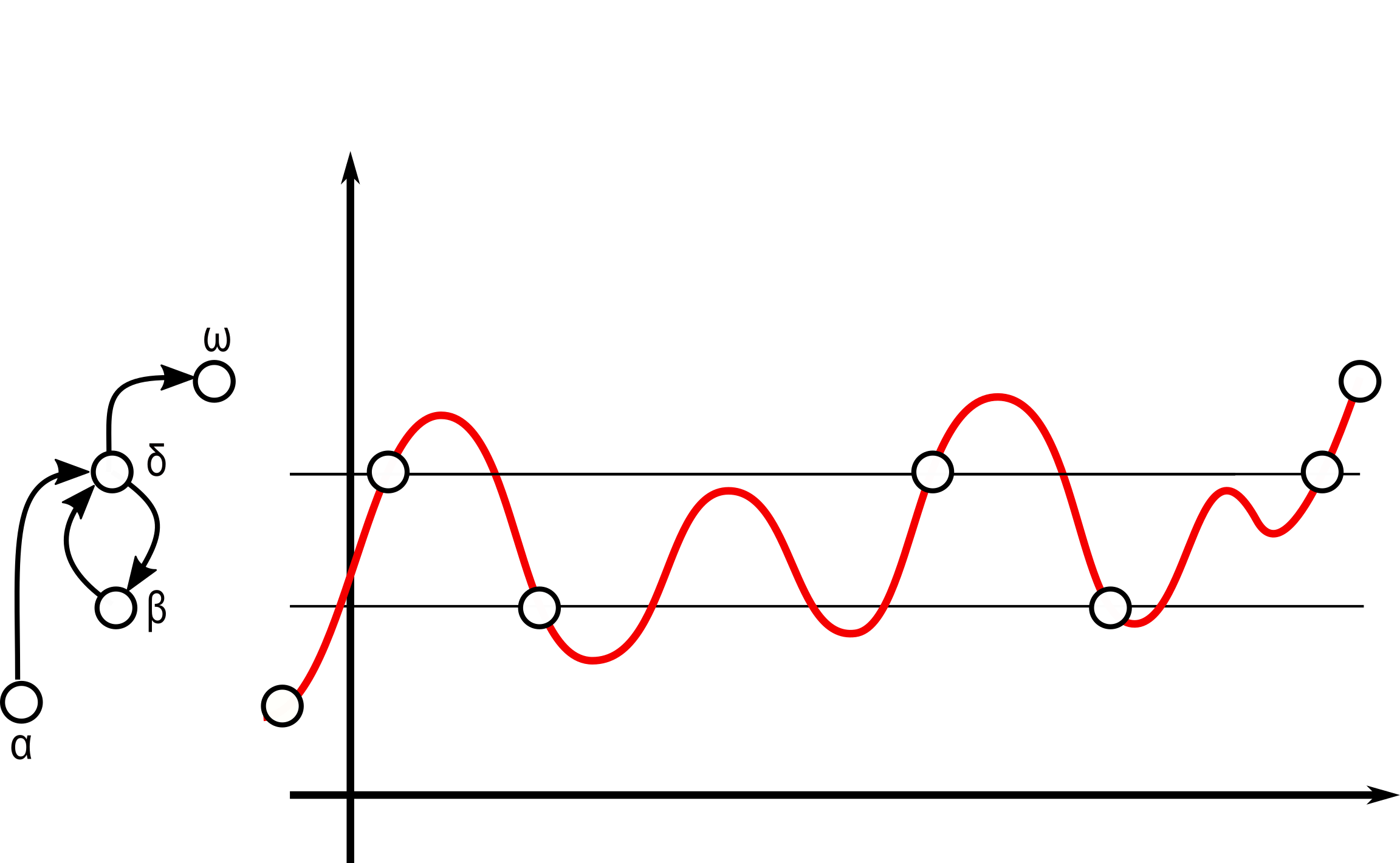
Figure 3: The finite automaton counting windings of a function around an interval. The symbolic trajectory corresponding to the function shown above is $\alpha\to\delta\to\beta\to\delta\to\beta\to\delta\to\omega$. There are two transitions $\delta\to\beta$, and two windings around the interval $[b,d]$.

The resulting sequence of states and arrows is called symbolic trajectory corresponding to the function $f$.

The following is immediate:

Lemma 3.3.

The symbolic trajectory of a continuous function crossing the span of a finite automaton is finite.

∎

3.2.3 Automata and windings around an interval

The simplest useful finite automaton of this kind described above is (shown on he left display of Fig. 3) has a starting state $\alpha$ at level $a$; two finite states $\beta$ and $\delta$ with levels $b$ and $d$, and an absorbing state $\omega$ with level $o$; with assumption $a<b<d<o$. The transitions are $\alpha\to\delta$, $\delta\to\beta,\delta\to\omega$, and $\beta\to\delta$.

Again, the following is immediate:

Proposition 3.4.

For a continuous function $f$ crossing the span of this automaton, the number of $\delta\to\beta$ transitions in the corresponding symbolic trajectory is one less than to the number of bars straddling the interval $(b,d)$ in the persistence diagram $\mathbf{PH}_{0}$ of $f$.

∎

(Remark: The one extra bar is the "infinite" one, spanning the $\inf f$ and $\sup f$.)

3.2.4 Other uses of symbolic trajectories

As a general remark, the automata introduced in Section 3.2 seem to be relevant in numerous practical situations, e.g. in financial "technical analysis", an area of financial investment lore, where the patterns of a stock or index performance are used to predict its future evolution (see, e.g. [LMW00]). Among other problems with this approach one cites often the vague, informal way the patterns are define. One might argue that using the automata formalism introduced here one can define at least some of the patters rigorously, and pursue more formal analysis of their predictive properties (see Appendix C).

4 Persistence Diagram for Brownian Walks

Our focus in this note on the properties of persistent diagrams for Brownian motions, the simplest Markov processes with continuous trajectories.

Specifically, we consider Brownian motion with a drift, that is

$$f(t)=\mathbf{B}_{o}(t)+mt,$$ (2)

where $\mathbf{B}$ is the standard Brownian motion starting at $0$, on the ray $(0,\infty)$. In this and following sections we will be concerned with the persistence diagrams of a typical trajectory.

4.1 Persistence Diagrams as Point Processes

Almost surely, there is unique bar $(b_{\infty},d_{\infty})=(\inf_{t>0}f(t),\infty)$.

Other bars are finite, forming to a random persistence diagram $\mathbf{PH}_{0}$. Our interpretation of this persistence diagram is to view it as a point process, a random measure consisting of sum of $\delta_{(b,d)}$ over all bars $(b,d)$.

Tameness of the this point process, that is the fact that the content of any NW-quadrant with its apex above the diagonal is almost surely finite, follows, again, from the mentioned above general results in [BW16]) that the persistence diagram of any Hölder function is tame, and well-known fact that the trajectory of the Brownian motion (with any smooth drift) is almost surely $1/2$-Hölder.

4.1.1 Process decomposition

Following the definitions of Section 3.2.2, we consider symbolic trajectories corresponding to (continuous) trajectories of our Brownian motions. To fit the definitions, we will assume from now on that the span of the finite automaton used to define the symbolic trajectory is contained in the positive half-line. Under this assumption, the trajectories of the Brownian motion with drift cross the span a.s., resulting in (random) symbolic trajectories.

The times of transitions between the states of such symbolic trajectories are, clearly, stopping times with respect to the filtration $\{\mathcal{F}_{\tau}\}_{\tau\geq 0}$ generated by the Brownian motion, and the sequence of states forms a Markov chain, as follows immediately from the strong Markov property for $\mathbf{B}^{m}$’s.

We will rely heavily on the standard fact that for any stopping time $\tau$, the process $\mathbf{B}^{m}_{t-\tau}-\mathbf{B}^{m}(\tau)$ is independent of $\mathcal{F}_{\tau}$.

4.1.2 Bars of Brownian motion with drift

As a corollary of Proposition 3.4 we obtain

Proposition 4.1.

Consider standard Brownian motion with constant drift $m>0$. Then total number of bars in $\mathbf{PH}_{0}$-persistence diagram straddling an interval $[b,d],b>0$ (or, equivalently, the $\mathbf{PH}_{0}$-content of the quadrant $Q(b,d)=\{(x,y):x<b<d<y\}$) is geometrically distributed with parameter $p=p_{m}(\Delta)=1-\exp(-2m\Delta)$, where $\Delta=d-b$.

Proof.

Indeed, the total number of windings around $[x,y]$ is the total number of times the transition $\delta\to\beta$ in the symbolic trajectory is made. The probability that the trajectory of the standard Brownian motion with drift $m$ starting at $y$ reaches $x$ before escaping to infinity (i.e. the state $\omega$) is $\exp(-2m(y-x))$. Strong Markov property implies that the the escapes to infinity after each hitting of $y$ are independent, proving the conclusion. ∎

4.1.3 Invariance properties

Let us state explicitly two invariances.

First, by standard rescaling properties, and the invariance (under the reparameterization of the argument) of the persistence diagrams imply that the same result - and all following results on the distributional properties of the persistence diagrams and chiralities, - are valid for Brownian motion with quadratic variation $\sigma^{2}$ and drift $m\sigma^{2}$. Hence we will restrict our attention to the standard Brownian motions.

Further, the distribution of the $\mathbf{PH}_{0}$ content depends only on the length of the bar $[b,d]$. This is again an immediate property of the Markov property of the process, and is valid for the laws of symbolic trajectories for any finite automaton as long as its span is within the positive half-line:

Proposition 4.2.

The distribution of a finite automaton with span in the positive half line remains the same upon simultaneous shift of all state levels by the same constant, as long as the condition on the span of the automaton are satisfied.

Proof.

Indeed, shifting the levels of all states by a positive amount $a$ would be reset to the original automaton if one restarts the process when it reaches $a$. ∎

4.1.4 Intensity measure for $\mathbf{PH}_{0}$ for Brownian motion with drift

Corollary 4.1 immediately leads to an explicit expression for the intensity measure $\mathbb{E}\mathbf{PH}_{0}$ for the point process of zero-dimensional persistence from standard Brownian motion with drift:

Proposition 4.3.

The intensity measure of $\mathbf{PH}_{o}$ is supported by the halfplane above diagonal $b<d$, and is given by the density

$$\bm{\mu}_{0}=\frac{4m^{2}e^{2m\Delta}(1+e^{2m\Delta})}{(e^{2m\Delta}-1)^{3}},$$

where $\Delta=d-b$.

In particular, near the diagonal the density explodes as $1/m(d-b)^{3}$.

Proof.

By 4.1, the expected $\mathbf{PH}_{0}$ content of the quadrants $Q_{b,d}$ is

$$q_{b,d}:=\mathbb{E}\mathbf{PH}_{0}(Q_{b,d})=p_{m}(\Delta)/q_{m}(\Delta)=\frac{1}{e^{2m\Delta}-1}.$$

The density of the intensity measure is, clearly, given by

$$\bm{\mu}_{0}(b,d)=-\frac{\partial^{2}q_{b,d}}{\partial b\partial d},$$

which gives the stated result. ∎

In particular, the density grows as $(m\Delta)^{-3}$ as $\Delta\to 0$.

5 Chiralities in Brownian trajectories

Fix an interval $\mathtt{B}=[b,d]$. Corollary 4.1 describes the distribution of the total number of the bars $\mathbf{PH}_{0}(Q(b,d))$ of the Brownian motion with drift $\mathbf{B}^{m}$ straddling $\mathtt{B}$. In this section, we address the question: how many of them will be $\mathbf{M}$, and how many $\mathbf{F}$?

5.1 Deconstructing into the bars

For a trajectory with at least $k$ straddling intervals there are $k$ pairs of times, $t_{0}^{b}<t^{d}_{1}<t^{b}_{1}<\ldots<t^{d}_{k}<t^{b}_{k}<t^{d}_{k+1}$, when the corresponding symbolic trajectory reaches the $\delta$ and $\beta$ states, in turn.

5.1.1 Splitting the trajectory

We chop the trajectory $\mathbf{B}^{m}$ that straddles the interval $I$ into $2k$ pieces, $f^{\downarrow}_{l},f^{\uparrow}_{l},1\leq l\leq k$ by setting

$$f^{\downarrow}_{l}(t):=\mathbf{B}^{m}(t^{d}_{l}+t),0\leq t\leq t^{b}_{l}-t^{d}_{l},$$

being the fragments of the trajectory traveling from $\delta$ to $\beta$, and

$$f^{\uparrow}_{l}(t):=\mathbf{B}^{m}(t^{b}_{l}+t),0\leq t\leq t^{d}_{l+1}-t^{b}_{l},$$

their upward counterparts.

Proposition 5.1.

Conditioned on the event that the number of bars straddling $[b,d]$ is at least $k$, the random processes $f^{\uparrow}_{l},f^{\uparrow}_{l},l=1,\ldots,k$ are independent. Moreover the processes $f^{\uparrow}_{l},l=1,\ldots,k$ are identically distributed, as well as the processes $f^{\uparrow}_{l},l=1,\ldots,k$ are.

Proof.

This follows, again, from the strong Markov property of the Brownian motion with drift.∎

We remark that the distributions of $f^{\downarrow}$ are those of the standard Brownian motion starting at $d$ and stopped once it reaches $b$, while the distributions of $f^{\uparrow}$ is that of the Brownian motion with drift $m$ started at $b$ and stopped when it reaches $d$.

The collection of the maximal values of the processes $f^{\downarrow}_{l},l=1,\ldots,k$ form the set of right ends $d_{l},l=1,\ldots,k$ of the bars straddling $I$, while the minimal values of the processes $f^{\uparrow}_{l},l=1,\ldots,k$ form the set of their left ends $b_{l},l=1,\ldots,k$.

Almost surely, these local maximal and minimal values are distinct.

5.1.2 Excursions, spans, walls

We will need a few definitions. For a point $x$ in the domain $I$ of $f$, we will call an excursion the smallest subinterval of $I$ having $x$ as its boundary point, such that $f-f(x)$ vanishes at the endpoints of the interval, does not change its sign in its interior and is not identically $0$ there. The excursion can be right or left (depending one whether the interval has the shape $[x,y]$ or $[y,x]$), and it can be valley or hill, depending on whether the values of $f$ between $x$ and $y$ are greater or less than $f(x)=f(y)$.

For any critical point $x$ that is the endpoint of an excursion, right or left, we can the other end of the excursion interval the wall of $x$.

We will call an interval a span, if the values at the endpoints of the interval are different, and the sets where the function attains its maximal and minimal value are connected and contain the endpoints (one for minimum, one for maximum).

We will refer to a function as generic if any wall of any critical point is not a critical point itself. For example, function with all critical values different is generic, but genericity is more general than that. We note that for generic functions the walls of critical points are unique.

The following lemma is immediate:

Lemma 5.2.

Let $t_{-}<t_{1}<t_{2}<t_{+}$ be four ordered times for a generic function $f$. Then the critical points $t_{1}$ and $t_{2}$ of $f$ are coupled (as defined in 2.5) if and only if $t_{-}$ is the left wall for $t_{2}$, $t_{+}$ is the right wall for $t_{1}$ and $[t_{1},t_{2}]$ is a span.

The coupling between the left and right ends of the bars depends, clearly, only on the relative ranks of the corresponding minima and maxima. We represent these two orders as two permutations (sequences of the ranks $\{1,\ldots,k\}$): $\sigma_{+}=(u_{1},\ldots,u_{k})$ and $\sigma_{-}=(l_{1},\ldots,l_{k})$.

5.2 Symmetries of the process

The Proposition 5.1 implies

Proposition 5.3.

Conditioned on the $\mathbf{PH}_{o}(Q_{a,b})=k$ the permutations $\sigma_{+}$ and $\sigma_{-}$ are independent, uniformly distributed on the symmetric group $\mathfrak{S}_{k}$.

Proof.

Both statements follow immediately from the mutual independences of $f^{\uparrow}_{l},f^{\downarrow}_{l},\ l=1,\ldots,k$. ∎

Which of the local minima and maxima $b_{\cdot},d_{\cdot}$ are coupled, depends only on the permutations $\sigma_{+},\sigma_{-}$.

For a permutation $\sigma=(s_{1},\ldots,s_{k})$ and an index $1\leq l\leq k$, we define the left and the right walls for $l$ as

$$w_{-}(l,\sigma)=\max\{m<l:s_{m}>s_{l}\},\\ w_{+}(l,\sigma)=\min\{m>l:s_{m}>s_{l}\}$$ (3)

If the former set is empty, we formally set $w_{-}(l,\sigma)=0$; if the latter one is, we wil set $w_{+}(l,\sigma)=k+1$.

Recall that a record in a permutation $\sigma=(s_{1},\ldots,s_{k})$ is the index $l$ such that $s_{l}>s_{m},m<l$; in our terms, an index is a record iff its left wall is at $0$.

Return back to the situation of a trajectory Brownian motion with drift $\mathbf{B}^{m}$ with $k$ bars straddling the interval $I$, and the corresponding permutations $\sigma_{+}=(u_{1},\ldots,u_{k})$ and $\sigma_{-}=(l_{1},\ldots,l_{k})$ of the local extremal values above and below $d$ and $b$ respectively. We augment $\sigma_{-}$ by appending $0$ on the left.

The following slightly cumbersome lemma expresses the coupling between the maxima and minima in terms of permiattions $\sigma_{-},\sigma_{+}$.

Lemma 5.4.

Let $1\leq l\leq k$, and $l_{-}=w_{-}(l,\sigma_{+}),l_{+}=w_{+}(l,\sigma_{+})$ be its left and right wall with respect to the permutation of ranks of local maxima of bars spanning $I$. Let $n_{-}=\min\{\sigma_{-}(m),l_{-}\leq m<l$ be the minimal rank among the local minima of the $\sigma_{-}$ between left wall of $l$ and $l$ (not including). Similarly, let $n_{+}=\min\{\sigma_{-}(m),l\leq m<l_{+}$ be the minimal rank of the ranks of the local minima of the $\sigma_{-}$ between $l$ (included) and its right wall. Then the local maximum in the interval $[t^{d}_{l},t^{b}_{l}]$ is coupled to the local minimum in the interval $[t^{b}_{m},t^{d}_{m+1}]$ if and only if $m$ is the position of the larger of two ranks, $n_{-},n_{+}$.

In particular, if the local index $l$ is a record in $\sigma_{+}$, it is coupled to an index on its right, that is is a $\mathbf{F}$.

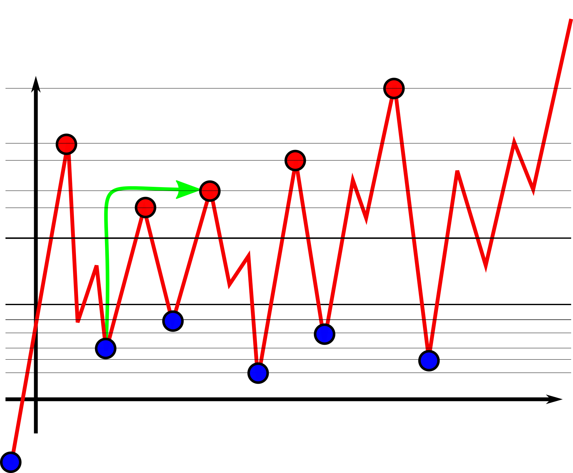
Figure 4: There $5$ bars straddling $I$ in this picture. The permutations of maxima and minima are, correspondingly, $\sigma_{+}=(41235)$ and $\sigma_{-}=(035142)$. The walls for $l=3$ are $l_{-}=1$ and $l_{+}=4$, and it is coupled with the first minimum.

Finally we can deduce the expected number of the excess of $\mathbf{F}$’s over $\mathbf{M}$’s in a Brownian motion with drift.

Theorem 5.5.

Conditioned on the number $k$ of bars straddling an interval $I$, in a trajectory of $\mathbf{B}^{m},m>0$, the expected excess of $\mathbf{F}$over $\mathbf{M}$  is equal to the expected number of records in a random $k$-permutation, that is $k$-th harmonic sum,

$$\mathbb{E}(\mathbf{F}-\mathbf{M})=H_{k}=1+1/2+\ldots+1/k.$$ (4)

Proof.

If $u_{l}$ is a record in $\sigma_{+}$, it is necessarily an $\mathbf{F}$. If it is not a record, it has proper left and right walls, $1\leq l_{-}<l<l_{+}\leq(k+1)$. Reversing the segments of $\sigma_{+}$ between $l_{-}+1$ and $l_{+}-1$, and the segment of $\sigma_{-}$ between $l_{-}$ and $l_{+}-1$ is the bijection on the pairs of permutations $(\sigma_{-},\sigma_{+})$ flipping the chirality of $l$ (and preserving the set of the records in $\sigma_{+}$). Hence, the expected excess of $\mathbf{F}$over $\mathbf{M}$  for non-record indices is zero.

Now, one can recall the standard formula on the number of records in a uniform permutation (see, e.g. [Pit06]), and the result follows. ∎

Corollary 5.6.

For Brownian motion with drift $m$ , the expected excess $\mathbb{E}(\mathbf{F}-\mathbf{M})$ in the bars straddling an interval of length $\Delta$ is

$$-\log(1-\exp(-2m\Delta)).$$

Proof.

The sum (4) gives the excess conditioned on the number of straddling bars. Summing these harmonic sums with weights $pq^{k}$, where $q=\exp(-2m\Delta)$, the probability given by Corollary 4.1, gives the desired result, after switching order of summation in the (obviously) converging series. ∎

In particular, the expected excess of $\mathbf{F}$  over $\mathbf{M}$  grows logarithmically (as $|\log(2m\Delta)|$) for small $m\Delta$; consequently the fraction of the excess among all bars straddling a short interval, disappears, as the length of the interval decreases to $0$.

6 Automata and Correlation Functions for $\mathbf{PH}_{0}$.

In this section we will construct some more complicated automata and corresponding to them Markov chains generated by symbolic trajectories of Brownian motions. These automata will be used then to derive some second-order characteristics of the $\mathbf{PH}_{0}$ point processes.

6.1 Automata and Sums over Paths

Consider a general finite state automaton, with edges marked by elements of a finitely generated monoid (or, more mundanely, by polynomials in some collection of formal variables $x_{1},x_{2},\ldots,x_{m}$), and a finite path $\bm{\pi}$ in the automaton, we define the weight $w(\bm{\pi})$ of the path to be the product of all the weights of the transitions.

If the automaton supports a Markov chain, then the weights can also incorporate the transition probabilities.

For a pair of states $\gamma,\gamma^{\prime}$ in the automaton, consider the formal power series (with nonnegative real coefficients)

$$F_{\gamma,\gamma^{\prime}}(z)=\sum_{{\gamma}\xrightarrow{\displaystyle{\bm{\pi}}}{\gamma}}w(\bm{\pi})z^{|\bm{\pi}|},$$ (5)

where the $|\bm{\pi}|$ is the length of $\pi$, and the sum is taken over all paths starting at $\gamma$ and ending at $\gamma^{\prime}$.

The usual rules – the most important being

$$F_{\gamma,\gamma"}(z)=\delta_{\gamma,\gamma"}+z\sum_{\gamma^{\prime}\to\gamma"}w({\gamma,\gamma^{\prime}})F_{\gamma^{\prime},\gamma"}(z),-$$ (6)

apply, and allow one to compute the formal power series counting the weights of families of paths in the automaton.

If the series $F_{\gamma,\gamma"}(z)$ converges at $z=1$ (perhaps, to a formal power series in other variables), omitting the argument $z$ means that we substitute $z=1$.

If the weights incorporate a Markov chain structure - as is the case n the construction of the symbolic trajectories associated by automata to Brownian motions, - one can compute the probability distributions of the numbers of times a trajectory traverses particular arrows.

6.2 Higher Windings

Let $I_{1}=[b_{1},d_{1}],I_{2}=[b_{2},d_{2}]$ are two intervals. We will be looking into the joint distribution of the numbers $b_{1},b_{2}$ of bars spanning these intervals.

Assume that the intervals are not nested, so that $b_{1}<b_{2};d_{1}<d_{2}$. In this case, the relevant automaton is shown on the Figure 5. Any continuous function that starts below $b_{1}$ and ends above $d_{2}$ generates a symbolic trajectory. The following is immediate:

Lemma 6.1.

The total number of windings around the interval $I_{1}$ is counted by the number of traversing the arrows marked with $x$ (i.e. either $\delta_{1}\to\beta_{1}$ or $\beta_{2}\to\beta_{1}$), while the number of windings around $I_{2}$ is given by the number of times the symbolic trajectory goes $\delta_{2}\to\beta_{2}$ (edge marked $y$).

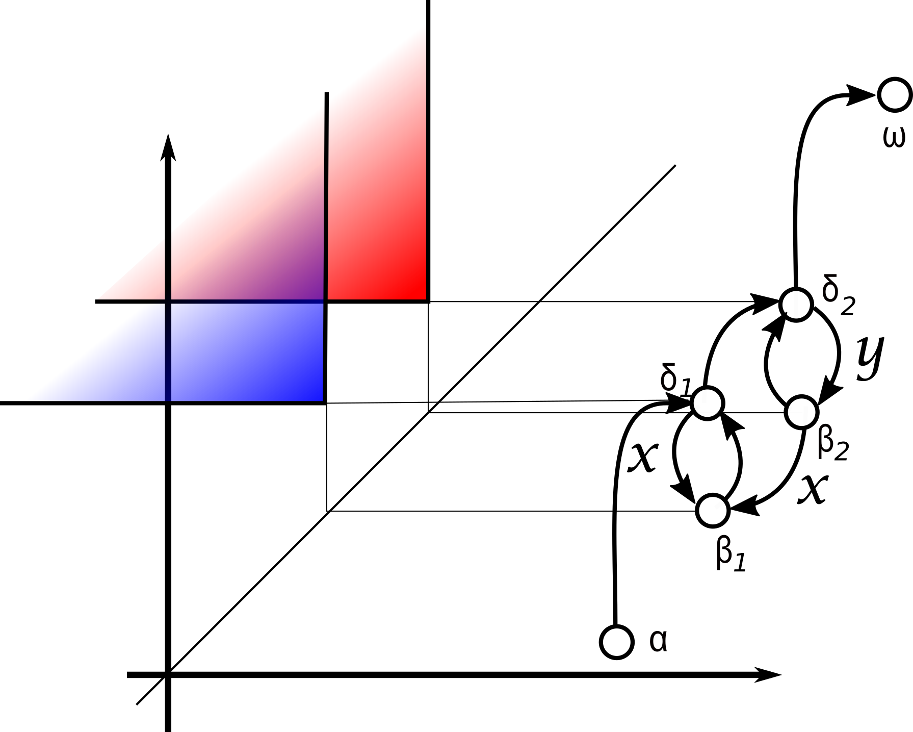
Figure 5: Windings around a pair of intervals.

If the symbolic trajectory is derived from a trajectory of Brownian motion with drift, the symbolic trajectory becomes a Markov chain. To compute its transition probabilities, we recall, that for $\mathbf{B}^{m}$ starting at $s$ exist the interval $[s-\Delta_{l},s+\Delta_{r}]$ at the right (left) end is, respectively,

$$p(\Delta_{l},\Delta_{r})=\frac{1-\mathbf{e}(\Delta_{l})}{1-\mathbf{e}(\Delta_{l}+\Delta_{r})};q(\Delta_{l},\Delta_{r})=\frac{\mathbf{e}(\Delta_{l})-\mathbf{e}(\Delta_{l}+\Delta_{r})}{1-\mathbf{e}(\Delta_{l}+\Delta_{r})}.$$ (7)

Here and in what follows, we will be using notation

$$\mathbf{e}(s)=\exp(-2ms)$$ (8)

for the character $\mathbf{e}(\cdot)$.

Using this notation, the transition probabilities in the Markov chain on the Figure 5 and the markings on the edges result in the weights given by the following table:

$$\begin{array}[]{cl}\delta_{1}\to\beta_{1}&xq_{1}=xq(d_{1}-b_{1},d_{2}-d_{1})\\ \delta_{1}\to\delta_{2}&p_{1}=p(d_{1}-b_{1},d_{2}-d_{1})\\ \beta_{2}\to\delta_{2}&p_{2}=p(b_{2}-b_{1},d_{2}-b_{2})\\ \beta_{2}\to\beta_{1}&xq_{2}=xq(b_{2}-b_{1},d_{2}-b_{2})\\ \delta_{2}\to\omega&p=p(d_{2}-b_{2},\infty)\\ \delta_{2}\to\beta_{2}&yq=yq(d_{2}-b_{2},\infty);\\ \end{array}$$ (9)

all other transitions are probability $1$.

6.3 Distributions of Windings

Using these weights, we can compute the distributions of the numbers of windings around the intervals $I_{1},I_{2}$.

Let

$$H(x,y)=F_{\alpha,\omega}(x,y)=\sum_{\alpha\xrightarrow{\displaystyle{\bm{\pi}}}\omega}w(\bm{\pi})=\sum_{{\alpha}\xrightarrow{\displaystyle{\bm{\pi}}}{\omega}}x^{k(\bm{\pi})}y^{l(\bm{\pi})}\mathbb{P}_{\bm{\pi}},$$ (10)

where $k(\bm{\pi}),l(\bm{\pi})$ are numbers of windings of the path $\bm{\pi}$ around the intervals $I_{1}$, $I_{2}$,respectively, and $\mathbb{P}(\bm{\pi})$ is the probability of the realization of the symbolic path $\bm{\pi}$, and the summation is over all paths starting in $\alpha$ and ending in $\omega$.

The formal power series (10) is, clearly, the generating function for the numbers of windings around the intervals $I_{1},I_{2}$.

To find $H(x,y)$ one uses the standard way of introducing the formal power series

$$F_{\alpha,s}(x,y)=\sum_{{\alpha}\xrightarrow{\displaystyle{\bm{\pi}}}{s}}x^{k(\bm{\pi})}y^{l(\bm{\pi})}\mathbb{P}_{\bm{\pi}},$$ (11)

for all states $s$ of the automaton, using the rules (6), and solving the resulting system of linear equations for $F_{\alpha,\cdot}$.

The work is shown in Appendix B: the final expression for the generating function $H$ is

$$H(x,y)=-\frac{(\mathbf{b}_{1}-\mathbf{d}_{1})(\mathbf{b}_{2}-\mathbf{d}_{2})}{\mathbf{d}_{1}(\mathbf{b}_{1}-\mathbf{d}_{2})+\mathbf{b}_{1}(\mathbf{d}_{2}-\mathbf{d}_{1})x+\mathbf{d}_{1}(\mathbf{b}_{2}-\mathbf{b}_{1})y+\mathbf{b}_{1}(\mathbf{d}_{1}-\mathbf{b}_{2})xy}.$$ (12)

where we denote $\mathbf{b}_{k}=\mathbf{e}(-b_{k});\mathbf{d}_{k}=\mathbf{e}(-b_{k}),k=1,2$.

6.4 Correlation density

Using equation (12), we can easily find covariance of the numbers $\mathbf{w}_{1},\mathbf{w}_{2}$ of windings around the intervals $I_{1},I_{2}$: indeed,

$$\mathtt{Cov}(I_{1},I_{2})=\left.\mathbb{E}\mathbf{w}_{1}\mathbf{w}_{2}-\mathbb{E}\mathbf{w}_{1}\mathbb{E}\mathbf{w}_{2}=\frac{\partial^{2}\log H}{\partial x\partial y}\right|_{x=y=1}.$$ (13)

Performing the calculations results in

$$\mathtt{Cov}(I_{1},I_{2})=\frac{\exp(-2m(d_{2}-b_{1}))}{(\exp(-2m(d_{1}-b_{1}))-1)(\exp(-2m(d_{2}-b_{2}))-1)}.$$ (14)

Consider the covariance (14) as a function $\mathtt{Cov}(b_{1},d_{1},b_{2},d_{2})$ of the quarterplanes with apexes at $(b_{1},d_{1})$, and $(b_{2},d_{2})$. It is clear, thanks to the bilinearity of the expectations (13), that the second moment density function is given by

$$g_{2}=\frac{\partial^{4}\mathtt{Cov}(b_{1},d_{1},b_{2},d_{2})}{\partial b_{1}\partial d_{1}\partial b_{2}\partial d_{2}}.$$ (15)

Elementary but lengthy computations yield

Theorem 6.2.

For non-nested intervals $b_{1}<b_{2};d_{1}<d_{2}$, the 2-point correlation function for the point process $\mathbf{PH}_{0}$ of 0-dimensional persistence for the standard Brownian motion with drift $m$ is given by

$$g_{2}(b_{1},d_{1};b_{2},d_{2})=\frac{64m^{4}\exp(2b_{1}+b_{2}+2d_{1}+d_{2})}{(\exp(2mb_{1})-\exp(2md_{1}))^{3}(\exp(2mb_{2})-\exp(2md_{2}))^{3}}.$$ (16)

7 Conclusion

The following problems appear natural to consider:

• It would be of interest to derive general expression for correlation functions of all orders. There are some issues related to the combinatorics of the overlapping intervals (say, computations of the Section 6 need to be modified for the nested pair of intervals $b_{1}<b_{2}<d_{2}<d_{1}$) which make this an appealing exercise.

• Similarly, the question of the distribution of the excess of $\mathbf{F}$  over $\mathbf{M}$  is of interest.

• As we mention in Appendix A, the behavior of the stack sizes in the algorithm for finding the barcodes of a time series seems nontrivial and interesting, with random updown permutation [Arn92] being the natural model for the algorithm input.

• Generalizing to higher-dimensional domains seems difficult. One might consider the results of [Pet08] as the first step to understanding persistent homology for random functions in dimension 2; but most basic questions remain open.

8 Appendices

Appendix A: Finding the Bars

Finding the bars of a time series can be done quite efficiently.

Assume that a function is given as a time series, i.e. a list of its values $f(k),k=1,\ldots,N$ at consecutive points $t_{1}<t_{2}<\ldots<t_{N}$ between which the function is assumed to be monotonic (say, linearly interpolating). Further we will assume that the function is generic.

We augment the series by setting $f(0)$ and $f(N+1)$ to respectively global minimum and maximum values: $f(0)<f(k)<f(N+1),k=1,\ldots,N$.

The output is a list with entries having the structure $(d,t_{d};b,t_{b})$, where $(d<b)$ is a bar, and $(t_{d},t_{b})$ are the locations of the corresponding (local) maxima and minima.

The algorithm maintains at all times two stacks, one with local minima, one with local maxima, ordered by critical value within each stack. Removals from the stacks happen in pairs and produce bars.

Algorithm 1 One pass bar algorithm for time series.

$\mathtt{Maxima},\mathtt{Minima}\leftarrow\mathtt{empty\ stacks}$ $\triangleright$ Initializing

$\mathtt{Direction}\leftarrow+1$ $\triangleright$ Initially, the function increases

for $t=1,\ldots,N$ do

    if $(f(t)-f(t-1))\times\mathtt{Direction}<0$ then $\triangleright$ Direction changes, so either

         if $\mathtt{Direction}=+1$ then

             $\mathtt{Maxima}.\mathtt{Push}((t-1,f(t-1))$ $\triangleright$ add the local maximum

         else

             $\mathtt{Minima}.\mathtt{Push}((t-1,f(t-1))$ $\triangleright$ …or minimum to respective stack,

         end if

         $\mathtt{Direction}=-\mathtt{Direction}$ $\triangleright$ and record change of the direction.

    else

         if $(\mathtt{Direction}=+1\&\&f(t)>\mathtt{Maxima}(0))||(\mathtt{Direction}=-1\&\&f(t)<\mathtt{Minima}(0))$ then

             $\mathtt{Output}(\mathtt{Maxima}.\mathtt{Pop},\mathtt{Minima}.\mathtt{Pop})$$\triangleright$ If hitting a wall, output a bar.

         end if

    end if

end for

Correctness of this algorithm follows immediately from Lemma 5.2 and the following observation:

Lemma 8.1.

If the interval $[t_{k},t_{l}]$ is a span, there are no critical points from the interior of the interval in the stacks.

While the time execution of the algorithm is clearly linear in the length of the time series, an interesting question arises on the depth of stacks (memory) required for its execution. In the worst case (when the local maxima are descending and the local minima ascending) the depth required is linear as well. What about the average case?

We remark that one can adapt this algorithm to register arbitrarily complicated snake-like patterns in time series.

Appendix B: Generating functions for windings around two intervals

Simplifying the notation from $F_{\alpha,s}$ to $F_{s}$, we arrive, using (6) we see that

$$b\begin{array}[]{rl}F_{\alpha}=&1\\ F_{d_{1}}=&F_{\alpha}+F_{b_{1}}\\ F_{b_{1}}=&xq(d_{1}-b_{1},d_{2}-d_{1})F_{d_{1}}+xq(b_{2}-b_{1},d_{2}-b_{2})F_{b_{2}}\\ F_{d_{2}}=&p(d_{1}-b_{1},d_{2}-d_{1})F_{d_{1}}+p(b_{2}-b_{1},d_{2}-b_{2})F_{b_{2}}\\ F_{b_{2}}=&yq(d_{2}-b_{2},\infty)F_{d_{2}}\\ F_{\omega}=&p(d_{2}-b_{2},\infty)F_{d_{2}}.\\ \end{array}$$ (17)

Here we used the notational convention (7).

Solving for $F_{\omega}$ is routine, the result is

$$H(x,y)=pp_{1}/(1-xq_{1}-yqp_{2}+xyq(q_{1}p_{2}-p_{1}q_{2}))$$ (18)

where we use shorthands

$$p=p(d_{2}-b_{2},\infty);q=q(d_{2}-b_{2},\infty);$$

$$p_{1}=p(d_{1}-b_{1},d_{2}-d_{1});q_{1}=q(d_{1}-b_{1},d_{2}-d_{1});$$

$$p_{2}=p(b_{2}-b_{1},d_{2}-b_{2});q_{2}=q(b_{2}-b_{1},d_{2}-b_{2}).$$

Using the expressions (7) for $p.,q$ we see that $H(x,y)$ is given by

$$-\frac{(\mathbf{e}(b_{1})-\mathbf{e}(d_{1}))(\mathbf{e}(b_{2})-\mathbf{e}(d_{2}))}{\mathbf{e}(d_{1})(\mathbf{e}(b_{1})-\mathbf{e}(d_{2}))+\mathbf{e}(b_{1})(\mathbf{e}(d_{2})-\mathbf{e}(d_{1}))x+\mathbf{e}(d_{1})(\mathbf{e}(b_{2})-\mathbf{e}(b_{1}))y+\mathbf{e}(b_{1})(\mathbf{e}(d_{1})-\mathbf{e}(b_{2}))xy}.$$

Appendix C: Automata and Patterns

Financial folklore often deals with patterns that can be easily translated into the language of finite automata. Without going into details here, we just illustrate encoding one of more popular pattern in "technical analysis", namely "head and shoulders" [OC95]. We suggest that most of the patterns of technical analysis can be expressed using the machinery of automata introduced in Section 3.

(Remark that – supporting the impression of very informal, folklore character of the methods of technical analysis, – while often the pattern is described, as in op.cit., as a reparametrization invariant feature, other sources, including the often cited study [LMW00], use various tools, like smoothening, that are destroying this invariance.)

The Figure 6 below shows an automaton capturing the "head and shoulders" pattern at a particular level. Each passage through the blue state indicates occurrence of the pattern.

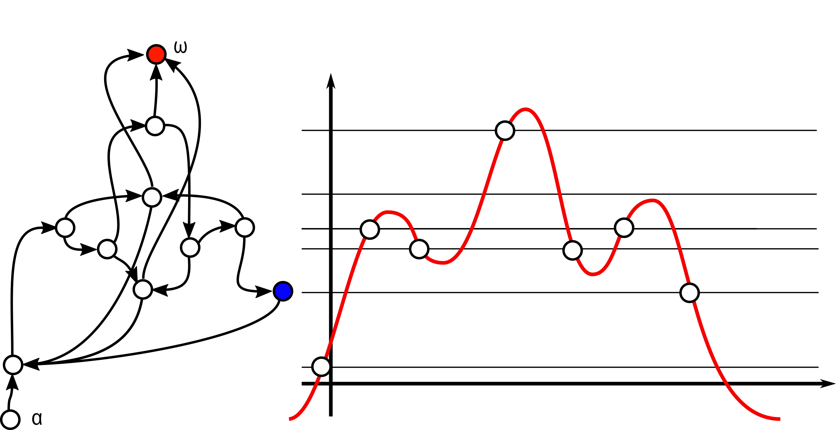
Figure 6: Finite automaton capturing the so-called "head-and-shoulder" pattern.

Rigorous, codified representation of patterns might lead to scientifically solid investigations of the actual efficiency of technical analysis and its inexplicable lure.

References

- [Arn92] Vladimir I. Arnol’d. The calculus of snakes and the combinatorics of Bernoulli, Euler and Springer numbers of Coxeter groups. Russian Mathematical Surveys, 47(1):1, 1992.
- [AT11] Robert J. Adler and Jonathan E. Taylor. Topological complexity of smooth random functions: École d’Été de Probabilités de Saint-Flour XXXIX - 2009. Number 2019 in Lecture notes in mathematics. Springer, Heidelberg ; New York, 2011. OCLC: ocn733988174.
- [BA11] Omer Bobrowski and Robert J. Adler. Distance Functions, Critical Points, and the Topology of Random Čech Complexes. arXiv:1107.4775 [math], July 2011. arXiv: 1107.4775.
- [BG18] Yuliy Baryshnikov and Robert Ghrist. Minimal Unimodal Decompositions on Trees. arXiv:1806.09673 [math, stat], June 2018. arXiv: 1806.09673.
- [BW16] Yuliy Baryshnikov and Shmuel. Weinberger. Persistence jitter. Preprint, pages 1–14, 2016.
- [Cur17] J. Curry. The Fiber of the Persistence Map. ArXiv e-prints, June 2017.
- [EH10] Herbert Edelsbrunner and John L. Harer. Computational topology. American Mathematical Society, Providence, RI, 2010. An introduction.
- [KM10] Matthew Kahle and Elizabeth Meckes. Limit theorems for Betti numbers of random simplicial complexes. arXiv:1009.4130 [math], September 2010. arXiv: 1009.4130.
- [LG05] Jean-François Le Gall. Random trees and applications. Probab. Surv., 2:245–311, 2005.
- [LMW00] Andrew W Lo, Harry Mamaysky, and Jiang Wang. Foundations of technical analysis: Computational algorithms, statistical inference, and empirical implementation. The journal of finance, 55(4):1705–1765, 2000.
- [LNR+12] Lucas Lacasa, Ángel M. Núñez, Édgar Roldán, Juan M. R. Parrondo, and Bartolo Luque. Time series irreversibility: a visibility graph approach. The European Physical Journal B, 85(6), June 2012. arXiv: 1108.1691.
- [OC95] Carol L. Osler and P. H. Kevin Chang. Head and Shoulders: Not Just a Flaky Pattern. SSRN Scholarly Paper ID 993938, Social Science Research Network, Rochester, NY, August 1995.
- [Oud15] Steve Y. Oudot. Persistence theory: from quiver representations to data analysis, volume 209 of Mathematical Surveys and Monographs. American Mathematical Society, Providence, RI, 2015.
- [Pet08] Gábor Pete. Corner percolation on $\mathbb{Z}^2$ and the square root of 17. The Annals of Probability, 36(5):1711–1747, September 2008. arXiv: math/0507457.
- [Pit06] Jim Pitman. Combinatorial Stochastic Processes: Ecole d’Eté de Probabilités de Saint-Flour XXXII - 2002. Springer, July 2006. Google-Books-ID: mW32BwAAQBAJ.