A fast Gauss transform in one dimension using sum-of-exponentials approximations

Abstract

We present a fast Gauss transform in one dimension using nearly optimal sum-of-exponentials approximations of the Gaussian kernel. For up to about ten-digit accuracy, the approximations are obtained via best rational approximations of the exponential function on the negative real axis. As compared with existing fast Gauss transforms, the algorithm is straightforward for parallelization and very simple to implement, with only twenty-four lines of code in MATLAB. The most expensive part of the algorithm is on the evaluation of complex exponentials, leading to three to six complex exponentials FLOPs per point depending on the desired precision. The performance of the algorithm is illustrated via several numerical examples.

Key words. Fast Gauss transform, sum-of-exponentials approximation, best rational approximation, model reduction.

AMS subject classifications. 31A10, 65F30, 65E05, 65Y20

1 Introduction

In this paper, we consider the evaluation of the Gauss transform in one dimension:

(1.1) $$u_{i}=\sum_{j=1}^{N}G(x_{i}-y_{j};\delta)\alpha_{j},\qquad x_{i},y_{j},\alpha_{j}\in\mathbb{R},\qquad i=1,\ldots M,$$

where the Gaussian kernel is given by the formula

(1.2) $$G(x;\delta)=e^{-\frac{x^{2}}{4\delta}}.$$

Since the Gaussian kernel is the density function of the normal distribution, the Gauss transform has broad applications in all areas of statistics such as the kernel method [13], Gaussian processes [50], nonparametric statistic models [14], density estimation [38], etc. Up to a prefactor, the Gaussian kernel is the fundamental solution of the heat equation. Thus, the Gauss transform also appears ubiquitously in integral equation methods for solving the initial/boundary value problems of the linear and semilinear heat equations that are fundamental equations for vast application areas including the diffusion process, crystal growth, dislocation dynamics, etc. See [7, 8, 11, 19, 26, 27, 28, 34, 42, 43, 52]. For fast Gauss transforms (FGTs) in higher dimensions, see [4, 20, 21, 29, 36, 39, 41, 45, 51]. These FGTs can certainly handle the one-dimensional case, but they rely on the Hermite and plane wave expansions, complex data structures and algorithmic steps, leading to nontrivial implementation task.

Here we would like to propose a simple fast algorithm based on the sum-of-exponentials (SOE) approximations of the Gaussian kernel:

(1.3) $$G(x;\delta)\approx S_{n}(x;\delta)\coloneqq\sum_{k=1}^{n}w_{k}e^{-t_{k}\frac{|x|}{\sqrt{\delta}}},$$

where $w_{k}$ and $t_{k}$ are complex weights and nodes of the SOE approximation. Very often $n$ is chosen to be an even integer and both nodes and weights appear as conjugate pairs. Thus, only half of them are needed for computing Eq. 1.1. Since the exponential function is the eigenfunction of the translation operator, the convolution with the exponential function as the kernel can be computed via a simple recurrence in linear time. This leads to an $\mathcal{O}(n(M+N))$ algorithm for computing Eq. 1.1. We would like to remark that SOE approximations have been used extensively in the design of fast algorithms. See [10, 15, 19, 27, 52].

We will show that the SOE approximation of the Gaussian kernel converges geometrically. That is, the maximum error of the approximation is $\mathcal{O}\left(c^{-n}\right)$. The optimal constant $c$ in the geometric convergence is difficult to determine. For up to about ten-digit accuracy, we use SOE approximations based on best rational approximations to $e^{x}$ on the negative real axis $\mathbb{R}^{-}=(-\infty,0]$ (see, for example, [9, 17, 49] and references therein). For about ten-digit accuracy, it only requires twelve exponentials; by symmetry, only six of them are needed in actual computation. The chief advantage of the current algorithm is that while achieving comparable performance with existing FGTs in the regime of practical interests due to the near optimality of the SOE approximations, its implementation is effortless, requiring only twenty-four lines of MATLAB code. Moreover, the algorithm is straightforward for parallelization.

The paper is organized as follows. In Section 2, we discuss several methods for obtaining SOE approximations of the Gaussian kernel. The numerical experiments of these methods are presented in Section 3. A simple fast Gauss transform in one dimension based on SOE approximations is described in Section 4. Numerical results on the 1D FGT are presented in Section 5 with further discussions in Section 6.

2 SOE approximations of the Gaussian kernel

2.1 Integral representation of the Gaussian

In [27], it is shown that the Laplace transform of the one-dimensional heat kernel $\frac{1}{\sqrt{4\pi t}}e^{-\frac{|x|^{2}}{4t}}$ is $\frac{1}{2\sqrt{s}}e^{-\sqrt{s}|x|}$. That is

(2.1) $$\frac{1}{\sqrt{4\pi t}}e^{-\frac{|x|^{2}}{4t}}=\frac{1}{2\pi i}\int_{\Gamma}e^{st}\frac{1}{2\sqrt{s}}e^{-\sqrt{s}|x|}ds.$$

Multiplying both sides by $\sqrt{4\pi t}$, replacing $t$ by $\delta$, then introducing the change of variables $s=z/\delta$, we obtain

(2.2) $$G(x;\delta)=e^{-\frac{x^{2}}{4\delta}}=\frac{1}{2\pi i}\int_{\Gamma}e^{z}\sqrt{\frac{\pi}{z}}e^{-\frac{\sqrt{z}|x|}{\sqrt{\delta}}}dz.$$

Here the branch cut of the square root function is chosen to be the negative real axis $\mathbb{R}^{-}$ and the branch is chosen to be the principal branch with $\arg(z)\in(-\pi,\pi]$. We observe that on $\mathbb{C}\setminus\mathbb{R}^{-}$ the square root function $\sqrt{z}$ always has positive real part and thus

(2.3) $$\left|e^{-\frac{\sqrt{z}|x|}{\sqrt{\delta}}}\right|\leq 1$$

for all $x\in\mathbb{R}$ and $\delta>0$. By Cauchy’s theorem, the contour $\Gamma$ in Eq. 2.2 can be any contour in the complex plane that starts from $-\infty$ in the third quadrant, around $0$, and back to $-\infty$ in the second quadrant. It is clear that the discretization of the integral in Eq. 2.2 leads to an SOE approximation Eq. 1.3 of the Gaussian kernel. In the following, we will consider integrals of the form

(2.4) $$I=\frac{1}{2\pi i}\int_{\Gamma}e^{z}f(z)dz,$$

and note that for the Gaussian kernel,

(2.5) $$f(z)=\sqrt{\frac{\pi}{z}}e^{-\frac{\sqrt{z}|x|}{\sqrt{\delta}}}.$$

2.2 Numerical evaluation of the contour integral Eq. 2.4

The numerical evaluation of the contour integral Eq. 2.4 has received much attention recently. First, the contour is parametrized via $z=z(\theta)$ with $\theta$ a real parameter, leading to

(2.6) $$I=\frac{1}{2\pi i}\int_{-\infty}^{\infty}e^{z(\theta)}f(z(\theta))z^{\prime}(\theta)d\theta.$$

The integral in Eq. 2.6 is then truncated and discretized via either the trapezoidal rule or the midpoint rule, resulting in an approximation

(2.7) $$I_{n}=\frac{h}{2\pi i}\sum_{k=1}^{n}e^{z(\theta_{k})}f(z(\theta_{k}))z^{\prime}(\theta_{k}),$$

where $\theta_{k}$ are $n$ equi-spaced points with spacing $h$. Substituting Eq. 2.5 into Eq. 2.7, we obtain an SOE approximation for the Gaussian kernel

(2.8) $$S_{n}(x;\delta)=\sum_{k=1}^{n}w_{k}e^{-t_{k}\frac{|x|}{\sqrt{\delta}}}$$

with

(2.9) $$w_{k}=\frac{h}{2\sqrt{\pi}i}\frac{z^{\prime}(\theta_{k})}{\sqrt{z(\theta_{k})}}e^{z(\theta_{k})},\qquad t_{k}=\sqrt{z(\theta_{k})}.$$

Obviously, the efficiency and accuracy of the approximation $I_{n}$ depends on the contour and its parametrization. The classical theory summarized in [40] shows that $I_{n}$ converges to $I$ subgeometrically with the rate $\mathcal{O}\left(e^{-c\sqrt{n}}\right)$. Recent developments have improved the convergence rate to geometric $\mathcal{O}\left(e^{-cn}\right)$ (see, for example, [48] for an excellent review on applications and analysis of the trapezoidal rule).

There are mainly three kinds of contours. In [44], Talbot proposed cotangent contours; simpler parabolic contours were then proposed in [33]; finally, hyperbolic contours were proposed in [31, 32]. The hyperbolic contours are applicable to a broader class of functions $f$ in Eq. 2.4 in the sense that $f$ is allowed to have singularities in a sectorial region around $\mathbb{R}^{-}$. All three contours have certain parameters that need to be optimized in order to achieve optimal convergence rate. Much research has been done on the analysis for the cotangent contours (also called Talbot contours in literature) (see, for example, [30]). The optimal choices for all three contours were first listed in [49], with detailed analysis on the optimization for parabolic and hyperbolic contours appeared in [53, 54], and the analysis on the modified Talbot contour in [12]. We remark that in [53, 54] the total number of quadrature points is $2n$ instead of $n$.

2.3 Best rational approximations to $e^{z}$ on $\mathbb{R}^{-}$

The parabolic, hyperbolic, and cotangent contours are optimized within each class. When considering the discrete approximation $I_{n}$ to $I$, we may generalize $I_{n}$ and rewrite it as follows:

(2.10) $$I_{n}=-\sum_{k=1}^{n}c_{k}f(z_{k}).$$

And the corresponding SOE approximation for the Gaussian kernel becomes

(2.11) $$S_{n}(x;\delta)=\sum_{k=1}^{n}w_{k}e^{-t_{k}\frac{|x|}{\sqrt{\delta}}},\quad w_{k}=-c_{k}\sqrt{\frac{\pi}{z_{k}}},\quad t_{k}=\sqrt{z_{k}}.$$

With a general discrete approximation in the form Eq. 2.10, it is natural to ask whether there exists a better approximation if the points $z_{k}$ can freely move in a certain region of the complex plane instead of lying on a curve and the weights $c_{k}$ are determined to minimize the quadrature error $I-I_{n}$. Obviously, this is a very difficult nonlinear global optimization problem. An interesting connection, however, is established in [49] between the approximation of $I$ by $I_{n}$ and the best rational approximation of the exponential function $e^{x}$ on $\mathbb{R}^{-}$. More precisely, it is shown there using the residue theorem and Cauchy’s theorem that

(2.12) $$I-I_{n}=\frac{1}{2\pi i}\int_{\Gamma^{\prime}}\left(e^{z}-r_{n-1,n}(z)\right)f(z)dz.$$

Here $\Gamma^{\prime}$ is a contour lying between $\mathbb{R}^{-}$ and the points $z_{k}$, and

(2.13) $$r_{n-1,n}(z)=\sum_{k=1}^{n}\frac{c_{k}}{z-z_{k}}$$

with the index $(n-1,n)$ being the type of the rational function $r$. The error formula Eq. 2.12 indicates that $I-I_{n}$ would be small if $r_{n-1,n}(z)$ is a good approximation to $e^{z}$ on $\mathbb{R}^{-}$. This is particularly true when all singularities of $f$ lie on $\mathbb{R}^{-}$ since $\Gamma^{\prime}$ can then be chosen arbitrarily close to $\mathbb{R}^{-}$, which is the case for the Gaussian kernel.

The latter problem is closely related to the famous “$1/9$” problem in rational approximation theory – the best rational approximation to $e^{z}$ on $\mathbb{R}^{-}$. The reader is referred to [49] for a review on this fascinating problem. In [17], a rigorous proof showed that

(2.14) $$\max_{z\in\mathbb{}R^{-}}\left|e^{z}-r^{\ast}_{n,n}(z)\right|=\mathcal{O}\left(9.28903\cdots^{-n}\right),$$

where $r^{\ast}_{n,n}$ is the best rational approximation of type $(n,n)$; in [9], a numerical algorithm based on the classical Remez algorithm was devised to calculate the best rational approximation $r^{\ast}_{n,n}$ and the approximation error to very high precision; in [49], an algorithm based on the Carathéodory–Fejér (CF) method was developed to compute a nearly best rational approximation of type $(n-1,n)$ for $n$ up to $14$ (see the MATLAB code cf.m in [49]).

2.4 Global reduction via balanced truncation method for SOE approximations

The type $(n-1,n)$ rational function $r_{n-1,n}$ in Eq. 2.13 is also called sum-of-poles (SOP) function. When all poles lie in, say, the left half of the complex plane, the balanced truncation method can be used to obtain an SOP approximation of smaller number of poles with a prescribed $L^{\infty}$ error. In [18], it was observed that the Laplace transform of an exponential function is a pole function, and thus the balanced truncation method can be used to reduce the number of exponentials in an SOE approximation as well. There are extensive theoretical investigations on infinite Hankel matrices [1, 2, 3, 35], and related algorithmic developments on the balanced truncation method [16], the CF method for rational approximations [22, 23, 24, 25, 46, 47], and Prony’s method for SOE approximations [5, 6]. Here we will use a simplified balanced truncation method outlined in [55] to try to further reduce the number of exponentials for a given SOE approximation of the Gaussian kernel.

3 Numerical Experiments on SOE approximations of the Gaussian kernel

We now present numerical experiments on SOE approximations of the Gaussian kernel using methods discussed in Section 2. The maximum error

(3.1) $$E_{n}=\max_{x\in\mathbb{R}}|G(x;\delta)-S_{n}(x;\delta)|$$

is estimated by setting $\delta=1$ and sampling $x$ at $0$ and $100,000$ logarithmically equally spaced points on $[10^{-5},10^{2}]$ (note that $E_{n}$ is independent of $\delta$ for any $\delta>0$).

3.1 Optimal parabolic, hyperbolic, and modified Talbot contours

Figure 3.1 shows $E_{n}$ as a function of $n$ when the contours in [49] are discretized via the midpoint rule. We observe that convergence rates are very close to theoretical values in [49] for all three contours. The maximum errors saturate at about 13-digit accuracy due to roundoff errors.

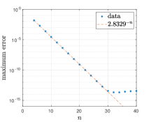
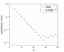
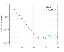
Figure 3.1: Maximum error of the SOE approximation of the Gaussian kernel as a function of $n$. Left: optimal parabolic contour. Middle: optimal hyperbolic contour. Right: optimal modified Talbot contour. See [49]. Dashed lines show the estimated convergence rate via least squares fitting of the data points.

3.2 Further reduction by the balanced truncation method

We then try to use the balanced truncation method to reduce the number of exponentials in SOE approximations. The prescribed precision for the balanced truncation method is set to $E_{n}/3$ so that the reduced SOE approximation has about the same accuracy as the original one. It turns out that SOE approximations from these three optimal contours can all be reduced. The numerical results are summarized in Figure 3.2. We observe that for all three contours, the reduced number $n_{r}$ of exponentials in the SOE approximation saturates at $18$, and the convergence rate is improved to about $\mathcal{O}\left(6.3^{-n}\right)$.

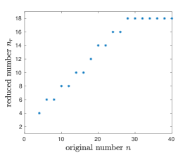
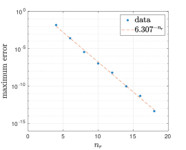
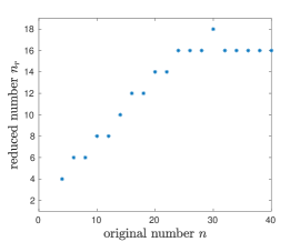
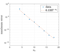
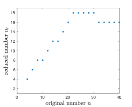
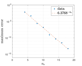
Figure 3.2: Effect of the balanced truncation method to reduce the number of exponentials in the SOE approximation of the Gaussian kernel. Left: reduced number $n_{r}$ obtained by the balanced truncated method versus original number $n$ obtained by the midpoint rule discretization of the contour integrals. Right: estimated convergence rate of the reduced SOE approximation. Top: optimal parabolic contour. Middle: optimal hyperbolic contour. Bottom: optimal modified Talbot contour.

3.3 Best rational approximations

We now turn to SOE approximations obtained by best rational approximations to the exponential function on the negative real axis. For $n\leq 14$, we use the MATLAB code cf.m in [49] to compute pole locations and weights. For $n=16$ and $18$, we have implemented the CF algorithm in cf.m in Fortran and run the code in quadruple precision to obtain pole locations and weights. The attempt of using the balanced truncation method on these SOE approximations does not lead to any further reduction. Figure 3.3 summarizes numerical results. We observe that the convergence rate is about $\mathcal{O}\left(7.5^{-n}\right)$, which is better than those obtained by optimal contours even after further reduction step by the balanced truncation method. Second, the roundoff error makes the approximation saturate at about 13-digit accuracy in double precision arithmetic. By symmetry, only half of the exponentials are needed in actual computation when $n$ is even. Hence, we only need $3$ exponentials to achieve four-digit accuracy, and $6$ exponentials to achieve about ten-digit accuracy.

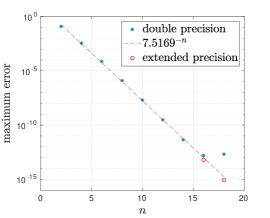
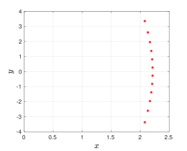
Figure 3.3: The SOE approximation of the Gaussian kernel obtained by the best rational approximation to the exponential function on the negative real axis. Left: maximum error $E_{n}$ as a function of $n$. Dashed line is the least squares fit to the first seven data points. The red circles for $n=16,18$ are calculated in extended precision. Right: locations of exponential nodes $t_{k}$ for $n=12$.

3.4 Effect of roundoff errors

We observe that all SOE approximations discussed in the previous subsections have errors saturated at about 13-digit. This is due to the ill-conditioning of the inverse Laplace transform and similar phenomena have been observed many times (see, for example, [32, 54]). Efforts have been made in stablizing the inverse Laplace transforms. In [32], a detailed analysis on the roundoff error for hyperbolic contours is presented and an additional parameter $\theta$ is introduced to balance the roundoff error with other errors (i.e., the discretization error and the truncation error). In [53], a strategy is proposed to stabilize the parabolic contours. Finally, in [12], the stabilization of the modified Talbot contours is studied.

We have tested the stabilizing techniques presented in these papers. All of them do stabilize the SOE approximations for the Gaussian kernel. However, the parabolic and Talbot contours have the approximation error saturated at about 14-digit. The accuracy of the SOE approximation using unoptimized hyperbolic contours in [32] can go down to almost machine precision in double precision arithmetic. And the balanced truncation method will reduce the number of exponentials and improve the convergence rate greatly.

In a certain sense, the ill-conditioning of the inverse Laplace transform can be viewed as an advantage when we try to construct SOE approximations for the Gaussian kernel. To be more precise, there are a wide range of parameters and contours that will lead to quite different SOE approximations with about same accuracy and the same number of exponentials. Such phenomena are already shown in Subsection 3.2. To demonstrate that the SOE approximation can achieve close to machine precision, we show one of our numerical experiments in Figure 3.4. Here we use the hyperbolic contour in [32] $z=\lambda(1-\sin(0.8+iu))$ with $a=\cosh^{-1}(2/((1-\theta)\sin(0.8)))$, $\lambda=0.6\pi(1-\theta)n/a$, the step size $h=2a/n$. The parameter $\theta$ is set to $1/4$ for $n\leq 16$ and $12/n$ otherwise. We observe that at $n_{r}=24$, the error of the reduced SOE approximation is about $2.0\times 10^{-15}$, at least ten times smaller than those by other methods that we studied.

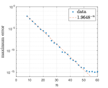
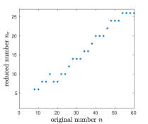
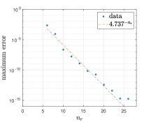
Figure 3.4: SOE approximation of the Gaussian kernel with smaller roundoff error. Left: errors of SOE approximations by a hyperbolic contour in [32]. Middle: reduction by the balanced truncation method. Right: improved convergence rate. Dashed lines show the estimated convergence rate via least squares fitting of the data points.

4 A simple fast Gauss transform in one dimension

We now present a fast algorithm for the Gauss transform in one dimension using SOE approximations. The algorithm has been known in the field of fast algorithms. Most recently it has been used in [15], where SOE approximations are developed for the kernel $\frac{1}{x}$ on $[\delta,R]$. Since the SOE approximations for the Gaussian kernel is valid in the whole real axis, the algorithm in [15] can be simplified a bit, which is discussed briefly below.

We first sort both target and source points in ascending order. In the following discussion, we will assume that targets and sources are already sorted. Substituting the SOE approximation Eq. 1.3 into Eq. 1.1 and exchange the order of summations, we obtain

(4.1) $$u_{i}\approx\sum_{k=1}^{n}w_{k}h_{k,i},\qquad i=1,\ldots,M$$

where

(4.2) $$h_{k,i}=\sum_{j=1}^{N}\alpha_{j}e^{-t_{k}\frac{|x_{i}-y_{j}|}{\sqrt{\delta}}}.$$

We further split $h_{ki}$ into two terms

(4.3) $$h_{k,i}=h_{k,i}^{+}+h_{k,i}^{-},$$

where

(4.4) $$h_{k,i}^{+}=\sum_{y_{j}\leq x_{i}}\alpha_{j}e^{-t_{k}\frac{x_{i}-y_{j}}{\sqrt{\delta}}},\qquad h_{k,i}^{-}=\sum_{y_{j}>x_{i}}\alpha_{j}e^{-t_{k}\frac{y_{j}-x_{i}}{\sqrt{\delta}}}.$$

It is clear that $h_{k,i}^{+}$ satifies the forward recurrence

(4.5) $$h_{k,i+1}^{+}=e^{-t_{k}\frac{x_{i+1}-x_{i}}{\sqrt{\delta}}}h_{k,i}+\sum_{x_{i}<y_{j}\leq x_{i+1}}\alpha_{j}e^{-t_{k}\frac{x_{i+1}-y_{j}}{\sqrt{\delta}}},$$

and $h_{k,i}^{-}$ satifies the backward recurrence

(4.6) $$h_{k,i-1}^{-}=e^{-t_{k}\frac{x_{i}-x_{i-1}}{\sqrt{\delta}}}h_{k,i}+\sum_{x_{i}\geq y_{j}>x_{i-1}}\alpha_{j}e^{-t_{k}\frac{y_{j}-x_{i-1}}{\sqrt{\delta}}}.$$

Hence, $h_{k,i}^{\pm}$ can be computed in $\mathcal{O}(N+M)$ time for each $k$ and all $i=1,\ldots,M$.

Instead of presenting the pseudocode for the whole algorithm, we show 24-line MATLAB code for the case when the target points are identical to source points in Figure 4.1. Several remarks are as follows. First, in order to save some space we have called cf.m in [49] directly in the code. Slightly better implementation may precompute and store nodes and weights of the SOE approximation. Second, due to the absence of a genuine compiler in MATLAB, we have flipped the backward pass into a forward loop for faster memory access. The code runs at about one million points per second on a laptop with Intel(R) 2.10GHz i7-4600U CPU. Finally, when the target points and source points are different, the forward pass is replaced by the code fragment in Figure 4.2. The changes to the backward pass are similar and thus omitted.

⬇

unction u=fgt1d(x,alpha,delta)

[zs,cs] = cf(12); % call cf.m in Trefethen et al. (2006)

zs = zs(1:2:12); cs = cs(1:2:12);% take only half of the exponentials

ws = -2*sqrt(pi)*cs./sqrt(zs); % SOE approximation weights

ts = sqrt(zs/delta); % SOE approximation nodes

[xs,I] = sort(x); % sort the points in ascending order

beta = alpha(I); % align the strength vector with points

e1 = exp(-ts*diff(xs)); % compute all needed complex exponentials

n2 = length(ts); nx = length(x);

hp = zeros(n2,nx);

e2 = ones(n2,1);

hp(:,1) = beta(1)*e2;

for i = 2:nx % forward pass

hp(:,i) = beta(i)*e2+e1(:,i-1).*hp(:,i-1);

end

hm = zeros(n2,nx);

e1 = fliplr(e1);

beta = fliplr(beta);

for i = 2:nx % backward pass

hm(:,i) = e1(:,i-1).*(beta(i-1)+hm(:,i-1));

end

u = real(ws.'*(hp+fliplr(hm))); % sum over all exponential modes

Iinv(I) = 1:nx;

u = u(Iinv); % reorder u by the original target order

Figure 4.1: MATLAB code for the fast Gauss transform in one dimension when the target points are identical to the source points.

⬇

x = length(x); ny = length(y);

[xs,I] = sort(x); % sort the target points

[ys,J] = sort(y); % sort the source points

beta = alpha(J); % align the strength vector with sources

e1=exp(-ts*diff(xs)); % compute needed exponentials

hp = zeros(length(ts),nx);

i = 1; j = 1;

while i <= nx && j <= ny % sweep through targets and sources

if ys(j) < xs(i) % contribution from different sources

hp(:,i) = hp(:,i)+beta(j)*exp(-ts*(xs(i)-ys(j)));

j = j+1;

elseif ys(j) == xs(i) % contribution from the identical source

hp(:,i) = hp(:,i)+beta(j);

j = j+1;

else % forward recurrence over targets

if i < nx

hp(:,i+1) = e1(:,i).*hp(:,i);

end

i = i+1;

end

end

Figure 4.2: MATLAB code fragment for the forward pass when the target points and source points are different.

5 Numerical results

We have implemented the algorithms in Section 4 in Fortran. As to the sorting, we modify the function dlasrt.f in LAPACK 3.8.0 so that it outputs the sorted array $xs$ and an integer arrary $I$ with $xs=x(I)$. The function uses Quick Sort, reverting to Insertion sort on arrays of size $\leq 20$. Thus, the average complexity of the sorting step in our implementation is $\mathcal{O}(N\log N)$. The code is compiled using gfortran 6.3.0 with -O3 option. The results shown in this section were obtained on a laptop with Intel(R) 2.10GHz i7-4600U CPU in a single core mode. In some applications, one may need to apply the Gauss transform many times with fixed locations of points but different strength vector $\alpha$. In this case, it is advantageous to pre-sort the points and precompute all needed complex exponentials and store them in a table.

We first test the case when the target points are identical to the source points. We have tested the uniform distribution (on $[0,1]$) case and Chebyshev points case. Table 5.1 shows the results for one sample run of uniform distribution case with $\delta=1$. In the table, $N$ is the total number of points in the Gauss transform. $n_{\rm e}=n/2$ is the actual number of complex exponentials needed in the computation. $t_{\rm sort}$ is the time for the sorting step. $t_{\rm pre}$ is the time for precomputing complex exponentials. $t_{\rm rem}$ is the time for the remaining calculations. $t_{\rm total}$ is the total computational time. The time is measured in seconds. And the error is the estimated maximum relative error computed at $100$ randomly selected target points. The results for Chebyshev points are similar except that the sorting step takes much less time and thus omitted. From the table, we observe that the most expensive step is computing all complex exponentials, and the sorting step already takes a significant portion in the total computational time for the numbers $N$ shown here. Indeed, if we pre-sort the points and precompute the exponentials, the code would run as fast as Quick Sort.

Table 5.1: Results of the FGT on identical target and source points with uniform distribution.

${N}$	${\,\,\,\,\,\,\,\,\,\,n_{\rm e}}$	${t_{\rm sort}}$	${t_{\rm pre}}$	${t_{\rm rem}}$	${t_{\rm total}}$	Error
$100,000$	$3$	$0.8\text{\times}{10}^{-02}$	$0.16\text{\times}{10}^{-01}$	$0.8\text{\times}{10}^{-02}$	$0.36\text{\times}{10}^{-01}$	$0.44\text{\times}{10}^{-05}$
$1,000,000$	$3$	$0.92\text{\times}{10}^{-01}$	$0.16\text{\times}{10}^{00}$	$0.68\text{\times}{10}^{-01}$	$0.34\text{\times}{10}^{00}$	$0.43\text{\times}{10}^{-05}$
$10,000,000$	$3$	$0.10\text{\times}{10}^{01}$	$0.16\text{\times}{10}^{01}$	$0.64\text{\times}{10}^{00}$	$0.38\text{\times}{10}^{01}$	$0.43\text{\times}{10}^{-05}$
$100,000$	$4$	$0.8\text{\times}{10}^{-02}$	$0.20\text{\times}{10}^{-01}$	$0.4\text{\times}{10}^{-02}$	$0.32\text{\times}{10}^{-01}$	$0.55\text{\times}{10}^{-07}$
$1,000,000$	$4$	$0.88\text{\times}{10}^{-01}$	$0.21\text{\times}{10}^{00}$	$0.80\text{\times}{10}^{-01}$	$0.40\text{\times}{10}^{00}$	$0.55\text{\times}{10}^{-07}$
$10,000,000$	$4$	$0.10\text{\times}{10}^{01}$	$0.21\text{\times}{10}^{01}$	$0.78\text{\times}{10}^{00}$	$0.44\text{\times}{10}^{01}$	$0.55\text{\times}{10}^{-07}$
$100,000$	$5$	$0.8\text{\times}{10}^{-02}$	$0.24\text{\times}{10}^{-01}$	$0.4\text{\times}{10}^{-02}$	$0.44\text{\times}{10}^{-01}$	$0.63\text{\times}{10}^{-09}$
$1,000,000$	$5$	$0.92\text{\times}{10}^{-01}$	$0.26\text{\times}{10}^{00}$	$0.96\text{\times}{10}^{-01}$	$0.46\text{\times}{10}^{00}$	$0.62\text{\times}{10}^{-09}$
$10,000,000$	$5$	$0.10\text{\times}{10}^{01}$	$0.25\text{\times}{10}^{01}$	$0.94\text{\times}{10}^{00}$	$0.51\text{\times}{10}^{01}$	$0.56\text{\times}{10}^{-09}$
$100,000$	$6$	$0.8\text{\times}{10}^{-02}$	$0.32\text{\times}{10}^{-01}$	$0.8\text{\times}{10}^{-02}$	$0.48\text{\times}{10}^{-01}$	$0.76\text{\times}{10}^{-11}$
$1,000,000$	$6$	$0.88\text{\times}{10}^{-01}$	$0.30\text{\times}{10}^{00}$	$0.12\text{\times}{10}^{00}$	$0.53\text{\times}{10}^{00}$	$0.49\text{\times}{10}^{-11}$
$10,000,000$	$6$	$0.10\text{\times}{10}^{01}$	$0.31\text{\times}{10}^{01}$	$0.11\text{\times}{10}^{01}$	$0.57\text{\times}{10}^{01}$	$0.95\text{\times}{10}^{-10}$

The throughput is shown in Figure 5.1, where each data point is obtained by averaging $10$ sample runs with $N$ ranging from $10^{6}$ to $10^{7}$. We observe that the throughput of the whole algorithm ranges from $2.6$ to $1.7$ million points per second when $n_{e}$ increases from $3$ to $6$. If we pre-sort the points and precompute all complex exponentials, the throughput increases to $16$ to $9$ million points per second.

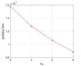
Figure 5.1: Throughput of the 1D FGT as a function of $n_{e}$ when targets are identical to sources. $n_{e}$ is half of the number of exponentials in the SOE approximation of the Gaussian kernel. Left: Throughput of the FGT without any precomputation. Right: Throughput of the FGT when points are pre-sorted and exponentials are precomputed and stored.

It is clear that the complexity of the algorithm is independent of $\delta$. Figure 5.2 shows the accuracy dependence on $\delta$ for $\delta=10^{-7},\ldots,10^{4}$. We observe that the errors slowly increases as $\delta$ increases, and saturates at the errors shown in Figure 3.3. This is because SOE approximations obtained by best rational approximations have the largest error at or near the origin, and all Gaussians will cluster around the origin as $\delta$ increases.

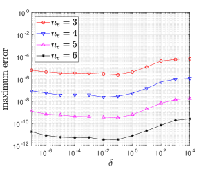
Figure 5.2: Accuracy of the FGT as a function of $\delta$.

Next we discuss the 1D FGT for the case when the target points are different from source points. The forward pass is described by the MATLAB code fragment in Figure 4.2. And the backward pass is similar. Besides calculating the exponentials $e^{-t_{k}\frac{x_{i+1}-x_{i}}{\sqrt{\delta}}}$ for march in targets, we also need to calculate the exponentials with $x_{i+1}-x_{i}$ replaced by $x_{i}-y_{j}$ or $y_{j}-x_{i}$. We tested the code for uniform distribution on $[0,1]$ and the results are shown in Table 5.2 and Figure 5.3. In Table 5.2, $t_{\rm linear}$ is the computational time excluding the sorting step. As compared to Table 5.1, the sorting time is doubled since both target and source points need to be sorted. $t_{\rm linear}$ is almost doubled since there are twice as many number of exponentials needed to be calculated. Figure 5.3 shows the throughput of the FGT, where the data points are obtained similarly as in Figure 5.1. We observe that the throughput of the full algorithm ranges from $1.5$ to $0.95$ million points per second for $n_{e}=3,\ldots,6$. We remark that the throughput of the algorithm will be close to the right panel of Figure 5.1 if we precompute and store all needed exponentials.

Table 5.2: Results of the 1D FGT on different target and source points.

${N=M}$	${\,\,\,\,\,\,\,n_{\rm e}}$	${t_{\rm sort}}$	${\,\,\,\,\,\,\,t_{\rm linear}}$	${t_{\rm total}}$	Error
$100,000$	$3$	$0.160\text{\times}{10}^{-01}$	$0.440\text{\times}{10}^{-01}$	$0.640\text{\times}{10}^{-01}$	$0.44\text{\times}{10}^{-05}$
$1,000,000$	$3$	$0.188\text{\times}{10}^{00}$	$0.432\text{\times}{10}^{00}$	$0.664\text{\times}{10}^{00}$	$0.44\text{\times}{10}^{-05}$
$10,000,000$	$3$	$0.205\text{\times}{10}^{01}$	$0.418\text{\times}{10}^{01}$	$0.675\text{\times}{10}^{01}$	$0.43\text{\times}{10}^{-05}$
$100,000$	$4$	$0.120\text{\times}{10}^{-01}$	$0.520\text{\times}{10}^{-01}$	$0.680\text{\times}{10}^{-01}$	$0.56\text{\times}{10}^{-07}$
$1,000,000$	$4$	$0.188\text{\times}{10}^{00}$	$0.556\text{\times}{10}^{00}$	$0.856\text{\times}{10}^{00}$	$0.55\text{\times}{10}^{-07}$
$10,000,000$	$4$	$0.204\text{\times}{10}^{01}$	$0.541\text{\times}{10}^{01}$	$0.800\text{\times}{10}^{01}$	$0.55\text{\times}{10}^{-07}$
$100,000$	$5$	$0.160\text{\times}{10}^{-01}$	$0.680\text{\times}{10}^{-01}$	$0.760\text{\times}{10}^{-01}$	$0.42\text{\times}{10}^{-08}$
$1,000,000$	$5$	$0.172\text{\times}{10}^{00}$	$0.672\text{\times}{10}^{00}$	$0.876\text{\times}{10}^{00}$	$0.62\text{\times}{10}^{-09}$
$10,000,000$	$5$	$0.204\text{\times}{10}^{01}$	$0.676\text{\times}{10}^{01}$	$0.918\text{\times}{10}^{01}$	$0.57\text{\times}{10}^{-09}$
$100,000$	$6$	$0.120\text{\times}{10}^{-01}$	$0.760\text{\times}{10}^{-01}$	$0.920\text{\times}{10}^{-01}$	$0.79\text{\times}{10}^{-11}$
$1,000,000$	$6$	$0.172\text{\times}{10}^{00}$	$0.792\text{\times}{10}^{00}$	$0.101\text{\times}{10}^{01}$	$0.68\text{\times}{10}^{-11}$
$10,000,000$	$6$	$0.220\text{\times}{10}^{01}$	$0.831\text{\times}{10}^{01}$	$0.110\text{\times}{10}^{02}$	$0.10\text{\times}{10}^{-09}$

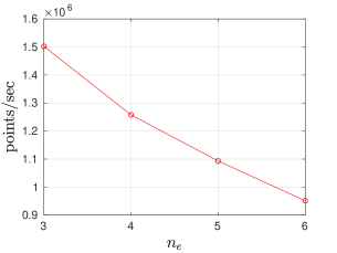
Figure 5.3: Similar to Figure 5.1, but targets and sources are different. Left: Throughput of the FGT without any precomputation. Right: Throughput of the FGT when points are pre-sorted.

6 Conclusions and further discussions

Similar to other functions discussed in [37, 49], best rational approximations to the exponential function on $\mathbb{R}^{-}$ may be used to construct nearly optimal SOE approximations for the Gaussian kernel, and a simple fast Gauss transform in one dimension has been built upon such approximations. The resulting algorithm is benign to parallelization. Indeed, the most expensive step of the algorithm is computing all needed exponentials, which is trivial to parallelize. And forward and backward passes can be easily parallelized over different modes.

The SOE approximations may also be used to speed up the FGTs in higher dimensions. Instead of standard Fourier spectral expansion, the SOE approximations can be used to diagonalize translation operators. The algorithm will be similar to the one in [10].

Another interesting fact is about the ill-conditioning of forward and backward passes. The numerical experiments in Section 3 show that the ill-conditioning of the inverse Laplace transform can be overcome and highly accurate (to almost machine precision) and efficient SOE approximations can be obtained. However, when we use such SOE approximation for the FGT, the forward and backward passes may further reduce the accuracy of the overall calculation. Indeed, the 15-digit accurate SOE approximation discussed in subsection 3.4 gives about 11-12 digit accurate solution of the Gauss transform when $N$ is one million. The SOE approximations obtained by best rational approximations do not suffer from any ill-conditioning for $n$ up to $12$, or equivalently, about ten-digit accuracy. It would be nice if one could develop accurate and efficient SOE approximations without suffering of the ill-conditioning of forward and backward passes beyond that regime.

References

- [1] V. M. Adamjan, D. Z. Arov, and M. G. Kreĭn. Infinite Hankel matrices and generalized Carathéodory-Fejér and I. Schur problems. Funkcional. Anal. i Priložen., 2(4):269–281, 1968.
- [2] V. M. Adamjan, D. Z. Arov, and M. G. Kreĭn. Infinite Hankel matrices and generalized problems of Carathéodory-Fejér and F. Riesz. Funkcional. Anal. i Priložen., 2(1):1–18, 1968.
- [3] V. M. Adamjan, D. Z. Arov, and M. G. Kreĭn. Analytic properties of the Schmidt pairs of a Hankel operator and the generalized Schur-Takagi problem. Mat. Sb. (N.S.), 86(128):34–75, 1971.
- [4] F. Andersson and G. Beylkin. The fast Gauss transform with complex parameters. J. Comput. Phys., 203(1):274–286, 2005.
- [5] G. Beylkin and L. Monzón. On approximation of functions by exponential sums. Appl. Comput. Harmon. Anal., 19(1):17–48, 2005.
- [6] G. Beylkin and L. Monzón. Approximation by exponential sums revisited. Appl. Comput. Harmon. Anal., 28(2):131–149, 2010.
- [7] K. Brattkus and D. I. Meiron. Numerical simulations of unsteady crystal growth. SIAM J. Appl. Math., 52(5):1303–1320, 1992.
- [8] R. M. Brown. The method of layer potentials for the heat equation in Lipschitz cylinders. Amer. J. Math., 111:339–379, 1989.
- [9] A. J. Carpenter, A. Ruttan, and R. S. Varga. Extended numerical computations on the “” conjecture in rational approximation theory. In Rational approximation and interpolation (Tampa, Fla., 1983), volume 1105 of Lecture Notes in Math., pages 383–411. Springer, Berlin, 1984.
- [10] H. Cheng, L. Greengard, and V. Rokhlin. A fast adaptive multipole algorithm in three dimensions. J. Comput. Phys., 155(2):468–498, 1999.
- [11] G. F. Dargush and P. K. Banerjee. Application of the boundary element method to transient heat conduction. International Journal for Numerical Methods in Engineering, 31:1231–1247, 1991.
- [12] B. Dingfelder and J. A. C. Weideman. An improved Talbot method for numerical Laplace transform inversion. Numer. Algorithms, 68(1):167–183, 2015.
- [13] A. Elgammal, R. Duraiswami, and L. S. Davis. Efficient kernel density estimation using the fast Gauss transform with applications to color modeling and tracking. IEEE Transactions on Pattern Analysis and Machine Intelligence, 25:1499–1504, 2003.
- [14] S. Geman and C.-R. Hwang. Nonparametric maximum likelihood estimation by the method of sieves. Ann. Statist., 10(2):401–414, 1982.
- [15] Z. Gimbutas, N. F. Marshall, and V. Rokhlin. A fast simple algorithm for computing the potential of charges on a line. arXiv preprint arXiv:1907.03873, 2019.
- [16] K. Glover. All optimal Hankel-norm approximations of linear multivariable systems and their -error bounds. Internat. J. Control, 39(6):1115–1193, 1984.
- [17] A. A. Gonchar and E. A. Rakhmanov. Equilibrium distributions and the rate of rational approximation of analytic functions. Math. USSR-Sb., 62(2):305–348, 1989.
- [18] L. Greengard, S. Jiang, and Y. Zhang. The anisotropic truncated kernel method for convolution with free-space Green’s functions. SIAM J. Sci. Comput., 40(6):A3733–A3754, 2018.
- [19] L. Greengard and J. Strain. A fast algorithm for the evaluation of heat potentials. Comm. on Pure and Appl. Math, 43:949–963, 1990.
- [20] L. Greengard and J. Strain. The fast Gauss transform. SIAM J. Sci. Statist. Comput., 12:79–94, 1991.
- [21] L. Greengard and X. Sun. A new version of the fast Gauss transform. Documenta Mathematica, III, pages 575–584, 1998.
- [22] M. H. Gutknecht. On complex rational approximation. II. The Carathéodory-Fejér method. In Computational aspects of complex analysis (Braunlage, 1982), volume 102 of NATO Adv. Sci. Inst. Ser. C: Math. Phys. Sci., pages 103–132. Reidel, Dordrecht-Boston, Mass., 1983.
- [23] M. H. Gutknecht. Rational Carathéodory-Fejér approximation on a disk, a circle, and an interval. J. Approx. Theory, 41(3):257–278, 1984.
- [24] M. H. Gutknecht and L. N. Trefethen. Real polynomial Chebyshev approximation by the Carathéodory-Fejér method. SIAM J. Numer. Anal., 19(2):358–371, 1982.
- [25] M. H. Gutknecht and L. N. Trefethen. Real and complex Chebyshev approximation on the unit disk and interval. Bull. Amer. Math. Soc. (N.S.), 8(3):455–458, 1983.
- [26] M. T. Ibanez and H. Power. An efficient direct bem numerical scheme for phase change problems using fourier series. Computer Methods in Applied Mechanics and Engineering, 191:2371–2402, 2002.
- [27] S. Jiang, L. Greengard, and S. Wang. Efficient sum-of-exponentials approximations for the heat kernel and their applications. Adv. Comput. Math., 41(3):529–551, 2015.
- [28] S. Jiang, M. Rachh, and Y. Xiang. An efficient high order method for dislocation climb in two dimensions. Multiscale Model. Simul., 15(1):235–253, 2017.
- [29] D. Lee, A. Gray, and A. Moore. Dual-tree fast Gauss transforms. Advances in Neural Information Processing Systems, 18:747–754, 2006.
- [30] F. F. Lin. Numerical inversion of Laplace transforms by the trapezoidal-type methods. ProQuest LLC, Ann Arbor, MI, 2004. Thesis (Ph.D.)–Oregon State University.
- [31] M. López-Fernández and C. Palencia. On the numerical inversion of the Laplace transform of certain holomorphic mappings. Appl. Numer. Math., 51(2-3):289–303, 2004.
- [32] M. López-Fernández, C. Palencia, and A. Schädle. A spectral order method for inverting sectorial Laplace transforms. SIAM J. Numer. Anal., 44(3):1332–1350, 2006.
- [33] V. L. Makarov and I. P. Gavrilyuk. Exponentially convergent parallel discretization method for the first order evolution equation. Appl. Math. Inform., 5(2):47–69, 2000.
- [34] M. Messner, M. Schanz, and J. Tausch. An efficient Galerkin boundary element method for the transient heat equation. SIAM J. Sci. Comput., 37(3):A1554–A1576, 2015.
- [35] V. V. Peller. Hankel operators and their applications. Springer Monographs in Mathematics. Springer-Verlag, New York, 2003.
- [36] R. S. Sampath, H. Sundar, and S. Veerapaneni. Parallel fast Gauss transform. in SC Proceedings of the ACM/IEEE International Conference for High Performance Computing, Networking, Storage and Analysis, New Orleans, LA, 10:1–10, 2010.
- [37] T. Schmelzer and L. N. Trefethen. Evaluating matrix functions for exponential integrators via Carathéodory-Fejér approximation and contour integrals. Electron. Trans. Numer. Anal., 29:1–18, 2007/08.
- [38] B. W. Silverman. Density estimation for statistics and data analysis. Monographs on Statistics and Applied Probability. Chapman & Hall, London, 1986.
- [39] M. Spivak, S. K. Veerapaneni, and L. Greengard. The fast generalized Gauss transform. SIAM J. Sci. Comput., 32(5):3092–3107, 2010.
- [40] F. Stenger. Numerical methods based on sinc and analytic functions, volume 20 of Springer Series in Computational Mathematics. Springer-Verlag, New York, 1993.
- [41] J. Strain. The fast Gauss transform with variable scales. SIAM J. Sci. Stat. Comput., 12:1131–1139, 1991.
- [42] J. Strain. Fast potential theory ii. layer potentials and discrete sums. J. Comput. Phys, 99:251–270, 1992.
- [43] J. Strain. Fast adaptive methods for the free-space heat equation. SIAM J. Sci. Comput., 15:185–206, 1994.
- [44] A. Talbot. The accurate numerical inversion of Laplace transforms. J. Inst. Math. Appl., 23(1):97–120, 1979.
- [45] J. Tausch and A. Weckiewicz. Multidimensional fast Gauss transforms by Chebyshev expansions. SIAM J. Sci. Comput., 31:3547–3565, 2009.
- [46] L. N. Trefethen and M. H. Gutknecht. The Carathéodory-Fejér method for real rational approximation. SIAM J. Numer. Anal., 20(2):420–436, 1983.
- [47] L. N. Trefethen and M. H. Gutknecht. Real vs. complex rational Chebyshev approximation on an interval. Trans. Amer. Math. Soc., 280(2):555–561, 1983.
- [48] L. N. Trefethen and J. A. C. Weideman. The exponentially convergent trapezoidal rule. SIAM Rev., 56(3):385–458, 2014.
- [49] L. N. Trefethen, J. A. C. Weideman, and T. Schmelzer. Talbot quadratures and rational approximations. BIT, 46(3):653–670, 2006.
- [50] J. van Waaij and H. van Zanten. Gaussian process methods for one-dimensional diffusions: optimal rates and adaptation. Electron. J. Stat., 10(1):628–645, 2016.
- [51] J. Wang and L. Greengard. An adaptive fast Gauss transform in two dimensions. SIAM J. Sci. Comput., 40(3):A1274–A1300, 2018.
- [52] S. Wang, S. Jiang, and J. Wang. Fast high-order integral equation methods for solving boundary value problems of two dimensional heat equation in complex geometry. Journal of Scientific Computing, 79(2):787–808, 2019.
- [53] J. A. C. Weideman. Improved contour integral methods for parabolic PDEs. IMA J. Numer. Anal., 30(1):334–350, 2010.
- [54] J. A. C. Weideman and L. N. Trefethen. Parabolic and hyperbolic contours for computing the Bromwich integral. Math. Comp., 76(259):1341–1356, 2007.
- [55] K. Xu and S. Jiang. A bootstrap method for sum-of-poles approximations. J. Sci. Comput., 55(1):16–39, 2013.