Photoelectron spectra after multiphoton ionization of Li atoms in the one-photon Rabi-flopping regime

Abstract

We calculate two-dimensional photoelectron momentum distributions and energy spectra after multiphoton ionization of Li atoms subject to intense laser fields in one-photon Rabi-flopping regime. The time-dependent Schrödinger equation is solved within the single-active-electron approximation using a model potential which reproduces accurately the binding energies and dipole matrix elements of the Li atom. Interaction with the external electromagnetic field is treated within the dipole approximation. We show that the Rabi oscillations of the population between the ground $2s$ state and the excited $2p$ state in the one-photon resonance regime are reflected in the energy spectra of emitted photoelectrons which manifest interference structures with minima. Transformations of the interference structures in the photoelectron energy spectra caused by the variation of the laser peak intensity and pulse duration are analyzed.

I Introduction

The phenomenon of above-threshold ionization (ATI), which was discovered about 40 years ago Agostini et al. (1979), and study of the resulting photoelectron angular distributions (PAD) attract much interest both theoretically and experimentally. Over the last four decades, this interest has grown significantly, which is related to the rapid progress of laser technology, namely, the possibility of generating extremely short and intense pulses Brabec and Krausz (2000). To get the general picture of the problem the reader can refer to a number of review papers Becker et al. (2002); Milošević et al. (2006); Agostini and DiMauro (2012).

A lithium (Li) atom, being the simplest open-shell system, presents itself a unique target for laser-atom interaction investigations, drawing both experimental Zhu et al. (2009); Schuricke et al. (2011) and theoretical Yip et al. (2010); Armstrong and Colgan (2012); Morishita and Lin (2013); Nasiri Avanaki et al. (2016); Jheng and Jiang (2017); Murakami et al. (2018) attention. From a theoretical perspective, it is important that the lithium atom has a single electron outside a closed shell, which enables the single-active-electron (SAE) model to come into play for an accurate description of the electron dynamics Schuricke et al. (2011); Morishita and Lin (2013); Jheng and Jiang (2017). For all the laser pulse parameters considered in the present paper, it is well established that the time-dependent Schrödinger equation within the SAE formulation is adequate for describing the ionization process Schuricke et al. (2011).

Photoelectron spectra and 2D momentum distributions contain various information about the ionization process, and also about the atomic or molecular internal structure. While a typical long-pulse ATI energy spectrum exhibits a well-known structure of equally-spaced peaks Agostini et al. (1979), it can also have different subtle features: Stark-induced Rydberg states resonances (Freeman resonances) Freeman et al. (1987), low energy structure (LES) Blaga et al. (2009), or interference structure originating from interfering electrons, emitted at different times Telnov and Chu (1995); Lindner et al. (2005); Wickenhauser et al. (2006); Arbó et al. (2006, 2010a, 2010b). PAD can be efficiently calculated by means of methods involving partition of the whole coordinate space into two regions and analytical propagation of the wave function in the external region without including the interaction with the atomic core Chelkowski et al. (1998); Tong et al. (2006); De Giovannini et al. (2012), with the approach based on the transition to the Kramers-Henneberger reference frame Telnov and Chu (2009), or by calculating a time-dependent flux through a spherical surface placed far enough from the atomic core Tao and Scrinzi (2012). For the processes considered in the present paper, however, the resulting photoelectrons have rather small kinetic energies (about 0.05-0.5 eV), which makes it unreasonable to neglect the Coulomb potential in the final states Chen et al. (2006); Blaga et al. (2009); Telnov and Chu (2011). For the calculation of the PAD we are providing a simulation box which is large enough to capture the dynamics of an ionized electron, which allows us to obtain the PAD directly projecting the final wave function onto the unbound states built with the scattering theory methods, including the interaction with the atomic core Wiehle et al. (2003); Chen et al. (2006).

For decades since the pioneering Rabi work Rabi (1937), population transfer between two electron states, induced by a resonant external electromagnetic field, has been a powerful tool of controlling quantum systems. In the recent paper Nasiri Avanaki et al. (2016) the high-order-harmonic generation (HHG) of a Li atom was studied in one- and two-photon Rabi-flopping regimes, revealing multipeak oscillatory pattern emerging in HHG spectra, which corresponds directly to the coherent population transfer between the ground $2s$ state and the excited $2p$, $3s$ and $3d$ states. In the present paper, we calculate photoelectron energy spectra and angular distributions of a Li atom in Rabi-flopping regime. We show that oscillations of the population of an excited state lead to the emergence of a prominent interference structure in the resulting photoelectron spectra.

The paper is organized as follows. In Sec. II we describe in detail the theoretical and computational methods applied to the present problem. The results of our calculations and all necessary theoretical analyses are presented in Sec. III. Sec. IV summarizes the results. Atomic units are used throughout the paper ($\hbar=m=e=1$), unless specified otherwise.

II Theoretical and computational methods

II.1 Electronic structure of Li atom

For the description of unperturbed electronic states of the lithium atom within SAE, we make use of the Klapisch model potential Klapisch (1971):

$$V_{\mathrm{K}}(r)=-\frac{1}{r}\left(1+\left(Z-1\right)\mathrm{e}^{-\alpha r}+Cr\mathrm{e}^{-\beta r}\right),$$ (1)

where $Z$ is the nucleus charge (for lithium, $Z=\mathrm{3}$). Other parameters are taken from Ref. Magnier et al. (1999):

$$\alpha=\text{7.90875},\;\beta=\text{3.90006},\;C=\text{10.321}.$$ (2)

The eigenvalues and eigenfunctions of the unperturbed one-electron Hamiltonian are obtained by solving the time-independent Schrödinger equation in spherical coordinates. Since the atomic core potential is spherically symmetric, the eigenfunctions take a form with separated radial and angular coordinates:

$$\psi_{nlm}(\bm{r})=R_{nl}(r)Y_{lm}(\theta,\varphi).$$ (3)

Here $Y_{lm}(\theta,\varphi)$ are the spherical harmonics with $l$ and $m$ being the angular momentum and its projection. The radial eigenfunctions $R_{nl}(r)$ are enumerated with the index $n$ for each $l$. They satisfy the following equations:

$$H_{0}^{l}R_{nl}(r)=\epsilon_{nl}R_{nl}(r),$$ (4)

$$H_{0}^{l}=-\frac{1}{2}\left[\frac{\partial^{2}}{\partial r^{2}}+\frac{1}{r}\frac{\partial}{\partial r}\right]+\frac{l(l+1)}{2r^{2}}+V_{\mathrm{K}}(r).$$ (5)

The equations are solved with the generalized pseudospectral (GPS) method (for the details, see, for example, Yao and Chu (1993); Telnov and Chu (1999); Telnov et al. (2013)). In this method, the Hamiltonian operator and wave functions are discretized on a nonuniform radial grid, and the resulting matrix eigenvalue problem for each value of $l$ is solved efficiently with the standard linear algebra routines.

For an accurate description of the resonant processes involving the initial $2s$ state and higher-lying excited states, the model must provide accurate excitation energies and dipole transition matrix elements. To make sure this is the case for the Klapisch potential, we calculate these quantities for several excited energy levels of the lithium atom. The excitation energies are listed in Table 1. As one can see, they agree very well with the experimental data from Refs. Anwar-ul Haq et al. (2005); Radziemski et al. (1995).

Table 1: Ionization and excitation energies of Li (in atomic units) calculated with the Klapisch model potential (Eq. (1)) in comparison with the experimental data from Refs. Anwar-ul Haq et al. (2005); Radziemski et al. (1995).

Transition	Model potential	Experiment
$2s\rightarrow\text{continuum}$	0.1981	0.1981
$2s\rightarrow 2p$	0.0679	0.0679
$2s\rightarrow 3s$	0.1238	0.1240
$2s\rightarrow 3p$	0.1408	0.1409
$2s\rightarrow 3d$	0.1425	0.1425

Table 2: Transition dipole matrix elements $\braket{n^{\prime}l^{\prime}}{z}{nl}$ of Li (in atomic units) calculated with the Klapisch model potential (Eq. (1)) in comparison with the matrix elements calculated by the precision linearized coupled-cluster method Safronova et al. (2012).

Transition	Model potential	Coupled-cluster method Safronova et al. (2012)
$2s\rightarrow 2p$	2.351	2.351
$2s\rightarrow 3p$	0.129	0.129
$2p\rightarrow 3s$	1.721	1.721
$2p\rightarrow 3d$	2.261	2.271

The same is also true for the corresponding transition dipole matrix elements presented in Table 2. They show excellent agreement with the matrix elements obtained by the precision linearized coupled-cluster method Safronova et al. (2012).

II.2 Time propagation of the wave function

To obtain the time-dependent wave function of the active electron $\Psi(\bm{r},t)$ in the laser field, we solve the time-dependent Schrödinger equation (TDSE):

$$i\frac{\partial\Psi(\bm{r},t)}{\partial t}=\left[H_{0}+V(\bm{r},t)\right]\Psi(\bm{r},t),$$ (6)

$$H_{0}=-\frac{1}{2}\nabla^{2}+V_{\mathrm{K}}(r),$$ (7)

for the initial $2s$ electronic state:

$$\Psi(\bm{r},0)=\psi_{2s}(\bm{r}).$$ (8)

The interaction with the external electromagnetic field is treated within the dipole approximation, which is well justified for the laser field intensities and wavelength used in the present calculations (see, for example, Ref. Ludwig et al. (2014)). In the length gauge, the interaction potential $V(\bm{r},t)$ takes the form:

$$V(\bm{r},t)=\bm{F}(t)\cdot\bm{r},$$ (9)

where $\bm{F}(t)$ is the electric field strength. We assume linear polarization of the laser field along the $z$ axis:

$$\bm{F}(t)=\bm{e}_{z}F_{0}f(t)\sin\omega t,$$ (10)

where $\omega$ and $F_{0}$ are the carrier frequency and peak field strength, respectively, while $f(t)$ is a slowly varying pulse envelope. We make use of the trapezoidal pulse shape with smooth edges to reduce the effects of varying intensity on the leading and trailing edges of the laser pulse:

$$f(t)=\begin{cases}\sin^{2}\left(\dfrac{\pi t}{2\Delta T}\right)&\mathrm{if}\quad 0\leq t\leq\Delta T,\\ 1&\mathrm{if}\quad\Delta T\leq t\leq T-\Delta T,\\ \sin^{2}\left(\dfrac{\pi(t-T)}{2\Delta T}\right)&\mathrm{if}\quad T-\Delta T\leq t\leq T,\\ 0&\mathrm{if}\quad t<0\quad\mathrm{or}\quad t>T,\end{cases}$$ (11)

where $\Delta T=0.1T$ is the switching duration, and $T$ is the pulse duration. For a pulse containing $N$ optical cycles of the frequency $\omega$, it is defined as

$$T=\frac{2\pi N}{\omega}.$$ (12)

In the present work we set the carrier wavelength to 671 nm (photon energy 0.0679 a.u.) which corresponds to a resonant one-photon transition between $2s$ and $2p$ states, and the peak intensities vary in the range from $10^{10}$ to $10^{12}$ W/cm². The laser pulse contains 20 optical cycles (duration is about 44 fs) unless specified otherwise.

To solve Eq. (6) numerically, we apply the time-dependent general pseudospectral (TDGPS) method Tong and Chu (1997) (for the details of the method, see also Telnov et al. (2013); Murakami et al. (2017)). Here we briefly outline our computational procedure. For the external field (10) linearly polarized along the $z$ axis, the projection of the electron angular momentum on this axis is conserved. Then the time-dependent wave functions can be expanded on the basis of spherical harmonics with $m=0$:

$$\Psi(\bm{r},t)=\sum_{l=0}^{l_{\mathrm{max}}}g_{l}(r,t)Y_{l0}(\theta,\varphi).$$ (13)

Here $l_{\mathrm{max}}$ is the maximum angular momentum used in the calculations. For the initial state (8), one has

$$g_{l}(r,0)=R_{20}(r)\delta_{l0}.$$ (14)

The time propagation method is based on the split-operator technique in the energy representation Tong and Chu (1997). The short-time propagator is defined by the following expression:

$$\begin{split}\Psi(\bm{r},t+\Delta t)&=\exp\left[-i\frac{\Delta t}{2}H_{0}\right]\\ &\times\exp\left[-i\Delta tV\left(t+\frac{\Delta t}{2}\right)\right]\\ &\times\exp\left[-i\frac{\Delta t}{2}H_{0}\right]\Psi(\bm{r},t),\end{split}$$ (15)

where $\Delta t$ is the time step and

$$\begin{split}\exp\left[-i\frac{\Delta t}{2}H_{0}\right]=\sum_{l=0}^{l_{\mathrm{max}}}|Y_{l0}\rangle\exp\left[-i\frac{\Delta t}{2}H_{0}^{l}\right]\langle Y_{l0}|.\end{split}$$ (16)

Eq. (15) is applied recursively starting at $t=0$ until the final wave function is obtained at $t=T$. As one can see from Eq. (16), the unperturbed propagator is actually reduced to the radial propagators corresponding to the individual angular momenta $l$, thus the angular momentum representation of the wave function (13) perfectly suits this propagation method. The unperturbed propagators $\exp\left[-i(\Delta t/2)H^{l}_{0}\right]$ are time-independent and need to be calculated only once before the propagation procedure starts. For this purpose, we use the spectral expansion:

$$\exp\left[-i\frac{\Delta t}{2}H_{0}^{l}\right]=\sum_{n}\exp\left(-i\epsilon_{nl}\frac{\Delta t}{2}\right)|R_{nl}\rangle\langle R_{nl}|.$$ (17)

Using this expansion, we can also control the contributions of extremely high energy states (large $n$), which are irrelevant for the physical processes under consideration, improving the numerical stability of the computations. The matrix dimensions of the radial propagators could be much smaller than that of the total propagator depending on the largest angular momentum $l_{\mathrm{max}}$ used. On the contrary, the external field part of the total propagator, $\exp\left[-i\Delta tV\left(t+\Delta t/2\right)\right]$, is best calculated in the coordinate ($r$ and $\theta$) representation where it appears as a multiplication operator. As any multiplication operator is diagonal in the GPS method, its calculation is not time-consuming, even though it is time-dependent and must be calculated at each time step. For the present numerical scheme to work, the wave function has to be transformed forth and back between the angular momenta $l$ and coordinate $\theta$ representations at each time step. Of course, such transformations take additional computer time but it is well compensated by the speedup due to the optimal propagator representation.

For the highest laser peak intensity 5.5 $\times 10^{11}$ W/cm² used in our calculations, the numerical parameters are as follows: the largest angular momentum is $l_{\mathrm{max}}=$ 50, the simulation box size is $R_{\mathrm{max}}=$ 400 a.u., the number of radial grid points is 311, and the number of time steps per optical cycle is 5000. For lower intensities, the parameters values may be reduced. The GPS discretization assumes zero boundary conditions for the wave function at $r=R_{\mathrm{max}}$. We do not use any special absorber at large distances to prevent spurious reflections from the box boundary. In this paper, we study the photoelectron distributions within the first ATI peak only, and the components of the wave packet corresponding to the first ATI peak (with the energies less than $0.023$ a.u.) do not reach the box boundary by the end of the laser pulse. The components with higher energies may be reflected but they are very small (the second ATI peak is 2 to 3 orders of magnitude weaker than the first one) and do not affect the dynamics of the process. Convergence of the results has been checked with respect to variation of the numerical parameters. Some calculations have also been performed using the velocity gauge of the interaction with the laser field and confirmed reliability of the corresponding length gauge results.

II.3 ATI electron spectra

At the end of the laser pulse, the transition amplitudes to various electronic states can be obtained by projecting the final wave function onto the corresponding eigenfunctions of the unperturbed Hamiltonian. We should note here that the initial wave function represents an excited ($2s$) state of the model SAE Hamiltonian, so the transitions to the ground $1s$ state are also possible. This is an obvious deficiency of the SAE model, since in the real Li atom the $1s$ state is occupied by two electrons with opposite spins, and transitions to this state are not permitted by the Pauli principle. For the laser field frequency and intensities used in the present calculations, however, the spurious transitions to the $1s$ state after the laser pulse are negligibly small. For relatively weak fields, the probabilities of multiphoton transitions depend strongly on the number of photons involved in the process. The probability of the process drops rapidly as the number of photons increases. In our case, 3 photons are required to ionize the $2s$ state while 27 photons must be emitted when a transition from the $2s$ state to the $1s$ state (unoccupied in our one-electron model) occurs. One can expect that the probability of this transition would be very small compared to the ionization probability of the $2s$ state. Our results confirm that the population of the $1s$ state remains negligibly small after the laser pulse for all the intensities used in the calculations. For the same reason, excitation and ionization probabilities of the $1s$ electronic shell in the real Li atom are also extremely small, so we can draw a conclusion that the SAE model properly describes the physical processes under consideration. The situation may change if different laser field parameters are used. Transitions between the $1s$ and other states may become noticeable for the field with the higher intensity and/or higher frequency, and this would indicate the breakdown of the present SAE model. Since fully ab initio three-electron calculations are not feasible at this time, one may think about using approximate multielectron approaches, such as a model of independent electrons moving in a mean field with the wave function described by a Slater determinant or the time-dependent density functional theory with some approximate exchange-correlation functional. However, multielectron approaches are beyond the scope of this paper because they are not really required by the physics for the laser field parameters used in the present calculations.

The photoelectron angular and energy (or momentum) distribution (PAD) can be calculated at the end of the laser pulse by projecting the wave function $\Psi(\bm{r},T)$ onto the continuum eigenfunctions $\Psi^{-}(\bm{k},\bm{r})$ of the unperturbed Hamiltonian, corresponding to the energy $E=k^{2}/2$ and asymptotic momentum direction $\hat{\bm{k}}$. The functions $\Psi^{-}(\bm{k},\bm{r})$ can be represented by the partial wave expansion Newton (1966):

$$\Psi^{-}(\bm{k},\bm{r})=\sqrt{\frac{2}{\pi}}\sum_{l=0}^{l_{\mathrm{max}}}\sum_{m=-l}^{l}i^{l}e^{-i\delta_{l}}\psi_{l}(k,r)Y^{*}_{lm}(\hat{\bm{r}})Y_{lm}(\hat{\bm{k}}),$$ (18)

where $\delta_{l}$ are the scattering phase shifts. The partial waves $\psi_{l}(k,r)$ satisfy the following equation:

$$H_{0}^{l}\psi_{l}(k,r)=\frac{k^{2}}{2}\psi_{l}(k,r)$$ (19)

and should be normalized according to the asymptotic form at $r\rightarrow\infty$:

$$\psi_{l}(k,r)\approx\frac{1}{kr}\sin\left(kr-\frac{\pi l}{2}+\frac{1}{k}\ln(2kr)+\delta_{l}\right).$$ (20)

Eq. (19) is solved by the finite-difference Numerov method (using a power series expansion of the function $\psi_{l}(k,r)$ in the vicinity of $r=0$), providing both the partial waves and phase shifts. Then the full wave function $\Psi^{-}(\bm{k},\bm{r})$ is constructed according to Eq. (18).

The differential ionization probability for the electrons emitted with the momentum $\bm{k}$ into the unit energy and solid angle intervals is calculated as

$$\frac{dP(\bm{k})}{dEd\Omega}=k|\braket{\Psi^{-}(\bm{k},\bm{r})}{\Psi(\bm{r},T)}|^{2}.$$ (21)

Photoelectron energy spectrum can be obtained by integration of PAD (21) over the angles:

$$\frac{dP(E)}{dE}=\int\frac{dP(\bm{k})}{dEd\Omega}d\Omega.$$ (22)

Then the total ionization probability can be calculated performing additional integration of the spectrum (22) over the emitted electron energy:

$$P=\int_{0}^{\infty}\frac{dP(E)}{dE}dE.$$ (23)

The same quantity can be obtained by projecting the wave function $\Psi(\bm{r},T)$ onto the eigenstates of the unperturbed discretized Hamiltonian with positive energies:

$$P=\sum_{\epsilon_{nl}>0}|\braket{\psi_{nl}(\bm{r})}{\Psi(\bm{r},T)}|^{2}.$$ (24)

Strictly speaking, the results returned by Eqs. (23) and (24) are not identical, since the wave functions (18) are not the eigenstates of the discretized unperturbed Hamiltonian. However, when the numbers of radial grid points and angular momenta are large enough to ensure convergence of the calculations, these results must be close to each other. In all our calculations the difference between the ionization probabilities obtained with Eq. (24) and Eq. (23) is less than 0.5%.

III Results and discussion

A non-resonant ionization process in the presence of an intense laser field is usually characterized in terms of the tunneling ionization (TI) and multiphoton ionization (MPI) models. The separation of these two regimes is related to the value of Keldysh parameter Keldysh (1965) $\gamma=\sqrt{I_{p}/2U_{p}}$, with $U_{p}=F_{0}^{2}/4\omega^{2}$ being the ponderomotive energy for linearly-polarized field, and $I_{p}$ being the electron ionization potential. A slowly varying strong field corresponds to $\gamma\ll 1$ and the TI model, $\gamma\gg 1$ corresponds to the MPI regime. In our present calculations, the Keldysh parameter varies from 8 to 80, which restricts us to the latter case. Photoelectron spectrum within this model contains (in the weak-field regime) equally-spaced peaks separated by a photon energy value (sharp peaks for a monochromatic external field) Agostini et al. (1979). Positions of these peaks can be roughly estimated as $E_{n}=-I_{p}+n\omega-U_{p}$, so with the increasing intensity the peaks are supposed to shift to the lower energies region.

In the present study, we set the laser wavelength to 671 nm, which matches the one-photon resonance between $2s$ and $2p$ states of the Li atom described with the Klapisch model potential (the experimental value is also 671 nm). For a description of the Rabi oscillations between the two states, we introduce the Rabi frequency and the pulse area. The Rabi frequency $\Omega$ is defined as $\Omega=F_{0}d$, where $F_{0}$ is an electric field strength, and $d$ is the transition dipole matrix element between the resonant atomic states. The pulse area $\Theta$ is defined as a product of the Rabi frequency and the full width at the half maximum (FWHM) of the laser pulse $\tau$: $\Theta=\Omega\tau$. For the trapezoidal envelope (11), $\tau=T-\Delta T$. When the pulse area reaches the value of $\pi$ (the $\pi$ pulse), the population of the initially occupied $2s$ state is completely transferred to the $2p$ state.

We present in Fig. 1 the intensity dependence of the final $2s$ and $2p$ populations as well as the total ionization probability. Rabi oscillations between the $2s$ and $2p$ states are clearly visible on the picture. Within the intensity range we used for all our calculations, the total ionization probability does not exceed 0.3. Such a choice of the intensity range guarantees no substantial ionization on the leading edge of the pulse. At higher intensities, other excited states, namely $3s$ and $3d$ states, begin to play a significant role in the ionization process. With larger ac Stark shifts Delone and Krainov (1999), resonant transitions to these states via two-photon absorption by the $2s$ electron come into play, making the ionization process more complicated.

Figure 1: Ionization probability and final population of $2s$ and $2p$ states of a Li atom exposed to linearly-polarized laser pulse. Carrier wavelength is 671 nm, which corresponds to resonance between $2s$ and $2p$ states. The pulse contains 20 optical cycles, pulse envelope is given by Eq. (11).

Photoelectron energy spectra calculated for several laser peak intensities are shown in Fig. 2. In the multiphoton ionization regime under consideration, the first ATI peak (corresponding to absorption of 3 photons) is by far dominant in the spectrum; in what follows, we will focus on the energy distribution within this peak. Here one can see a clear interference pattern that builds up in the spectrum with the increase of intensity (hence the Rabi pulse area $\Theta$) with two stable minima emerging near the energies of 0.01 and 0.005 a.u., labeled on the picture as $A$ and $B$.

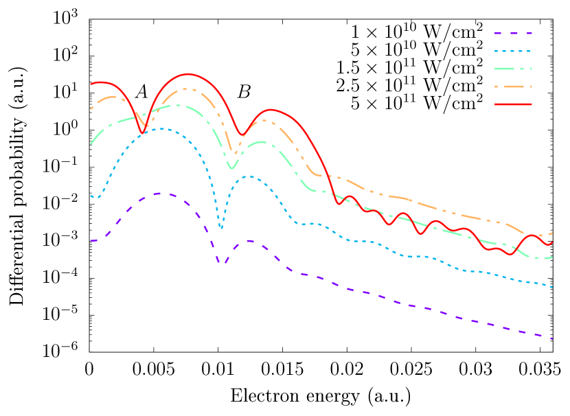
Figure 2: Photoelectron spectra of a Li atom exposed to a linearly-polarized laser pulse for different laser peak intensities. The laser wavelength is 671 nm, the pulse contains 20 optical cycles. Pulse envelope is given by Eq. (11).

To reveal the origin of these minima and obtain quantitative estimates of their positions, one can look at the time-dependent $2s$ and $2p$ populations. According to the definition of $\Theta$, the final populations of the $2s$ and $2p$ states oscillate as the peak value of the electric field and/or the pulse duration increase. In the multiphoton ionization regime ($\gamma\gg 1$), the ionization probability has a sharp dependence on the number of absorbed photons. Ionization from the $2p$ state requires absorption of $2$ photons, and we expect this ionization channel to be dominant when the $2p$ state is populated, because $3$ photons are still required to ionize the Li atom directly from the ground $2s$ state. Let us define the time-dependent populations of the unperturbed states $\psi_{nl}$:

$$P_{nl}(t)=|\braket{\psi_{nl}(\bm{r})}{\Psi(\bm{r},t)}|^{2},$$ (25)

and ionization rate as a time derivative of the instantaneous unbound-states population:

$$\Gamma(t)=\frac{d}{dt}\sum_{\epsilon_{nl}>0}P_{nl}(t).$$ (26)

We note that the quantities defined by Eqs. (25) and (26) are not observable when the external field is still on; however, they may be used to illustrate the dynamics of the excitation and ionization processes. For the laser peak intensities such as $\Theta>3\pi$ (for the trapezoidal pulse envelope (11), it corresponds to $I>2.5\times 10^{11}$ W/cm²), the rate $\Gamma(t)$ exhibits two distinct maxima corresponding to the peaks of the time-dependent $2p$-state population. Fig. 3 shows the time-dependent probabilities of some unperturbed states for the laser peak intensity $I=3\times 10^{11}$ W/cm². We also show the averaged scaled ionization rate $\Gamma(t)$. The maxima of the ionization rate are certainly correlated to the maxima of the $2p$-state population. The second (right) maximum of the ionization rate is also influenced by the right edge of the pulse envelope where the instantaneous intensity as well as ionization rate drop rapidly. The dominant ionization channel is thus controlled by the population transfer between the resonant $2s$ and $2p$ states, which “opens” and “closes” this channel with the Rabi frequency $\Omega$, even when the laser field intensity remains constant.

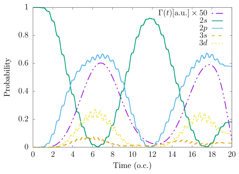
Figure 3: Scaled ionization rate $\Gamma(t)$ and the time-dependent population of the unperturbed states of a Li atom exposed to a linearly-polarized laser pulse. Laser field peak intensity is 3 $\times$ 10¹¹ W/cm², laser wavelength is 671 nm, which corresponds to resonance between $2s$ and $2p$ states. The pulse contains 20 optical cycles (o.c.), pulse envelope is given by Eq. (11).

The pattern in the ATI energy spectra (Fig. 2) can be qualitatively understood based on the lowest order of the time-dependent degenerate state perturbation theory. First, the zeroth order approximation for the wave function is obtained non-perturbatively, when the two-level system of strongly coupled resonant ($2s$ and $2p$) states is solved using the rotating wave approximation. The $2s$ and $2p$ populations oscillate with the Rabi frequency:

$$P_{2s}(t)=\cos^{2}\left(\frac{1}{2}\Omega t\right),\quad P_{2p}(t)=\sin^{2}\left(\frac{1}{2}\Omega t\right).$$ (27)

The probability amplitudes of subsequent excitation and ionization are described by the corresponding multiphoton matrix elements of the perturbation. In the multiphoton ($\gamma\gg 1$) regime, the ionization probability of the $2p$ state is much larger than that of the $2s$ state because ionization of the $2s$ state requires absorption one extra photon. For the range of the laser intensities under consideration, there are only two time moments within the pulse when the population of the $2p$ state reaches its maximum. According to Eq. (27), they are separated by the time interval equal to $2\pi/\Omega$. In the vicinities of these time moments one can see the highest ionization rate in Fig. 3. The phase difference $\Phi_{\mathrm{R}}(E)$ between the contributions to the ionization amplitude from these time moments follows from the time dependence of the multiphoton ionization amplitude:

$$\Phi_{\mathrm{R}}(E)=2\pi(E-\epsilon_{2p}-n\omega)/\Omega,$$ (28)

where $E$ is the energy of the ejected electron and $n=2$ is the number of photons absorbed. Eq. (28) predicts an interference structure in the electron energy spectra with the adjacent minima $A$ and $B$ separated by the Rabi frequency $\Omega$. We note that the interference oscillatory structure of ATI peaks can only be detected for laser pulses of finite duration; for continuous wave laser fields, the ATI energy spectrum in the resonant ionization case consists of two series of equally spaced narrow peaks shifted from each other by the Rabi frequency.

These predictions based on a simple model of Rabi oscillations in the two-level system can be checked against the results of our numerical calculations for the positions $E_{A}$ and $E_{B}$ of the minima $A$ and $B$ in the energy spectrum. Let us define two phase shifts, $\Delta\Phi_{\mathrm{R}}$ and $\Delta\Phi$:

$$\Delta\Phi_{\mathrm{R}} = 2\pi(E_{B}-E_{A})/\Omega,$$ (29)

$$\Delta\Phi = (E_{B}-E_{A})\Delta t,$$ (30)

where the time delay $\Delta t$ is obtained directly from the peak positions of the calculated time-dependent ionization rate $\Gamma(t)$: while $\Delta\Phi_{\mathrm{R}}$ makes use of the theoretically predicted time delay $2\pi/\Omega$ in the two-level system, $\Delta\Phi$ is calculated with the numerical data. Values of $\Delta\Phi$ and $\Delta\Phi_{\mathrm{R}}$, calculated for the laser intensities from $2.5\times 10^{11}$ to $5.5\times 10^{11}$ W/cm² are listed in Table 3. As one can see, the phase difference between the two adjacent minima in the energy spectra is close to $2\pi$ for both $\Delta\Phi$ and $\Delta\Phi_{\mathrm{R}}$, as expected from the interference pattern. The deviation from $2\pi$ becomes larger for $\Delta\Phi_{\mathrm{R}}$ at higher intensities. This result is well understood: the two-level system approximation becomes less accurate for higher intensities as the other higher excited electronic states begin to play a more important role in the ionization process.

The interference oscillations in Fig. 2 show up on top of the ATI peak in the energy range 0 to 0.02 a.u. where the ionization signal is the strongest and comes through the dominant ionization channel related to the resonant population transfer to the $2p$ state. As one can see, these oscillations disappear for the energies higher than 0.02 a.u. The energy range $0.02$ to $0.035$ a.u. in Fig. 2 lies already beyond the first ATI peak, and the ionization signal here is 2 to 3 orders of magnitude weaker than that at the top of the peak. Various parts of the laser pulse in the time domain (including those where the $2p$ state is not significantly populated) can make comparable contributions to the ionization signal here. Since the ionization channel responsible for the interference oscillations is not dominant in this energy range, one cannot expect to see a clear interference pattern here.

For the intensities smaller than $2.5\times 10^{11}$ W/cm², corresponding to the Rabi pulse area $\Theta<3\pi$ for the pulse containing 20 optical cycles, only one peak appears in the ionization rate, controlled by the ionization from significantly populated $2p$ state (it can also be influenced by the pulse envelope edge, see Fig. 4).

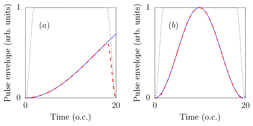
Figure 4: The laser pulse envelope (Eq. (11)) (dotted line), the Li $2p$ state population (solid line), and the schematic plot of the resulting ionization rate $\Gamma(t)$ (dashed line) for the Rabi pulse area $(a)$ $\Theta=0.6\pi$ and $(b)$ $\Theta=2\pi$. The pulse contains 20 optical cycles (o.c.).

Let us introduce the width of the peak $\delta t$ and consider the interference of the electrons ionized during this time interval. Assuming the ionization rate to be equal to some mean value $\overline{\Gamma}(E)$, the differential probability can be presented as follows:

$$\frac{dP(E)}{dE} \sim \overline{\Gamma}(E)\left|\int_{0}^{\delta t}e^{i(E-\epsilon_{2p}-2\omega)\tau}d\tau\right|^{2}$$

$$\sim\overline{\Gamma}(E)\left|\frac{\sin(E-\epsilon_{2p}-2\omega)\delta t}{(E-\epsilon_{2p}-2\omega)\delta t}\right|^{2}.$$

While $\overline{\Gamma}(E)$ corresponds only to the energy conservation, the second factor approximately describes the interference of the ionized electrons, similar to the considerations of Ref. (Arbó et al., 2010a). The minimum appearing in the spectra corresponds to the first node of this factor: with the increase of the peak width $\delta t$ (which can be done by increasing either the intensity or the pulse duration) the position of the minimum shifts to the main peak in the spectrum according to Eq. (III), which is clearly seen in the results for the small peak intensity $I=10^{10}$ W/cm² and pulses containing 13 to 20 optical cycles (see Fig. 5).

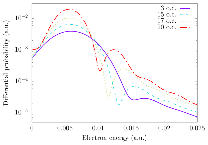
Figure 5: Photoelectron spectra of a Li atom exposed to a linearly-polarized laser pulse for various pulse duration (13-20 optical cycles (o.c.)). The laser peak intensity $I=10^{10}$ W/cm², carrier wavelength is 671 nm, pulse envelope is given by Eq. (11).

Table 3: The phase shifts $\Delta\Phi_{\mathrm{R}}$ and $\Delta\Phi$ defined by Eq. (29) and Eq. (30) respectively, calculated for different laser peak intensities.

Peak intensity, W/cm2	$\Delta\Phi_{\mathrm{R}}/2\pi$	$\Delta\Phi/2\pi$
2.5 $\times 10^{11}$	1.08	1.09
3.0 $\times 10^{11}$	0.99	1.09
3.5 $\times 10^{11}$	0.95	1.05
4.0 $\times 10^{11}$	0.91	1.04
4.5 $\times 10^{11}$	0.88	1.00
5.0 $\times 10^{11}$	0.88	1.03
5.5 $\times 10^{11}$	0.86	1.02

For the other pulse envelope functions, like Gaussian or sine-squared, the effects caused by the edges of the envelope may be more significant, leading to emergence of complex interference structures in the spectra Telnov and Chu (1995); Wickenhauser et al. (2006). However, as we have checked by performing calculations with the sine-squared pulse envelope function, the interference mechanism studied here remains dominant for this pulse shape as well, at least for relatively long pulses. Insensitivity of the Rabi-flopping interference pattern in the photoelectron spectrum to the pulse shape could facilitate its observation in the experiments.

Figure 6: Photoelectron angular and energy distribution after above-threshold ionization of a Li atom exposed to a linearly-polarized laser pulse with peak intensity $I=5\times 10^{11}$ W/cm². The pulse contains 20 optical cycles, the laser wavelength is 671 nm and corresponds to the resonance between the $2s$ and $2p$ states. The pulse envelope is given by Eq. (11). The PAD intensity scale is logarithmic and shown as a color map.

In Fig. 6, we present the PAD after multiphoton ionization of the Li atom calculated by Eq. (21) for the laser peak intensity $I=5\times 10^{11}$ W/cm². The angular distribution has a well-known ring structure. Here we show the first two rings, corresponding to the ionization by three and four photons. As known from the literature (see, e.g., Ref. Chen et al. (2006)), the number of nodes in the angular distribution equals to the dominant value of the angular momentum $l$ in the final continuum state. For the first ring in the PAD, the dominant $l=3$, as anticipated, since only three photons are required for the ionization. The radial structure of the stripes corresponds to the interference mechanism discussed above. As one can see, it is independent of the electron emission angle and reproduces the same features as the photoelectron energy spectrum.

IV Conclusion

In this paper, we have presented photoelectron angular distributions and energy spectra after multiphoton above-threshold ionization of Li atoms in the one-photon Rabi-flopping regime. The Li atom is described by the single-active-electron model with a quality core potential, which reproduces accurately the excitation and ionization energies, as well as transition dipole matrix elements. The interaction with the linearly-polarized laser field is treated in the dipole approximation using the length gauge. The time-dependent Schrödinger equation is solved efficiently with the help of the time-dependent generalized pseudospectral method. The calculations have been performed for the laser peak intensities in the range 1 $\times$ 10¹¹ to 5.5 $\times$ 10¹¹ W/cm². The carrier wavelength is set to 671 nm, so the photon energy matches the experimental transition energy between the $2s$ and $2p$ states of the Li atom.

We have shown that the population transfer between the ground $2s$ and excited $2p$ states in the resonant laser field is reflected in the photoelectron energy spectra which manifest interference oscillatory structures with the spacing between the adjacent minima equal to the Rabi frequency $\Omega$. The main ionization channel is controlled by the excited state population and switched on at specific moments in time when the ionization rate is the highest, thus implementing the double-slit interference picture in the time domain Lindner et al. (2005). The transformations of the interference structures with the increase or decrease of the pulse area have been also revealed and analyzed.

For all our calculations reported in this paper, we used the trapezoidal pulse envelope function to minimize the interference effects in the electron spectra related to the pulse shape Telnov and Chu (1995); Wickenhauser et al. (2006) and not caused by the Rabi flopping. However, we have also performed similar calculations for the sine-squared pulse envelope and found that the interference pattern due to the resonant population transfer in the Rabi-flopping regime is still dominant. We should also note that the interference structures emerging in the electron spectra in the Rabi-flopping regime are not specific to the Li atom and can be observed for the other atomic or molecular targets with similar properties of the electronic energy levels.