Stationary and dynamical properties of one-dimensional quantum droplets

Abstract

The dynamics of quantum droplets in 1D is analyzed on the basis of the variational approach (VA). It is shown that the VA based on the super-Gaussian function gives a good approximation of stationary states. The period of small oscillations of the perturbed droplet is obtained. It is found numerically that oscillations are almost undamped for many periods. Based on the VA, an existence of stable localized states for different combinations of signs of nonlinearities is demonstrated.

1 Introduction

There is a considerable progress in theoretical and experimental studies of quantum droplets (QDs) in ultracold gases [1, 2, 3, 4, 5, 6, 7, 8, 9, 10]. The existence of the quantum droplets was predicted in Ref. [1]. It is well known that a multi-dimensional Bose-Einstein condensate (BEC) with attraction between atoms experiences a collapse [11]. Quantum fluctuations can arrest the collapse in two and three dimensions. Such a possibility follows from the expression of a correction, known as the Lee-Huang-Yang (LHY) term [12], to the ground state energy of Bose gas due to quantum fluctuations. This correction corresponds to the appearance of the effective repulsion $\sim n^{5/2}$ in 3D, where $n$ is the condensate density. The balance between attraction of atoms and the effective repulsion induced by quantum fluctuations results in the possibility of the quantum droplet existence. The systems, where quantum droplets are predicted to present time, include two component BECs [1, 2, 8, 9], dipolar BECs [3], Bose-Fermi mixtures, and Bose mixtures with spin-orbit coupling [10]. Experimentally QDs are observed in dipolar BECs [3, 4] and Bose-mixtures [5, 7].

A study of quasi-one-dimensional BECs represents a particular interest [2, 8] The form of the LHY term in this case has nontrivial behavior. While in 2D and 3D LHY term describes the effective repulsion, for low densities in 1D it corresponds to the effective attraction. With an increase of the condensate density, the sign of the LHY term is changed from the attraction to the repulsion [4, 6]. Thus, there is a region where localized states in BECs with effective repulsion between atoms exist due to the effect of quantum fluctuations. A theoretical analysis of this 1D QDs was performed in recent works [2, 8].

In Ref. [2], an exact solution for 1D QDs was obtained. In experiments, an initial distribution of a BEC, formed by external traps, may not coincide with the exact solution. Therefore, it is important to develop an approach that describes the dynamics of the QD parameters in time, also in a presence of different perturbations. We mention that the variational approach (VA), based on the Gaussian trial function [8], works only for low number of atoms. The purpose of this work is to describe analytically the dynamical properties of 1D droplets using the modified variational approach, based on the super-Gaussian function. We demonstrate that such an approach gives an excellent description of the QD dynamics. Also, based on this approach we predict an existence of localized waves (solitons) for a general case of signs of quadratic and cubic nonlinearities.

The paper is organized as follows. In Section 2, the modified VA is developed. In particular, the dynamical equations for the QD parameters are derived, the parameters of stationary QDs are analyzed, and the frequency of small oscillations of the QD shape is obtained. In Section 3, an application of the VA to a general case of the system is presented. Section 4 concludes the paper.

2 The model and dynamical equations

Let us consider a two-component BEC under the action of quantum fluctuations. This system in 1D geometry is described by the following equations (c.f. Ref. [2]):

$$i\hbar\psi_{1,t}+{\hbar^{2}\over 2m}\psi_{1,xx}+(\Gamma_{s}|\psi_{1}|^{2}+\Gamma_{c}|\psi_{2}|^{2})\psi_{1}$$

$$+\Delta(|\psi_{1}|^{2}+|\psi_{2}|^{2})^{1/2}\psi_{1}=0,$$

$$i\hbar\psi_{2,t}+{\hbar^{2}\over 2m}\psi_{2,xx}+(\Gamma_{c}|\psi_{1}|^{2}+\Gamma_{s}|\psi_{2}|^{2})\psi_{2}$$

$$+\Delta(|\psi_{1}|^{2}+|\psi_{2}|^{2})^{1/2}\psi_{2}=0,$$ (1)

where $\psi_{1}$ ($\psi_{2}$) is the wave function of the first (second) component, $\Gamma_{s}=(3g+g_{c})/2$, $\Gamma_{c}=(g_{c}-g)/2$ (the self- and cross-interaction coefficients), and $\Delta=\sqrt{m}\,g^{3/2}/(\pi\hbar)$ are related to the intra- and inter-species coupling constants, $g\equiv g_{\uparrow\uparrow}=g_{\downarrow\downarrow}={2\hbar^{2}a_{s}/(ma_{\bot}^{2})}$ and $g_{c}\equiv g_{\uparrow\downarrow}$, respectively, where $g_{\uparrow\downarrow}$ is found similarly to $g_{\uparrow\uparrow}$ ($g_{\downarrow\downarrow}$) with the corresponding value of $a_{s}$. Considering the symmetric case, when $\psi_{1}=\psi_{2}=\psi_{s}\Psi$, the dynamics of the condensate mixture is reduced to the single Gross-Pitaevskii equation [2]:

$${i\Psi_{t}}+{1\over 2}\,\Psi_{xx}+\gamma|\Psi|^{2}\Psi+\delta|\Psi|\Psi=0,$$ (2)

where $\Psi(x,t)$ is the BEC wave function, such that $|\Psi(x,t)|^{2}$ is the normalized density in each component. The following scales are used in the dimensionless Eq. (2):

$$x_{s} = {\hbar\delta\over\Delta}\sqrt{\Gamma_{s}+\Gamma_{c}\over 2m\gamma},\quad t_{s}={\hbar(\Gamma_{s}+\Gamma_{c})\delta^{2}\over 2\gamma\Delta^{2}}.$$

$$\psi_{s} = {\sqrt{2}\gamma\Delta\over(\Gamma_{s}+\Gamma_{c})\delta},$$ (3)

where $\gamma$ and $\delta$ are arbitrary constants with $\mathrm{sign}(\gamma)=\mathrm{sign}(\Gamma_{s}+\Gamma_{c})$ and $\mathrm{sign}(\delta)=\mathrm{sign}(\Delta)$.

It is possible to normalize Eq. (2) such that coefficients $|\gamma|=|\delta|=1$. We prefer to retain a more general notation, since a case with arbitrary signs of the coefficients will be considered in Sec. 3. In Refs. [2, 8], it was shown that a repulsive condensate $\gamma<0$ with fluctuations $\delta>0$ supports an ultra-dilute liquid state (quantum droplets) in 1D. In this section, we use such signs for $\gamma$ and $\delta$.

Equation (2) has an exact solution [2] that corresponds to a stationary QD:

$$\Psi_{\mathrm{ex}}={-3\mu\exp({-i\mu t})\over\delta+\sqrt{\delta^{2}-9\gamma\mu/2}\,\cosh\!\left(\sqrt{-2\mu}\,x\right)},$$ (4)

where $\mu<0$ is the chemical potential. In Ref. [2], the solution is presented for $\gamma=-1$ and $\delta=1$. We include an explicit dependence on $\gamma$ and $\delta$ that will be useful in a discussion of the general case, see Sect. 3.

It is worth to note an interesting interpretation of solution (4). By using the following relation

$$\tanh(z+a)+\tanh(a-z)={2\tanh(2a)\over 1+\mathrm{sech}(2a)\cosh(2z)},$$ (5)

the droplet solution (4) can be represented as a combination of two kinks (a kink and an anti-kink). When $|\mu|$ is small, kinks are close to each other, and the droplet has a bell shape. In contrast, when $\mu\to 2\delta^{2}/(9\gamma)$, the kinks are well separated, so the droplet has a flat-top profile. When $\mu=0$, we have an annihilation of two kinks.

As discussed in Sec. 1, we assume that an initial profile of the BEC density is different from the exact solution. Therefore, one can expect oscillations and adjustment of the density distribution to the stationary form. We use the averaged Lagrangian approach [13] to find the dynamical equations for the BEC parameters.

The Lagrangian density for Eq. (2) is written as

$$\mathcal{L}=i(\Psi\Psi_{t}^{*}-\Psi^{*}\Psi_{t})+{1\over 2}|\Psi_{x}|^{2}-{\gamma\over 2}|\Psi|^{4}-{2\delta\over 3}|\Psi|^{3},$$ (6)

where a star means the complex conjugation. We approximate the density distribution by the super-Gaussian:

$$\Psi(x,t)=A\exp\left[-{1\over 2}\left({x\over w}\right)^{2m}+ibx^{2}+i\phi\right].$$ (7)

We assume that QD amplitude $A$, width $w$, chirp $b$, and phase $\phi$ are dynamical variables, while $m>0$ is a given parameter that is defined later. Since $m$ can be fractional, the argument of the super-Gaussian should be considered as $x^{2m}=(x^{2})^{m}$. The super-Gaussian trial function in application to the nonlinear Schrödinger (NLS) equation was used in a number of works [14, 15, 16]. An inclusion of an additional parameter ($m$) increases a flexibility of the trial function and accuracy of the perturbation analysis. At the same time, analytical results become more cumbersome for interpretation.

In Eq. (2), the total number of particles $N$ is conserved. In terms of parameters of the trial function (7), $N$ is expressed as the following:

$$N\equiv\int_{-\infty}^{\infty}|\Psi|^{2}dx=2\Gamma(1+s)A^{2}w,$$ (8)

where $s=1/(2m)$ and $\Gamma(z)$ is the Gamma function. Then the averaged Lagrangian is found as

$$L \equiv \int_{-\infty}^{\infty}\!\!\!\mathcal{L}\,dx=\frac{N\,\Gamma(2-s)}{8s^{2}\,\Gamma(s)\,w^{2}}-\frac{\gamma N^{2}}{2^{2+s}\,\Gamma(s+1)\,w}$$ (9)

$$- \frac{2^{s+1/2}\delta N^{3/2}}{3^{s+1}[\Gamma(s+1)\,w]^{1/2}}+\frac{N\,\Gamma(3s)}{\Gamma(s)}\,w^{2}(2b^{2}+b_{t})$$

$$+ N\phi_{t}.$$

In derivation of Eq. (9), we use expression (8) for the norm in order to eliminate $A$. Lagrangian $L$ contains factor $\Gamma[2-1/(2m)]$ that should be positive. This requirement results in an additional condition for $m$, namely $m>1/4$. A variation (the Euler-Lagrange equations) of $L$ on $w$ and $b$, gives equations for derivatives $b_{t}$ and $w_{t}$, respectively:

$$b_{t}=-{1\over 8\Gamma(1+3s)}\left[{-3\Gamma(2-s)\over sw^{4}}+{3\gamma\over 2^{s}}{N\over w^{3}}\right.$$

$$\left.+{2^{3/2+s}\delta\sqrt{N\Gamma(s+1)}\over 3^{s}w^{5/2}}+16\Gamma(3s+1)\,b^{2}\right]\equiv f_{b},$$

$$w_{t}=2wb\equiv f_{w},$$ (10)

A variation of $L$ on $N$ and $m$ gives equations for $\phi_{t}$ and $m$, respectively.

We stress that the dynamical Eqs. (10) cannot be used directly since parameter $m$ is unknown. However, one can find a fixed point, that corresponds to a stationary QD, from the following equations

$$f_{b}(w,m,N) = 0,$$

$$f_{m}(w,m,N) \equiv \left.{\partial L\over\partial m}\right|_{b=0}=0,$$ (11)

taking $b=0$. The first of Eqs. (11) is a cubic equation with respect to $w^{1/2}$ . For all values of $\gamma<0$ and $\delta>0$ considered, this equation has a single positive root $w_{s}$ that can be found analytically. Substituting $w_{s}$ into the second of Eqs. (11), one obtains equation for $m_{s}$. We find that the dynamical Eqs. (10) with $m=m_{s}$ describe well the parameter variations. For given $N$, one finds $m_{s}$, then functions $w(t)$ and $b(t)$ are obtained from Eqs. (10), while amplitude $A(t)$ is found from Eqs. (8).

The chemical potential $\mu$ of the stationary solution can be found as the following

$$\mu \equiv -\phi_{t}(w=w_{s})=-{\partial E_{QD}\over\partial N}={-3\gamma N\over 2^{s+3}\Gamma(s+1)\,w_{s}}$$ (12)

$$-{5\cdot 2^{s-1}\delta N^{1/2}\over 3^{s+1}[2\Gamma(s+1)w_{s}]^{1/2}},$$

where $E_{QD}=N\phi_{t}-L$ at $w=w_{s}$ and $b=0$ is the energy of the stationary QD. The dependence of $\mu$ on $N$ is presented in Fig. 1. The line represents $\mu(N)$ found from the exact solution (4), and points show the results of the VA. Since $d\mu/dN<0$, the stationary QD is stable according to the Vakhitov-Kolokolov criterion [17].

Figure 1: The dependence of the chemical potential $\mu$ on $N$. The line is found from the exact solution, while points are found from the VA. The inset shows an effective potential, see Eq. (14).

In Fig. 2, we compare parameters, found from the VA (lines), with those, obtained from direct numerical simulations of Eq. (2) (points). In simulations, we employ Eq. (7) as an initial condition. For given $N$, we find $m_{0}=m_{s}$ and parameters of the stationary QD $w_{s}$ and $A_{s}$. We take initial parameters as $w_{0}=1.1w_{s}$ $A_{0}=A_{s}/\sqrt{1.1}$ so that the initial norm does not change. This initial condition results in almost periodic variations of the width and amplitude. After some period of time ($t\sim$ 500-1000), we measure the average of the maximum and minimum amplitudes over the period. A similar procedure is applied for finding the QD width.

One can see that the droplet amplitude Fig. 2 tends to 2/3 for large $N$, as follows from the exact solution (4). The droplet width increases almost linearly at large $N$. Therefore, QDs demonstrate the incompressibility similar to ordinary liquids. For $N\to 0$, $m\to 0.877$. The shape of QDs is close to the Gaussian ($m\approx 1$) for $N\approx 1.5$. For $N<1.5$, the QD shape has a sharp peak, while for $N>1.5$, the shape tends to a flat-top profile. Figures 1 and 2 show that the VA based on the super-Gaussian gives excellent results for parameters of stationary droplets. In contrast, the VA based on the Gaussian function [a fixed $m$ = 1 in Eq. (7)] gives a poor approximation [8] of stationary solutions, valid only for $N\ll 1$.

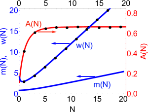
Figure 2: Dependencies of droplet width $w$, the power exponent $m$ (the left axis), and the droplet amplitude $A$ (the right axis) on $N$ for $\gamma=-1$ and $\delta=1$. Lines correspond to the VA, while points are from numerical simulations of Eq. (2).

By eliminating $b$ from Eqs. (10), equation for $w(t)$ is represented as an equation of motion of an effective particle in a potential:

$$w_{tt}=-{\partial U(w)\over\partial w},$$ (13)

where

$$U(w)={1\over\Gamma(3s)}\left[{\Gamma(2-s)\over 8s^{2}w^{2}}-{\gamma N\over 2^{s+2}sw}\right.$$

$$\left.-{2^{s+1}\delta\over 3^{s+1}}\left({N\,\Gamma(s)\over 2sw}\right)^{1/2}\right].$$ (14)

The potential $U(w)$ for $N=1$ and $m=0.971$ is shown in the inset of Fig. (1). For given $N$ and $m$, potential $U(w)$ has a single minimum at $w=w_{s}$ that corresponds to the stationary QD. Potential $U(w)$ tends to zero at large $w$. The VA also describes the dynamics of the QD parameters, when the initial profile is different from the stationary one.

When the initial energy $\mathcal{E}_{0}=w_{t}^{2}(0)/2+U(w_{0})$ of the effective particle is negative, the VA predicts a periodic variation of the QD width (and other parameters), see Eq. (13). However, this picture is true only for small deviations from the stationary QD shape. For moderate deviations ($>$ 20%-30%), numerical simulations of Eq. (2) show a generation of linear waves and a splitting of the initial distribution. This means that a moderately deformed QD breaks into several droplets. Some of these droplets move in opposite directions with the same velocities, such that the total momentum is conserved.

Figure 3: The period of small oscillations $T$ of the QD width, found from Eq. (15) (the line) and from numerical simulations (points) of Eq. (2), as a function of $N$ for $\gamma=-1$ and $\delta=1$. The inset shows a map plot of $|\Psi(x,t)|^{2}$ for $N=5$ , $m_{s}=1.66$ ($A_{s}=0.653$ and $w_{s}=6.54$).

A variation of the QD shape, found from numerical simulations of Eq. (2), is presented in the inset of Fig. 3. Similar to Fig. 2, we change the parameters of the stationary profile by 10 %, and use this profile as an initial condition. We monitor the QD dynamics over $t\sim 800$ and find the period as an average on the last 2-4 oscillations.

We should emphasize that oscillations of the QD shape near the stationary shape are almost undamped. We perform numerical simulations of Eq. (2) up to $t\sim 10000$ ($\sim$ 200 periods), and we do not observe substantial decrease of the oscillation amplitude, after some initial shape adjustment. A sustainability of oscillations is a peculiar property of QDs, and it can be used to distinguish them from the NLS solitons.

By using the potential, we can find the frequency $\Omega_{0}$ of small oscillations of droplet parameters near the stationary state as

$$\Omega_{0}^{2}=\left.{\partial^{2}U(w)\over\partial w^{2}}\right|_{w=w_{s}}.$$ (15)

Figure 3 shows the dependence of the period of oscillations $T=2\pi/\Omega_{0}$ found from Eq. (15) and from numerical simulations.

The dynamics of the QD width, found from numerical simulations of Eq. (2), is compared with predictions of the VA, Eq. (13), in Fig. 4. One can see that for small $N$ ($N=0.2$ in the figure) there is a noticeable difference between the results, see also Fig. 3. For such $N$, the actual profile is different from distribution (7). Therefore, an initial adjustment of the QD shape shifts the phase of oscillations. Nevertheless, there is a reasonable qualitative agreement of results for the amplitude and the period of oscillations. For $N>1$, an agreement between numerical simulations and the VA is good, as seen from Figs. 3 and 4. Results, summarized in Figs. 1-4, shows that the VA correctly predicts not only stationary parameters, but also the dynamics of QDs.

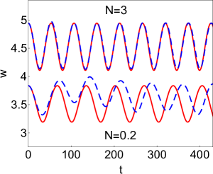
Figure 4: Oscillations of the QD width found from numerical simulations (solid lines) of Eq. (2) and from Eqs. (13) of the VA (dashed lines).

When $\mathcal{E}_{0}>0$, according to Eq. (13), a pulse is broadened infinitely, and disappears. This prediction is valid only qualitatively. Numerical simulations of Eq. (2) indicate that the regime of splitting is replaced by the dispersive broadening for much larger deformations, than the VA predicts. For deformations that preserve $N$, a large deformation corresponds to small values of the distribution area $S=\int_{-\infty}^{\infty}|\psi|dx$. This indicates that there is a threshold value $S_{th}$ such that when $S_{0}<S_{th}$, an initial distribution is broadened. This property is similar to the property of pulses in the NLS model, $\gamma=1$ and $\delta=0$ in Eq. (2), where threshold value is given by $S_{th,NLS}=\pi/2$.

Let us estimate parameters for realistic experiments in a binary BEC of Rb atoms ($m=1.42\cdot 10^{-25}\ \mathrm{kg}$) in spin up and spin down states. For the intra-species scattering length, we take $a_{\uparrow\uparrow}=a_{\downarrow\downarrow}=2000a_{0}$, and assume that the inter-species scattering length $a_{\uparrow\downarrow}\sim-(0.95\mathrm{-}0.99)a_{\uparrow\uparrow}$, where $a_{0}$ is the Bohr radius, so that the residual scattering length satisfies $0<a_{\uparrow\downarrow}+\sqrt{a_{\uparrow\uparrow}a_{\downarrow\downarrow}}\ll\sqrt{a_{\uparrow\uparrow}a_{\downarrow\downarrow}}$ [2]. The transverse radius of a trap is taken as $a_{\bot}=0.6\ \mu\mathrm{m}$. Then, the critical temperature of the Bose condensation for a gas with density $\sim 10^{14}\ \mathrm{cm}^{-3}$ is $T_{cr}=0.7\ \mu\mathrm{K}$. The characteristic scales for a system with $|\gamma|=1$ and $|\delta|=1$ are $x_{s}\sim(1\mathrm{-}0.4)\ \mu\mathrm{m}$, $t_{s}\sim(0.8\mathrm{-}0.2)\ \mathrm{ms}$, and $N_{s}\sim 40\mathrm{-}450$. These parameters are compatible with typical experiments on BECs [11].

As far as we know, there are no experiments on 1D QDs. In experiments on 3D QDs in potassium mixtures [5, 7], a size of QDs is $0.5\mathrm{-}6\ \mu\mathrm{m}$, and the total number of particles $N\sim(2\mathrm{-}25)\!\cdot\!10^{3}$. Our estimation shows that it is more easy to create 1D QDs in BECs with heavier atoms and larger scattering lengths. This motivates our choice of Rb in calculation of characteristic scales.

3 Dynamics of solitons for different values of $\gamma$ and $\delta$

Equation (13) for $w$ with potential (14) allows us to study the dynamics of localized waves for different values of $\gamma$ and $\delta$. In BECs, the sign of $\gamma$ can be changed via the Feshbach resonance, see e.g. [11]. Though only a positive sign of $\delta$ was considered in Ref. [2], here we assume that $\delta$ can have any sign. By normalization of Eq. (2), one can eliminate the dependence on absolute values of the parameters. Therefore, we consider cases, when $\gamma$ and $\delta$ each take one of the three values -1, 0, and 1. When $\delta=0$, we either have a free linear condensate ($\gamma=0$), or a well-studied system of a BEC with the two-body interaction [11]. Since a system with $\gamma<0$ and $\delta>0$ is considered in the previous section, we only need to study five cases. In BEC literature, QDs, localized states in a presence of quantum fluctuations, are distinguished from solitons that exist without fluctuations. However, in this Section, we call all localized states as solitons.

Figure 5: Shapes of potentials for different $\gamma$ and $\delta$. Parameters ($\gamma$, $\delta$, $N$, $m$) for the solid, dashed and dotted lines are (1, 1, 1, 0.842), (-1, -1, 1, 0.971), and (1, -1, 7, 0.782), respectively. The inset shows a scaled-up region (a grey rectangle) around the maximum of the dotted curve.

Typical shapes of the potentials are presented in Fig. 5. All potentials in Fig. 5 tend to zero at $w\to\infty$. For $\delta=1$ and $\gamma=0$, or $\gamma=1$ (the solid line in Fig. 5), the shape of $U(w)$ is the same as presented in the inset of Fig. 1. This means that when $\delta>0$, there exists a stable soliton for any values of $\gamma$. However, there are no flat-top solitons when $\gamma\geq 0$, all solitons are bell-shaped with $m\sim 0.8-0.9$. In particular, for $\gamma=0$ and $\delta=1$, the power exponent $m=0.877$ does not depend on $N$, c.f. Eq. (16).

When $\gamma\leq 0$ and $\delta<0$ (the dashed line in Fig. 5), there are no bright solitons, therefore any initial pulse spreads dispersively. This is not surprising, because for these parameters, both nonlinearities correspond to repulsive self-interaction. For monotonically decreasing potential $U(w)$, there is a question what number $m$ should be used in the dynamical equation (10), since there are no stationary solitons, or proper roots for $m$ in the second of Eqs. (11). In this case, in order to model the dynamics, one can use the initial value $m=m_{0}$ in Eq. (13).

For case $\gamma>0$ and $\delta<0$, there are two choices: (i) when $N<N_{\mathrm{th}}$, no solitons exist (with a form of the potential similar to the dashed line in Fig. 5), (ii) when $N\geq N_{\mathrm{th}}$, two stationary solitons exist, because potential $U(w)$ has two extrema (see the dotted line and an inset in Fig. 5). In fact, for these signs of $\gamma$ and $\delta$, and $N>N_{\mathrm{th}}$, the second of Eqs. (11) has two roots for $m$, however one root corresponds to unstable solitons with $\mu>0$. The threshold value of the norm for $\gamma=1$ and $\delta=-1$ is $N_{\mathrm{th}}\approx 4.2$. As follows from Eq. (14), $U(w)$ tends to zero at $w\to\infty$ from positive values. We also mention that the value of the potential at the minimum can be negative or positive, depending on $N$.

Numerical simulations shows that for $\gamma>0$ and $\delta<0$ there is no splitting of initially deformed solitons. A deformed distribution emits linear waves and adjusts its form to the soliton profile. Also, for large deformations, there is a broadening of initial distributions.

We obtain that the exact solution (4), derived in Ref. [2] for $\gamma<0$ and $\delta>0$, can be generalized for any signs of $\gamma$ and $\delta$, provided that the soliton exists. When $\gamma=0$ and $\delta>0$, solution (4) is reduced to [9, 10]

$$\Psi(x,t)=-{3\mu\over 2\delta}\,\mathrm{sech}^{2}(\sqrt{-\mu/2}\,x)e^{-i\mu t}.$$ (16)

It follows from the analysis of the exact solutions (4) and (16), and also from the VA that solitons are stable in the whole region of existence because $d\mu/dN<0$.

The predictions of the VA are supported by numerical simulations of Eq.(2). Therefore, the VA based on the super-Gaussian function describes well the dynamics of localized states for any values of $\gamma$ and $\delta$.

4 Conclusions

The variational approach based on the super-Gaussian function has been developed for a description of the dynamics of quantum droplets. A comparison of VA predictions with results of numerical simulations shows an excellent agreement for stationary parameters of QDs. The period of small oscillations of the soliton shape has been found. The oscillation period of quantum droplets is much larger than the characteristic time scale. The long-lived oscillations of the QD shape indicates an existence of a linear mode localized on the QD.

It has been demonstrated that the VA provides a correct prediction of existence of stable localized states for any values of $\gamma$ and $\delta$. It has been found that for $\gamma>0$ and $\delta<0$, solitons are formed when the norm exceeds the threshold value. Numerical simulations of Eq. (2) shows a splitting of a moderately deformed QD, and dispersive broadening for large deformations.

Good agreement of theoretical results with numerical simulations show that the super-Gaussian function is close to the actual shape of localized waves in the system. Therefore, this trial function can also be used in the analysis of the droplet dynamics under various perturbations.

References

- [1] D. S. Petrov, Quantum mechanical stabilization of a collapsing Bose-Bose mixture, Phys. Rev. Lett. 115 (2015) 155302.
- [2] D. S. Petrov and G. E. Astrakharchik, Ultradilute low-dimensional liquids, Phys. Rev. Lett. 117 (2016) 100401.
- [3] I. Ferrier-Barbut, H. Kadau, M. Schmitt, M. Wenzel, and T. Pfau, Observation of quantum droplets in a strongly dipolar Bose Gas, Phys. Rev. Lett. 116 (2016) 215301.
- [4] D. Edler, C. Mishra, F. Wachtler, R. Nath, S. Sinha, and L. Santos, Quantum fluctuations in quasi-one-dimensional dipolar Bose-Einstein condensates, Phys. Rev. Lett. 119 (2017) 050403.
- [5] C. R. Cabrera, L. Tanzi, J. Sanz, B. Naylor, P. Thomas, P. Cheiney, L. Tarruell, Quantum liquid droplets in a mixture of Bose-Einstein condensates, Science 359 (2018) 301.
- [6] P. Zin, M. Pylak, T. Wasak, M. Gajda, and Z. Idziaszek, Quantum Bose-Bose droplets at a dimensional crossover, Phys. Rev. A 98 (2018) 051603.
- [7] P. Cheiney, C. R. Cabrera, J. Sanz, B. Naylor, L. Tanzi, and L. Tarruell, Bright soliton to quantum droplet transition in a mixture of Bose-Einstein condensates, Phys. Rev. Lett. 120 (2018) 135301.
- [8] G. E. Astrakharchik and B. A. Malomed, Dynamics of one-dimensional quantum droplets, Phys. Rev. A 98 (2018) 013631.
- [9] B. Liu, H.-F. Zhang, R.-X. Zhong, X.-L. Zhang, X.-Z. Qin, C. Huang, Y.-Y. Li, and B. A. Malomed, Symmetry breaking of quantum droplets in a dual-core trap, Phys. Rev. A 99 (2019) 053602.
- [10] A. Tononi, Y. Wang, and L. Salasnich, Quantum solitons in spin-orbit-coupled Bose-Bose mixtures, Phys. Rev. A 99 (2019) 063618.
- [11] C. J. Pethick and H. Smith, Bose-Einstein Condensation in Dilute Gases (Cambridge Univ. Press, 2011).
- [12] T. D. Lee, K. Huang, and C. N. Yang, Eigenvalues and eigenfunctions of a Bose system of hard spheres and its low-temperature properties, Phys. Rev. 106 (1957) 1135.
- [13] D. Anderson, Variational approach to nonlinear pulse propagation in optical fibers, Phys. Rev. A 27 (1983) 3135.
- [14] M. Karlsson, Optical beams in saturable self-focusing media, Phys. Rev. A 46 (1992) 2726.
- [15] E. N. Tsoy, A. Ankiewicz, and N. Akhmediev, Dynamical models for dissipative localized waves of the complex Ginzburg-Landau equation, Phys. Rev. E 73 (2006) 036621.
- [16] B. B. Baizakov, A. Bouketir, A. Messikh, A. Benseghir, and B. A. Umarov, Variational analysis of flat-top solitons in Bose-Einstein condensates, Int. J. of Mod. Phys. B 25 (2011) 2427.
- [17] N. G. Vakhitov and A. A. Kolokolov, Stationary solutions of the wave equation in a medium with nonlinearity saturation, Radiophys. Quantum Electron. 16 (1973) 783.