Torus Constraints in ANEPD-CXO245: A Compton-thick AGN with Double-Peaked Narrow Lines

Abstract

We report on the torus constraints of the Compton-thick AGN with double-peaked optical narrow line region (NLR) emission lines, ANEPD-CXO245, at $z=0.449$ in the AKARI NEP Deep Field. The unique infrared data on this field, including those from the nine-band photometry over 2-24 $\mu$m with the AKARI Infrared Camera (IRC), and the X-ray spectrum from Chandra allow us to constrain torus parameters such as the torus optical depth, X-ray absorbing column, torus angular width ($\sigma$) and viewing angle ($i$). We analyze the X-ray spectrum as well as the UV-optical-infrared spectral energy distribution (UOI-SED) with clumpy torus models in X-ray (XCLUMPY; Tanimoto et al., 2019) and infrared (CLUMPY; Nenkova et al., 2008) respectively. From our current data, the constraints on $\sigma$–$i$ from both X-rays and UOI show that the line of sight crosses the torus as expected for a type 2 AGN. We obtain a small X-ray scattering fraction ($<0.1$%), which suggests narrow torus openings, giving preference to the bi-polar outflow picture of the double-peaked profile. Comparing the optical depth of the torus from the UOI-SED and the absorbing column density $N_{\rm H}$ from the X-ray spectrum, we find that the gas-to-dust ratio is $\gtrsim 4$ times larger than the Galactic value.

1 Introduction

In the course of our multi-wavelength survey on the AKARI NEP Deep Field (ANEPD), including Chandra X-ray observations (Krumpe et al., 2015; Miyaji et al., 2017), optical spectroscopy (Shogaki, 2018), and early UV-optical-infrared (UOI) spectral energy distribution (SED) analysis (Hanami et al., 2012), we have found an optically type 2 Compton-thick (CT) AGN, ANEPD-CXO245 (hereafter CXO245; $z=0.449$, $[\alpha,\delta]_{\rm J2000}=[17^{\rm h}56^{\rm m}01\fs 69,\,66\arcdeg 35\arcmin 00\farcs 6]$ ), which exhibits double-peak optical emission lines from the AGN Narrow-Line Region (NLR).

About $\sim 1$% of present-day type 2 AGNs show double-peaked narrow line region (NLR) features (Liu et al., 2010). The origin of the double peaked narrow lines can be heterogeneous and may be caused by dual AGNs, wind-driven outflows, radio-jet driven outflows and rotating ring-like NLRs (Müller-Sánchez et al., 2015). To discriminate among these scenarios, AGN torus parameters that can be obtained by the analysis of the X-ray spectrum and/or UOI-SED can give a clue, in particular, to distinguish between the outflow and rotating NLR pictures. In the case of a narrow torus opening, it is more difficult for a rotating ring to cross the ionization cone and the bi-polar picture would be favorable. If the line of sight is almost perpendicular to the polar axis, the two sides of a bi-polar outflow would show similar line-of-sight velocities and in this case, the outflow picture would not be favored. In any case, whether the bi-polar outflows and/or rotating rings are generally associated with highly absorbed CT-AGNs can have implications in their evolution stage. The CT AGNs may be at the stage of starting feedback through outflows or tidally-disrupted in-falling clouds generating a ring-like structure.

Another interesting implication of X-ray spectral and UOI-SED analysis is the gas-to-dust ratio of the AGN torus, since the torus IR emission is from dust whereas the X-ray absorption and reflection are produced by gas (Ogawa et al., 2019; Tanimoto et al., 2019).

In view of these, we conduct an AGN torus analysis of CXO245 both from our Chandra X-ray spectrum as well as the UOI SED taking advantage of the unique mid-IR photometric bands available in ANEPD. In Sect. 2, we summarize the dataset used. In Sect. 3, we summarize the key results from the optical emission lines and explain our methods and results of individual and joint X-ray spectral and UOI SED analyses. Discussions and concluding remarks are made in Sect. 4.

We use $H_{0}=70\,{\rm km\,s^{-1}\,Mpc^{-1}}$, $\Omega_{\rm m}=0.3$, and $\Omega_{\Lambda}=0.7$ throughout this paper.

2 Data

2.1 UV, Optical and Infrared (UOI) Data

This object was found as a result of our AKARI survey on the North Ecliptic Pole (NEP) region (AKARI NEP Deep Field; e.g. Matsuhara et al., 2006), where deep observations with all the nine bands of the InfraRed Camera (IRC; $\lambda_{\rm eff}=$ 2,3,4,7,9,11,15,18 & 24 $\mu$m) were made. Extensive multi-wavelength images have been obtained on this field by ground-based and space-bourne observatories. We use UOI photometric measurements from GALEX (Burgarella et al., 2019), Subaru Telescope Suprime Cam (SCAM) (Murata et al., 2013), Canda-Fracnce-Hawaii Telescope (CFHT) MegaCam and WIRCAM (Oi et al., 2014), and Herschel PACS (Pearson et al., 2019)/SPIRE. The SPIRE data, originally published by Burgarella et al. (2019) has been re-analyzed by Pearson et al. (in prep) and we use the revised photometry. Table 1 shows a summary of the UOI photometry. The optical spectra of CXO245 have been obtained during our KECK (DEIMOS) runs in 2008 and 2011 and reduced by Shogaki (2018) using the DEIMOS DEEP2 reduction pipeline. The spectrum from the 2011 run is shown in Fig. 1.

Table 1: UV-Opt.-IR Photometry Used

Band	$\lambda_{\rm eff}$	Flux	Err.($1\sigma$)	Telescope/Instrument
	${\rm[\mu\,m]}$	[mJy]	[mJy]
NUV	0.229	4.980e-4	8.0e-5	GALEX
u*	0.381	1.061e-3	1.8e-5	CFHT/MEGACAM
B	0.437	2.584e-3	8.8e-6	SUBARU/SCAM
V	0.545	7.553e-3	1.6e-5	SUBARU/SCAM
r	0.651	1.939e-2	1.9e-5	SUBARU/SCAM
NB711	0.712	2.547e-2	3.1e-5	SUBARU/SCAM
i	0.768	3.273e-2	2.3e-5	SUBARU/SCAM
z	0.919	4.526e-2	4.6e-5	SUBARU/SCAM
Y	1.03	7.973e-2	5.1e-4	CFHT/WIRCAM
J	1.25	1.113e-1	9.2e-4	CFHT/WIRCAM
Ks	2.15	1.886e-1	1.0e-3	CFHT/WIRCAM
N2	2.41	2.198e-1	3.1e-3	AKARI/IRC
N3	3.28	1.881e-1	2.2e-3	AKARI/IRC
N4	4.47	1.706e-1	2.0e-3	AKARI/IRC
S7	7.30	4.521e-1	1.4e-2	AKARI/IRC
S9W	9.22	7.238e-1	1.8e-2	AKARI/IRC
S11	10.9	1.036e+0	2.3e-2	AKARI/IRC
L15	16.2	1.562e+0	3.7e-2	AKARI/IRC
L18W	19.8	2.297e+0	4.0e-2	AKARI/IRC
L24	23.4	3.342e+0	8.6e-2	AKARI/IRC
PACS100	100	4.760e+0	1.5e+0	HERSCHEL/PACS
PACS160	160	1.768e+1	4.5e+0	HERSCHEL/PACS
PSW	250	2.974e+1	3.8e+0	HERSCHEL/SPIRE
PMW	350	2.353e+1	2.9e+0	HERSCHEL/SPIRE
PLW	500	1.320e+1	3.7e+0	HERSCHEL/SPIRE

2.2 X-ray Data and Reduction

A major fraction ($\sim 0.25\,{\rm\deg}^{2}$) of ANEPD has been observed with Chandra with a total exposure of $\sim 300{\rm ks}$ (Krumpe et al., 2015). CXO245 is covered by the Chandra ACIS-I FOVs of seven OBSIDs (see Facilities; total exposure $\sim 120$ ks with off-axis angles from 3.3^′ to 9.6^′). The X-ray spectrum of each OBSID has been extracted from a circular region with a radius corresponding to the larger of 50% ECF at 3.5 keV (from the Ciao tool psfsize_srcs) or 3.5^′′. The background spectrum is extracted from an annulus with inner and outer radii of 10.5^′′ and 55^′′ respectively, excluding a $10^{\prime\prime}$ region around another X-ray source (ANEPD-CXO358). A merged source and a background spectra have been generated using the Ciao tool combine_spectrum with the option bscale_method=time. This option generates both the combined source and background spectra in integer counts per bin accompanied by an appropriately weighted mean response matrix and a background scaling factor. These allow us to fit the background subtracted spectrum with full Poisson statistics (for small counts) with the XSPEC option cstat. In our X-ray spectroscopic analysis, we use the merged source spectrum with the supporting files created in this step. The resulting X-ray spectrum is shown in Fig. 2(a) along with the model described in Sect. 3.2.1.

3 Analysis and Results

3.1 Optical Emission Lines

The fluxes of each emission line have been obtained with Gaussian+linear continuum fits. Multiple Gaussian components are used if needed. The details of the line spectral analysis is beyond the scope of this paper. Here we describe the key results of the analysis.

1. The line ratios of [OIII]$\lambda 5007$/H$\beta\sim 10$ and [NII]$\lambda$ 6583/H$\alpha\sim 1.5$ are well inside the AGN regime in the BPT diagnostic diagram (Baldwin et al., 1981). The spectrum shows [NeV]$\lambda 3425$, which is an an-ambiguous indication of the AGN NLR.

2. The line profiles of the [OIII]$\lambda 5007$, H$\beta$, and H$\alpha$ emission features are all well represented by two narrow (FWHM$\sim$150 ${\rm[km\,s^{-1}}]$ each) and a broader (FWHM$\sim$900 ${\rm[km\,s^{-1}]}$) components. The profiles of noisier [NeIII]$\lambda 3869$ and [NeV]$\lambda 3425$ lines also show similar double peaks. Figure 1 (inset) shows the line profile of [OIII]$\lambda 5007$ with the best-fit three-Gaussian components as the best example.

3. The two narrow components are separated by $\sim 500\,{\rm km\,s^{-1}}$ and have similar fluxes. The peak of the broad component is just halfway between the two narrower peaks.

4. The star-formation dominated line [OII]$\lambda 3727$ is single-peaked. Our nominal redshift ($z=0.499$) is based on this line.

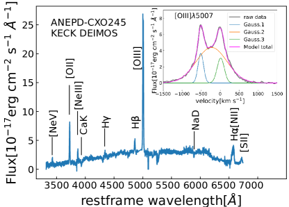
Figure 1: The KECK DEIMOS spectrum of ANEPD-CXO245 from our 2011 in rest frame. The inset shows the profile of the double-peaked [OIII]$\lambda 5007$ emission line from our 2008 spectrum in the radial velocity space with a three-Gaussian decomposition model. The raw data, model total, and each model component are drawn as labeled.

3.2 X-ray Spectrum and IR SED: Torus Analysis

3.2.1 Clumpy Torus: X-ray Spectrum

Current popular models of AGN tori involve dusty-gas media consisting of “clumps” (e.g. Elitzur & Shlosman, 2006; Nenkova et al., 2008).

We first analyze the Chandra spectrum of CXO245 using the new X-ray Clumpy Torus model XCLUMPY (Tanimoto et al., 2019), which has the same geometry and geometrical parameters as the CLUMPY (Nenkova et al., 2008) model. Thus direct comparisons with the results of Sect. 3.2.2 are possible. We use the XSPEC mode of the form:
phabs*(zphabs*cabs*cutoffpl+const*cutoffpl
+atable{xclumpy_R.fits}
+atable{xclumpy_L.fits}).

The first phabs represents the Galactic absorption towards the source direction and its column density is fixed to $N_{\rm H,Gal}=4\times 10^{20}{\rm cm^{-2}}$ (Kalberla et al., 2005). The first and second term in the parenthesis are transmitted and scattered primary continuum respectively. The former is subject to a line-of-sight photoelectric absorption (zphabs) and a Compton scattering (cabs) through the torus. The latter expresses that the fraction $f_{\rm X,sct}$ (represented by a const) is scattered by electrons in thin plasma above and below the polar torus openings. The XSPEC table models xclumpy_R.fits and xclumpy_L.fits provide the continuum and the emission line (including fluorescent emission lines from elements up to $Z=30$, dominated by Fe K$\alpha$) components of the X-ray reflection from the clumpy torus respectively. The normalization and photon index of the primary X-ray continuum are free parameters, where the latter is allowed to vary within $1.5\leq\Gamma\leq 2.5$, while its cutoff energy is fixed to $E_{\rm c}=300\,{\rm keV}$ (Koss et al., 2017; Ricci et al., 2018). These parameters are common to the reprocessed, transmitted, and scattered components. The solar abundance (Anders & Grevesse, 1989) is assumed. The redshift parameter of the model components that require one are fixed to $z=0.449$. Spectral fits are made in channel energies of $0.5-7.0\,{\rm keV}$ using a Markov Chain Monte Carlo (MCMC) chain with the length of 40,000 (using XSPEC’s chain command). In the current version of XCLUMPY, the number of clumps along the equator, the ratio of the outer to inner radii, and the radial clumpy distribution index are fixed to $N_{\rm clump}^{\rm Equ}=10$, $Y=20$, and $q=0.5$ respectively. The parameter ranges covered by the model implementation for the equatorial column density, torus width and viewing angle are $23\leq\log N_{\rm H}^{\rm Equ}\leq 26$, $10\arcdeg\leq\sigma\leq 70\arcdeg$ and $20\arcdeg\leq i\leq 87\arcdeg$ respectively.

Table 2 shows the best-fit parameters and the 90% confidence ranges obtained from the MCMC chain. Figure 2(a) shows the best-fit model and the contribution of various components with the unfolded ACIS spectrum. Figure 2(a) (inset) shows the integrated probability grayscale image and its contours (see caption) in the $\sigma$-$i$ space. Because the available solid angle per viewing angle ($i$) is proportional to $\sin i$, we use $\sin i$ as a prior. Practically, we calculate the 90% ranges from the chain points weighted by the prior. Likewise, the marginal probability in each bin $P_{\rm X}(\sigma_{j},i_{k})$ by accumulating the weighted chain points and normalizing. The integrated probability $I_{\rm X}(\sigma_{j},i_{k})$ is obtained by iterating, in the order of decreasing $P_{\rm X}(\sigma_{j},i_{k})$:

$$I_{\rm X}(\sigma_{j},i_{k})=P_{\rm X}(\sigma_{j},i_{k})+I_{\rm X,prev},$$ (1)

where $I_{\rm X,prev}$ is the integrated probability from the previous step (or 0 in the first step).

The spectrum shows a strong Fe K$\alpha$ line characteristic of a Compton-thick (CT) AGN. The derived column densities (both equatorial and line-of sight) correspond to $N_{\rm H}>10^{24}{\rm cm^{-2}}$ and thus CXO245 can be classified as a CT-AGN. The confidence contours of Fig. 2 and Table 2 show that the line-of-sight viewing angle cannot be too close to the pole ($i>30\arcdeg$; 90% lower limit).

Table 2: Model Parameters

Param.	X-ray Spectrum	UOI SED	Joint
$\log N_{\rm H}^{\rm Equ}$	24.7 (24.5;25.9*)	$\dots$	$\dots$
$\tau_{\rm V}N_{0}$	$\dots$	400(400;400)	$\dots$
$\sigma$	55 (18;69*)	50 (20*;70*)	50 (20*;70*)
$i$	49 (30;85*)	40 (20;90*)	50 (30;80*)
$\Gamma$	2.2 (1.5;2.4)	$\dots$	$\dots$
$\log f_{\rm X,sct}$	-4.0 (-6.0*;-3.0)	$\dots$	$\dots$
$f_{X,15}$	8 (5;9)	$\dots$	$\dots$
$\log L_{\rm X}^{\rm int}$	44.7 (44.4;45.7)	$\dots$	$\dots$
$\log L_{\rm AGN}^{\rm IR}$	$\ldots$	44.6 (44.5;44.8)	$\dots$
$f_{\rm AGN}^{\rm IR}$	$\dots$	0.5 (0.5;0.6)	$\dots$

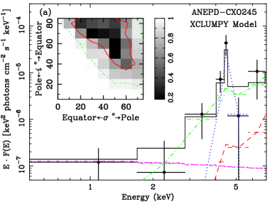
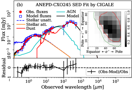
Figure 2: (a) The unfolded $E\cdot F(E)$ representation of our Chandra ACIS-I spectrum of ANEPD-CXO245. The black filled circles with error bars show the observed data binned to at least 2$\sigma$/bin up to 80 ACIS PI channels. The binning is for display only. The solid black histogram shows the best-fit model described in 3.2.1. Also plotted are the reflected continuum (green dot-dashed line), reflected fluorescence line (blue dotted line), transmitted (red dashed line) and scattered (magenta dot-dot-dashed line) components. The inserted box shows the integrated probability image and confidence contours in the $\sigma$ – $i$ space in grids of $10\times 10\,{\rm deg^{2}/pixel}$. The contours correspond to integrated marginal probabilities of 68% (red solid contour) and 95% (green dotted contour). (b) The Optical-IR data fitted with CIGALE with the CLUMPY implementation. The photometry data and best-fit model with the contribution of each component are shown as labeled with residuals. The curve labeled “Dust” refers to the dust emission from star-formation activity, while “AGN” refers to the AGN torus dust emission from CLUMPY. The inset shows the integral probability image and the confidence contours at the same levels as in panel (a).

3.2.2 Clumpy Torus: UV-Optical-Infrared (UOI) SED

We also investigate the AGN torus constraints from the UOI-SED ($\approx 0.2-1000\,{\rm\mu m}$) of CXO245 in the framework of the clumpy torus model CLUMPY (Nenkova et al., 2008). For this purpose, we have made a modification to the CIGALE package (Noll et al., 2009; Boquien et al., 2019) to include an implementation of CLUMPY. To make the consistent analysis with the XCLUMPY X-ray spectrum, we search for best fit parameters assuming $N_{0}=10$, $Y=20$, and $q=0.5$. In the SED fit, we use the galaxy stellar component (Bruzual & Charlot, 2003) with a Salpeter (1955) IMF, double exponentially-decaying star-formation history and an attenuation by (Charlot & Fall, 2000). For the dust emission models, we use the Dale et al. (2014) model for the star-formation and CLUMPY for the AGN torus. The optical part is included in the fits, because the star-formation dust component in the IR and the dust attenuation of the star light are energetically connected. This helps make a better separation of the AGN and star formation IR components.

There are certain limitations in the best-fit and parameter error search in CIGALE. For table models, CIGALE only allows us to evaluate $\chi^{2}$ at the grid points in the table and no interpolations are made, unlike the X-ray spectral analysis using XSPEC. The MCMC is not implemented either. Thus the best fit values and bounds are among these grid points. In our implementation, the grids of the free geometrical parameters are $\sigma=20\arcdeg$–$70\arcdeg$ and $i=0\arcdeg$–$90\arcdeg$ in every 10$\arcdeg$ respectively. A common approach in determining a 90% confidence error range is to use the $\Delta\chi^{2}<2.7$ criterion. However, especially for $\sigma$ and $i$, parameters are often pegged at the model limits and therefore this criterion does not properly indicate the true 90% probability range. Thus, we determine the 90% confidence range $(p-;p+)$ of the parameter $p$ by $C(<p-)\sim 0.05$ and $C(<p+)\sim 0.95$ respectively, where $C$ is the cumulative probability:

$$C(<p)=\frac{\sum_{p_{k}\leq p}\sin i_{k}\exp\left[-\chi^{2}(p_{k})/2\right]}{\sum_{{\rm all\,}k}\sin i_{k}\exp\left[-\chi^{2}(p_{k})/2\right]}.$$ (2)

Due to computational limitations, we take $\chi^{2}(p_{i})$ as the minimum value at $p=p_{i}$ where all other parameters are allowed to vary, rather than the marginal probability, and $i_{k}$ is the best-fit viewing angle when $p$ is fixed to $p_{k}$. The 90% confidence ranges are approximate because of the discreteness of the parameter grid.

Likewise, the probability at each point of the two-parameter space $(\sigma_{j},i_{k})$ is determined by:

$$P_{\rm UOI}(\sigma_{j},i_{k})=\frac{\sin i_{k}\exp\left[-\chi^{2}(\sigma_{j},i_{k})/2\right]}{\sum_{\rm j^{\prime}k^{\prime}}\sin i_{k^{\prime}}\exp\left[-\chi^{2}(\sigma_{j^{\prime}},i_{k^{\prime}})/2\right]},$$ (3)

where $\chi^{2}(\sigma_{j},i_{k})$ is the minimum $\chi^{2}$ value at $(\sigma,i)=(\sigma_{j},i_{k})$ with respect to all other parameters. The sum in the denominator is for all the grid points in ($\sigma,i$). Then the integrated probability $I_{\rm UOI}(\sigma_{j},i_{k})$ is obtained in the same manner as Eq. 1. The resulting best-fit parameters and the 90% confidence ranges in one parameter for the AGN torus are shown in Table 2. Figure 2(b)(inset) shows the integrated probability grayscale image in the grids mentioned above with contours.

3.2.3 X-ray – UOI Joint Torus Constraints

The X-ray spectrum and UOI SED give independent probes of the torus parameters. The AKARI IRC and Chandra observations were made during 2006 and 2010-2011 respectively and we do not expect significant changes in the torus properties between these observations. Thus we also explore the joint constraints of the torus parameters. In the current implementation, the parameters that are common to both XCLUMPY and CLUMPY are $\sigma$ and $i$. The joint probability map is calculated by

$$P_{\rm Joint}(\sigma_{j},i_{k})=\frac{P_{\rm X}(\sigma_{j},i_{k})P_{\rm UOI}(\sigma_{j},i_{k})}{\sum_{j^{\prime}k^{\prime}}P_{\rm X}(\sigma_{j^{\prime}},i_{k^{\prime}})P_{\rm UOI}(\sigma_{j^{\prime}},i_{k^{\prime}})},$$ (4)

where the sum is over all pixels in the $(\sigma,i)$ space. The integrated joint probability image $I_{\rm Joint}$, calculated from $P_{\rm Joint}$ in the same manner as Eq. 1, and is shown in Fig. 3.

We note that the new results by Tanimoto et al. (in prep) on the X-ray and IR clumpy torus analyses of a sample of 10 nearby type 2 AGNs show inconsistencies of $\sigma$ and $i$ values between those obtained by X-ray and IR in some objects. Thus the results of the joint constraints should be used with caution.

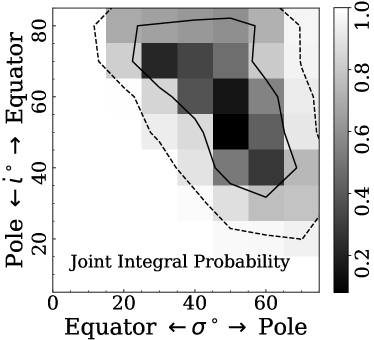
Figure 3: The integrated probability in the $\sigma$–$i$ space from the joint X-ray and UOI analysis. The solid and dashed contours represent 68% and 95% ranges for the two parameters respectively.

4 Discussion and Concluding Remark

The developments of modern AGN torus models, both in the infrared and X-rays, have opened up the possibility of constraining its geometric parameters such as the torus angular width and the viewing angle, in addition to the optical depth (UOI) and the X-ray absorption column density.

In our UOI dataset, $\log L_{\rm AGN}^{\rm IR}$ and $\tau_{\rm V}N_{0}$ are well constrained. We verify that $\log L_{\rm AGN}^{\rm IR}$ changes very little when we use other models of torus and the star formation dust components (Fritz et al., 2006; Schreiber et al., 2016). With CLUMPY, we find $\tau_{\rm V}N_{0}=400$ as the best fit among the model’s grid points and the neighboring grid values of $200$ and $600$ are strongly excluded. In the X-ray analysis, we obtain $N_{\rm H}^{\rm Equ}\gtrsim 4\times 10^{24}{\rm cm^{-2}}$, where the upper bound is unconstrained. Thus we obtain $N_{\rm H}^{\rm Equ}/A_{\rm V}^{Eq}\gtrsim 3\times 10^{21}{\rm cm^{-2}\,mag^{-1}}$ ($A_{\rm V}=2.5\tau_{\rm V}N_{\rm 0}/\ln(10)$). The comparison of this ratio with the Galactic value ($N_{\rm H}/A_{\rm V}=1.87\times 10^{21}{\rm cm^{-2}\,mag^{-1}}$; Draine, 2003), implies that the gas-to-dust ratio of the CXO245 torus is at least 4 times larger than that of the Galaxy. This is consistent with the results from some other works. Tanimoto et al. (2019) has found a gas-to-dust ratio of $\sim 26$ times the Galactic value for the nearby CT-AGN the Circinus galaxy. New results from a systematic study of 10 additional nearby Seyfert 2 galaxies with XCLUMPY and CLUMPY (Tanimoto et al. in prep) include measurements of two other CT-AGNs, one of which shows a larger $N_{\rm H}/A_{\rm V}$ value than the Galactic one. The comparison of the silicate absorption depth $\tau_{9.7}$ at $9.7\,\mu{\rm m}$ and $N_{\rm H}$ by González-Martín et al. (2013) shows systematically higher $N_{\rm H}$ than expected from $\tau_{9.7}$ expected from the Galatctic gas-to-dust ratio for obscured AGNs.

The constraints on $\sigma$ and $i$ are much looser. There are, however, some meaningful constraints. The X-ray analysis strongly excludes $90\arcdeg-i\gtrsim\sigma$, meaning that the line of sight crosses the torus material, as expected for type 2 AGNs. We also obtain a lower limit to the viewing angle ($i>30\arcdeg$), excluding a line of sight that is close to the polar axis. The UOI-SED analysis shows a similar trend.

One of our original motivations of this work was to obtain constraints of these angles to give clues to discriminate between the bi-polar outflow and a rotating ring origins of the double-peaked NLR lines (Sect. 1). The constraints of $i$, and $\sigma$ themselves, neither X-ray spectrum nor UOI-SED can suggest which picture is preferred. On the other hand, the very small scattering fraction ($f_{\rm X}\lesssim 0.1\%$) from our X-ray spectral analysis, suggests a small opening angle (large $\sigma$). While $f_{\rm X}$–$\sigma$ relation has not yet been calibratedUeda et al. (2007); Yamada et al. (2019), the rather small scattering fraction suggests some preference to the bi-polar outflow picture.

The 9-band photometric data with AKARI IRC available in the AKARI NEP Deep and Wide fields have made torus analyses with the UOI SED fit possible for CT AGNs across a wide redshift range. These can then be compared and/or combined with the X-ray torus analysis, as demonstrated in this paper. By the analyses on both sides, we obtain a constraint on the gas-to-dust ratio of the AGN torus and loose constraints on the torus width and viewing angles. We are planning to extend this work to the $\sim 5.4\,{\rm deg}^{2}$ AKARI NEP Wide Field by combining the AKARI IRC and supporting UOI data and the scheduled deep exposures with the recently launched eROSITA/ART-XC (Merloni et al., 2012; Pavlinsky et al., 2018) in the NEP region. That would provide the candidates for further Chandra, XMM-Newton and JWST, and, on a longer timescale, Athena observations.

References

- Anders & Grevesse (1989) Anders, E., & Grevesse, N. 1989, Geochim. Cosmochim. Acta, 53, 197
- Baldwin et al. (1981) Baldwin, J. A., Phillips, M. M., & Terlevich, R. 1981, PASP, 93, 5
- Baloković et al. (2018) Baloković, M., Brightman, M., Harrison, F. A., et al. 2018, ApJ, 854, 42
- Boquien et al. (2019) Boquien, M., Burgarella, D., Roehlly, Y., et al. 2019, A&A, 622, A103
- Bruzual & Charlot (2003) Bruzual, G., & Charlot, S. 2003, MNRAS, 344, 1000
- Burgarella et al. (2019) Burgarella, D., Mazyed, F., Oi, N., et al. 2019, PASJ, 71, 12
- Charlot & Fall (2000) Charlot, S., & Fall, S. M. 2000, ApJ, 539, 718
- Dale et al. (2014) Dale, D. A., Helou, G., Magdis, G. E., et al. 2014, ApJ, 784, 83
- Draine (2003) Draine, B. T. 2003, ARA&A, 41, 241
- Elitzur & Shlosman (2006) Elitzur, M., & Shlosman, I. 2006, ApJ, 648, L101
- Fritz et al. (2006) Fritz, J., Franceschini, A., & Hatziminaoglou, E. 2006, MNRAS, 366, 767
- Goto et al. (2019) Goto, T., Oi, N., Utsumi, Y., et al. 2019, PASJ, 71, 30
- González-Martín et al. (2013) González-Martín, O., Rodríguez-Espinosa, J. M., Díaz-Santos, T., et al. 2013, A&A, 553, A35
- Kalberla et al. (2005) Kalberla, P. M. W., Burton, W. B., Hartmann, D., et al. 2005, A&A, 440, 775
- Koss et al. (2017) Koss, M., Trakhtenbrot, B., Ricci, C., et al. 2017, ApJ, 850, 74
- Krumpe et al. (2015) Krumpe, M., Miyaji, T., Brunner, H., et al. 2015, MNRAS, 446, 911 (K15)
- Hanami et al. (2012) Hanami, H., Ishigaki, T., Fujishiro, N., et al. 2012, PASJ, 64, 70
- Liu et al. (2010) Liu, X., Shen, Y., Strauss, M. A., & Greene, J. E. 2010, ApJ, 708, 427
- Matsuhara et al. (2006) Matsuhara, H., Wada, T., Matsuura, S., et al. 2006, PASJ, 58, 673
- Merloni et al. (2012) Merloni, A., Predehl, P., Becker, W., et al. 2012, arXiv e-prints, arXiv:1209.3114
- Miyaji et al. (2017) Miyaji, T., Krumpe, M., Brunner, H., et al. 2017, Publication of Korean Astronomical Society, 32, 235
- Müller-Sánchez et al. (2015) Müller-Sánchez, F., Comerford, J. M., Nevin, R., et al. 2015, ApJ, 813, 103
- Murata et al. (2013) Murata, K., Matsuhara, H., Wada, T., et al. 2013, A&A, 559, A132
- Nenkova et al. (2008) Nenkova, M., Sirocky, M. M., Ivezić, Ž., et al. 2008, ApJ, 685, 147
- Noll et al. (2009) Noll, S., Burgarella, D., Giovannoli, E., et al. 2009, A&A, 507, 1793
- Ogawa et al. (2019) Ogawa, S., Ueda, Y., Yamada, S., et al. 2019, ApJ, 875, 115
- Oi et al. (2014) Oi, N., Matsuhara, H., Murata, K., et al. 2014, A&A, 566, A60
- Pavlinsky et al. (2018) Pavlinsky, M., Levin, V., Akimov, V., et al. 2018, Proc. SPIE, 106991Y
- Pearson et al. (2019) Pearson, C., Barrufet, L., Campos Varillas, M. d. C., et al. 2019, PASJ, 71, 13
- Ricci et al. (2018) Ricci, C., Ho, L. C., Fabian, A. C., et al. 2018, MNRAS, 480, 1819
- Salpeter (1955) Salpeter, E. E. 1955, ApJ, 121, 161
- Schreiber et al. (2016) Schreiber, C., Elbaz, D., Pannella, M., et al. 2016, A&A, 589, A35
- Shogaki (2018) Shogaki, A., Master Thesis, Kwansei Gakuin University (in Japanese)
- Tanimoto et al. (2019) Tanimoto, A., Ueda, Y., Odaka, H., et al. 2019, ApJ, 877, 95
- Ueda et al. (2007) Ueda, Y., Eguchi, S., Terashima, Y., et al. 2007, ApJ, 664, L79
- Yamada et al. (2019) Yamada, S., Ueda, Y., Tanimoto, A., et al. 2019, ApJ, 876, 96