Scaling the semidefinite program solver SDPB

Abstract

We present enhancements to SDPB, an open source, parallelized, arbitrary precision semidefinite program solver designed for the conformal bootstrap. The main enhancement is significantly improved performance and scalability using the Elemental library and MPI. The result is a new version of SDPB that runs on multiple nodes with hundreds of cores with excellent scaling, making it practical to solve larger problems. We demonstrate performance on a moderate-size problem in the 3d Ising CFT and a much larger problem in the $O(2)$ Model.

1 Introduction

The conformal bootstrap program Ferrara:1973yt ; Polyakov:1974gs for constraining and solving conformal field theories (CFTs) experienced a renaissance a decade ago with the introduction of numerical bootstrap methods Rattazzi:2008pe . Over the past several years, these methods have been further developed, generalized, and improved, leading to many advances in our understanding of CFTs. An example application of numerical bootstrap methods is a high-precision determination of scaling dimensions and OPE coefficients in the 3d Ising CFT ElShowk:2012ht ; El-Showk:2014dwa ; Kos:2014bka ; Simmons-Duffin:2015qma ; Kos:2016ysd ; Komargodski:2016auf ; Simmons-Duffin:2016wlq . See Poland:2018epd ; Chester:2019wfx for recent reviews of numerical bootstrap methods.

The key ingredients in the numerical bootstrap are crossing symmetry of four-point correlation functions and unitarity. The space of solutions to these constraints can be explored numerically using semidefinite programming Poland:2011ey ; Kos:2013tga ; Kos:2014bka ; Simmons-Duffin:2015qma . In Simmons-Duffin:2015qma , one of us (DSD) introduced the semidefinite program solver SDPB, designed for bootstrap applications. SDPB implements a well-known primal-dual interior-point method for solving semidefinite programs doi:10.1137/1.9781611970791 ; alizadeh ; citeulike:3473686 ; Vandenberghe:1995:PPR:213565.213573 ; SDPA ; SDPA2 ; SDPAGMP . Its distinguishing features are:

1. It takes advantage of sparsity patterns in matrices that arise in bootstrap problems;

2. It uses arbitrary-precision arithmetic, making it much more robust (though slower) than machine-precision solvers.

Since its introduction, SDPB 1.0 has been used in approximately 70 works Kos:2016ysd ; Simmons-Duffin:2016wlq ; Kos:2015mba ; Chester:2015qca ; Beem:2015aoa ; Iliesiu:2015qra ; Shimada:2015gda ; Poland:2015mta ; Lemos:2015awa ; Lin:2015wcg ; Chester:2015lej ; Chester:2016wrc ; Behan:2016dtz ; Nakayama:2016jhq ; Iha:2016ppj ; Komargodski:2016auf ; Nakayama:2016knq ; Echeverri:2016ztu ; Paulos:2016fap ; Paulos:2016but ; Li:2016wdp ; Collier:2016cls ; Pang:2016xno ; Lin:2016gcl ; Bae:2016yna ; Bae:2016jpi ; Lemos:2016xke ; Beem:2016wfs ; Li:2017ddj ; Collier:2017shs ; Cornagliotto:2017dup ; Behan:2017emf ; Nakayama:2017vdd ; Iliesiu:2017nrv ; Dymarsky:2017xzb ; Chang:2017xmr ; Cho:2017fzo ; Dymarsky:2017yzx ; Paulos:2017fhb ; Bae:2017kcl ; Dyer:2017rul ; Chester:2017vdh ; Chang:2017cdx ; Cornagliotto:2017snu ; Agmon:2017xes ; Rong:2017cow ; Baggio:2017mas ; Stergiou:2018gjj ; Poland:2018epd ; Liendo:2018ukf ; Rong:2018okz ; Atanasov:2018kqw ; Behan:2018hfx ; Kousvos:2018rhl ; Bae:2018qym ; Bao:2018dzk ; Cappelli:2018vir ; Gowdigere:2018lxz ; Li:2018lyb ; Karateev:2019pvw ; Afkhami-Jeddi:2019zci ; Go:2019lke ; Stergiou:2019dcv ; Lin:2019kpn ; delaFuente:2019hbl ; Homrich:2019cbt ; Manenti:2019kbl ; Gimenez-Grau:2019hez ; Chester:2019wfx ; Agmon:2019imm ; Bercini:2019vme . For example, it played an essential role in the recent high-precision determination of CFT data in the 3d Ising model Kos:2016ysd ; Simmons-Duffin:2016wlq . It has also been used for exploring theories in 2 dimensions delaFuente:2019hbl ; Lin:2015wcg ; Cornagliotto:2017dup ; Collier:2017shs ; Lin:2016gcl , 3 dimensions Iliesiu:2017nrv ; Dymarsky:2017xzb ; Dymarsky:2017yzx ; Atanasov:2018kqw ; Agmon:2019imm ; Kousvos:2018rhl ; Li:2018lyb ; Stergiou:2019dcv ; Agmon:2017xes ; Rong:2017cow ; Baggio:2017mas ; Stergiou:2018gjj ; Chester:2017vdh ; Bae:2016jpi ; Echeverri:2016ztu ; Komargodski:2016auf ; Nakayama:2016jhq ; Chester:2016wrc ; Chester:2015qca ; Iliesiu:2015qra ; Shimada:2015gda ; Kos:2016ysd ; Simmons-Duffin:2016wlq ; Kos:2015mba , 4 dimensions Karateev:2019pvw ; Rong:2018okz ; Poland:2015mta ; Lemos:2015awa ; Manenti:2019kbl ; Cornagliotto:2017snu ; Lemos:2016xke ; Beem:2016wfs ; Li:2017ddj ; Nakayama:2016knq ; Iha:2016ppj , 5 dimensions Chang:2017cdx ; Li:2016wdp , and 6 dimensions Beem:2015aoa ; Chang:2017xmr , as well as theories in fractional dimensions Cappelli:2018vir ; Gowdigere:2018lxz ; Nakayama:2017vdd ; Pang:2016xno ; Chester:2015lej , defect theories Liendo:2018ukf ; Gimenez-Grau:2019hez , and nonlocal theories Behan:2017emf ; Behan:2018hfx , and for studying the modular bootstrap Collier:2016cls ; Bae:2016yna ; Cho:2017fzo ; Bae:2017kcl ; Dyer:2017rul ; Lin:2019kpn ; Afkhami-Jeddi:2019zci ; Bae:2018qym , and the $S$-matrix bootstrap Paulos:2017fhb ; Homrich:2019cbt ; Paulos:2016fap ; Paulos:2016but ; Bercini:2019vme .

Despite the myriad applications of SDPB 1.0, it is easy to find numerical bootstrap problems that are essentially too large for it. A typical crossing symmetry equation can be written in the form

$$\sum_{R,\Delta,\ell}\vec{\lambda}_{R,\Delta,\ell}^{T}V^{I}_{R,\Delta,\ell}(z,\bar{z})\vec{\lambda}_{R,\Delta,\ell} =0,\qquad I=1,\dots,I_{\mathrm{max}}.$$ (1)

Here, $R$ runs over types of operators (e.g., global symmetry representations) appearing in the crossing equation, $\Delta$ runs over scaling dimensions, and $\ell$ runs over spins. The $\vec{\lambda}_{R,\Delta,\ell}$ are vectors of OPE coefficients. $V^{I}_{R,\Delta,\ell}(z,\bar{z})$ are matrices whose entries are functions of the cross-ratios $z,\bar{z}$. The size of a bootstrap computation depends roughly on three quantities:

• The number of crossing equations $I_{\mathrm{max}}$.

• The dimension of the OPE coefficient vectors $\dim(\vec{\lambda}_{R,\Delta,\ell})$ (equivalently, the number of rows or columns in the matrices $V^{I}_{R,\Delta,\ell}$).

• The number of derivatives $\partial_{z}^{m}\partial_{\bar{z}}^{n}$ of the crossing equations used in the semidefinite program. We parameterize the number of derivatives by $\Lambda=\mathrm{max}(m+n)$.

Another measure of complexity is the number of components $N$ of the linear functional applied to the crossing equation (1), which is essentially a function of $I_{\mathrm{max}}$ and $\Lambda$.

As an example, in the computation of the 3d Ising model critical dimensions in Kos:2016ysd , performed using SDPB 1.0, the number of crossing equations used was $I_{\mathrm{max}}=5$, the OPE coefficient vectors were either $1$ or $2$ dimensional, the number of derivatives was $\Lambda=43$, and the resulting linear functional had $N=1265$ components. That computation took approximately 200,000 CPU-hours, spread over 3 weeks. Much larger problems are easy to construct — either by considering larger systems of crossing equations or taking more derivatives. More crossing equations might arise from larger global symmetry groups, from considering four-point functions of operators with spin, from mixing different types of operators, or from a combination of these effects. In addition, more derivatives can lead to higher-precision results, so it is usually desirable to make $\Lambda$ as large as possible.

There are strong hints (from kinks and other features in numerical bootstrap bounds) that a more powerful semidefinite program solver could yield high-precision results for several important theories. With more a powerful solver, new CFTs could potentially become accessible as well. Furthermore, a more powerful solver could yield stronger general constraints on the space of CFTs, for example by improving and combining the bounds of Dymarsky:2017xzb ; Dymarsky:2017yzx on currents and stress tensors in 3d, and enabling generalizations to other spacetime dimensions and symmetry groups.

For these reasons, we have enhanced the semidefinite program solver SDPB to improve performance and scalability. The main changes are the replacement of OpenMP with MPI, which allows computations to scale across hundreds of cores on multiple nodes, and the replacement of MPACK mpack with the Elemental library poulson2013elemental for arbitrary precision distributed linear algebra.

The purpose of this note is to describe some technical details of the changes we have implemented and present performance comparisons between the old version of SDPB (1.0) and the new version (2.0). We do not give a detailed description of the algorithm, since it is the same as in version 1.0 Simmons-Duffin:2015qma . We often refer to Simmons-Duffin:2015qma for notation and definitions.

The structure of this note is as follows. In section 2, we describe our parallelization strategy using MPI and a modified version of the Elemental library. In section 3, we describe changes relative to version 1.0 and verification of correctness. In section 4, we show benchmarks comparing the two versions of SDPB on two different problems. We conclude in section 5 with discussion and future directions.

Code Availability

SDPB is available from the repository at https://github.com/davidsd/sdpb. The figures in this paper were created with version 2.1.3, which has the Git commit hash

• 6b1a5827c7b32481d7ab92fce1935c2f774a4d05

SDPB is written in C++, uses MPI for parallelism, and depends on Boost boost , GMP gmp , MPFR mpfr , and a forked version of Elemental poulson2013elemental . The fork is available at https://gitlab.com/bootstrapcollaboration/elemental. The version associated with this paper has the Git commit hash

• b39d6f5584092c0d56a68d2fc48aa653f0027565

2 Methods

2.1 Elemental and MPI

SDPB solves semidefinite problems using a variety of dense linear algebra operations using arbitrary precision numbers Simmons-Duffin:2015qma . The original implementation relied on the MPACK library mpack for dense linear algebra routines, the GMP library gmp for arbitrary precision numerics, and OpenMP to distribute work to multiple cores. This approach allowed SDPB to scale well up to dozens of cores on a single, shared memory node.

To scale to clusters with hundreds of cores on multiple nodes, we replaced MPACK with the Elemental library poulson2013elemental ; petschow2013high . Elemental implements routines for dense linear algebra on distributed nodes, communicating via MPI. Elemental includes support for arbitrary precision numeric types via the MPFR library mpfr .

MPFR is very careful about correct rounding and exact handling of precision, but, in our tests, ran about half as fast as GMP. SDPB does not require correct rounding or exact handling of precision. For example, it is acceptable for the user to ask for 1000 bits of precision but actually get 1024 bits.

So we forked the Elemental library and replaced the MPFR routines with GMP counterparts. This was not entirely trivial, because GMP does not implement all of the functions that MPFR implements, such as the natural logarithm function log(). For our purposes, where the most complicated linear algebra routines that we use are Cholesky decomposition and eigenvalue computation, the limited special function support in GMP was sufficient.

2.2 Parallelization strategy

To profitably use Elemental and MPI and achieve efficient scaling, we had to partly restructure SDPB so that different cores work independently as much as possible without waiting for each other to finish. For example, we had to be careful when computing global quantities, i.e. quantities that depend simultaneously on information distributed across all cores. An example of a global quantity is the primal error defined below in (3.1), which requires computing a maximum across all blocks of the matrix $P$. If a step of the computation depends on a global quantity, then the remaining steps cannot be started until all cores have finished both computing their contribution to that quantity and communicating that information to each other.

Thus, achieving good performance with MPI required us to be more deliberate when computing anything that requires cores to communicate with one another. Fortunately, most of the operations work on blocks made up of independent groups of matrices. For example, the positive semidefinite matrix $Y$ (one of the internal variables in SDPB) can be written as a block-diagonal matrix

$$Y\equiv\left(\begin{array}[]{cccc}Y_{1}&0&\cdots&0\\ 0&Y_{2}&\cdots&0\\ \vdots&\vdots&\ddots&\vdots\\ 0&0&\cdots&Y_{2J}\end{array}\right),$$ (6)

where each $Y_{i}$ is a submatrix. Each pair of matrices $Y_{2n-1},Y_{2n}$ is associated to a single positivity constraint. Thus, the number of submatrices $2J$ is essentially equal to twice the number of combinations of spins $\ell$ and symmetry representations $R$ appearing in the crossing-symmetry equations (1). For example, for the 3d Ising model computation described in section 4, we have $2J\approx 230$. Each iteration of SDPB involves several basic linear algebra operations involving the matrices $Y_{i}$ and other internal variables. Most of the operations associated with different positivity constraints are independent from each other, and so can be performed on separate cores without synchronization. An exception is the computation of the matrix $Q$, discussed in section 2.2.3.

2.2.1 Block timings

Matrix blocks in SDPB can vary substantially in how much time it takes to operate on them. This can be because the blocks vary dramatically in size, or because large parts of the matrices are identically zero. Working with the number zero in GMP is faster than other numbers. For example, adding zero to a number only requires copying the number, while adding general arbitrary precision numbers takes dramatically longer. The structure of zeros within a block can be quite complicated, making it difficult to create a priori estimates of how expensive each block is.

Because computation times are difficult to predict, we instead directly measure the time for the operations for each block. For each block, it turns out to be sufficient to measure the time to compute its contribution to $Q=B^{T}L^{-T}L^{-1}B$ (see Equation 2.44 in Simmons-Duffin:2015qma ). In detail, this is the sum of the time to perform

• The Cholesky decomposition $S_{pq}=L_{pq}L_{pq}^{T}$, where $S_{pq}={\rm Tr}\left(A_{p}X^{-1}A_{q}Y\right)$,

• The matrix solve $L_{pq}^{-1}B$,

• The matrix multiplication $B^{T}L_{pq}^{-T}L_{pq}^{-1}B$.

During the first iteration of the solver, many numbers are still zero, so the first iteration is usually faster than subsequent iterations. We have observed that timings become stable after the first step, so we collect timings from the second step. For these timing runs, the blocks are distributed in a simple round-robin manner to all of the cores, with a single core usually having many blocks. We write those block timings to a file. Then we restart the calculation and use those timings to allocate blocks to cores.

If there is no block timings file, SDPB will automatically perform a timing run and restart. When starting from a checkpoint, such as when hot-starting Go:2019lke , SDPB will reuse block timings. So a timing run only happens when starting a new calculation from scratch. Block timings can also be manually copied from previous calculations with the same structure.

2.2.2 Load balancing

The problem at this point is then how to distribute blocks among cores and nodes. This turns into a variant of the well-known problem of bin-packing binpacking . We want the most expensive blocks to get more cores allocated to them. However, we still want to keep the work for a single block on a single node, since latency and bandwidth between nodes is much worse than within a node.

The algorithm we use is a variant of Worst-Fit worstfit . We assume that the cluster that SDPB is running on has $N$ identical nodes with $c$ cores each, totaling $C=N\times c$ cores. Starting with all of the individual block timings $t_{{\rm block}}$, we add them up to get a total time

$$t_{{\rm total}}\equiv\sum_{\rm block}t_{{\rm block}}.$$ (7)

Dividing this by $C$ gives us an average time per core

$$t_{{\rm average}}\equiv\frac{t_{{\rm total}}}{C}.$$ (8)

We sort the blocks by their timings $t_{{\rm block}}$ and start with the most expensive blocks. If the timing of a block is greater than the average block time $t_{{\rm block}}>t_{{\rm average}}$, then that block will get $t_{{\rm block}}/t_{{\rm average}}$ cores, rounded down.

A block is assigned to nodes that have the most cores left. If there are no nodes left that have enough spare cores, then the block is squeezed into the node with the most cores left. This is the part that is like Worst-Fit, since we assign blocks to the nodes with the most available cores, rather than nodes with the least available cores that can still fit each block.

This assigns all blocks with $t_{{\rm block}}>t_{{\rm average}}$. Starting with the largest remaining blocks, blocks are collected until the sum of their timings is greater than or equal to the average timing. That collection of blocks is then assigned to a single core. The core will be on the node with the most remaining cores left. This process is continued until all blocks are assigned.

This process necessarily underprovisions blocks, leaving left-over cores on some nodes. These left-over cores are assigned, one-by-one, to the block or collection of blocks with the highest timings per core. For example, consider a setup with a node with 1 large block with $t_{{\rm block}\,1}=5$ that has two cores assigned to it (so $c_{{\rm block\,1}}=2$). In addition, that node has a collection of 2 smaller blocks with

$$\begin{array}[]{ccc}t_{{\rm collection}}&=&t_{{\rm block\,2}}+t_{{\rm block\,3}}\\ t_{{\rm block\,2}}&=&1.2\\ t_{{\rm block\,3}}&=&0.8\end{array}$$ (12)

assigned to a single core. A left over-core would be assigned to the large block, because

$$\frac{t_{{\rm block\,1}}}{c_{{\rm block\,1}}}=\frac{5}{2}>\frac{t_{{\rm collection}}}{c_{{\rm collection}}}=\frac{1.2+0.8}{1}.$$ (13)

For a second left-over core, the respective timings are 5/3 and 2. In that case, the collection is split in two, with each block getting a single core. For a third left-over core, the respective timings are 5/3, 1.2/1, and 0.8/1. So the third core is assigned to the large block.

This is by no means the most optimal solution. For example, when the block collections are split up, they are not rebalanced amongst all the collections on that node. Also, when a large block is squeezed into a node, the existing blocks and block collections do not give up any cores to make the distribution more equitable. In practice, we have observed a maximum imbalance of a factor of 2 between the work assigned to cores. This arises when there are two similar sized blocks, each assigned one core. An extra core is assigned to one of the blocks and not the other. This effect diminishes with larger core counts, as the effect of a single core is less decisive. For the benchmarks in section 4, we observed imbalance factors ranging from 1.02 to 1.2.

2.2.3 Global operations

There are relatively few cases where there is a truly global operation involving all of these different blocks. One significant case is in computing and subsequently inverting the matrix $Q$, implemented as a globally distributed Elemental matrix. When creating $Q$, every block contributes to every every element of $Q$. So we compute the individual contributions of each group of cores to $Q$.

We then perform a global reduce and scatter to sum all of the contributions and distribute the results to the distributed version of $Q$. However, we found that if we used the builtin implementation of the function MPI_Reduce_scatter() message2012mpi , the MPI library would allocate extra copies of $Q$ on each core for sending, receiving, and summing. When running on many cores, these extra copies of $Q$ dominate the use of memory. For large problems, this extra memory usage could make it impossible to run SDPB.

To work around this, we reimplemented MPI_Reduce_scatter(). In particular, we implemented the ring algorithm as found in OpenMPI gabriel04:_open_mpi . This allowed us to tightly control the amount of memory used for temporary objects. This hand-rolled implementation causes some degradation in performance for larger jobs (>50 cores), but it has dramatically reduced the memory usage.

With the global reduce and scatter completed, we use Elemental routines to compute the Cholesky decomposition of $Q$ and distribute the result to all of the different groups of cores.

2.2.4 Memory Optimization

While these changes did improve performance and scalability, they came at the cost of significantly larger memory use. The memory to store individual blocks is well distributed among the cores. So the memory dedicated to blocks is more or less identical between SDPB 2.0 and SDPB 1.0. However, as discussed in Section 2.2.3, there is a global matrix $Q$ that gets contributions from every block. In SDPB 1.0, there is only one copy of this matrix. In SDPB 2.0, there is a copy of the local contribution to $Q$ on every core. These contributions are then added up to make the global $Q$. While $Q$ itself is not the largest internal matrix that the solver uses, all of these copies of $Q$ end up requiring significant amounts of memory.

To mitigate this, we have added an option procGranularity. The main effect of this option is to store fewer copies of $Q$ split up among the cores. Using this option makes the memory usage nearly equivalent to the OpenMP version, but also makes the MPI version (2.0) as slow as or slower than the OpenMP version.

3 Comparisons with version 1.0

3.1 Change to primal error

In the original SDPB paper Simmons-Duffin:2015qma , the primal error is defined as

$${\rm primalError} \equiv\max\left\{\left|p_{i}\right|,\left|P_{ij}\right|\right\},$$

$$P \equiv\sum_{i}A_{i}x_{i}-X,$$

$$p \equiv b-B^{T}x.$$ (14)

It turns out that SDPB 1.0 instead implemented

$${\rm primalError}\equiv\max\left\{\left|P_{ij}\right|\right\},$$ (15)

i.e. leaving out the contribution from the primal error vector $p$. By contrast, in SDPB 2.0 we have implemented (3.1). Fortunately, the impact of this change appears to be minimal. In most cases we have checked, if SDPB 1.0 finds a primal-dual optimal or primal feasible solution, then the missing part of ${\rm primalError}$, $\left|p_{i}\right|$, is extremely small, and consequently doesn’t affect the actual value of ${\rm primalError}$. For cases where $\left|P_{i}\right|$ is not small, then it does not matter if $\left|p_{i}\right|$ is small or not.

For the case where there is only a primal solution, we have found that if $\max\left\{\left|P_{i}\right|\right\}$ has converged, then $\max\left\{\left|p_{i}\right|\right\}$ will eventually converge. Usually it converges earlier, but sometimes, especially if starting from a previous checkpoint Go:2019lke , it can converge later.

As an additional optimization, we removed the “Cholesky stabilization” method described in Simmons-Duffin:2015qma . The purpose of this method was to decrease the condition number of $Q$ before inverting it by adding low-rank contributions (and subtracting off their effects later). This method increases the size of $Q$, slowing down the computation. After experience with SDPB, we recommend that users simply increase precision if they encounter numerical stability issues. This also slows down the computation, but in practice less so than Cholesky stabilization. When initializing the Schur complement solver, removing Cholesky stabilization also allowed us to use a Cholesky decomposition, rather than an LU decomposition, of the $Q$ matrix. This optimization has a small, but noticeable, effect on the total time.

3.2 Correctness check

To ensure that no errors were introduced when upgrading SDPB, we ran a number of problems with both the old and new versions. One example problem is a feasibility search in the 3d Ising model. After two steps, for runs with 200 decimal digits of accuracy; the typical difference was around the 180th digit. Some differences are expected, since the exact nature and order of operations to compute quantities like eigenvalues and Cholesky decompositions will be different between MPACK and Elemental. This comparison gives evidence that the basic linear algebra operations are the same between the two versions. The differences between numbers in the old and new versions increase with more iterations. After 100 iterations, the exact values can be quite different in low decimal places. However, both versions do arrive at the same solution. For optimizations (as opposed to feasibility searches), where the solver is used to minimize or maximize some quantity by finding a primal-dual solution, both versions found the same result to high accuracy (80 digits).

4 Benchmarks

To demonstrate improved performance and scalability, we have benchmarked the new and original versions. All benchmarks were performed on the Grace cluster at Yale. Each node in the Infiniband networked cluster is a Lenovo nx360b, containing 28 cores across two Intel E5-2660 v4 CPU’s and a total of 247 GB of memory. The first benchmark is the semidefinite program described in Kos:2014bka ; Simmons-Duffin:2015qma that arises from studying four-point functions of the $\sigma$ and $\epsilon$ operators in the 3d Ising model. In the notation of the introduction, it involves $I_{\mathrm{max}}=5$ crossing equations, OPE coefficient vectors of size $\dim(\vec{\lambda}_{R,\Delta,\ell})\in\{1,2\}$, maximum derivative order $\Lambda=43$, and a functional with $N=1265$ components. The second, larger, benchmark, described in Go:2019lke ; O2Future , arises from studying four-point functions of the leading-dimension charge-0, 1, and 2 scalar operators in the $O(2)$ model. It involves $I_{\mathrm{max}}=22$ crossing equations, OPE coefficient vectors of size $\dim(\vec{\lambda}_{R,\Delta,\ell})\in\{1,2,3\}$, maximum derivative order $\Lambda=35$, and a functional with $N=3762$ components. Both benchmarks were run with 1216 bits of precision. We measure the time to compute the second iteration, which, as noted in Section 2.2.1, we have found to be a stable and accurate measurement of the overall performance of the solver.

Figure 1 and Table 1 demonstrate that SDPB 2.0 is always faster, with the difference becoming more dramatic at higher core counts. At low core counts, the remaining difference is largely due to using a Cholesky decomposition rather than an LU decomposition (see Section 3.1).

The scaling of SDPB 2.0 is quite good, and gets better for larger problems. The performance does drop off at high core counts, most likely due to our memory-optimized version of MPI_Reduce_scatter() (Section 2.2.3).

Figure 2 and Table 2 show the maximum memory required on a node. SDPB 1.0’s memory use is relatively constant. SDPB 2.0 uses significantly more memory, continually increasing with the number of cores per node. At higher node counts, the memory use per node stabilizes. The computation was able to fit on the available nodes, so we did not use the memory optimization flag detailed in section 2.2.4.

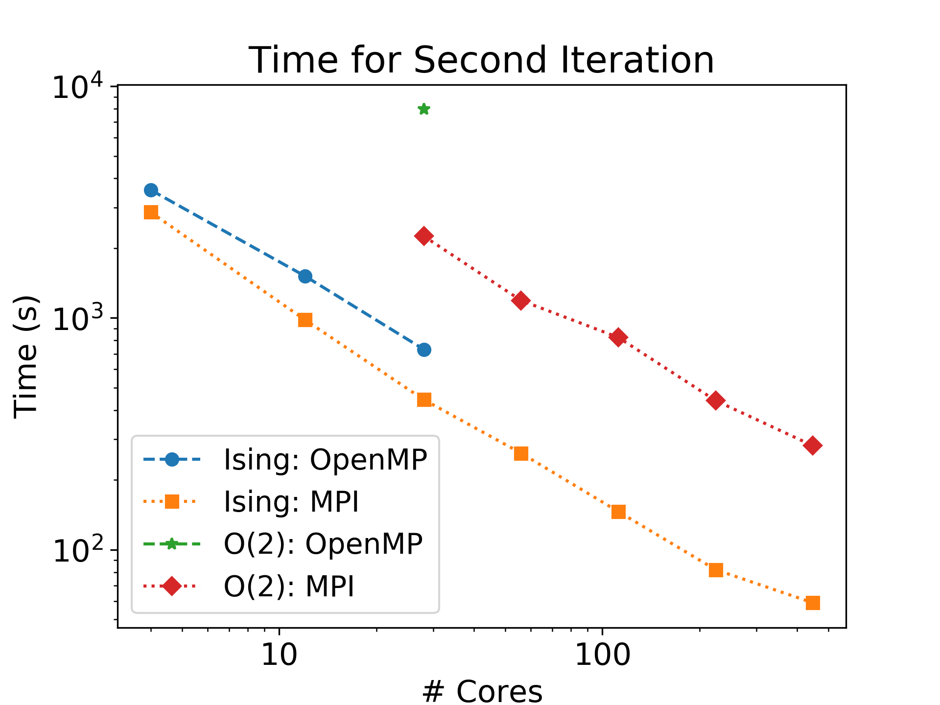
Figure 1: Time to compute the second iteration of an Ising model with 117 blocks (as in Simmons-Duffin:2015qma ) and an O(2) model with 261 blocks on the Yale Grace cluster. SDPB 1.0 is limited to the number of cores on a single node (28), while SDPB 2.0 can scale across multiple nodes.

3d Ising	$O(2)$
#Cores OpenMP MPI 4 3568 2861 12 1517 982 28 732 444 56 261 112 146 224 82 448 59	#Cores OpenMP MPI 28 7950 2254 56 1190 112 824 224 440 448 281

Table 1: Time (s) to compute iterations in Figure 1

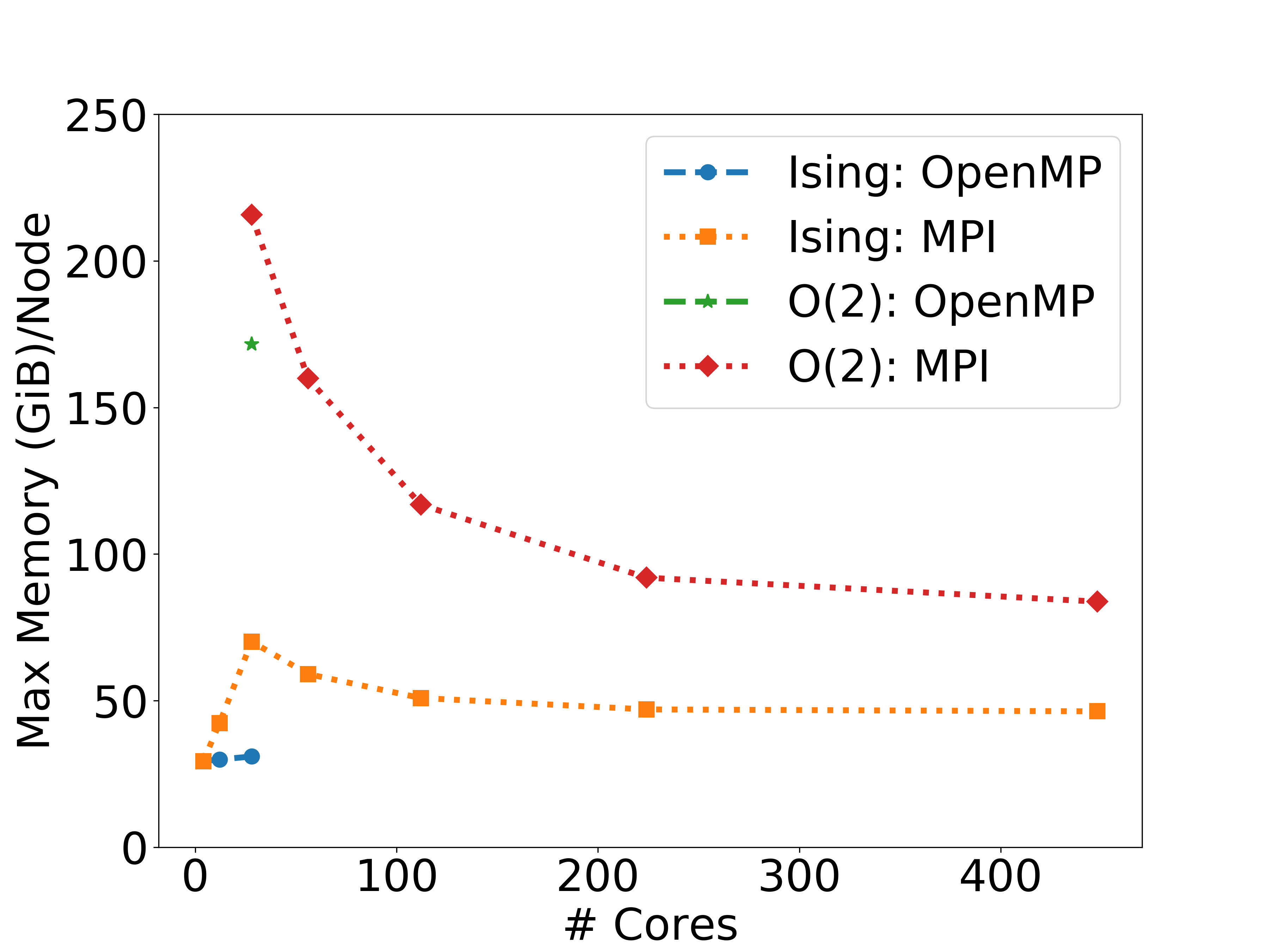
Figure 2: Maximum memory used on a node for the computation in Figure 1.

3d Ising	$O(2)$
#Cores OpenMP MPI 4 29.4 29.3 12 29.9 42.3 28 31.0 70.1 56 59.1 112 50.9 224 47.0 448 46.4	#Cores OpenMP MPI 28 172 216 56 160 112 117 224 92.0 448 83.8

Table 2: Maximum memory (GiB) used on a node for the computation in Figure 1

5 Future directions

We have modified SDPB to use MPI and the Elemental library, and demonstrated that it scales well up to hundreds of cores. There are several interesting directions for future optimizations and improvement. Perhaps the most urgent is to decrease the precision required for numerical bootstrap computations. In practice, large-scale computations require approximately 1000 bits of precision — roughly 20 times what is used in IEEE double precision arithmetic (53 bits for the mantissa). The exact reasons why such precision is necessary are currently unknown, but we do notice that matrices internal to SDPB develop very large condition numbers during computations. Inverting or Cholesky-decomposing these matrices causes instabilities if the precision of the arithmetic is too low. For example, the blocks of the “Schur complement” matrix $S_{pq}$ (see section 2.2.1) can develop condition numbers of size $10^{400}$, while the condition number of $Q$ can reach $10^{100}$. This suggests that a clever change of basis for both the primal and the dual problems might be necessary to mitigate precision issues.

Even with a clever change of basis, we still expect it would be extremely difficult to use machine-precision arithmetic in numerical bootstrap computations. This would require a far more detailed understanding of solutions to crossing symmetry than we currently possess. Historically, high precision has been a powerful tool for circumventing these issues and simply getting things done. One possible future direction is to dynamically change precision based on the size of the problem and the needs of the solver, with less delicate parts of the computation running at lower precision. Precision could be increased slowly over multiple iterations, so that high precision is only used near the end of the computation when condition numbers are largest. (This particular optimization may be less useful in conjunction with hot-starting Go:2019lke ; O2Future .) More optimistically, perhaps high condition numbers and numerical instabilities can be avoided using a different semidefinite programming algorithm, or alternative optimization methods.

Another challenge for SDPB is to scale to even larger machines and larger problems. As one example, our implementation of MPI_Reduce_scatter() could certainly be optimized. Comparing our hand-rolled version with the OpenMPI implementation, there is no obvious reason that our implementation is slower at high core counts. This points to a general need to revisit other communication and synchronization procedures in MPI and optimize them for our use case.

Modern high performance computing clusters often include GPUs, which are in principle well-suited for highly parallel linear algebra operations. We could leverage existing libraries for high-precision linear algebra on GPUs 10.1007/978-3-319-42432-3_29 ; CUMP .

SDPB 1.0 demonstrated the usefulness of a robust optimization tool specialized for numerical bootstrap applications. We hope that SDPB 2.0 will demonstrate the usefulness of scaling such a specialized tool to large problems. In the meantime, it is worthwhile to explore other optimization methods that might prove more efficient in the asymptotic future. The design of SDPB 1.0 was based on the interior point method implemented in SDPA SDPA ; SDPA ; SDPAGMP . Perhaps other SDP algorithms like the multiplicative weight method Arora:2016:CPA:2906142.2837020 suggested in Bao:2018dzk could be more efficient, or circumvent the precision problems of interior point methods. Perhaps the primal-dual simplex method of El-Showk:2014dwa ; Paulos:2014vya can be adapted to work with matrix positivity conditions. The implementation of El-Showk:2014dwa dealt inefficiently with double-roots of extremal functionals. Perhaps it can be modified to allow roots to move continuously, incorporating ideas from El-Showk:2016mxr ; Afkhami-Jeddi:2019zci . While these are superficially engineering problems, their solutions could have deep implications and broad consequences for our understanding of strongly-coupled field theories.

References

- (1) S. Ferrara, A. F. Grillo and R. Gatto, Tensor representations of conformal algebra and conformally covariant operator product expansion, Annals Phys. 76 (1973) 161–188.
- (2) A. M. Polyakov, Nonhamiltonian approach to conformal quantum field theory, Zh. Eksp. Teor. Fiz. 66 (1974) 23–42.
- (3) R. Rattazzi, V. S. Rychkov, E. Tonni and A. Vichi, Bounding scalar operator dimensions in 4D CFT, JHEP 12 (2008) 031, [0807.0004].
- (4) S. El-Showk, M. F. Paulos, D. Poland, S. Rychkov, D. Simmons-Duffin and A. Vichi, Solving the 3D Ising Model with the Conformal Bootstrap, Phys. Rev. D86 (2012) 025022, [1203.6064].
- (5) S. El-Showk, M. F. Paulos, D. Poland, S. Rychkov, D. Simmons-Duffin and A. Vichi, Solving the 3d Ising Model with the Conformal Bootstrap II. c-Minimization and Precise Critical Exponents, J. Stat. Phys. 157 (2014) 869, [1403.4545].
- (6) F. Kos, D. Poland and D. Simmons-Duffin, Bootstrapping Mixed Correlators in the 3D Ising Model, JHEP 11 (2014) 109, [1406.4858].
- (7) D. Simmons-Duffin, A Semidefinite Program Solver for the Conformal Bootstrap, JHEP 06 (2015) 174, [1502.02033].
- (8) F. Kos, D. Poland, D. Simmons-Duffin and A. Vichi, Precision Islands in the Ising and Models, JHEP 08 (2016) 036, [1603.04436].
- (9) Z. Komargodski and D. Simmons-Duffin, The Random-Bond Ising Model in 2.01 and 3 Dimensions, J. Phys. A50 (2017) 154001, [1603.04444].
- (10) D. Simmons-Duffin, The Lightcone Bootstrap and the Spectrum of the 3d Ising CFT, JHEP 03 (2017) 086, [1612.08471].
- (11) D. Poland, S. Rychkov and A. Vichi, The Conformal Bootstrap: Theory, Numerical Techniques, and Applications, Rev. Mod. Phys. 91 (2019) 15002, [1805.04405].
- (12) S. M. Chester, Weizmann Lectures on the Numerical Conformal Bootstrap, 1907.05147.
- (13) D. Poland, D. Simmons-Duffin and A. Vichi, Carving Out the Space of 4D CFTs, JHEP 05 (2012) 110, [1109.5176].
- (14) F. Kos, D. Poland and D. Simmons-Duffin, Bootstrapping the vector models, JHEP 06 (2014) 091, [1307.6856].
- (15) Y. Nesterov and A. Nemirovskii, Interior-Point Polynomial Algorithms in Convex Programming. Society for Industrial and Applied Mathematics, 1994, 10.1137/1.9781611970791.
- (16) F. Alizadeh, Combinatorial Optimization with Interior Point Methods and Semidefinite Matrices, Ph.D. thesis, University of Minnesota, Mineapolis, MN (1991) .
- (17) C. Helmberg, F. Rendl, R. J. Vanderbei and H. Wolkowicz, An interior-point method for semidefinite programming, SIAM Journal on Optimization 6 (1996) 342–361.
- (18) L. Vandenberghe and S. Boyd, A primal-dual potential reduction method for problems involving matrix inequalities, Math. Program. 69 (July, 1995) 205–236.
- (19) M. Yamashita, K. Fujisawa, M. Fukuda, K. Nakata and M. Nakata, A high-performance software package for semidefinite programs: SDPA 7, Research Report B-463, Dept. of Mathematical and Computing Science, Tokyo Institute of Technology, Tokyo, Japan (2010) .
- (20) M. Yamashita, K. Fujisawa and M. Kojima, Implementation and evaluation of SDPA 6.0 (SemiDefinite Programming Algorithm 6.0), Optimization Methods and Software 18 (2003) 491–505.
- (21) M. Nakata, A numerical evaluation of highly accurate multiple-precision arithmetic version of semidefinite programming solver: SDPA-GMP, -QD and -DD., 2010 IEEE International Symposium on Computer-Aided Control System Design (CACSD) (Sept, 2010) 29–34.
- (22) F. Kos, D. Poland, D. Simmons-Duffin and A. Vichi, Bootstrapping the O(N) Archipelago, JHEP 11 (2015) 106, [1504.07997].
- (23) S. M. Chester, S. Giombi, L. V. Iliesiu, I. R. Klebanov, S. S. Pufu and R. Yacoby, Accidental Symmetries and the Conformal Bootstrap, JHEP 01 (2016) 110, [1507.04424].
- (24) C. Beem, M. Lemos, L. Rastelli and B. C. van Rees, The (2, 0) superconformal bootstrap, Phys. Rev. D93 (2016) 025016, [1507.05637].
- (25) L. Iliesiu, F. Kos, D. Poland, S. S. Pufu, D. Simmons-Duffin and R. Yacoby, Bootstrapping 3D Fermions, JHEP 03 (2016) 120, [1508.00012].
- (26) H. Shimada and S. Hikami, Fractal dimensions of self-avoiding walks and Ising high-temperature graphs in 3D conformal bootstrap, J. Statist. Phys. 165 (2016) 1006, [1509.04039].
- (27) D. Poland and A. Stergiou, Exploring the Minimal 4D SCFT, JHEP 12 (2015) 121, [1509.06368].
- (28) M. Lemos and P. Liendo, Bootstrapping chiral correlators, JHEP 01 (2016) 025, [1510.03866].
- (29) Y.-H. Lin, S.-H. Shao, D. Simmons-Duffin, Y. Wang and X. Yin, = 4 superconformal bootstrap of the K3 CFT, JHEP 05 (2017) 126, [1511.04065].
- (30) S. M. Chester, L. V. Iliesiu, S. S. Pufu and R. Yacoby, Bootstrapping Vector Models with Four Supercharges in , JHEP 05 (2016) 103, [1511.07552].
- (31) S. M. Chester and S. S. Pufu, Towards bootstrapping QED3, JHEP 08 (2016) 019, [1601.03476].
- (32) C. Behan, PyCFTBoot: A flexible interface for the conformal bootstrap, Commun. Comput. Phys. 22 (2017) 1–38, [1602.02810].
- (33) Y. Nakayama and T. Ohtsuki, Conformal Bootstrap Dashing Hopes of Emergent Symmetry, Phys. Rev. Lett. 117 (2016) 131601, [1602.07295].
- (34) H. Iha, H. Makino and H. Suzuki, Upper bound on the mass anomalous dimension in many-flavor gauge theories: a conformal bootstrap approach, PTEP 2016 (2016) 053B03, [1603.01995].
- (35) Y. Nakayama, Bootstrap bound for conformal multi-flavor QCD on lattice, JHEP 07 (2016) 038, [1605.04052].
- (36) A. Castedo Echeverri, B. von Harling and M. Serone, The Effective Bootstrap, JHEP 09 (2016) 097, [1606.02771].
- (37) M. F. Paulos, J. Penedones, J. Toledo, B. C. van Rees and P. Vieira, The S-matrix bootstrap. Part I: QFT in AdS, JHEP 11 (2017) 133, [1607.06109].
- (38) M. F. Paulos, J. Penedones, J. Toledo, B. C. van Rees and P. Vieira, The S-matrix bootstrap II: two dimensional amplitudes, JHEP 11 (2017) 143, [1607.06110].
- (39) Z. Li and N. Su, Bootstrapping Mixed Correlators in the Five Dimensional Critical O(N) Models, JHEP 04 (2017) 098, [1607.07077].
- (40) S. Collier, Y.-H. Lin and X. Yin, Modular Bootstrap Revisited, JHEP 09 (2018) 061, [1608.06241].
- (41) Y. Pang, J. Rong and N. Su, theory with F4 flavor symmetry in dimensions: 3-loop renormalization and conformal bootstrap, JHEP 12 (2016) 057, [1609.03007].
- (42) Y.-H. Lin, S.-H. Shao, Y. Wang and X. Yin, (2, 2) superconformal bootstrap in two dimensions, JHEP 05 (2017) 112, [1610.05371].
- (43) J.-B. Bae, K. Lee and S. Lee, Bootstrapping Pure Quantum Gravity in AdS3, 1610.05814.
- (44) J.-B. Bae, D. Gang and J. Lee, 3d minimal SCFTs from Wrapped M5-branes, JHEP 08 (2017) 118, [1610.09259].
- (45) M. Lemos, P. Liendo, C. Meneghelli and V. Mitev, Bootstrapping superconformal theories, JHEP 04 (2017) 032, [1612.01536].
- (46) C. Beem, L. Rastelli and B. C. van Rees, More superconformal bootstrap, Phys. Rev. D96 (2017) 046014, [1612.02363].
- (47) D. Li, D. Meltzer and A. Stergiou, Bootstrapping mixed correlators in 4D = 1 SCFTs, JHEP 07 (2017) 029, [1702.00404].
- (48) S. Collier, P. Kravchuk, Y.-H. Lin and X. Yin, Bootstrapping the Spectral Function: On the Uniqueness of Liouville and the Universality of BTZ, JHEP 09 (2018) 150, [1702.00423].
- (49) M. Cornagliotto, M. Lemos and V. Schomerus, Long Multiplet Bootstrap, JHEP 10 (2017) 119, [1702.05101].
- (50) C. Behan, L. Rastelli, S. Rychkov and B. Zan, A scaling theory for the long-range to short-range crossover and an infrared duality, J. Phys. A50 (2017) 354002, [1703.05325].
- (51) Y. Nakayama, Bootstrap experiments on higher dimensional CFTs, Int. J. Mod. Phys. A33 (2018) 1850036, [1705.02744].
- (52) L. Iliesiu, F. Kos, D. Poland, S. S. Pufu and D. Simmons-Duffin, Bootstrapping 3D Fermions with Global Symmetries, JHEP 01 (2018) 036, [1705.03484].
- (53) A. Dymarsky, J. Penedones, E. Trevisani and A. Vichi, Charting the space of 3D CFTs with a continuous global symmetry, 1705.04278.
- (54) C.-M. Chang and Y.-H. Lin, Carving Out the End of the World or (Superconformal Bootstrap in Six Dimensions), JHEP 08 (2017) 128, [1705.05392].
- (55) M. Cho, S. Collier and X. Yin, Genus Two Modular Bootstrap, JHEP 04 (2019) 022, [1705.05865].
- (56) A. Dymarsky, F. Kos, P. Kravchuk, D. Poland and D. Simmons-Duffin, The 3d Stress-Tensor Bootstrap, JHEP 02 (2018) 164, [1708.05718].
- (57) M. F. Paulos, J. Penedones, J. Toledo, B. C. van Rees and P. Vieira, The S-matrix Bootstrap III: Higher Dimensional Amplitudes, 1708.06765.
- (58) J.-B. Bae, S. Lee and J. Song, Modular Constraints on Conformal Field Theories with Currents, JHEP 12 (2017) 045, [1708.08815].
- (59) E. Dyer, A. L. Fitzpatrick and Y. Xin, Constraints on Flavored 2d CFT Partition Functions, JHEP 02 (2018) 148, [1709.01533].
- (60) S. M. Chester, L. V. Iliesiu, M. Mezei and S. S. Pufu, Monopole Operators in Chern-Simons-Matter Theories, JHEP 05 (2018) 157, [1710.00654].
- (61) C.-M. Chang, M. Fluder, Y.-H. Lin and Y. Wang, Spheres, Charges, Instantons, and Bootstrap: A Five-Dimensional Odyssey, JHEP 03 (2018) 123, [1710.08418].
- (62) M. Cornagliotto, M. Lemos and P. Liendo, Bootstrapping the Argyres-Douglas theory, JHEP 03 (2018) 033, [1711.00016].
- (63) N. B. Agmon, S. M. Chester and S. S. Pufu, Solving M-theory with the Conformal Bootstrap, JHEP 06 (2018) 159, [1711.07343].
- (64) J. Rong and N. Su, Scalar CFTs and Their Large N Limits, JHEP 09 (2018) 103, [1712.00985].
- (65) M. Baggio, N. Bobev, S. M. Chester, E. Lauria and S. S. Pufu, Decoding a Three-Dimensional Conformal Manifold, JHEP 02 (2018) 062, [1712.02698].
- (66) A. Stergiou, Bootstrapping hypercubic and hypertetrahedral theories in three dimensions, JHEP 05 (2018) 035, [1801.07127].
- (67) P. Liendo, C. Meneghelli and V. Mitev, Bootstrapping the half-BPS line defect, JHEP 10 (2018) 077, [1806.01862].
- (68) J. Rong and N. Su, Bootstrapping minimal superconformal field theory in three dimensions, 1807.04434.
- (69) A. Atanasov, A. Hillman and D. Poland, Bootstrapping the Minimal 3D SCFT, JHEP 11 (2018) 140, [1807.05702].
- (70) C. Behan, Bootstrapping the long-range Ising model in three dimensions, J. Phys. A52 (2019) 075401, [1810.07199].
- (71) S. R. Kousvos and A. Stergiou, Bootstrapping Mixed Correlators in Three-Dimensional Cubic Theories, SciPost Phys. 6 (2019) 035, [1810.10015].
- (72) J.-B. Bae, S. Lee and J. Song, Modular Constraints on Superconformal Field Theories, JHEP 01 (2019) 209, [1811.00976].
- (73) N. Bao and J. Liu, Quantum algorithms for conformal bootstrap, 1811.05675.
- (74) A. Cappelli, L. Maffi and S. Okuda, Critical Ising Model in Varying Dimension by Conformal Bootstrap, JHEP 01 (2019) 161, [1811.07751].
- (75) C. N. Gowdigere, J. Santara and Sumedha, Conformal Bootstrap Signatures of the Tricritical Ising Universality Class, 1811.11442.
- (76) Z. Li, Solving QED3 with Conformal Bootstrap, 1812.09281.
- (77) D. Karateev, P. Kravchuk, M. Serone and A. Vichi, Fermion Conformal Bootstrap in 4d, 1902.05969.
- (78) N. Afkhami-Jeddi, T. Hartman and A. Tajdini, Fast Conformal Bootstrap and Constraints on 3d Gravity, 1903.06272.
- (79) M. Go and Y. Tachikawa, autoboot: A generator of bootstrap equations with global symmetry, 1903.10522.
- (80) A. Stergiou, Bootstrapping MN and Tetragonal CFTs in Three Dimensions, 1904.00017.
- (81) Y.-H. Lin and S.-H. Shao, Anomalies and Bounds on Charged Operators, 1904.04833.
- (82) A. de la Fuente, Bootstrapping mixed correlators in the 2D Ising model, 1904.09801.
- (83) A. Homrich, J. Penedones, J. Toledo, B. C. van Rees and P. Vieira, The S-matrix Bootstrap IV: Multiple Amplitudes, 1905.06905.
- (84) A. Manenti, A. Stergiou and A. Vichi, Implications of ANEC for SCFTs in four dimensions, 1905.09293.
- (85) A. Gimenez-Grau and P. Liendo, Bootstrapping line defects in theories, 1907.04345.
- (86) N. B. Agmon, S. M. Chester and S. S. Pufu, The M-theory Archipelago, 1907.13222.
- (87) C. Bercini, M. Fabri, A. Homrich and P. Vieira, SUSY S-matrix Bootstrap and Friends, 1909.06453.
- (88) M. Nakata, “The MPACK (MBLAS/MLAPACK); a multiple precision arithmetic version of BLAS and LAPACK.” http://mplapack.sourceforge.net/, Aug, 2010.
- (89) J. Poulson, B. Marker, R. A. Van de Geijn, J. R. Hammond and N. A. Romero, Elemental: A new framework for distributed memory dense matrix computations, ACM Transactions on Mathematical Software (TOMS) 39 (2013) 13.
- (90) Boost Authors, “Boost C++ Libraries.” http://www.boost.org/, 2003-2018.
- (91) “The GNU Multiple Precision Arithmetic Library.” https://gmplib.org/, 2019.
- (92) “The GNU MPFR Library.” https://www.mpfr.org/, 2019.
- (93) M. Petschow, E. Peise and P. Bientinesi, High-performance solvers for dense hermitian eigenproblems, SIAM Journal on Scientific Computing 35 (2013) C1–C22.
- (94) Wikipedia contributors, “Bin packing problem.” https://en.wikipedia.org/wiki/Bin_packing_problem, 2019.
- (95) Broadhurst, Martin, “Bin Packing.” http://www.martinbroadhurst.com/bin-packing.html, 2019.
- (96) M. P. I. Forum, MPI: a message passing interface standard. High Performance Computing Centre, 2012.
- (97) E. Gabriel, G. E. Fagg, G. Bosilca, T. Angskun, J. J. Dongarra, J. M. Squyres et al., Open MPI: Goals, concept, and design of a next generation MPI implementation, in Proceedings, 11th European PVM/MPI Users’ Group Meeting, (Budapest, Hungary), pp. 97–104, September, 2004.
- (98) S. Chester, W. Landry, J. Liu, D. Poland, D. Simmons-Duffin, N. Su et al., In progress, .
- (99) S. Hellerman, A Universal Inequality for CFT and Quantum Gravity, JHEP 08 (2011) 130, [0902.2790].
- (100) M. Joldes, J.-M. Muller, V. Popescu and W. Tucker, Campary: Cuda multiple precision arithmetic library and applications, in Mathematical Software – ICMS 2016 (G.-M. Greuel, T. Koch, P. Paule and A. Sommese, eds.), (Cham), pp. 232–240, Springer International Publishing, 2016.
- (101) T. Nakayama and D. Takahashi, Implementation of multiple-precision floating-point arithmetic library for gpu computing, .
- (102) S. Arora and S. Kale, A combinatorial, primal-dual approach to semidefinite programs, J. ACM 63 (May, 2016) 12:1–12:35.
- (103) M. F. Paulos, JuliBootS: a hands-on guide to the conformal bootstrap, 1412.4127.
- (104) S. El-Showk and M. F. Paulos, Extremal bootstrapping: go with the flow, JHEP 03 (2018) 148, [1605.08087].