Mie Scattering in the Macroscopic Response and the Photonic Bands of Metamaterials

Abstract

We present a general approach for the numerical calculation of the effective dielectric tensor of metamaterials and show that our formalism can be used to study metamaterials beyond the long wavelength limit. We consider a system composed of high refractive index cylindric inclusions and show that our method reproduces the Mie resonant features and photonic band structure obtained from a multiple scattering approach, hence opening the possibility to study arbitrarily complex geometries for the design of resonance-based negative refractive metamaterials at optical wavelengths.

1 Introduction

Metamaterials are usually composed of periodic arrangements of micro- or nano- structures forming ordered patterns designed to control the propagation of light. They can display exotic optical properties with interesting aplications, such as a negative refractive index which can be achieved exploiting underlying resonant features of the microstructure [1, 2, 3, 4, 5]. Resonant behavior has been vastly studied in split-ring-resonator (SRR) structures, which are generally composed of metallic ring-like structures which give rise to a significant magnetic response when excited by an external inhomogeneous electric field. However, metamaterials based on SRRs are not well suited to visible frequencies, due to size limitations for its fabrication and high losses of the metallic components [6, 7, 8]. Recently, high refractive index inclusions have been investigated as potential components for the fabrication of low-loss metamaterials displaying strong magnetic properties at optical frequencies [6, 9, 10, 11, 12, 13, 14, 15]. In dielectric materials, the displacement current increases with increasing permittivity. In high refractive index particles the displacement current can become large and give rise to the so-called Mie resonances at wavelengths comparable with the size of the particles. Thus, small high-index inclusions which display strong electric and magnetic multipole Mie resonances in the optical region can be potentially used as resonators for the fabrication of low loss negative refraction metamaterials. Negative refraction has been reported for microstructure geometries as simple as cylinders [12, 16]. Indeed, the number and frequencies of the resonant modes depend strongly on the size and geometry of the particles. Therefore, the generation and interference of such modes can be controlled by manipulating the composition, size and shape of the particles, allowing a wide range of possibilities for the design of optical metamaterials. However, general methods to compute the effective response of metamaterials of arbitrary shape and composition are often limited to computationally expensive numerical approaches or approximations. If the wavelength of the incident light $\lambda$ is large compared to the microstructure of the metamaterial, its response can be described by an effective macroscopic dielectric function efficiently computed within the so-called long wavelength limit [17, 18]. Nevertheless, the description of Mie scattering lies by definition outside the validity range of the long wavelength limit generally used to study metamaterials. When the incident field varies in space on a length scale comparable with the microscale of of the metamaterial, the effects of retardation and non locality become important. It has been shown that even when retardation effects are important, the system may be characterized by a macroscopic dielectric response [19], which must be described by a non-local tensor ${\bm{\epsilon}}({\bm{r}},{\bm{r}^{\prime}},t,t^{\prime})$ [20]. This non-local retarded response results in a frequency $\omega$ and wavevector ${\bm{k}}$ dependence of the effective dielectric tensor in Fourier space which leads to the constitutive equation ${\bm{D}}(\omega,\bm{k})={\bm{\epsilon}}(\omega,{\bm{k}})~{}{\bm{E}}(\omega,\bm{k})$.

In this paper, we use a general efficient formalism for the numerical computation of the effective dielectric response of metamaterials at arbitrary wavelenghts. We consider the case of a metamaterial composed by high index dielectric cylinders and show that our approach can reproduce the analytical results obtained from Mie theory at waveleghts comparable with the size of the particle, thereby demonstrating that our method can be used to study metamaterials based on Mie resonances.

The structure of the paper is the following. In Section 2 we present our theory for the calculation of the electromagnetic response of the metamaterial. First in Subsection 2.1 we develop an efficient computational method based on the calculation of the macroscopic dielectric response through a recursive procedure. This method is applilcable to arbitrary materials and geometries. In order to interpret and test its results, in Subsection 2.2 we develop a multiple scattering approach applicable to an array of dielectric cylinders. Results on the dielectric response of high-index dielectric cylinders are presented in Section 3, compared to the results of the multiple scattering approach and interpreted in terms of coupled Mie resonances. Finally, our conclusions are presented in Section 4.

2 Theoretical methods

2.1 Macroscopic response

Recall that any physical vector field has a longitudinal part which can be obtained by the projection operator ${\mathcal{P}}_{L}=\nabla\nabla^{-2}\nabla$ where $\nabla^{-2}$ is the inverse of the Laplacian operator. In reciprocal space this longitudinal projector can be written as $\hat{\mathcal{P}}_{L}={\bm{k}}{\bm{k}}/{k^{2}}$, where ${\bm{k}}$ is the wavevector of magnitude $k$. Furthermore, for a periodic system with Bravais lattice $\{{\bm{R}}\}=\{\sum^{D}_{i}n_{i}{\bm{d}}_{i}\}$ where $n_{i}$ are integers, ${\bm{d}}_{i}$ are primitive lattice vectors and $D$ is the number of dimensions, the electric field can be expressed using Bloch’s theorem as

$${\bm{E}_{\bm{k}}}({\bm{r}})=\sum_{\bm{G}}{\bm{E}_{G}}\exp({~{}i({\bm{k}+\bm{G}})\cdot{\bm{r}}}),$$ (1)

where ${\bm{E}_{\bm{G}}}$ is the amplitude of a plane wave with wavevector ${\bm{k}+\bm{G}}$, with ${\bm{G}}$ a vector of the reciprocal lattice defined by $\exp(~{}i{\bm{G}}\cdot{\bm{R}})=1$ and ${\bm{k}}$ a vector within the first Brillouin zone. Here, the long wavelength limit corresponds to $k\ll G$ [17]. Notice that the field components with wavevectors ${\bm{k}+\bm{G}}$ fluctuate over distances of the order $d_{i}$, except for the term ${\bm{G}}=0$ which we identify as the average of the field. With this definition we can write an expression for the average operator as

$$\hat{\mathcal{P}}^{a}_{\bm{G}\bm{G}^{\prime}}=\delta_{{\bm{G}}0}\delta_{{\bm{G}^{\prime}}0}.$$ (2)

Consider a binary metamaterial composed of a periodic lattice of microstructures of arbitrary shape embedded in an homogeneous medium. We define the structure function $\mathcal{B}$ which contains the information on the shape of the inclusions

$$\mathcal{B}({\bm{r}})=\left\{\begin{array}[]{lr}1,&{\bm{r}}\in\mathcal{B},\\ 0,&{\bm{r}}\notin\mathcal{B}.\end{array}\right.$$ (3)

For a system of two components, say, a host ($A$) and inclusions ($B$), having each well defined dielectric functions $\epsilon_{A}$ and $\epsilon_{B}$, the microscopic dielectric function can be written as

$$\epsilon({\bm{r}})=\left\{\begin{array}[]{lr}\epsilon_{A},&{\bm{r}}\in A,\\ \epsilon_{B},&{\bm{r}}\in B,\end{array}\right.$$ (4)

which we abbreviate in terms of the structure function as $\epsilon({\bm{r}})=\frac{\epsilon_{A}}{u}\left(u-\mathcal{B}(r)\right)$, where $u=1/(1-\frac{\epsilon_{A}}{\epsilon_{B}})$ is the spectral variable.

We begin by writing the wave equation for the electric field at frequency $\omega$ using the free wavevector $q\equiv\omega/c$ as

$$\hat{\mathcal{W}}~{}{\bm{E}}=\left(\hat{\epsilon}+\frac{1}{q^{2}}\nabla^{2}\hat{\mathcal{P}}_{T}\right){\bm{E}}=~{}\frac{4\pi}{i\omega}~{}{\bm{J}}_{\mathrm{ext}},$$ (5)

which we solve formally as

$${\bm{E}}=\frac{4\pi}{i\omega}~{}\hat{\mathcal{W}}^{-1}~{}{\bm{J}}_{\mathrm{ext}},$$ (6)

where we have introduced a wave operator $\hat{\mathcal{W}}$ written in terms of the transverse projector $\hat{\mathcal{P}}_{T}=\mathds{1}-\hat{\mathcal{P}}_{L}$. Here, we identify the average of the field ${\bm{E}}^{a}=\hat{\mathcal{P}}^{a}{\bm{E}}$ in Eq. (6) with the macroscopic field ${\bm{E}}^{M}$.

Since ${\bm{J}}_{\mathrm{ext}}$ is an external current, it does not have spatial fluctuations due to the microstructure and ${\bm{J}}^{a}_{\mathrm{ext}}={\bm{J}}_{\mathrm{ext}}$. Thus, we average Eq. (6) to obtain

$${\bm{E}}_{M}=\frac{4\pi}{i\omega}~{}\hat{\mathcal{W}}_{M}^{-1}~{}{\bm{J}}_{\mathrm{ext}},$$ (7)

where the macroscopic wave operator $\hat{\mathcal{W}}_{M}$ is given by $\hat{\mathcal{W}}^{-1}_{M}=\hat{\mathcal{W}}^{-1}_{aa}=\hat{\mathcal{P}}^{a}\hat{\mathcal{W}}^{-1}\hat{\mathcal{P}}^{a}$, i.e., its inverse is the average of the inverse of the microscopic wave operator.

Substitution of the permittivity tensor in terms of the structure function Eq. (3) and the spectral variable $u$, leads to the wave-operator

$$\hat{\mathcal{W}}=\frac{\epsilon_{A}}{u}\left(u-\hat{\mathcal{B}}\right)+\frac{1}{q^{2}}\nabla^{2}\hat{\mathcal{P}}_{T},$$ (8)

which we rewrite as

$$\hat{\mathcal{W}}=\frac{\epsilon_{A}}{u}\left(u\hat{g}^{-1}-\hat{\mathcal{B}}\right)$$ (9)

by introducing a metric operator

$$\hat{g}= \left({\bm{1}}+\hat{\mathcal{P}}_{T}\frac{\nabla^{2}}{q^{2}\epsilon_{A}}\right)^{-1}.$$ (10)

Inverting the wave operator and taking the average we obtain

$$\hat{\mathcal{W}}^{-1}_{M}=\hat{\mathcal{W}}^{-1}_{aa}=\frac{u}{\epsilon_{A}}\hat{g}_{aa}\left(u-\hat{\mathcal{B}}\hat{g}\right)^{-1}_{aa},$$ (11)

where we used the fact that the metric doesn’t couple average to fluctuating fields.

Finally, we extract the macroscopic dielectric tensor from the corresponding wave operator

$$\bm{\epsilon}^{M}(\omega,{\bm{k}})=\frac{1}{q^{2}}(k^{2}{\bm{1}}-{\bm{k}}{\bm{k}})+\bm{\mathcal{W}}^{M}(\omega,{\bm{k}}),$$ (12)

where we used the explicit transverse projector for a plane wave with wavevector ${\bm{k}}$.

In order to compute the macroscopic dielectric tensor, we begin by calculating $(u-\mathcal{B}\hat{g})_{aa}^{-1}$ in Eq. (11). To that end, we first notice that the operator $\hat{\mathcal{B}}$ is Hermitian in the usual sense. The operator $\hat{g}$ would also be Hermitian if the response of medium A is dissipationless, i.e., if $\epsilon_{A}$ is real. Nevertheless, the product $\hat{\mathcal{B}}\hat{g}$ is not Hermitian. We notice, however, that the product $\mathcal{B}\hat{g}$ becomes Hermitian by redefining the internal product between two states using $\hat{g}$ as a metric tensor. Thus, we define the $g$-product of two states $\ket{\phi}$ and $\ket{\psi}$ as $(\phi|\psi)$, where

$$(\phi|\psi)\equiv\bra{\phi}\hat{g}\ket{\psi},$$ (13)

and $\braket{\ldots}{\ldots}$ is the usual Hermitian scalar product. With this definition it is clear that

$$(\phi|(\hat{\mathcal{B}}\hat{g}|\psi)=\bra{\phi}\hat{g}\hat{\mathcal{B}}\hat{g}\ket{\psi}=\bra{\psi}\hat{g}\hat{\mathcal{B}}\hat{g}\ket{\phi}^{*}=(\psi|\hat{\mathcal{B}}\hat{g}|\phi)^{*},$$ (14)

so that $\hat{\mathcal{B}}\hat{g}$ is indeed Hermitian under the product $(\ldots|\ldots)$ and we may borrow computational methods developed for quantum mechanical calculations.

We choose an initial state $\ket{0}=b_{0}^{-1}\ket{p}$ where $\ket{p}$ corresponds to a plane wave of frequency $\omega$, wavevector ${\bm{k}}$ and polarization $\hat{\bm{e}}$, normalized as $\braket{p}{p}=1$ under the conventional internal product, and $b_{0}$ is chosen such that the state $\ket{0}$ is $g$-normalized, $(0|0)=g_{0}=\pm 1$. Notice that as $\hat{g}$ is not positive definite, we should allow for negative norms. We also define $\ket{-1}=0$. Following the Haydock recursive scheme [21], new states can be generated by repeatedly applying the Hermitian operator

$$\hat{\mathcal{B}}\hat{g}\left|n\right\rangle=~{}b_{n+1}\left|n+1\right\rangle+a_{n}\left|n\right\rangle+b_{n}g_{n}g_{n-1}\left|n-1\right\rangle$$ (15)

where the real coefficients $a_{n}$, $b_{n}$ and $g_{n}$ are obtained by imposing the orthonormality condition

$$(n|m)=\braket{n}{\hat{g}}{m}=g_{n}\delta_{nm}$$ (16)

and $g_{n}=\pm 1$. Thus the operator $\hat{\mathcal{B}}\hat{g}$ has a tridiagonal representation in the basis ${\ket{n}}$, which allows us to express the operator $(u-\hat{\mathcal{B}}\hat{g})$ as

$$\left(u-\hat{\mathcal{B}}\hat{g}\right)=\\ \\ \begin{pmatrix}u-a_{0}&-b_{1}g_{1}g_{0}&0&0&\dots\\ -b_{1}&u-a_{1}&-b_{2}g_{2}g_{1}&0&\\ 0&-b_{2}&u-a_{2}&-b_{3}g_{3}g_{2}&\\ 0&0&\ddots&\ddots&\\ \vdots&&&&.\\ \end{pmatrix}$$ (17)

Finally, we have to invert and average the operator in Eq. (17). We recall that the average (Eq. (2)) is given in terms of a projection into our starting state $\ket{p}$, i.e., the zeroth row and column element of the inverse operator which may be found for Eq. (17) in the form of a continued fraction

$$\hat{\bm{e}}\cdot(\bm{\mathcal{W}}_{M}(\omega,\bm{k}))^{-1}\cdot\hat{\bm{e}}=\\ \\ \displaystyle{\frac{u}{\epsilon_{A}}}~{}\cfrac{g_{0}b_{0}^{2}}{u-a_{0}-\cfrac{g_{0}g_{1}b_{1}^{2}}{u-a_{1}-\cfrac{g_{1}g_{2}b_{2}^{2}}{u-a_{2}-\cfrac{g_{2}g_{3}b_{3}^{2}}{\ddots}}}}.$$ (18)

Choosing different independent polarizations $\hat{\bm{e}}$ for the initial state $\ket{p}$, one can compute all the independent projections of the inverse of the wave tensor. The result is then substituted in Eq. (12) to obtain the fully retarded macroscopic dielectric tensor. Further details on the method and its implementation can be found in Refs. [19, 22]. We remark that the procedure above may be performed for two phase systems of arbitrary geometry and composition as long as one of them is dissipationless.

2.2 Scattering approach

In this section we follow Ref. [23] to compute the solution of the multiple scattering problem of a finite array of dielectric cylinders. Consider first a single infinitely long dielectric cylinder of radius $R$ and refractive index $n$, standing in vacuum with its axis aligned to the $\hat{z}$ axis. An incident field polarized on the $x-y$ plane is applied. The magnetic field ${\bm{H}}=(0,0,\Phi)$ is taken parallel to the axis of the cylinder, and satisfies scalar Helmholtz equations of the form

$$\frac{1}{r}\frac{\partial}{\partial r}\left(r\frac{\partial\Phi^{\beta}(r,\theta)}{\partial r}\right)+\frac{1}{r^{2}}\frac{\partial^{2}\Phi^{\beta}(r,\theta)}{\partial^{2}\theta}\\ +\left(n^{\beta}(\omega)\frac{\omega}{c}\right)^{2}\Phi^{\beta}(r,\theta)=0$$ (19)

for each frequency $\omega$, where $n^{\beta}=n$ or $1$ is the refractive index of the region $\beta=I,O$, inside or outside of the cylinder, respectively. Solutions of Eq. (19) can be obtained as the products $\Phi_{l}^{\beta}(\kappa^{\beta})\exp(il\theta)$, where $l=0,\pm 1,\pm 2,...$ and $\Phi_{l}^{\beta}$ solves the Bessel differential equation

$$\kappa^{\beta}\frac{d}{d\kappa^{\beta}}\left(\kappa^{\beta}\frac{d\Phi_{l}^{\beta}}{d\kappa^{\beta}}\right)+\left((\kappa^{\beta})^{2}-l^{2}\right)\Phi_{l}^{\beta}=0,$$ (20)

where $\kappa^{\beta}=n^{\beta}qr$. The general solution of Eq. (20) inside (I) and outside (O) the cylinder can be written in terms of the Bessel functions of the first and second kind $J_{l}$ and $Y_{l}$ as

$$\Phi^{I}(r,\theta) =\sum_{l}c_{l}J_{l}(nqr)\exp(il\theta),$$ (21)

$$\Phi^{0}(r,\theta) =\sum_{l}\left[a_{l}J_{l}(qr)+b_{l}H_{l}(qr)\right]\exp(il\theta),$$ (22)

where we have chosen the outgoing Hankel functions $H_{l}=J_{l}+iY_{l}$ as the scattered field. The coefficents $a_{l}$ describe the incident field and $b_{l}$ and $c_{l}$ are to be determined by the boundary conditions. These are the continuity of $H$ and the continuity of the component of the electric field ${\bm{E}}=(i/\epsilon q)\nabla\times{\bm{H}}$ parallel to the interface, $E_{\theta}$, at $r=R$. As

$$E^{I}_{\theta}(r,\theta) =\frac{i}{n}\sum_{l}c_{l}~{}J_{l}^{\prime}(nqr)\exp(il\theta)$$ (23)

$$E^{0}_{\theta}(r,\theta) =i\sum_{l}\left[a_{l}J_{l}^{\prime}(qr)+b_{l}H_{l}^{\prime}(qr)\right]\exp(il\theta)$$ (24)

where $J_{l}^{\prime}$ and $H_{l}^{\prime}$ denote the derivatives of the Bessel and Hankel functions with respect to their arguments, then

$$\begin{split}c_{l}J_{l}(nqR)&=a_{l}J_{l}(qR)+b_{l}H_{l}(qR),\\ (1/n)~{}c_{l}J_{l}^{\prime}(nqR)&=a_{l}J_{l}^{\prime}(qR)+b_{l}H_{l}^{\prime}(qR),\end{split}$$ (25)

which we solve for the scattering coefficients

$$s_{l}\equiv\frac{b_{l}}{a_{l}}=\frac{J_{l}^{\prime}(nqR)J_{l}(qR)-n~{}J_{l}^{\prime}(qR)J_{l}(nqR)}{n~{}J_{l}(nqR)H_{l}^{\prime}(qR)-H_{l}(qR)J_{l}^{\prime}(nqR)}.$$ (26)

We consider now an array of $N\times N$ cilinders located at positions $\{{\bm{R}}_{n}\}$. An incident plane wave traveling along the $x$-axis can be expressed in the frame of reference of the $n_{th}$ cylinder as

$$\Phi_{in}(\bm{r})=\exp(ikX_{n})\sum_{l}i^{l}J_{l}(qr_{n})\exp(il\theta_{n}),$$ (27)

where $\bm{R}_{n}=(X_{n},Y_{n},Z_{n})$ and $\bm{r}-\bm{R}_{n}$ is described by the polar coordinates $r_{n}$ and $\theta_{n}$. The Graf’s addition theorem allows us to rewrite a cylindrical function centered at $\bm{R}_{n^{\prime}}$ in a frame of reference centered at $\bm{R}_{n}$. The wave scattered by cylinder ${n^{\prime}}$ can be rewritten in the frame of reference of cylinder $n$ as

$$H_{l^{\prime}}(qr_{n^{\prime}})\exp(il^{\prime}\theta_{n^{\prime}})=\sum_{l}\exp(i(l-l^{\prime})\phi_{nn^{\prime}})\times\\ H_{l-l^{\prime}}(qR_{nn^{\prime}})J_{l}(qr_{n})\exp(il\theta_{n})$$ (28)

where $\bm{R}_{nn^{\prime}}=\bm{R}_{n}-\bm{R}_{n^{\prime}}$ is described by the polar coordinates $R_{nn^{{}^{\prime}}}$ and $\phi_{nn^{{}^{\prime}}}$. Thus, the magnetic field in the interstices may be described in coordinates centered at the $n_{th}$ cylinder as the sum of the incident field, the $n$-th scattered field and the field scattered by all the other cylinders,

$$\Phi^{O}(\bm{r})=\exp(ikX_{n})\sum_{l}i^{l}J_{l}(qr_{n})\exp(il\theta_{n})\\ +\sum_{l}b_{nl}H_{l}(qr_{n})\exp(il\theta_{n})\\ +\sum_{n^{\prime}\neq n}\sum_{ll^{\prime}}b_{n^{\prime}l^{\prime}}\exp(i(l-l^{\prime})\phi_{nn^{\prime}})\\ \times H_{l-l^{\prime}}(qR_{nn^{\prime}})J_{l}(qr_{n})\exp(il\theta_{n})$$ (29)

From Eqs. (22) and (29) we identify the coefficients $a_{nl}$ as

$$a_{nl}=\exp(ikX_{n})i^{l}+\sum_{n^{\prime}\neq n}\sum_{l^{\prime}}\exp(i(l-l^{\prime})\phi_{nn^{\prime}})\\ \times H_{l-l^{\prime}}(qR_{nn^{\prime}})b_{n^{\prime}l^{\prime}}.$$ (30)

Introducing the scattering coefficients $s_{nl}$ of each cylinder as in (26) yields

$$b_{nl}-s_{nl}\sum_{n^{\prime}\neq n}\sum_{l^{\prime}}\exp(i(l-l^{\prime})\phi_{nn^{\prime}})\\ \times H_{l-l^{\prime}}(qR_{nn^{\prime}})b_{n^{\prime}l^{\prime}}=s_{nl}\exp(ikX_{n})i^{l},$$ (31)

which can be summarized into a system of coupled equations

$$\bm{T}~{}\bm{b}=\bm{a},$$ (32)

where ${\bm{a}}=\{s_{nl}\exp(ikX_{n})i^{l}\}$ describes the incident field, ${\bm{b}}=\{b_{nl}\}$ describes the scattered field in the interstitial region, to be obtained, and

$$T^{ll^{\prime}}_{nn^{\prime}}=\delta_{nn^{\prime}}\delta_{ll^{\prime}}-(1-\delta_{nn^{\prime}})\times\\ \exp(i(l-l^{\prime})\phi_{nn^{\prime}})H_{l-l^{\prime}}(qR_{nn^{\prime}})s_{nl}.$$ (33)

3 Results

We consider a metamaterial made of a square lattice of identical infinitely long dielectric cylinders of radius $R$ and refractive index $n$ set in vacuum, with a lattice constant $a$. Using an efficient computational implementation [24] of the numerical approach presented in Sec. 2.1, we calculate the macroscopic dielectric function of the metamaterial as a function of frecuency $\omega$ and wavevector $k$. We compare our results with the analytical solution obtained in Sec. 2.2 for a finite array of $N\times N$ cylinders.

We first consider thin weakly interacting cylinders with radius $R=0.1a$ and refractive index $n=10$. Numerical calculations were performed using a 2D $601\times 601$ grid to discretize the unit cell and performed the recursive calculation using $450$ Haydock coefficients. For the analytical case we considered a large finite array of $511\times 511$ cylinders and a maximum value of the orbital number $l=1$. We checked the convergence of the results by repeating the calculations with larger grids, more Haydock coefficients and larger angular momenta.

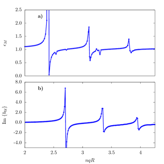
Figure 1: (a) Transverse component $\epsilon_{M}^{T}=\epsilon_{M}^{yy}(\omega,\bm{k})$ of the macroscopic dielectric response of a metamaterial composed of a square lattice of dielectric cylinders of refraction index $n=10$ and radius $R=0.1a$ as a function of the frequency, characterized by $nqR$, for a wavevector along the $x$ direction slightly larger than the vacuum wavevector $k=1.01q$. (b) Sum of the imaginary part of coefficients of the scattered field $\sum_{l}b^{\prime\prime}_{0l}$ of an array of $511\times 511$ dielectic cylinders, obtained from Eq. (32) using a maximum value of $l=1$.

Fig. 1a shows the results for the transverse component of the macroscopic dielectric tensor of the metamaterial $\epsilon_{M}^{T}=\epsilon_{M}^{yy}$ obtained through the recursive numerical approach. The results are shown as a function of the frequency, characterized by the free wavevector within the dielectric normalized to the radius $nqR$. Several resonances are clearly visible. In order to analyze their origin, in Fig. 1b we show the sum of the imaginary part of the scattered field coefficients $\sum_{l}b^{\prime\prime}_{0l}$ obtained from the analytical method. In this calculation we assumed the response of all cylinders was identical, except for the phase factor $\exp(ikX_{n})$ and we included a damping of the cylinder-cylinder interaction at large distances to eliminate the oscillations due to reflections at the edge of the finite array, and thus mimic an infinite array. We checked convergence of this procedure by increasing the number of cylinders.

Three prominent resonant features are observed in both panels of Fig. 1 at low energies. The lowest energy resonance corresponds to a magnetic dipole arising from the term $l=0$, as it lies close to that of an isolated cylinder ocurring at the first zero of the Bessel function around $nqR\approx 2.4$. The second resonance around $nqR\approx\pi$, emerges from the fulfillment of Bragg’s diffraction condition for $2a=2\pi/q$. A third resonance close to $nqR\approx 3.8$ is originated by the term $l=1$. This resonance is strongly enhanced through the interaction between cylinders. The additional peaks in the macroscopic response are due to resonances caused by multiple reflections in the intesrstitial regions. We have verified that they are not due to numerical noise, but they dissapear when a very small artificial dissipation is added to the interstitial dielectric function, while the large peaks are robust. Notice however that the scattering coefficients $b_{0l}$ resonate at higher energies than the macroscopic dielectric function. The reason for this discrepancy is that the transverse normal modes of the system are not actually given by the poles of the dielectric response, but by the poles of the electromagnetic Green’s function.

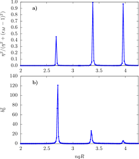
Figure 2: a) Normalized imaginary part of the electromagnetic Green’s function $\eta^{2}/(\eta^{2}+(\epsilon_{T}-k^{2}/q^{2})^{2})$ for a small dissipation parameter $\eta$ as a function of $nqR$ for $k\approx q$ for the same system as in Fig. 1. b) Squared magnitude of the scattering amplitude $b_{0}=\sum_{l}b_{0l}$ for the same system as in Fig. 1.

Figure 2 a) shows the imaginary part of the electromagnetic Green’s function $(\epsilon_{T}-k^{2}/q^{2})^{-1}$ for a small broadening parameter $\eta=0.001$ and b) the squared magnitude of the scattering amplitude $b_{0}=\sum_{l}b_{0l}$ for $k\approx q$ as a function of $nqR$. Here, the peaks of the Green’s function coincide with the peaks of the scattering coefficient as the poles of the Green’s function and of the scattered coefficient correspond both to the normal modes of the system, for which one may have a finite field, and finite scattered amplitudes without an external excitation.

Having verified the consistency of both computational approaches when applied to the calculation of the normal modes of a system, we now consider a more interesting and realistic case. We consider a metamaterial composed of strongly interacting cylinders with a larger radius $R=0.35a$ and a large but realistic refraction index $n=4$ (similar to that of Si). In order to identify exotic behavior such as negative refraction, we have to examine the dispersion relation of the normal modes of the system and explore their group velocity [20, 25]. Thus, we calculated the macroscopic dielectric function and obtained the Green’s function of the metamaterial as a function of both frecuency $\omega$ and wavevector $k$.

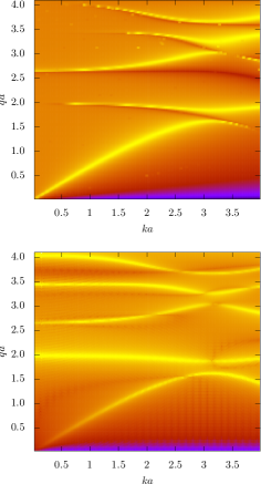
Figure 3: Imaginary part of the Green’s function $(\epsilon_{T}-k^{2}/q^{2})^{-1}$ for a system composed by dielectic cylinders of radius $r=0.35a$ and refractive index $n=4$, obtained numerically through the macroscopic response using the package Photonic (upper panel). Magnitude of the scattered amplitude $b_{0}$ normalized as $\eta/(\eta^{2}+1/b_{0}^{2})$ using a dissipation factor $\eta$ for an array of $201\times 201$ cylinders, obtained through the scattering approach (Eq. (32)) using a maximum value of $l=2$ (lower panel). Color map is logarithmic.

For the numerical calculations we used a two dimensional $201\times 201$ grid and $300$ sets of Haydock coefficients. A very small artificial dissipative term $0.001i$ has been added to the vaccum dielectric constant in order to improve convergence. The results are displayed in Fig. 3. The scattering amplitude obtained from the scattering approach, calculated for an array of $201\times 201$ cylinders considering a maximum value of the orbital number $l=2$ is shown for comparisson.

The upper panel of Fig. 3 shows the imaginary part of the of the Green’s function $\eta/(\eta^{2}+(\epsilon_{M}^{T}-k^{2}/q^{2}))$ where $\epsilon_{M}^{T}$ was obtained numerically through Haydock’s recursion and the results have been smoothed with a dissipation factor $\eta=0.2$ for better visualization. The lower panel shows the absolute value squared of the scattering amplitude $b_{0}=\sum_{l}b_{0l}$, smoothed as $\eta/(\eta^{2}+1/|b_{0}|^{2})$ with a dissipation factor $\eta=0.1$.

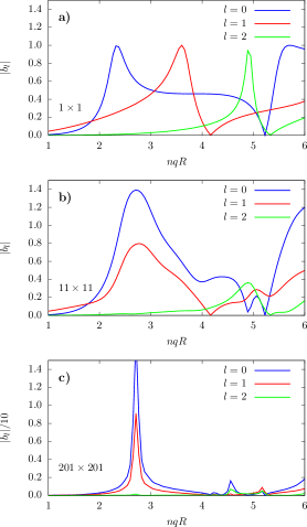
Figure 4: Absolute value of the scattering coefficients $|b_{0l}|$ for an a) isolated cylinder, b) array of $11\times 11$ cylinders and c) array of $201\times 201$ cylinders, as a function of $nqR$.

Several bands may be identified in Fig. 3 showing a very good agreement between the dispersion relations obtained through our two approaches. Regions of negative dispersion, i.e., for which the frequency of the resonances decreases as the wavevector increases, yielding a negative group velocity, are clearly observed for the second, fourth and fifth bands and for large wavevectors before the first Brillouin zone boundary at $ka=\pi$. The bands originate from the combination of isolated cylinder resonances of different values of $l$, while different values of $l$ participate in each band due to the relatively strong interaction between neighboring thick cylinders. This can be confirmed through Figure 4, which shows the absolute value of the individual scattering coefficients $b_{0l}$ for $l=0,1,2$ as a function of $nqR$ for a) a single cylinder, b) an array of $11\times 11$ cylinders and c) an array of $201\times 201$, for a wavevector $k=q$. The coefficients corresponding to an isolated cylinder display one broad peak each around $q=2.4$, $4.8$ and $5.1$ for $l=0,1,2$ respectively, which are close to the first zeroes of the corresponding Bessel function. For an array of $11\times 11$ cylinders these peaks appear distorted and shifted to be finally merged for a larger array of $201\times 201$ in which case all $l$-contributions resonate at the same frequencies.

4 Conclusions

We presented two schemes to calculate the electromagnetic properties of a metamaterial made of a simple lattice of cylinders: a numerical method based on a recursive calculation of the macroscopic dielectric tensor which may be easily generalizable to arbitrary geometries and materials, and a multiple scattering approach for cylindrical geometries which allowed us a simple interpretation of the results in terms of the excitation of Mie resonances. We applied these methods to investigate the response of a system made up of cylinders of high index of refraction. The comparison between the results of both methods is not direct, as in one case we obtain a macroscopic response and in the other we obtain scattering amplitudes. Nevertheless, we showed that the poles of the macroscopic Green’s function obtained by our numerical method coincide with those of the scattering coefficients, and both can be interpreted as the excitation of the normal modes of the system. For a system of thin cylinders with very high index of refraction and a relatively small coupling, we identified the nature of each mode. We found modes arising from the Mie resonances of individual cylinders and a mode arising from Bragg coherent multiple scattering. For larger cylinders the interaction yields a coupling between resonances with different angular momenta. By varying the frequency and wavevector independently we computed the dispersion relation of the normal modes. The photonic band structure obtained using both methods is in very good agreement, and reveal regions of negative dispersion. Thus, through comparison with an ad-hoc model we showed that our macroscopic approach based on Haydock’s recursion and its implementation in the Photonic package is an efficient procedure for obtaining the optical properties of metamaterials made up of high index of refraction cylinders incorporating resonances which cannot be explored within the long wavelength limit. Furthermore, as it can be readily generalized to arbitrary geometries and materials, we believe it will prove to be a useful tool for the design of artificial materials with a richer geometry that might yield novel properties.

This work has been supported by CONACyT through a postdoctoral research fellowship. WLM acknowledges the support from DGAPA-UNAM through grant IN111119. BSM acknowledges the support from CONACYT through grant A1-S-9410.

References

- [1] R. A. Shelby, D. R. Smith, and S. Schultz, Science 292(5514), 77–79 (2001).
- [2] D. R. Smith, J. B. Pendry, and M. C. Wiltshire, Science 305(5685), 788–792 (2004).
- [3] K. Aydin, I. Bulu, K. Guven, M. Kafesaki, C. M. Soukoulis, and E. Ozbay, New Journal of Physics 7(1), 168 (2005).
- [4] A. J. Hoffman, L. Alekseyev, S. S. Howard, K. J. Franz, D. Wasserman, V. A. Podolskiy, E. E. Narimanov, D. L. Sivco, and C. Gmachl, Nature materials 6(12), 946 (2007).
- [5] L. Peng, L. Ran, H. Chen, H. Zhang, J. A. Kong, and T. M. Grzegorczyk, Physical Review Letters 98(15), 157403 (2007).
- [6] A. I. Kuznetsov, A. E. Miroshnichenko, M. L. Brongersma, Y. S. Kivshar, and B. Luk’yanchuk, Science 354(6314), aag2472 (2016).
- [7] S. Linden, C. Enkrich, M. Wegener, J. Zhou, T. Koschny, and C. M. Soukoulis, Science 306(5700), 1351–1353 (2004).
- [8] T. J. Yen, W. J. Padilla, N. Fang, D. C. Vier, D. R. Smith, J. B. Pendry, D. N. Basov, and X. Zhang, Science 303(5663), 1494–1496 (2004).
- [9] Q. Zhao, J. Zhou, F. Zhang, and D. Lippens, Materials Today 12(12), 60 – 69 (2009).
- [10] Y. Kivshar and A. Miroshnichenko, Opt. Photon. News 28(1), 24–31 (2017).
- [11] S. Kruk and Y. Kivshar, ACS Photonics 4(11), 2638–2649 (2017).
- [12] K. Vynck, D. Felbacq, E. Centeno, A. I. Căbuz, D. Cassagne, and B. Guizal, Physical Review Letters 102(Mar), 133901 (2009).
- [13] J. A. Schuller, R. Zia, T. Taubner, and M. L. Brongersma, Physical Review Letters 99(10), 107401 (2007).
- [14] S. Jahani and Z. Jacob, Nature nanotechnology 11(1), 23 (2016).
- [15] C. Zhang, Y. Xu, J. Liu, J. Li, J. Xiang, H. Li, J. Li, Q. Dai, S. Lan, and A. Miroshnichenko, Lighting up silicon nanoparticles with mie resonances, 2018.
- [16] D. Felbacq, G. Tayeb, and D. Maystre, Journal of the Optical Society of America A 11(9), 2526–2538 (1994).
- [17] W. L. Mochán, G. P. Ortiz, and B. S. Mendoza, Optics express 18(21), 22119–22127 (2010).
- [18] U. R. Meza, B. S. Mendoza, and W. L. Mochán, Physical Review B 99(12), 125408 (2019).
- [19] J. S. Pérez-Huerta, G. P. Ortiz, B. S. Mendoza, and W. L. Mochán, New Journal of Physics 15(4), 043037 (2013).
- [20] V. M. Agranovich and Y. N. Gartstein, Physics-Uspekhi 49(10), 1029 (2006).
- [21] R. Haydock, Computer Physics Communications 20(1), 11–16 (1980).
- [22] L. Juárez-Reyes and W. L. Mochán, Physica Status Solidi (b) 255(4), 1700495 (2018).
- [23] D. Gagnon and L. J. Dubé, Journal of Optics 17(10), 103501 (2015).
- [24] W. L. Mochán, G. Ortiz, B. S. Mendoza, and J. S. Pérez-Huerta, Photonic, Comprehensive Perl Archive Network (CPAN), 2016, Perl package for calculations on metamaterials and photonic structures.
- [25] V. Agranovich and Y. N. Gartstein, Metamaterials 3(1), 1–9 (2009).