Recursive Calculation of the Optical Response of Multicomponent Metamaterials

Abstract

We develop a recursive computational procedure to efficiently calculate the macroscopic dielectric function of multi-component metamaterials of arbitrary geometry and composition within the long wavelength approximation. Although the microscopic response of the system might correspond to non-Hermitian operators, we develop a representation of the microscopic fields and of the response, and we introduce an appropriate metric that makes all operators symmetric. This allows us to use a modified Haydock recursion, introducing complex Haydock coefficients that allow an efficient computation of the macroscopic response and the microscopic fields. We test our procedure comparing our results to analytical ones in simple systems, and verifying they obey a generalized multicomponent Keller’ theorem and the Mortola and Stefé’s theorem for four component metalic and dielectric systems.

1 Introduction

Metamaterials made up of a repeated pattern of one or more ordinary materials within a host have optical properties that might differ substantially from those of its components [1]. According to their geometry and composition they might display both electric and magnetic resonances of dipolar and quadrupolar nature [2] around which their macroscopic permittivity and permeability may become negative, yielding an exotic negative refraction [3, 4, 5, 6, 7]. A usual typical geometry of these left-handed and other exotic metamaterials is that of pairs of wires and split conducting rings within a dielectric. Nevertheless, to avoid the dissipation inherent within the conducting phases, all-dielectric structures employing high index of refraction have also been investigated [8, 9], and it has been shown that their Mie like resonances may also be employed for guiding light and for enhancing non-linear optical effects. All dielectric structures of appropriate shapes may also exhibit negative dispersion [10].

The microscopic field within metamaterials may have small regions where the field is very high. Small modifications of the composition at these regions may produce notable macroscopic effects. Thus, metamaterials have been used to develop different kinds of sensors for different spectral regions [11, 12, 13, 14]. Many other known and emerging applications of metamaterials have been reviewed recently [15, 16].

The permeability and permittivity, as well as chiral properties of a metamaterial may be obtained from its reflection and transmission properties [17] and from the dispersion of guided modes within metamaterial waveguides [18], but more fundamentally, from the frequency and wavevector dependence of an appropriately defined spatially-dispersive macroscopic dielectric function [19, 20, 21, 22, 23, 24].

A very efficient scheme for the calculation of the optical properties of metamaterials has been developed for binary metamaterials by exploiting an analogy between the macroscopic dielectric tensor and the projected Green’s function corresponding to a Hermitian Hamiltonian [25] which may be obtained through Haydock’s recursive procedure [26, 27, 28]. The method has been used to study extraordinary transmission through perforated metallic slabs [25], to calculate plasmonic properties of odd shaped metallic inclusions [29], to study enhanced birrefrigency and dichroism in anisotropic metamaterials [30], for the design and optimization of optical devices to control the absorption [31] and polarization of light [32], and to optimize electrical and optical properties of semitransparent contacts [33]. The method has also been generalized to account for retardation, yielding a non-local macroscopic response from which the complete band structure of photonic crystals may be obtained [34] and from which magnetic properties may be extracted [35].

There has also surged interest in the nonlinear properties of metamaterials [36, 37] and metasurfaces [37]. The Haydock’s recursive approach has been extended to calculate the microscopic field and from it the macroscopic non-linear optical response of metamaterials. In particular, to obtain the second harmonic generation spectra of metamaterials with centrosymmetric components but noncentrosymmetric shapes [38].

Unfortunately, the efficient computational approach developed in [25] is directly applicable only to binary metamaterials, that is, to systems composed of exactly two different materials $A$ and $B$. The reason for this limitation is that the geometry of such systems may be decoupled from their composition and described by a characteristic function $B(\bm{r})$ whose value is 1 for those points $\bm{r}$ that belong to region $B$, and 0 when $\bm{r}$ does not, i.e., within region $A$. It is from this characteristic function that a Hermitian operator is built, regardless of the actual composition of $A$ and $B$, and of their dielectric or conducting nature, their dispersion and dissipation. The Haydock coefficients for this operator are readily obtained and from them a closed expression for its macroscopic response may be built. However, for multicomponent systems, one cannot find such a Hermitian operator to describe the geometry, and the dielectric response itself is not Hermitian in the presence of dissipation. Given this limitation, many interesting systems seem to lie beyond the possibilities of the recursive approach. For example, metasurfaces are arrangements of patterned particles on a substrate [39] that have been used to manipulate the refraction of light [40] and produce flat lenses [41], compound lenses [41] and even fabricate spin switchable holograms [42]. A numerical study of metasurfaces would require at least three materials corresponding to the particles, the substrate and the ambient. Similarly, it has been shown that the field enhancement due to resonant excitation of plasmonic particles may not decrease when protected by a dielectric, if the dielectric presents a coexisting Mie resonance [43]. Arrays of metallic cores coated by semiconductors may also display negative index of refraction as an electric dipole plasmonic resonance might coexist with a magnetic dipole Mie resonance [44, 45, 46]. The study of these coupled plasmonic-Mie resonances requires accounting at least for a core, a coating and the ambient.

The purpose of the present paper is to generalize the efficient homogenization procedure using Haydock’s recursion, as presented in Ref. [25], in order to deal with periodic metamaterials of arbitrary geometry and composition and with an arbitrary number of components, or even with a dielectric response that varies continuously in space. To that end, we realize that though the dielectric response is not in general an Hermitian operator, it corresponds to a symmetrical complex operator. Thus, we can cautiously employ well know theorems of linear algebra provided we define an appropriate Euclidean-like metric instead of the usual Hermitian metric. However, this metric couples Bloch waves moving in opposite directions, requiring us to introduce a spinor-like two-component representation of the Bloch states, with one component for each of the opposing propagation directions. Besides obtaining the macroscopic dielectric response of the system, we can also calculate the microscopic electric field, so our procedure can further be employed in non-linear calculations. We restrict ourselves to the non-retarded, long-wavelength approximation, though the same ideas can be applied to fully retarded calculations.

In order to verify the suitability of our computational procedure, we calculate the macroscopic response of various 2D multicomponent systems and verify that our results are consistent with a generalized [47] Keller’s theorem [48], and with Mortola and Steffé’s exact expression [49, 50] for four-component chess-board systems.

The structure of the paper is the following. In Sec. 2 we present our theory: In Subsec. 2.1 we develop our recursive approach to the calculation of the dielectric function. In order to test our results, in Subsec. 2.2 we obtain analytical approximate formulae for the response of a simple multicomponent system, in Subsec. 2.3 we present a generalized Keller’s theorem for multicomponent 2D systems and in Subsec. 2.4 we discuss a 2D four component system for which exact analytical expressions are available. In Sec. 3 we present numerical results for a variety of 2D systems and verify that they agree with analytical results in the appropriate limits, that in general they obey Keller’s theorem and that they are consistent with Mortola and Steffe’s expression. Finally, Sec. 4 is devoted to conclusions.

2 Theory

2.1 Multicomponent metamaterials

In the non-retarded, long-wavelength limit, the longitudinal projection of the macroscopic dielectric function of a periodic system may be obtained from [51, 52]

$$(\hat{\epsilon}_{M}^{LL})^{-1}=(\hat{\epsilon}^{LL})^{-1}_{aa},$$ (1)

where the superscript $LL$ and the subscript $aa$ on an operator $\hat{\mathcal{O}}$ denote the application of longitudinal projectors $\hat{\mathcal{P}}^{L}$ and the application of spatial average projectors $\hat{\mathcal{P}}_{a}$ on both sides of $\hat{\mathcal{O}}$. For a periodic system with its fields represented in reciprocal space we may express the longitudinal and average projectors by the matrices

$$\mathcal{P}^{L}_{\bm{G}\bm{G}^{\prime}}=\hat{\bm{G}}_{\bm{k}}\hat{\bm{G}}_{\bm{k}}\delta_{\bm{G}\bm{G}^{\prime}},$$ (2)

and

$$\mathcal{P}^{a}_{\bm{G}\bm{G}^{\prime}}=\delta_{\bm{G}\bm{0}}\delta_{\bm{G}^{\prime}\bm{0}},$$ (3)

where $\{\bm{G}\}$ is the reciprocal lattice and we abbreviate the unit vectors,

$$\hat{\bm{G}}_{\bm{k}}\equiv\frac{\bm{k}+\bm{G}}{|\bm{k}+\bm{G}|}$$ (4)

where $\bm{k}$ is a small Bloch’s wavevector which in the long-wavelength approximation is assumed to be much smaller that $G$, except for the case $\bm{G}=0$, for which we define the direction $\hat{\bm{0}}_{\bm{k}}\equiv\hat{\bm{k}}/k$. We remark that we may simplify our calculations by reinterpreting the $LL$ projection in Eq. (1) and similar equations below by the $LL$ component, representing any operator $\hat{\mathcal{O}}^{LL}$ by the matrix $\hat{\bm{G}}_{\bm{k}}\cdot\mathcal{O}_{\bm{G}\bm{G}^{\prime}}\hat{\bm{G}}^{\prime}_{\bm{k}}$.

For a system with only two components $A$ and $B$ we define a characteristic function $B(\bm{r})$ which takes the values 0 when $\bm{r}\in A$ and 1 when $\bm{r}\in B$. In this case, we may write the microscopic dielectric function

$$\epsilon(\bm{r})=\frac{\epsilon_{A}}{u}(u-B(\bm{r})),$$ (5)

where $\epsilon_{\alpha}$ is the dielectric function of component $\alpha=A,B$ and

$$u=\frac{1}{1-\epsilon_{B}/\epsilon_{A}},$$ (6)

is the spectral variable. From Eqs. (1) and (5) it is clear that we only need the average projection of the operator

$$\hat{\mathcal{G}}(u)=(u-\hat{B}^{LL})^{-1},$$ (7)

which plays the role of a Green’s function for the operator $\hat{B}^{LL}$, the longitudinal projection of the charateristic function. The spectral variable $u$ would then play the role of a complex energy which depends on the dielectric functions of both media, which in turn are generally complex valued functions of the frequency. As $\hat{B}^{LL}$ is a Hermitian operator, it can be represented as a tridiagonal real matrix with diagonal elements $a_{n}$, and subdiagonal and supradiagonal elements $b_{n}$, its Haydock coefficients, in a basis of Haydock states $\ket{n}$ obtained from an initial macroscopic state $\ket{0}$ by repeatedly applying $\hat{B}^{LL}$ and orthonormalizing the resulting state, i.e., defining

$$\hat{B}^{LL}\ket{n}\equiv b_{n+1}\ket{n+1}+a_{n}\ket{n}+b_{n}\ket{n-1},$$ (8)

with the condition

$$\braket{n}{m}=\delta_{nm}.$$ (9)

The resulting response is given by the continued fraction

$$\epsilon_{M}^{LL}=\frac{\epsilon_{A}}{u}\left(u-a_{0}-\frac{b_{1}^{2}}{u-a_{1}-\frac{b_{2}^{2}}{u-a_{2}-\frac{b_{3}^{2}}{\ddots}}}\right).$$ (10)

Details of this procedure may be seen in Ref. [25].

For multicomponent metamaterials the procedure above does not work, as the geometry of the system would no longer be described by a single characteristic function, and if we introduce several characteristic functions, one for each component, then it wouldn’t be possible to represent all of them by tridiagonal matrices in the same basis. One way out of this difficulty is to use the longitudinal part of the microscopic dielectric function $\hat{\epsilon}^{LL}$ as the operator to use in Haydock’s recursion. If we replace the recursion (8) by

$$\hat{\epsilon}^{LL}\ket{n}\equiv b_{n+1}\ket{n+1}+a_{n}\ket{n}+b_{n}\ket{n-1},\quad\text{(ND)}$$ (11)

then the macroscopic response would be given by

$$\epsilon_{M}^{LL}=\left(a_{0}-\frac{b_{1}^{2}}{a_{1}-\frac{b_{2}^{2}}{a_{2}-\frac{b_{3}^{2}}{\ddots}}}\right).\quad\text{(ND)}$$ (12)

Nevertheless, this procedure would only work in the absence of dissipation, when $\epsilon(\bm{r})$ is real and $\hat{\epsilon}^{LL}$ is a Hermitian operator. Otherwise, there would be no reason for Eq. (11) to contain only three terms on its RHS with real coefficients nor for its first and third terms to contain coefficients from the same set $\{b_{n}\}$. We would have instead

$$\begin{split}\hat{\epsilon}^{LL}\ket{n}\equiv&b_{n+1}\ket{n+1}+a_{n}\ket{n}+c_{n}\ket{n-1}\\ &+d_{n}\ket{n-2}+\ldots\end{split}$$ (13)

with complex coefficients $a_{n}$, $b_{n}$, $c_{n}$, $d_{n}$…, and Eq. (12) would no longer hold. For this reason we flagged Eq. (11) and (12) with ND (no dissipation).

We notice that even when there is dissipation, the longitudinal dielectric function is a symmetrical operator. To show this, we chose an Euclidean scalar product between states

$$\braket{\phi}{\psi}\equiv\int d^{3}\bm{r}\,\phi(\bm{r})\psi(\bm{r})$$ (14)

where $\phi(\bm{r})$ and $\psi(\bm{r})$ are the wavefunctions that represent the states $\ket{\phi}$ and $\ket{\psi}$ in real space. Notice that in Eq. (14) we didn’t conjugate $\phi(\bm{r})$ as we would have done had we chosen a Hermitian product. We can express this scalar product in reciprocal space as

$$\braket{\phi}{\psi}\equiv\int\frac{d^{3}\bm{q}}{(2\pi)^{3}}\phi(-\bm{q})\psi(\bm{q})=\int\frac{d^{3}\bm{q}}{(2\pi)^{3}}\phi(\bm{q})\psi(-\bm{q}),$$ (15)

where we define the Fourier transform $\zeta(\bm{q})$ of any function $\zeta(\bm{r})$ through

$$\zeta(\bm{r})\equiv\int\frac{d^{3}\bm{q}}{(2\pi)^{3}}\zeta(\bm{q})e^{i\bm{q}\cdot\bm{r}}.$$ (16)

Notice in Eq. (15) the minus sign in the argument of $\phi$ instead of the its conjugate as in Parseval’s theorem. Then, we may compute a matrix element of $\hat{\epsilon}^{LL}$ as

$$\braket{\phi}{\hat{\epsilon}^{LL}}{\psi}=-\int\frac{d^{3}\bm{q}}{(2\pi)^{3}}\int\frac{d^{3}\bm{q}^{\prime}}{(2\pi)^{3}}\phi(\bm{q})\hat{\bm{q}}\cdot\epsilon(-\bm{q}-\bm{q}^{\prime})\hat{\bm{q}}\psi(\bm{q}),$$ (17)

where $\epsilon(\bm{q})$ is the Fourier transform of $\epsilon(\bm{r})$. Clearly, $\braket{\phi}{\hat{\epsilon}^{LL}}{\psi}=\braket{\psi}{\hat{\epsilon}^{LL}}{\phi}$ showing that the operator $\hat{\epsilon}^{LL}$ is symmetric under the appropriate scalar product.

Notice that for a periodic system, $\epsilon(\bm{r})=\epsilon(\bm{r}+\bm{R})$ may be written as a Fourier series with coefficients

$$\epsilon_{\bm{G}}=\int_{\text{UC}}\frac{d^{3}r}{\Omega}\epsilon(\bm{r})e^{-i\bm{G}\cdot\bm{r}},$$ (18)

related to the Fourier transform $\epsilon(\bm{q})=(2\pi)^{3}\sum_{\bm{G}}\epsilon_{\bm{G}}\delta(\bm{q}-\bm{G})$, where $\{\bm{R}\}$ is the Bravais lattice, $\{\bm{G}\}$ its reciprocal lattice, and UC indicates that the integral is over a unit cell, whose volume is $\Omega$. Thus, we can write Eq. (17) as

$$\begin{split}\braket{\phi}{\hat{\epsilon}^{LL}}{\psi}=&\int_{\text{BZ}}\frac{d^{3}\bm{k}}{(2\pi)^{3}}\sum_{\bm{G}}\sum_{\bm{G}^{\prime}}\phi(-\bm{k}-\bm{G})\\ &\hat{\bm{G}}\cdot\epsilon_{\bm{G}-\bm{G}^{\prime}}\hat{\bm{G}^{\prime}}\psi(\bm{k}+\bm{G}^{\prime}),\end{split}$$ (19)

where we replaced the wavevector $\bm{q}$ by the sum of a Bloch’s vector $\bm{k}$ and some reciprocal vector $\bm{G}$, and BZ indicates that the integral is over the first Brillouin zone. Ordinarily, in a periodic system, the normal modes of the system may be chosen as Bloch waves with a single Bloch’s vector $\bm{k}$. However, our chosen metric couples $\bm{k}$ to $-\bm{k}$. Thus we will consider simultaneously states with given Bloch’s vectors $\pm\bm{k}$ and denote them using a spinor-like notation as,

$$\ket{\zeta}\to\left(\begin{array}[]{c}\zeta(\bm{k}+\bm{G})\\ \zeta(-\bm{k}+\bm{G})\end{array}\right).$$ (20)

Consequently, we represent the dielectric response as a $2\times 2$ matrix,

$$\hat{\epsilon}^{LL}\to\left(\begin{array}[]{cc}\hat{\bm{G}}_{\bm{k}}\cdot\epsilon_{\bm{G}-\bm{G}^{\prime}}\hat{\bm{G}^{\prime}}_{\bm{k}}&0\\ 0&\hat{\bm{G}}_{-\bm{k}}\cdot\epsilon_{\bm{G}-\bm{G}^{\prime}}\hat{\bm{G}^{\prime}}_{-\bm{k}}\end{array}\right).$$ (21)

The scalar product (15) becomes

$$\begin{split}\braket{\phi}{\psi}=\sum_{G}&\left(\phi(-\bm{k}-\bm{G})\psi(\bm{k}+\bm{G})\right.\\ &+\left.\phi(\bm{k}-\bm{G})\psi(-\bm{k}+\bm{G})\right).\end{split}$$ (22)

From Eqs. (20)–(22) we get

$$\begin{split}\braket{\phi}{\hat{\epsilon}^{LL}}{\psi}&=\sum_{\bm{G}\bm{G}^{\prime}}\left(\phi(-\bm{k}-\bm{G})\hat{\bm{G}}_{\bm{k}}\cdot\epsilon_{\bm{G}-\bm{G}^{\prime}}\hat{\bm{G}^{\prime}}_{\bm{k}}\psi(\bm{k}+\bm{G}^{\prime})\right.\\ &+\left.\phi(\bm{k}-\bm{G})\hat{\bm{G}}_{-\bm{k}}\cdot\epsilon_{\bm{G}-\bm{G}^{\prime}}\hat{\bm{G}^{\prime}}_{-\bm{k}}\psi(-\bm{k}+\bm{G}^{\prime})\right).\end{split}$$ (23)

Using Eqs. (20)–(23) we can proceed to build a Haydock’s representation of the operator $\hat{\epsilon}^{LL}$. We start from a couple of macroscopic states representing longitudinal waves propagating in the directions $\pm\hat{\bm{k}}$, corresponding to the starting spinor

$$\ket{0}\to\frac{1}{\sqrt{2}}\left(\begin{array}[]{c}1\\ 1\end{array}\right)\delta_{\bm{G}\bm{0}},$$ (24)

normalized according to Eq. (22). We also define a state $\ket{-1}\to 0$. Then we repeatedly apply $\hat{\epsilon}^{LL}$ using the matrix representation (21) and we orthonormalize the resulting states to the previously obtained states, through Haydock’s recursion

$$b_{n+1}\ket{n+1}=\hat{\epsilon}^{LL}\ket{n}-a_{n}\ket{n}-b_{n}\ket{n-1},$$ (25)

where we demand

$$\braket{n}{m}=\delta_{nm}$$ (26)

using the product (22). Thus,

$$a_{n}=\braket{n}{\hat{\epsilon}^{LL}}{n}$$ (27)

and

$$\begin{split}b_{n+1}^{2}=&(\bra{n}\hat{\epsilon}^{LL}-a_{n}\bra{n}-b_{n}\bra{n-1})\\ &(\hat{\epsilon}^{LL}\ket{n}-a_{n}\ket{n}-b_{n}\ket{n-1}).\end{split}$$ (28)

We remark that the symmetry of $\hat{\epsilon}^{LL}$ guarantees that the coefficient of $\ket{n-1}$ is $b_{n}$, that there are no more terms in Eq. (25) and that the resulting state $\ket{n+1}$ is implicitly orthogonal to all previous states $\ket{0}\ldots\ket{n-1}$ even though we only orthogonalize it explicitly to $\ket{n}$, except for the accumulation of numerical errors, which would have to be handled in the implementation [53, 54, 55]. In analogy to Ref. [25], the products by $\hat{\bm{G}}_{\pm\bm{k}}$ and $\hat{\bm{G}}^{\prime}_{\pm\bm{k}}$ in Eq. (23) may be performed in reciprocal space, while the convolution with $\epsilon_{\bm{G}-\bm{G}^{\prime}}$ may be replaced by a simple multiplication with $\epsilon(\bm{r})$ in real space, so that we may apply the operator $\hat{\epsilon}^{LL}$ without involving any large matrix product. The Haydock coefficients in Eqs. (27) and (28) are not guaranteed to be real and positive as those in Eq. (8) and may be complex valued. As in Ref. [25], in the orthonormal basis $\{\ket{n}\}$ the microscopic longitudinal dielectric function is represented by a tridiagonal symmetric matrix

$$\hat{\epsilon}^{LL}\to T_{nn^{\prime}}=\left(\begin{array}[]{ccccc}a_{0}&b_{1}&0&0&\ldots\\ b_{1}&a_{1}&b_{2}&0&\ldots\\ 0&b_{2}&a_{2}&b_{3}&\ldots\\ \vdots&\vdots&\vdots&\vdots&\ddots\end{array}\right),$$ (29)

from which Eq. (1) allows to extract the macroscopic response

$$\epsilon_{M}^{LL}=\left(a_{0}-\frac{b_{1}^{2}}{a_{1}-\frac{b_{2}^{2}}{a_{2}-\frac{b_{3}^{2}}{\ddots}}}\right).$$ (30)

Notice that Eq. (30) seems identical to (12), but its Haydock coefficients are different, as they are obtained by using spinor-like states and an Euclidean metric. Thus, Eq. (30) may be used for arbitrary compositions, including multiple disperssive and dissipative media or even a continuosly varying complex response $\epsilon(\bm{r})$.

By identifying the longitudinal displacement field $\bm{D}^{L}$ with an external macroscopic field and thus with no spatial fluctuations, we may represent it in Haydock’s basis as a column vector with components $\bm{D}^{L}\to d_{n}=D^{L}\delta_{n0}$. We may expand the longitudinal electric field in the same basis as $\bm{E}^{L}\to e_{n}$, and solve the tridiagonal system

$$\sum_{n^{\prime}}T_{nn^{\prime}}e_{n^{\prime}}=d_{n^{\prime}}$$ (31)

for the unknowns $e_{n}$ to obtain a representation of the microscopic electric field $\bm{E}^{L}\to\sum e_{n}\ket{n}$ which may be translated into reciprocal or real space to obtain $\bm{E}^{L}(\bm{k}+\bm{G})$ or $\bm{E}^{L}(\bm{r})$.

We have implemented the formalism above as a set of modules written in the Perl programming language, using its Perl Data Language (PDL) [56] extension for efficient numerical calculations, and the Moose [57] object system, and we have incorporated them into the publicly available package Photonic [58].

2.2 Coated clylinders

A simple system to test our approach above is that of a lattice of coated cylindrical particles. Consider a single multilayered cylindrical particle with a core ($p=1$) covered by $N-1$ coaxial shells ($p=2\ldots N$) within vacuum ($p=N+1$). Each layer is characterized by an outer radius $a_{p}$ and a dielectric function $\epsilon_{p}$. The system is subject to an external field $\bm{E}_{\text{ex}}=E_{\text{ex}}\hat{x}$. The potential within each layer may be written as

$$\phi_{p}(\bm{r})=(A_{p}r+B_{p}/r)\cos\theta$$ (32)

in polar coordinates, where, using the symmetry of the system, we restricted ourselves to the angular momentum $l=1$ of the external potential. The boundary conditions at the $p$-th boundary may be written as

$$\left(\begin{array}[]{c}A_{p+1}\\ B_{p+1}\end{array}\right)=\mathcal{M}_{p}\left(\begin{array}[]{c}A_{p}\\ B_{p}\end{array}\right),$$ (33)

where we introduced the transfer matrix

$$M_{p}=\frac{1}{2}\left(\begin{array}[]{cc}\frac{\epsilon_{p+1}+\epsilon_{p}}{\epsilon_{p+1}}&\frac{\epsilon_{p+1}-\epsilon_{p}}{a_{p}^{2}\epsilon_{p+1}}\\ \frac{\epsilon_{p+1}-\epsilon_{p}}{\epsilon_{p+1}}a_{p}^{2}&\frac{\epsilon_{p+1}+\epsilon_{p}}{\epsilon_{p+1}}\end{array}\right).$$ (34)

Using Eq. (33) repeatedly, we may relate

$$\left(\begin{array}[]{c}A_{N+1}\\ B_{N+1}\end{array}\right)=\mathcal{M}\left(\begin{array}[]{c}A_{1}\\ B_{1}\end{array}\right),$$ (35)

with $\mathcal{M}=\mathcal{M}_{N}\mathcal{M}_{N-1}\ldots\mathcal{M}_{2}\mathcal{M}_{1}$. As we may identify $A_{N+1}=-E_{\text{ex}}$ and $B_{N+1}=2p$, with $p$ the total dipole moment per unit length, and as $B_{1}=0$ to avoid a singularity at $r=0$, from Eq. (35) we may obtain the polarizability per unit length of the particle

$$\alpha=\frac{p}{E_{\text{ex}}}=-\frac{\mathcal{M}_{21}}{2\mathcal{M}_{11}}.$$ (36)

For a square array of such coated cylinders we may approximate the macroscopic dielectric response through the Claussius-Mossotti 2D relation

$$\epsilon_{M}=\frac{1+2\pi n\alpha}{1-2\pi n\alpha}$$ (37)

where $n$ is the number density. We expect this expression to hold as long as the distance between cylinders is not so short as to allow exciting multipoles higher than the dipole.

2.3 Keller’s theorem

In order to further test our result (30) we will show below that they satisfy a generalization of Keller’s theorem [47] for multicomponent metamaterials, which we prove in a simple (limited) form below. Consider a 2D metamaterial with three or more components $A$, $B$, $C$…, each characterized by a dielectric function $\epsilon_{A}$, $\epsilon_{B}$, $\epsilon_{C}$…Then, we write its dielectric function as

$$\epsilon\equiv\epsilon(\epsilon_{A},\epsilon_{B},\epsilon_{C},\ldots)=\epsilon_{A}A+\epsilon_{B}B+\epsilon_{C}C+\ldots,$$ (38)

where we introduced characteristic functions $A(\bm{r})$, $B(\bm{r})$, $C(\bm{r})$…, that take the value 1 when $\bm{r}$ lies within the corresponding region $A$, $B$, $C$…and 0 otherwise. We expect the use of the same letters to denote materials, regions and characteristic functions will not be confusing, as their use may be distinguished by context. In the absence of external charge and neglecting retardation, the microscopic displacement and electric fields are solenoidal and irrotational respectively,

$$\begin{array}[]{cc}\nabla\cdot\bm{D}=0,&\nabla\times\bm{E}=0,\end{array}$$ (39)

and they are related through

$$\bm{D}=\epsilon(\epsilon_{A},\epsilon_{B},\epsilon_{C}\ldots)\bm{E}=\epsilon\bm{E}.$$ (40)

Now consider the rotated fields $\bm{D}^{R}(\bm{r})\equiv\mathcal{R}\bm{D}(\bm{r})$ and $\bm{E}^{R}(\bm{r})\equiv\mathcal{R}\bm{E}(\bm{r})$, where

$$\mathcal{R}\equiv\left(\begin{array}[]{cc}0&1\\ -1&0\end{array}\right)$$ (41)

is a rotation matrix by $\pi/2$. Notice that we rotate the fields but not their application point $\bm{r}$. As $\mathcal{R}$ coincides with the Levi-Civita symbol in 2D, then

$$\begin{array}[]{cc}\nabla\cdot\bm{E}^{R}=0,&\nabla\times\bm{D}^{R}=0,\end{array}$$ (42)

which are similar to Eqs. (39) but with the substitutions

$$\begin{array}[]{cc}\bm{D}\to\tilde{\bm{D}}\equiv\bm{E}^{R},&\bm{E}\to\tilde{\bm{E}}\equiv\bm{D}^{R}.\end{array}$$ (43)

Notice that

$$\tilde{\bm{D}}=\epsilon(1/\epsilon_{A},1/\epsilon_{B},1/\epsilon_{C}\ldots)\tilde{\bm{E}}\equiv\tilde{\epsilon}\tilde{\bm{E}}.$$ (44)

Thus, $\tilde{\bm{D}}$ and $\tilde{\bm{E}}$ obey the same equations as $\bm{D}$ and $\bm{E}$ but they are related through a microscopic dielectric response $\tilde{\epsilon}$ identical to that in Eq. (38) but for the replacements $\epsilon_{A}\to 1/\epsilon_{A}$, $\epsilon_{B}\to 1/\epsilon_{B}$, $\epsilon_{C}\to 1/\epsilon_{C}$…

Through a homogenization procedure, such as using Eq. (1), from Eqs. (40) and (44) we obtain $\bm{D}_{M}=\bm{\epsilon}_{M}\bm{E}_{M}$ and $\tilde{\bm{D}}_{M}=\tilde{\bm{\epsilon}}_{M}\tilde{\bm{E}}_{M}$, where $\bm{\epsilon}_{M}$ is the macroscopic dielectric tensor of the original system and $\tilde{\bm{\epsilon}}_{M}$ is the corresponding response of the system obtained from the original one by replacing the response of each component by its inverse. Then we may write

$$\begin{split}\bm{E}_{M}=&\mathcal{R}^{-1}\tilde{\bm{D}}_{M}=\mathcal{R}^{-1}\tilde{\bm{\epsilon}}_{M}\tilde{\bm{E}}_{M}\\ &=\mathcal{R}^{-1}\tilde{\bm{\epsilon}}_{M}\mathcal{R}{\bm{D}_{M}}=\mathcal{R}^{-1}\tilde{\bm{\epsilon}}_{M}\mathcal{R}\bm{\epsilon}_{M}{\bm{E}_{M}},\end{split}$$ (45)

and cancelling $\bm{E}_{M}$ we finally obtain

$$\tilde{\bm{\epsilon}}_{M}^{R}\bm{\epsilon}_{M}=\bm{1},$$ (46)

where $\tilde{\bm{\epsilon}}_{M}^{R}=\mathcal{R}^{-1}\tilde{\bm{\epsilon}}_{M}\mathcal{R}$. Thus the original macroscopic response times the rotated macroscopic response of the system with the reciprocal dielectric functions yields the unit tensor. This is Keller’s theorem for multicomponent metamaterials in 2D.

2.4 Mortola and Steffe’s theorem

Consider now a 2D system made of a square lattice whose unit cell is divided into four identical squares that are occupied from left to right, top to bottom, by four materials $A$, $B$, $C$, $D$. Mortola and Steffe proposed an expression [49] for the macroscopic conductivity of this system in terms of the conductivities of its components. This expression was later proved by Milton [50]. However, as argued in [47], we expect that the correct expression for finite frequencies is that written in terms of the dielectric response, i.e.,

$$\begin{split}\epsilon_{M}^{xx}=&\{[(\epsilon_{A}+\epsilon_{C})(\epsilon_{B}+\epsilon_{D})(\epsilon_{A}\epsilon_{B}\epsilon_{C}+\epsilon_{B}\epsilon_{C}\epsilon_{D}\\ &+\epsilon_{C}\epsilon_{D}\epsilon_{A}+\epsilon_{D}\epsilon_{A}\epsilon_{B})]/[(\epsilon_{A}+\epsilon_{B})(\epsilon_{C}+\epsilon_{D})\\ &\times(\epsilon_{A}+\epsilon_{B}+\epsilon_{C}+\epsilon_{D})]\}^{1/2}.\end{split}$$ (47)

A similar expression holds for $\epsilon_{M}^{yy}$ obtained from Eq. (47) by exchanging $B\leftrightarrow C$.

3 Results

In Figure 1 we show the imaginary part of the dielectric function of a square lattice of thin coated and uncoated Ag cylinders of radius $a_{\text{Ag}}=0.1L$ within vacuum, where $L$ is the lattice parameter. As the cylinders are very thin, their mutual interaction is negligible. Thus, in the case of the uncoated cylinders, there is a peak around $\hbar\omega\approx 3.7$eV which corresponds to the surface plasmon of an isolated Ag cylinder, given by $\epsilon_{\text{Ag}}=-1$. If the cylinder is coated by a SiO₂ layer of outer radius $a_{\text{SiO}_{2}}=0.25L$ the peak is redshifted. The analytical result based on the Claussius-Mossotti relation using the polarizability given by Eq. (36) based on a transfer matrix formalism agrees quite closely with the numerical calculation based on Haydock’s recursion for the case of coated cylinders and is indistinguishable for the case of uncoated cylinders. The numerical calculation was done using a $401\times 401$ grid and with up to 200 pairs of Haydock coefficients.

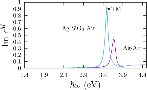
Figure 1: Imaginary part of the macroscopic dielectric function $\epsilon_{M}$ of a square lattice of Ag cylinders of radius $a_{\text{Ag}}=0.1L$ in vacuum, where $L$ is the lattice parameter. One curve corresponds to uncoated cylinders and the other to cylinders coated by a SiO₂ shell with outer radius $a_{\text{SiO}_{2}}=0.25L$. We show results obtained analytically through Eq. (37) and the transfer matrix formalism (TM) and numerically through the procedure developed in Subsec. 2.1.

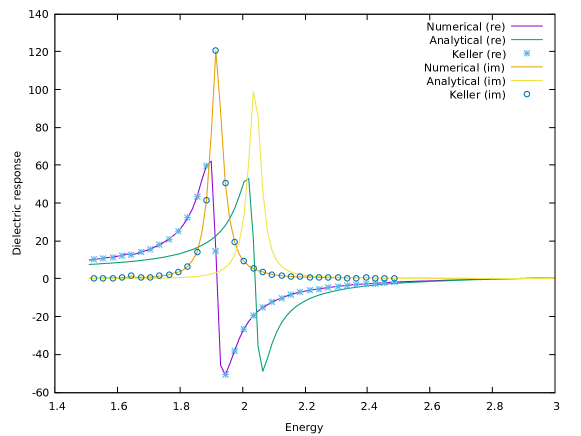
Figure 2: Real and imaginary part of the macroscopic dielectric function $\epsilon_{M}$ of a square lattice of SiO₂ cylinders of radius $a_{\text{SiO}_{2}}=0.3L$ covered by shells of Ag with outer radius $a_{\text{Ag}}=0.45L$, where $L$ is the lattice parameter. We show results obtained analytically and numerically through the procedure developed in Subsec. 2.1. We also show results obtained numerically by applying Keller’s theorem.

Fig. 2 shows the real and imaginary parts of the macroscopic dielectric function for a system similar to that in Fig. 1 but with an SiO₂ core of radius $a_{\text{SiO}_{2}}=0.3L$ covered by an Ag shell of outer radius $a_{\text{Ag}}=0.45L$. As neighboring cylinders are closer together than in Fig. 1 dipolar and higher multipoles may couple together. Thus, the extension (37) of the Claussius-Mossotti formalism may not be accurate. The response obtained from the numerical calculation has a peak around 1.92eV further red-shifted from that of the isolated cylinder than the peak of the analytical calculation around 2.04eV. Nevertheless, a numerical calculation based on Keller’s theorem, Eq. (46), obtained by inverting the dielectric functions of the components, calculating the corresponding dielectric function using our recursive formalism and inverting the result, seems to agree perfectly with the straightforward numerical calculation. Thus, our recursive procedure agrees with Keller’s theorem even for large inclusions and strong interactions.

In Fig. 3 we show the real and imaginary parts of a component $\epsilon_{M}^{xx}$ of the macroscopic dielectric tensor of a metamaterial made up of four materials, Au, Ag, TiO₂ and SiO₂ filling square prisms occupying a 2x2 block and repeated periódically in a checkerboard geometry, as illustrated in Fig. 4. The calculation was performed using the procedure described in Subsec. 2.1 using a $201\times 201$ grid and with up to 300 Haydock coefficient pairs. In the figure we also show the results of an analytical calculation using the formula presented in Subsec. 2.4.

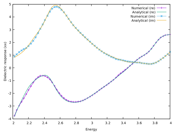
Figure 3: Real and imaginary part of the component $\epsilon_{M}^{xx}$ of the macroscopic dielectric tensor of a four component metamaterial made of square prisms of Au, Ag, TiO₂ and SiO₂ arranged in a square unit cell repeated periodically with the geometry of a checkerboard, as illustrated by Fig. 4, as a function of photon energy $\hbar\omega$. The results obtained numerically using the procedure developed in Subsec. 2.1 are compared to those obtained from the analytical formula presented in Subsec. 2.4

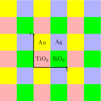
Figure 4: Geometry of the metamaterial corresponding to Fig. 3, consisting of the periodic repetition of a unit cell made up of four square prisms of Au, Ag, TiO₂ and SiO₂.

Notice the good agreement for both the real and imaginary parts for a wide energy range.

4 Conclusions

We have developed a recursive procedure based on a Haydock’s representation that allows the efficient calculation of the macroscopic dielectric function and the microscopic fields of multicomponent metamaterials of arbitrary composition and geometry. Our formalism admits materials that can be insulating, conducting, transparent, opaque, dissipative, and/or dispersive. Although the response of the system may be non-Hermitian, we could take advantage of its symmetric nature by introducing an appropriate scalar product and using a spinor-like representation of the fields. Though efficient, the procedure developed here is not as fast as that for only two materias, as in the current case the Haydock coefficients depend on the composition and not only on the geometry. The results presented here correspond to the non-retarded limit, though we have verified that the same ideas may be extended to the retarded region where they may even be applied to chiral systems. We have prepared computational modules implementing our procedures and added them to a publicly available software package. We tested our formalism by calculating the response of simple systems for which approximate analytical formulae are available, and by demonstrating that our results are consistent with some exact conditions, namely, Keller’s and Mortola and Steffe’s theorems.

This work was supported by DGAPA-UNAM under grant IN111119. RS acknowledges a scholarship from CONACyT.

Graphical Table of Contents

GTOC image:

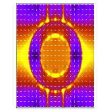
Figure 5: *

We develop an efficient procedure to compute recursively the fields and the response of metamaterials made of any number of components with an arbitrary geometry and composition, metallic or dielectric, transparent or dissipative, using a spinor-like representation of the field states. We test the procedure against systems with analytically determined properties. The figure shows the field of a square array of Ag covered SiO₂ cylinders close to resonance.

References

- [1] V. M. Shalaev, Nat Photon 1(1), 41–48 (2007).
- [2] D. J. Cho, F. Wang, X. Zhang, and Y. R. Shen, Phys. Rev. B 78(12), 121101 (2008).
- [3] R. A. Shelby, D. R. Smith, and S. Schultz, Science 292(5514), 77–79 (2001).
- [4] D. R. Smith, J. B. Pendry, and M. C. Wiltshire, Science 305(5685), 788–792 (2004).
- [5] K. Aydin, I. Bulu, K. Guven, M. Kafesaki, C. M. Soukoulis, and E. Ozbay, New Journal of Physics 7(1), 168 (2005).
- [6] A. J. Hoffman, L. Alekseyev, S. S. Howard, K. J. Franz, D. Wasserman, V. A. Podolskiy, E. E. Narimanov, D. L. Sivco, and C. Gmachl, Nature materials 6(12), 946 (2007).
- [7] L. Peng, L. Ran, H. Chen, H. Zhang, J. A. Kong, and T. M. Grzegorczyk, Physical review letters 98(15), 157403 (2007).
- [8] S. Jahani and Z. Jacob, Nature Nanotechnology 11(1), nnano.2015.304 (2016).
- [9] Y. Kivshar, Natl Sci Rev 5(2), 144–158 (2018).
- [10] K. Vynck, D. Felbacq, E. Centeno, A. I. Căbuz, D. Cassagne, and B. Guizal, Phys. Rev. Lett. 102(13), 133901 (2009).
- [11] Ming Huang and Jingjing Yang, Microwave Sensor Using Metamaterials, in: Wave Propagation, (InTech, March 2011), Dr. Andrei Petrin (Ed.).
- [12] L. La Spada, F. Bilotti, and L. Vegni, Progress In Electromagnetics Research B 34(January) (2011).
- [13] T. Chen, S. Li, and H. Sun, Sensors 12(3), 2742–2765 (2012).
- [14] N. Wongkasem, A. Sonsilphong, and M. Gonzalez, 1 44(3), 178–181 (2017).
- [15] J. Pendry, Nat Mater 5(8), 599–600 (2006).
- [16] A. Baev, P. N. Prasad, H. Ågren, M. Samoć, and M. Wegener, Physics Reports 594(September), 1–60 (2015).
- [17] D. R. Smith, S. Schultz, P. Markoš, and C. M. Soukoulis, Phys. Rev. B 65(19), 195104 (2002).
- [18] H. Chen, J. Zhang, Y. Bai, Y. Luo, L. Ran, Q. Jiang, and J. A. Kong, Opt. Express, OE 14(26), 12944–12949 (2006).
- [19] V. M. Agranovich, Y. R. Shen, R. H. Baughman, and A. A. Zakhidov, Phys. Rev. B 69(16), 165112 (2004).
- [20] M. G. Silveirinha, Phys. Rev. B 75(11), 115104 (2007).
- [21] V. M. Agranovich and Y. N. Gartstein, Metamaterials 3(1), 1–9 (2009).
- [22] A. Alù, Phys. Rev. B 83(8), 081102 (2011).
- [23] A. Alù, Phys. Rev. B 84(7), 075153 (2011).
- [24] A. Konovalenko, J. A. R. Avendaño, A. M. Blas, F. Cervera, E. Myslivets, S. Radic, J. S. D. Moreno, and F. Perez-Rodriguez, J. Opt. (2019).
- [25] W. L. Mochán, G. P. Ortiz, and B. S. Mendoza, Opt. Express, OE 18(21), 22119–22127 (2010).
- [26] R. Haydock, V. Heine, and M. J. Kelly, J. Phys. C: Solid State Phys. 5(20), 2845 (1972).
- [27] R. Haydock, Solid State Physics 35, 215 (1980).
- [28] D. G. Pettifor and D. L. Weaire (eds.), The Recursion Method and Its Applications, Springer Series in Solid State Sciences, Vol. 58 (Springer, Berlin, 1984).
- [29] E. Cortes, L. Mochán, B. S. Mendoza, and G. P. Ortiz, phys. stat. sol. (b) 247(8), 2102–2107 (2010).
- [30] B. S. Mendoza and W. L. Mochán, Phys. Rev. B 85(12), 125418 (2012).
- [31] G. Ortiz, M. Inchaussandague, D. Skigin, R. Depine, and W. L. Mochán, J. Opt. 16(10), 105012 (2014).
- [32] B. S. Mendoza and W. L. Mochán, Phys. Rev. B 94(19), 195137 (2016).
- [33] V. J. Toranzos, G. P. Ortiz, W. L. Mochán, and J. O. Zerbino, Mater. Res. Express 4(1), 015026 (2017).
- [34] J. S. Pérez-Huerta, G. P. Ortiz, B. S. Mendoza, and W. Luis Mochán, New Journal of Physics 15(4), 043037 (2013).
- [35] L. Juárez-Reyes and W. L. Mochán, physica status solidi (b) 255(4), 1700495 (2018).
- [36] M. Lapine, I. V. Shadrivov, and Y. S. Kivshar, Rev. Mod. Phys. 86(3), 1093–1123 (2014).
- [37] R. Czaplicki, J. Mäkitalo, R. Siikanen, H. Husu, J. Lehtolahti, M. Kuittinen, and M. Kauranen, Nano Letters 15(1), 530–534 (2015), PMID: 25521745.
- [38] U. R. Meza, B. S. Mendoza, and W. L. Mochán, Phys. Rev. B 99(12), 125408 (2019).
- [39] N. Yu and F. Capasso, Nature Materials 13(2), 139–150 (2014).
- [40] N. Yu, P. Genevet, M. A. Kats, F. Aieta, J. P. Tetienne, F. Capasso, and Z. Gaburro, Science 334(6054), 333–337 (2011).
- [41] M. Khorasaninejad, W. T. Chen, R. C. Devlin, J. Oh, A. Y. Zhu, and F. Capasso, Science 352(6290), 1190–1194 (2016).
- [42] Y. Chen, X. Yang, and J. Gao, Light Sci Appl 7(1), 1–10 (2018).
- [43] Liren Deng, Yanni Zhai, Yun Chen, Ningning Wang, and Yu Huang, Journal of Physics D: Applied Physics 52(43), 43LT01 (2019).
- [44] R. Paniagua-Domínguez, D. R. Abujetas, and J. A. Sánchez-Gil, Scientific Reports 3(March), 1507 (2013).
- [45] R. Paniagua-Domínguez, F. López-Tejeira, R. Marqués, and J. A. Sánchez-Gil, New J. Phys. 13(12), 123017 (2011).
- [46] D. R. Abujetas, R. Paniagua-Domínguez, M. Nieto-Vesperinas, and J. A. Sánchez-Gil, J. Opt. 17(12), 125104 (2015).
- [47] G. P. Ortiz and W. L. Mochán, New J. Phys. 20(2), 023028 (2018).
- [48] J. B. Keller, Journal of Mathematical Physics 5(4), 548–549 (1964).
- [49] S. Mortola and S. Steffé, Atti Accad. Naz. Lincei, Cl. Sci. Fis., Mat. Nat., Rend. 78, 77 (1985).
- [50] G. W. Milton, Journal of Mathematical Physics 42(10), 4873–4882 (2001).
- [51] W. L. Mochán and R. G. Barrera, Phys. Rev. B 32(8), 4984–4988 (1985).
- [52] W. L. Mochán and R. G. Barrera, Phys. Rev. B 32(8), 4989–5001 (1985).
- [53] H. D. Simon, Linear Algebra and its Applications 61(September), 101–131 (1984).
- [54] Horst D. Simon, Mathematics of Computation 42(165), 115–142 (1984).
- [55] Z. Bai, J. Demmel, J. Dongarra, A. Ruhe, and H. van der Vorst, Lanczos Method, in: Templates for the Solution of Algebraic Eigenvalue Problems: A Practical Guide, (SIAM, Philadelphia, 2000).
- [56] K. Glazebrook and F. Economou, Dr. Dobb’s Journal 22(9) (1997).
- [57] S. Ducasse, M. Lanza, and S. Tichelaar, Moose: An extensible language-independent environment for reengineering object-oriented systems, in: Proceedings of the Second International Symposium on Constructing Software Engineering Tools (CoSET 2000), (IEEE, 2000).
- [58] W. L. Mochán, G. Ortiz, B. S. Mendoza, and J. S. Pérez-Huerta, Photonic, Comprehensive Perl Archive Network (CPAN), 2016, Perl package for calculations on metamaterials and photonic structures.