The complications of learning from Super Soft Source X-ray spectra

Abstract

Super Soft X-ray Sources (SSS) are powered by nuclear burning on the surface of an accreting white dwarf, they are seen around 0.1-1 keV (thus in the soft X-ray regime), depending on effective temperature and the amount of intervening interstellar neutral hydrogen ($N_{\rm H}$). The most realistic model to derive physical parameters from observed SSS spectra would be an atmosphere model that simulates the radiation transport processes. However, observed SSS high-resolution grating spectra reveal highly complex details that cast doubts on the feasibility of achieving unique results from atmosphere modeling. In this article, I discuss two independent atmosphere model analyses of the same data set, leading to different results. I then show some of the details that complicate the analysis and conclude that we need to approach the interpretation of high-resolution SSS spectra differently. We need to focus more on the data than the models and to use more phenomenological approaches as is traditionally done with optical spectra.

1 Introduction

Cataclysmic Variables are characterised by mass transfer from a companion star onto the surface of a white dwarf. If there was only accretion, the white dwarf would grow in mass until reaching the Chandrasekhar mass limit, when it either collapses into a neutron star or explodes as a supernova Ia (if the composition is rich in carbon and oxygen). However, life is more complicated. Since the accreted material is rich in hydrogen, it can fuse to helium, an energy source that leads to mass loss which can be more than the amount of mass gained by accretion. This may happen after a long episode of accretion leading to a successive increase in temperature and pressure. If ignition conditions are reached, the accreted hydrogen explodes in a thermonuclear runaway known as a nova. The radiation pressure drives an initially optically thick wind that obscures any high-energy radiation from the nuclear burning zones. If the mass lost in the wind is higher than the mass previously accreted, then the white dwarf cannot reach the Chandrasekhar mass limit. When the wind becomes optically thin, the central burning regions can be seen. Radiation temperatures then reach several $10^{5}$ K, and a blackbody of this temperature has it’s Wien tail in the soft X-ray regime, around 1 keV ($\sim 10$ Å). A small fraction of white dwarfs permanently host conditions of temperature and pressure to allow the hydrogen-rich accreted material to undergo nuclear fusion at the same rate as the accretion rate. The observational class of these Super Soft Sources (SSS) was discovered by the Einstein satellite and significantly expanded with large-area ROSAT observations. Initially it was believed that they were powered by accretion in neutron stars, but van den Heuvel et al. (1992) proposed nuclear burning on white dwarfs which was later confirmed by Kahabka and van den Heuvel (1997).

In order to see a permanent SSS spectrum, special fine tuning of several parameters such as accretion rate and burning rate is needed, and the class is thus very small. Further, the softness of the spectra allows us to only see them along lines of sight with low $N_{\rm H}$, limiting the sample to either nearby systems or extragalactic ones such as Cal 83 in the LMC.

Transient SSS emission can be produced during nova outbursts which have been observed with much higher count rates. It is conceivable that novae may also be intrinsically more luminous than permanent SSS because they rely on a much larger reservoir of previously accreted and accumulated material. During the early phases of a nova outburst, the high-energy radiation produced on the surface of the white dwarf is blocked by higher layers of optically thick material that has been ejected by radiation pressure. Generally, after several weeks to months, the ejecta become optically thin, and the soft X-ray emission can be observed. If, however, nuclear burning switches off before the ejecta have cleared to allow SSS emission to escape, the nova may never be seen as a transient SSS. Some examples are discussed by Schwarz et al. (2011).

Transient SSS emission can be observed in other galaxies, owing to their brightness and the low amount of interstellar absorption. As example is the remarkable short-period recurrent nova in M31N2008-12a (Henze et al., 2014) with multiple outbursts having bee observed every year since 2013. Observations of SSS emission from other galaxies may be easier than for Galactic novae because of the lower amount of interstellar absorption.

An early example of transient SSS emission from a nova outburst was described by Krautter et al. (1996) based on ROSAT data (0.1-2.4 keV). The spectral resolution of $R=\Delta$E/E$=0.5$ at 1 keV is low enough that a blackbody fit already reproduced the data. However, the resulting bolometric luminosity, derived from the Stefan-Boltzmann law assuming spherical symmetry, was unrealistically high (far above the Eddington limit), and Krautter et al. (1996) emphasised that blackbody fits do not lead to reliable parameter estimates. A followup paper by Balman et al. (1998) analysed the same data set with LTE atmosphere models, also yielding good fits to the data but lower luminosities. The more realistic physical assumptions led the authors to conclude that more realistic results have been found. A similar analysis was performed by Parmar et al. (1998, 1997a) using BeppoSAX data (0.1-10 keV, $R=0.18$ at 1 keV using equation 10 in Parmar et al. 1997b) of the two prototype SSSs Cal 83 and Cal 87, demonstrating that atmosphere models lead to lower luminosities, however, not to better values of $\chi^{2}$. The spectral resolution of BeppoSAX was designed to resolve absorption edges which are the most striking features at the temperatures and energies of SSS spectra. Abundances estimates are thus possible with the non-dispersive spectrometers.

2 High-resolution X-ray spectra of Super Soft Sources

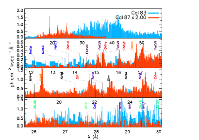
Figure 1: Comparison of high-resolution X-ray spectra of the prototype SSSs Cal 83 (Chandra ObsID 1900) and Cal 87 (XMM-Newton ObsID 0153250101), both located in the LMC. In the bottom panel, blackbody fits are used to illustrate that Cal 83 is an atmosphere spectrum while Cal 87 hosts strong emission lines on top of blackbody-like continuum.

With the advent of the high-resolution X-ray gratings, operated on board the XMM-Newton ($R=0.004$ at 1 keV) and Chandra ($R=0.001$ at 1 keV) missions, it became possible to resolve important details that are needed to better constrain atmosphere models, such as elemental abundances from the depth of absorption lines. From low-resolution spectra, only very rough abundance patterns can be estimated from the depth of absorption edges. The first X-ray grating spectra of SSSs were taken of the prototype SSSs Cal 83 and Cal 87, and a comparison of these spectra is shown in Fig. 1. Even though, both sources are at the same distance, they differ in flux by a factor two (although Cal 87 is slightly brighter at higher energies), but more strikingly, the spectrum of Cal 87 is an emission line spectrum while Cal 83 resembles more an atmosphere spectrum which was successfully modeled with a non-LTE atmosphere model by Lanz et al. (2005). The low-resolution spectrum of Cal 87, shown by Parmar et al. (1997a), is more structured, but the data quality is low enough to consider the structure as Poisson noise. A blackbody fit and an atmosphere model fit still yield good fits to the poor data while the high-resolution spectra now show that both models are wrong. A very similar grating spectrum to that of Cal 87 was found by (Ness et al., 2012) with the recurrent nova U Sco that is an eclipsing system, leading Ness et al. (2013) to conclude that SSS spectra like that of Cal 87 (which is also eclipsing) are strongly affected by obscuration effects, e.g., by an accretion disc in a high-inclination system. In the bottom panel of Fig. 1, blackbody fits illustrate that for Cal 87, there is weak underlying atmospheric continuum emission, possibly originating from the surface, a fraction of which getting to the observer via Thomson Scattering (Ness et al., 2012). Assuming the bolometric luminosity within reasonable limits, the observed effective temperature (Wien tail) requires a radius of the pseudo photosphere to be small enough that it must be fully eclipsed by the companion around phase 0. The fact that we see continuum emission requires the continuum emission to have undergone some scattering processes. The fact that the continuum is not spectrally distorted indicates that the scattering mechanism is independent of photon energy, thus the conclusion by Ness et al. (2012) that we are dealing with Thomson scattering.

3 Analysing high-resolution SSS spectra with atmosphere models

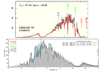
Figure 2: Two independent approaches for fitting atmosphere models to the same data set (Nova V4743 Sgr, day 180 after outburst, Chandra ObsID 3775 (day 180)) by Rauch et al. (2010) (top) and by van Rossum (2012) (bottom).

After Krautter et al. (1996) made a strong case that blackbody fits are not reliable, several approaches were attempted to use atmosphere models. In the most central core of an atmosphere model, there is still a blackbody model (source function), and the Stefan-Boltzmann law also applies to atmosphere models - at least on a qualitative level. While the blackbody model makes the extremely simplifying assumption of thermal equilibrium (TE), the next step foreward is to assume local thermal equilibrium (LTE, e.g., Balman et al. (1998)). More modern codes compute non-LTE (NLTE) atmospheres. One such code developed for white dwarfs is the plane-parallel hydrostatic atmosphere code TMAP (Tübingen NLTE Model-Atmosphere Package). This code has proven particularly useful for compact objects such as isolated white dwarfs, e.g. Werner et al. (2012) or neutron stars, e.g. Rauch et al. (2008). In the limit of highly compact objects, a plane parallel geometry yields similar results as a spherically symmetric geometry which is computationally more expensive. A second important atmosphere code is the PHOENIX code by P. Hauschildt that solves the NLTE radiative transport equations in a co-moving frame, thus allowing expanding ejecta to be modelled. Based on PHOENIX, a wind-type model for SSS spectra has been developed by van Rossum (2012).

The first nova observed as a transient SSS with an X-ray grating was V4743 Sgr (Ness et al., 2003), and five SSS spectra where taken at different times during the evolution of this outburst. This dataset allows detailed conclusions about the evolution of the ejecta during the SSS phase. Two independent analyses with atmosphere models were performed by Rauch et al. (2010) (based on TMAP) and by van Rossum (2012) with examples of their models compared to data shown in Fig. 2. One can see that agreement with the overall shape has been achieved in both cases while there are substantial differences in the details. No statistical goodness criterion like $\chi^{2}$ was given, and from a statistical point of view, both fits are unacceptable. In Fig. 3, I compare the evolution of the parameters effective temperature (middle panel) and $N_{\rm H}$ (bottom) derived from the two approaches and a simple blackbody fit. The effective temperature systematically differs by $\sim 25$%. van Rossum (2012) has assumed a constant value of $5.5\times 10^{5}$ K while Rauch et al. (2010) have iterated this parameter, detecting small variations above $7\times 10^{5}$ K. A blackbody fit yields the lowest effective temperature values. The trends in temperature evolution differ only slightly. The TMAP model shows a small increase in temperature until day 300 and a continuous decline thereafter. Meanwhile, the wind-type model can explain the changes that the TMAP model attributes to temperature changes to changes in other parameters and thus concludes the observations to be consistent with constant effective temperature until day 370 and only then a decrease. The blackbody fits yield the largest changes in best-fit effective temperature which is likely a result of ignoring any absorption that may be variable.

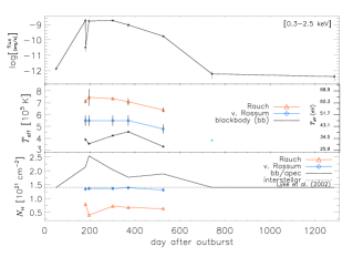
Figure 3: Comparison of atmosphere model parameters of the two models by Rauch et al. (2010) and by van Rossum (2012). The observed (absorbed) fluxes shown in the top have been derived by integration of the fluxes in each wavelength bin.

Shortly after the outburst, the amount of interstellar absorption by neutral hydrogen was determined by Lyke et al. (2002) with $1.4\times 10^{21}$ cm^-2, based on a method by Gehrz et al. (1974) that was also employed by Gehrz et al. (2015) for the nova V339 Del, also giving some more details. Interestingly, exactly the same value was found by van Rossum (2012) who argues that $N_{\rm H}$ requires special attention prior to any adjustment of atmosphere model parameters. Small variations in $N_{\rm H}$ imply large differences in assumed fluxes at long (EUV) wavelengths at which hardly any flux is observed. Therefore, poor values of $N_{\rm H}$ will hardly be penalised by $\chi^{2}$ fitting even though strong assumptions are made about the invisible part of the spectrum. After careful pre-adjustment of $N_{\rm H}$, the values determined by van Rossum (2012) are all spot on with those derived by Lyke et al. (2002). I emphasise here that Lyke et al. (2002) was not quoted by van Rossum (2012), indicating that van Rossum (2012) was not biased by the literature value. Meanwhile, the $N_{\rm H}$ values derived by Rauch et al. (2010), determined by fitting $N_{\rm H}$ simultaneously with other atmosphere parameters, are all well below the value derived by Lyke et al. (2002) (which was also not quoted). This can either mean that Lyke et al. (2002) overestimated $N_{\rm H}$, that the value of $N_{\rm H}$ was lower during the SSS phase, or that Rauch et al. (2010) underestimate $N_{\rm H}$. Meanwhile, the values of $N_{\rm H}$ from the blackbody fits are all much higher which can either mean that local absorption was higher during the SSS phase or that the blackbody fit overestimates $N_{\rm H}$. As all of the spectral fits have unacceptable goodness of fit, it is also possible that all of the derived parameter values are incorrect.

The reason why the effective temperature can be underestimated while $N_{\rm H}$ is overestimated can be explained as follows:

• If the ionisation energy of an abundant element such as nitrogen coincides with the Wien tail, a significant amount of high-energy emission is missing.

• A model not accounting for ionisation absorption edges will see the Wien tail at longer wavelengths, thus underestimating the effective temperature.

• A model with underestimated effective temperature will overpredict the emission at soft energies, and rigorous parameter fitting will increase $N_{\rm H}$ in order to get rid of the excess soft emission.

Inversely, if the effects of absorption edges in the Wien tail are overestimated, then effective temperatures are overestimated and $N_{\rm H}$ underestimated. The large differences between the two atmosphere models in $N_{\rm H}$ can thus be a consequence of the difference in effective temperature, and it is of high importance that the absorbing behaviour of the outer ejecta is well understood in order to derive reliable principle parameters.

4 The annoying little details

In the following subsections, a few effects are described that are seen in the observed spectra that complicate any quantitative analysis based on global models.

4.1 Blue shifts

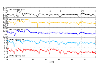
Figure 4: Evolution of absorption lines in the two novae SMC 2016 (top three panels, Chandra ObsIDs 19011/19012 (days 38.9 and 86.2) and XMM-Newton ObsID 0794180201 (day 73.8)) and V4743 Sgr (bottom two panels, Chandra ObsIDs 3775 (day 180) and 3776 (day 302)). Dotted lines mark a N vi resonance line (28.8 Å), an unidentified line at $\sim 30.5$ Å, an interstellar N i 1s-2p line at 31.3 Å, another unidentified line at $\sim 32.1$ Å, and a C vi resonance line at 33.7 Å. The N vi and C vi lines are blue shifted by the same amount during the evolution indicating continuous expanding absorbing material (see § 4.1). The unidentified line at 32.1 Å undergoes strange changes. In SMC 2016, it was only present in the first observation while in V4743 Sgr, it has changed from 32 Å to 32.1 Å (see § 4.2).

Already the first SSS spectrum of a nova, V4743 Sgr, displayed absorption lines that are blue-shifted in excess of 2000 km s^-1 (Ness et al., 2003). Ness (2010) showed that line blue shifts are observed in many nova SSS spectra. In Fig. 4, some example spectra are shown where the blue shifts can be seen in two resonance lines of N vi and C vi. We have determined the blue shifts with Gauss fits to the respective absorption lines and show the results in Fig. 5. In SMC 2016, the expansion velocity has increased from day 38.9 to day 86.2 (47 days) by $\sim 20$% in both lines while in V4743 Sgr, it has only increased, from day 180 to day 203 (122 days), by $\sim 3$%. The increase of observed blue shifts may indicate that during the evolution of the SSS phase, the photospheric radius has continued to shrink into a regime with higher velocity, and the outflow is thus not constant with radius.

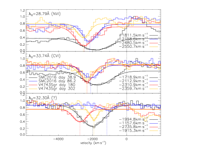
Figure 5: Comparison of line profiles of four spectra shown in Fig. 4 (see text).

The observed blue-shifted lines may either be formed in an optically thin wind or in the ejecta. In SMC 2016, one can see evidence for P Cyg profiles in the first observation, whereas the emission component is not present in the later two observations. A similar behaviour was seen in RS Oph (Ness et al., 2007). This may indicate that the mass loss rate can decrease during the SSS phase.

Regardless of whether the absorption lines are formed in an optically thin wind or in the ejecta, both atmosphere model approaches compute the absorption lines as part of the same system. The model by Rauch et al. (2010) is a hydrostatic model that cannot reproduce blue shifts self-consistently, and in order to fit the blue shifts in the observed spectra, a negative red-shift parameter was added. All the dynamics are thus not included, and it is unknown what effect (apart from blue-shifted absorption lines) the expansion can have on the observable spectrum. It is also not confirmed whether the photosphere is already on the surface of the white dwarf or somewhere within the outflow.
The wind-type model by van Rossum (2012) assumes a hydrostatic core with an optically thin wind on top of that and models line blue shifts selfconsistently. The absorption behaviour of the wind can lead to significantly different model spectra compared to pure hydrostatic models, and adjustment to observed spectra can thus lead to much different parameters.
It may be instructive to compare the Rauch et al. (2010) model with the hydrostatic core of the van Rossum (2012) which should lead to consistent results if the different implementations and side assumptions are correct.

4.2 Unidentified lines

The example spectra in Fig. 4 also show two unidentified lines at $\sim 30.5$ Å and $\sim 32.1$ Å in both novae. In SMC 2016, both lines were only present on day 38.9 while in V4743 Sgr, they are seen in both example spectra, albeit with different profiles. Strangely, one line shifted from 32 Å on day 180 to 32.1 Å on day 302. A line shift of 0.1 Å at 32 Å corresponds to almost 1000 km s^-1. Only two spectra are shown as examples, but I looked at all five observation of V4743 Sgr (Chandra ObsIDs 3775 (day 180), 3776 (day 302), 4435 (day 371), and 5292 (day 526) and XMM-Newton ObsID 0127720501 (day 196)) and found that this change already took place between day 180 and day 196 (see bottom panel of Fig. 6) - thus within only two weeks! - and remained at 32.1 Å after day 196. We know nothing about this line, it is obviously not interstellar and thus unlikely to arise from a neutral atom like the N i line at 31.3 Å. If it arises in the same blue-shifted system as the high-ionisation lines of N vi and C vi, the wavelength change in V4743 Sgr suggests a rest wavelength of around 32.3 Å. Various databases give inconsistent results, e.g., there are several lines in NIST around 32.3 Å, e.g., Mg xi, S xiii while Atomdb
(http://www.atomdb.org/Webguide/webguide.php)
lists K xi lines that go to the ground. Such identifications need to be carefully checked for consistency, e.g., with other lines in the same iso-electronic sequence which is beyond of this work. There are numerous other observed absorption lines without clear identifications in other novae, see table 5 in Ness et al. (2011). An approach to identify them would be to assemble a data base with observed wavelengths of unknown lines and the environments in which they are formed such as effective temperature, blue shifts of known absorption lines etc. The identification is important to improve the atomic data underlying the atmosphere models.

4.3 Complex line profiles

In a hydrostatic atmosphere, one expects narrow absorption lines, but we see not only blue-shifted but also broadened absorption lines. This is illustrated in Fig. 6 where the two photospheric lines from Fig. 5 are shown in comparison to the N vii line at 24.74 Å. One can see that the profiles differ dramatically with the N vii line yielding a line width of several thousand km s^-1 while the N vi and C vi lines are much narrower. The line profile of the N vii line is also complex with at least two sub-components that have similar widths as the N vi and C vi lines. One of these components, at $\sim-4000$ km s^-1, has converted from an absorption line on day 180 to an emission line on day 196 but then back to an absorption line day 302; possibly also the lower-blueshift line at $\sim-2500$ km s^-1.

The complexity of the N vii line profile indicates that we are observing several velocity components simultaneously. This observation adds to numerous observational evidence for non-homogeneous or asymmetric outflows from novae such as high-amplitude variations during the early SSS phase (Osborne et al., 2011). Therefore, even the model by van Rossum (2012) is oversimplified.

Figure 6: Comparison of line profiles of three spectra of nova V4743 Sgr at different times of the SSS evolution (see labels). The top three panels compare the profiles of the three photospheric lines of N vi, C vi, and N vii while the bottom panel shows the unidentified line assuming a rest wavelength of 32.3 Å. Best-fit blue shifts are given in the respective bottom right legends.

5 Conclusions

The standard interpretation approach in X-ray astronomy for spectra is to fit spectral models to the observations. When the spectral resolution is low enough that no details are resolved, this approach yields acceptable fits with already quite simple models. If resulting parameters are unrealistic, more complex models need to be tested, but it brings about the problem that such models are overdetermined when fitted to low-resolution spectra with only a few hundred spectral bins.

With the advent of high-resolution X-ray spectra, a paradigm shift would be necessary, but this has not been realised yet.

Highly complex atmosphere models provide of course more physics than blackbody fits, however, they only give acceptable fits when fitted to low-resolution spectra. No atmosphere model has so far been found that reproduces an SSS grating spectra in all the details. A quantitative assessment of the goodness of fit appears hopeless at this time, and the best that has been achieved was qualitative agreement with data.

So, are the atmosphere models useless? And what can actually be learned from the high-quality SSS grating spectra?

I propose to use the atmosphere models for the interpretation of the data rather than trying to determine physical, quantitative parameters. It is of course important to get a handle on the effective temperature - but what does it help if we can never be sure whether we have actually determed the correct value? Rather than believing we have found the correct values, we should consider any values found as an assumption because they depend on the assumptions behind the models.

An example use case for the atmosphere models is the identification of the absorption lines which is tricky because each identification needs to be consistent with the rest of the spectrum. It is not enough to consult an atomic database for the strongest line at a given wavelength. Any candidate identification needs to be checked for consistency, e.g., which other lines should then be seen or not seen. Doing this manually is at best tedious because one would have to go through the entire multiplet, finding the strongest lines and compare which ones are seen at the expected wavelengths and with the expected strengths. It would not be possible to account for complex processes such as line emission and self absorption (thus radiation transport), and an atmosphere model would be the only possibility to determine line identifications under complex conditions in a self-consistent way.

When looking beyond X-ray astronomy, one will encounter numerous methods of interpretations, e.g., of optical spectra, not using any models at all. Optical spectra are traditionally of too high quality that it was hopeless from the start to find any model that could give quantitative parameter values. Yet, a lot has been learned from optical spectra by classifying spectra by presence or absence of certain lines, creating classifications based on anomalously strong or weak types of lines etc. The limited spectral resolution of X-ray observations has not allowed such approaches so far, but after almost 20 years of having high-resolution grating spectra, it is time to explore more such methods. An example is the classification of SSS spectra dominated by emission or absorption lines by Ness et al. (2013).

A way forward would be to study the diverse absorption line profiles, identify the corresponding transitions and classify lines behaving similarly in order to determine the dynamics in the different regions of the outflow. The formation characteristics of each line give physical information such as temperature, so one can qualitatively localise the emission region, assuming a radial temperature profile.

Future high-energy observatories such as XRISM or Athena will provide more high-resolution spectra, and I predict the days of model fitting to low-resolution spectra to be counted.

References

- Balman et al. (1998) Balman, S., Krautter, J., Ögelman, H., 1998. The X-Ray Spectral Evolution of Classical Nova V1974 Cygni 1992: A Reanalysis of the ROSAT Data. ApJ 499, 395–406.
- Gehrz et al. (2015) Gehrz, R.D., Evans, A., Helton, L.A., Shenoy, D.P., Banerjee, D.P.K., Woodward, C.E., Vacca, W.D., Dykhoff, D.A., Ashok, N.M., Cass, A.C., 2015. The Early Infrared Temporal Development of Nova Delphini 2013 (V339 DEL) Observed with the Stratospheric Observatory for Infrared Astronomy (SOFIA) and from the Ground. ApJ 812, 132–143. doi:10.1088/0004-637X/812/2/132.
- Gehrz et al. (1974) Gehrz, R.D., Hackwell, J.A., Jones, T.W., 1974. Infrared observations of Be stars from 2.3 to 19.5 microns. ApJ 191, 675–684. doi:10.1086/153008.
- Henze et al. (2014) Henze, M., Ness, J.U., Darnley, M.J., Bode, M.F., Williams, S.C., Shafter, A.W., Kato, M., Hachisu, I., 2014. A remarkable recurrent nova in M 31: The X-ray observations. A&A 563, L8–L12. doi:10.1051/0004-6361/201423410, arXiv:1401.2904.
- Kahabka and van den Heuvel (1997) Kahabka, P., van den Heuvel, E.P.J., 1997. Luminous Supersoft X-Ray Sources. ARA&A 35, 69–100.
- Krautter et al. (1996) Krautter, J., Ögelman, H., Starrfield, S., Wichmann, R., Pfeffermann, E., 1996. ROSAT X-Ray Observations of Nova V1974 Cygni: The Rise and Fall of the Brightest Supersoft X-Ray Source. ApJ 456, 788–797.
- Lanz et al. (2005) Lanz, T., Telis, G.A., Audard, M., Paerels, F., Rasmussen, A.P., Hubeny, I., 2005. Non-LTE Model Atmosphere Analysis of the Large Magellanic Cloud Supersoft X-Ray Source CAL 83. ApJ 619, 517–526.
- Lyke et al. (2002) Lyke, J.E., Kelley, M.S., Gehrz, R.D., Woodward, C.E., 2002. Free-Free Turnover in Nova V4743 Sgr 2002 #3. Bulletin of the American Astronomical Society 34, 1161.
- Ness (2010) Ness, J., 2010. Observational evidence for expansion in the SSS spectra of novae. Astronomische Nachrichten 331, 179–182. doi:10.1002/asna.200911322, arXiv:0908.4549.
- Ness et al. (2012) Ness, J., Schaefer, B.E., Dobrotka, A., Sadowski, A., Drake, J.J., Barnard, R., Talavera, A., Gonzalez-Riestra, R., Page, K.L., Hernanz, M., Sala, G., Starrfield, S., 2012. From X-Ray Dips to Eclipse: Witnessing Disk Reformation in the Recurrent Nova U Sco. ApJ 745, 43–58. doi:10.1088/0004-637X/745/1/43, arXiv:1105.2717.
- Ness et al. (2007) Ness, J., Starrfield, S., Beardmore, A., Bode, M.F., Drake, J.J., Evans, A., Gehrz, R., Goad, M., Gonzalez-Riestra, R., Hauschildt, P., Krautter, J., O’Brien, T.J., Osborne, J.P., Page, K.L., Schönrich, R., Woodward, C., 2007. The SSS phase of RS Ophiuchi observed with Chandra and XMM I. Data and preliminary Models. ApJ 665, 1334–1348. arXiv:astro-ph/0705.1206.
- Ness et al. (2003) Ness, J., Starrfield, S., Burwitz, V., Wichmann, R., Hauschildt, P., Drake, J.J., Wagner, R.M., Bond, H.E., Krautter, J., Orio, M., Hernanz, M., Gehrz, R.D., Woodward, C.E., Butt, Y., Mukai, K., Balman, S., Truran, J.W., 2003. A Chandra Low Energy Transmission Grating Spectrometer Observation of V4743 Sagittarii: A Supersoft X-Ray Source and a Violently Variable Light Curve. ApJL 594, L127–L130.
- Ness et al. (2011) Ness, J.U., Osborne, J.P., Dobrotka, A., Page, K.L., Drake, J.J., Pinto, C., Detmers, R.G., Schwarz, G., Bode, M.F., Beardmore, A.P., Starrfield, S., Hernanz, M., Sala, G., Krautter, J., Woodward, C.E., 2011. XMM-Newton X-ray and Ultraviolet Observations of the Fast Nova V2491 Cyg during the Supersoft Source Phase. ApJ 733, 70–85. doi:10.1088/0004-637X/733/1/70, arXiv:1103.4543.
- Ness et al. (2013) Ness, J.U., Osborne, J.P., Henze, M., Dobrotka, A., Drake, J.J., Ribeiro, V.A.R.M., Starrfield, S., Kuulkers, E., Behar, E., Hernanz, M., Schwarz, G., Page, K.L., Beardmore, A.P., Bode, M.F., 2013. Obscuration effects in super-soft-source X-ray spectra. A&A 559, 1–15. doi:10.1051/0004-6361/201322415, arXiv:1309.2604.
- Osborne et al. (2011) Osborne, J.P., Page, K.L., Beardmore, A.P., Bode, M.F., Goad, M.R., O’Brien, T.J., Starrfield, S., Rauch, T., Ness, J., Krautter, J., Schwarz, G., Burrows, D.N., Gehrels, N., Drake, J.J., Evans, A., Eyres, S.P.S., 2011. The Supersoft X-ray Phase of Nova RS Ophiuchi 2006. ApJ 727, 124–123. doi:10.1088/0004-637X/727/2/124, arXiv:1011.5327.
- Parmar et al. (1997a) Parmar, A.N., Kahabka, P., Hartmann, H.W., Heise, J., Martin, D.D.E., Bavdaz, M., Mineo, T., 1997a. A BeppoSAX observation of the super-soft source CAL87. A&A 323, L33–L36. arXiv:arXiv:astro-ph/9706008.
- Parmar et al. (1998) Parmar, A.N., Kahabka, P., Hartmann, H.W., Heise, J., Taylor, B.G., 1998. A BeppoSAX LECS observation of the super-soft X-ray source CAL 83. A&A 332, 199–203. arXiv:arXiv:astro-ph/9712040.
- Parmar et al. (1997b) Parmar, A.N., Martin, D.D.E., Bavdaz, M., Favata, F., Kuulkers, E., Vacanti, G., Lammers, U., Peacock, A., Taylor, B.G., 1997b. The low-energy concentrator spectrometer on-board the BeppoSAX X-ray astronomy satellite. AAPS 122, 309–326. doi:10.1051/aas:1997137.
- Rauch et al. (2010) Rauch, T., Orio, M., Gonzales-Riestra, R., Nelson, T., Still, M., Werner, K., Wilms, J., 2010. Non-local Thermal Equilibrium Model Atmospheres for the Hottest White Dwarfs: Spectral Analysis of the Compact Component in Nova V4743 Sgr. ApJ 717, 363–371. doi:10.1088/0004-637X/717/1/363, arXiv:1006.2918.
- Rauch et al. (2008) Rauch, T., Suleimanov, V., Werner, K., 2008. Absorption features in the spectra of X-ray bursting neutron stars. A&A 490, 1127–1134. doi:10.1051/0004-6361:200810129, arXiv:0809.2170.
- Schwarz et al. (2011) Schwarz, G.J., Ness, J., Osborne, J.P., Page, K.L., Evans, P.A., Beardmore, A.P., Walter, F.M., Helton, L.A., Woodward, C.E., Bode, M., Starrfield, S., Drake, J.J., 2011. Swift X-Ray Observations of Classical Novae. II. The Super Soft Source Sample. ApJS 197, 31–56. doi:10.1088/0067-0049/197/2/31, arXiv:1110.6224.
- van den Heuvel et al. (1992) van den Heuvel, E.P.J., Bhattacharya, D., Nomoto, K., Rappaport, S.A., 1992. Accreting white dwarf models for CAL 83, CAL 87 and other ultrasoft X-ray sources in the LMC. A&A 262, 97–105.
- van Rossum (2012) van Rossum, D.R., 2012. A Public Set of Synthetic Spectra from Expanding Atmospheres for X-Ray Novae. I. Solar Abundances. ApJ 756, 43–53. doi:10.1088/0004-637X/756/1/43, arXiv:1205.4267.
- Werner et al. (2012) Werner, K., Rauch, T., Ringat, E., Kruk, J.W., 2012. First Detection of Krypton and Xenon in a White Dwarf. ApJL 753, L7–L11. doi:10.1088/2041-8205/753/1/L7.