Integrable systems in planar robotics

Abstract.

The main purpose of this paper is to investigate commuting flows and integrable systems on the configuration spaces of planar linkages. Our study leads to the definition of a natural volume form on each configuration space of planar linkages, the notion of cross products of integrable systems, and also the notion of multi-Nambu integrable systems. The first integrals of our systems are functions of Bott-Morse type, which may be used to study the topology of configuration spaces.

Dedicated to Anatoly T. Fomenko on the occasion of his 75th birthday

1. Introduction

This paper is a preliminary investigation of natural commuting flows and integrable systems on the configuration spaces of linkages in geometry, machinery and robotics, especially planar linkages. Our motivation is manifold:

$\bullet$ Firstly, linkages appear everywhere in mechanical systems (see, e.g., [18, 26]). Moreover, commuting flows may be viewed as “independent components” in a mechanical system and play an important role in robotics and motion control: the commutativity makes it easier to compute and control the motions. In fact, one may observe many commuting flows in practice. For example, the excavator in Figure 1 (left), borrowed from Servatius et al. [23] with permission, has two sliding mechanisms, which commute with each other. This excavator may be represented by a planar linkage in Figure 1 (right), where each sliding mechanism is replaced by two connecting edges. The configuration space of this linkage admits an integrable system having two commuting vector fields. If one allows some of the lengths of the edges to be variable, then the configuration space has higher dimension, and those adjustable lengths are first integrals of the integrable system in question.

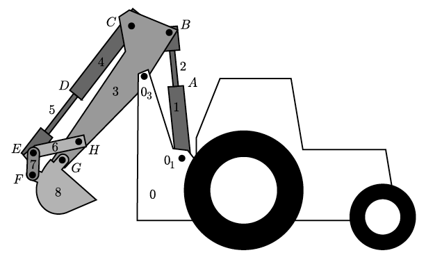
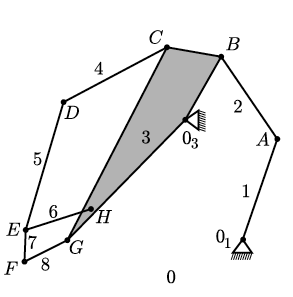
Figure 1. The excavator and its planar linkage representation, after [23].

$\bullet$ Secondly, for 3-dimensional (3D) polygonal linkages, there are now famous bending flows (around diagonals) found by Kapovich and Millson [15], which are a special class of integrable Hamiltonian systems, and the singularities of these systems have been described in a recent paper by Bouloc [3]. We want to see to what extent these results can be generalized to other situations, especially planar linkages, and also 3D linkages which are more general than just polygons. It turns out that, for 2-dimensional (2D) polygons, we have a simple construction which may be viewed as an analogue of Kapovich-Millson systems: given a 2D $n$-gonal linkage ($n\geq 4$), just choose arbitrary $[(n-3)/2]$ ($[\cdot]$ denotes the integer part of a real number) non-crossing diagonals which decomposes it into $[n/2]-1$ quadrangles and at most one triangle (one if $n$ is odd and zero if $n$ is even). Then we get a non-Hamiltonian integrable system on the configuration space of type $([n/2]-1,[(n-3)/2])$, i.e., with $[n/2]-1$ commuting vector fields and $[(n-3)/2]$ common first integrals; ($[(n-3)/2]+[n/2]-1=n-3$ is the dimension of the configuration space). Each diagonal gives one first integral (its length, or rather its length squared to be smooth), each quadrangle has one degree of freedom and gives rise to one vector field, and they all commute with each other (see the rest of this paper for details). For example, when $n=7$, the configuration space of a generic planar heptagonal linkage is a 4-dimensional manifold, on which we have integrable systems of type (2,2), i.e., with two commuting vector fields and two common first integrals, by this construction.

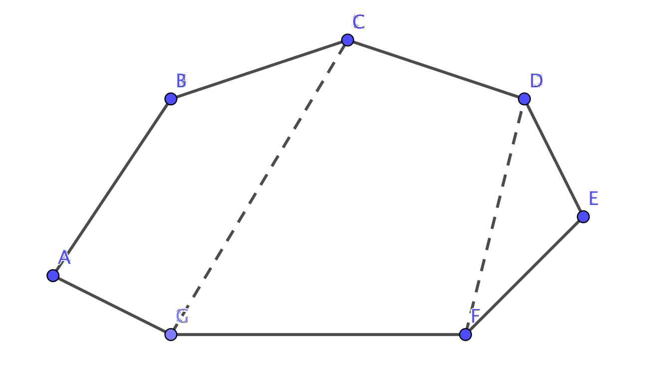
Figure 2. An integrable system on a the 4-dimensional configuration space of a 7-gon linkage: the two “4-bar mechanisms” $ABCG$ and $CGFD$ provide two commuting vector fields and the square lengths $|CG|^{2}$ and $|DF|^{2}$ are their smooth common first integrals.

Recall that the configuration space of 3D linkages admits a natural symplectic structure [19, 15, 10]. However, for 2D linkages, a priori, we have neither a natural symplectic structure, nor Hamiltonian systems; however, we have Nambu structures and so our vector fields can be constructed in the spirit of Nambu mechanics [22]. Recall that a Nambu structure of order $q$ on a manifold is a $q$-vector field which spans a (singular) integrable $q$-dimensional distribution and which may be viewed as a leaf-wise contravariant volume element on the corresponding singular $q$-dimensional foliation; see, e.g., [4, 20]. Contravariant volume elements are particular cases of Nambu structures and they were used by Nambu in [22] as a way to generalize Hamiltonian mechanics, whence the name.

$\bullet$ Our third motivation is given by the universality theorem of Kapovich and Millson [16], which was announced many years before by Thurston [24] but without a full proof. This theorem states that, given any closed (compact without boundary) smooth manifold, there is a planar linkage whose configuration space is diffeomorphic to a disjoint union of a finite number of copies of that manifold. Thus, by studying natural integrable systems on configuration spaces of planar linkages, we can obtain interesting integrable non-Hamiltonian systems on any closed manifold. The theory of integrable non-Hamiltonian systems (in the sense of Bogoyavlensky [2]) is relatively new compared to integrable Hamiltonian systems, especially when it comes to their topological and geometric properties (see [27] and references therein), so this huge class of integrable non-Hamiltonian systems coming from planar linkages will be very useful for the development of the theory. We summarize below the main results of the paper.

The first result of this paper, presented in Section 2, is that every configuration space of planar linkages admits a natural volume form. This volume form, together with a choice of diagonals in the linkage, gives rise to Nambu structures on the configuration space.

In Section 3 we give a simple general method for constructing integrable systems on configuration spaces of planar linkages, by decomposing such spaces into cross products of smaller configuration spaces, and lifting integrable systems from these smaller spaces. In particular, we introduce the notion of cross products of integrable systems in this section and, as a special case of this cross product construction, we find, what we call, multi-Nambu integrable systems.

In Section 4, the last section of this paper, we list some open questions and final remarks. In particular, we mention that our first integrals are Bott-Morse functions on many configuration spaces, which are helpful in topology. For example, in the case of hexagons, by using these Bott-Morse functions, one immediately gets the fact that the corresponding configuration spaces belong to a special class of very well-studied 3-manifolds named graph-manifolds by Waldhausen [25]; this fact also fits well with Fomenko’s topological theory of integrable systems on 3-manifolds [7].

2. Configuration spaces of planar linkages

2.1. Definition of the orbit and configuration spaces

In this paper, a planar linkage $\mathcal{L}$ consists of:

• A finite graph $\mathcal{G}=(\mathcal{V},\mathcal{E})$, where $\mathcal{V}$ denotes the set of vertices and $\mathcal{E}$ denotes the set of edges of $\mathcal{G}$. For any two vertices $A,B\in\mathcal{V}$ there is at most one edge connecting them, denoted $AB$ or $BA$. An edge is also called a bar in $\mathcal{L}$.

• Each edge has an associated positive length, i.e., there is a length function

  $$\ell:\mathcal{E}\to\mathbb{R}_{+}:=\,]0,\infty[$$

  which specifies the length $\ell(AB)$ of each edge $AB\in\mathcal{E}$.

• A subset $\mathcal{B}\subset\mathcal{V}$ of vertices, which may be empty, called the set of fixed vertices or based points, which comes together with a fixing map

  $$\beta:\mathcal{B}\to\mathbb{R}^{2}$$

  that attaches $\mathcal{L}$ to the Euclidean plane $\mathbb{R}^{2}$. The vertices in $\mathcal{V}\setminus\mathcal{B}$ are called movable.

The pair $(\mathcal{G},\mathcal{B})$, where the lengths and the fixing are not specified, is called the linkage type of $\mathcal{L}$.

A realization of a planar linkage $\mathcal{L}=(\mathcal{V},\mathcal{E},\ell,\mathcal{B},\beta)$ is a map

$$\mathbf{r}:\mathcal{V}\to\mathbb{R}^{2}$$

which respects the based points and the bar lengths. In other words,

$$|\mathbf{r}(A)\mathbf{r}(B)|=\ell(AB),$$

for any $A,B\in\mathcal{V}$, and the restriction of $\mathbf{r}$ to the set $\mathcal{B}$ of base vertices coincides with $\beta$. Of course, the length condition means that $\mathbf{r}$ can be extended to a map from the whole graph $\mathcal{G}$ to $\mathbb{R}^{2}$, that maps each edge of $\mathcal{G}$ to a straight line segment of the same length. In a planar realization of a linkage, the bars can cross each other, i.e., we do not require the map from the graph to $\mathbb{R}^{2}$ to be injective. The crossing of bars may be realized in practice by laying them on parallel planes.

The space of all realizations of a planar linkage $\mathcal{L}$ is denoted by $\mathcal{O}_{\mathcal{L}}$; it is also called the orbit space of $\mathcal{L}$. Two different realizations $\mathbf{r}_{1}$, $\mathbf{r}_{2}$ of $\mathcal{L}$ are said to be isometric if there is an orientation and length preserving map $\phi:\mathbb{R}^{2}\rightarrow\mathbb{R}^{2}$ (i.e., $\phi\in SE(2)$, the Euclidean group) such that $\phi\circ\mathbf{r}_{1}=\mathbf{r}_{2}$. The set of all realizations of $\mathcal{L}$ modulo isometries is called the configuration space and is denoted by $M_{\mathcal{L}}$.

If $\mathcal{B}=\emptyset$ is empty then the realizations of $\mathcal{L}$ can move freely in $\mathbb{R}^{2}$; in this case $SE(2)$ acts on $\mathcal{O}_{\mathcal{L}}$, the action is free if $\mathcal{L}$ has at least one bar, and we have

$$M_{\mathcal{L}}=\mathcal{O}_{\mathcal{L}}/SE(2).$$

If $\mathcal{B}$ consists of exactly one base point $B$, then the configurations cannot be translated freely in $\mathbb{R}^{2}$ but can turn around $B$; in this case we have

$$M_{\mathcal{L}}=\mathcal{O}_{\mathcal{L}}/SO(2).$$

If, however, $\mathcal{B}$ consists of at least two distinct base vertices, then two realizations of $\mathcal{L}$ are isometric if and only if they coincide; in this case we have

$$M_{\mathcal{L}}=\mathcal{O}_{\mathcal{L}}.$$

Let $G_{\mathcal{L}}$ be the group $\{e\}$, $SO(2)$, or $SE(2)$, depending on whether $\mathcal{B}$ has at least two, one, or zero fixed vertices. With this notation, in view of the considerations above, we have $M_{\mathcal{L}}=\mathcal{O}_{\mathcal{L}}/G_{\mathcal{L}}$.

Note that when studying the configuration space of a linkage, we can choose between the version with at least 2 base points and the version without any base point. Indeed, if $\mathcal{L}=(\mathcal{V},\mathcal{E},\ell,\mathcal{B},\beta)$, where $\mathcal{B}$ has at least 2 points, then we can add all edges $BC$ with vertices $B,C\in\mathcal{B}$, together with their lengths $\ell(BC)=|\beta(B)\beta(C)|$, then forget these base vertices, and we get a linkage with empty base. This new linkage, now without any base vertices, has the same configuration space as the old linkage. Conversely, if $\mathcal{L}$ does not have any base points, then we can choose an arbitrary bar in $\mathcal{L}$ and fix it to $\mathbb{R}^{2}$, so that its vertices become base points, without changing the configuration space of $\mathcal{L}$.

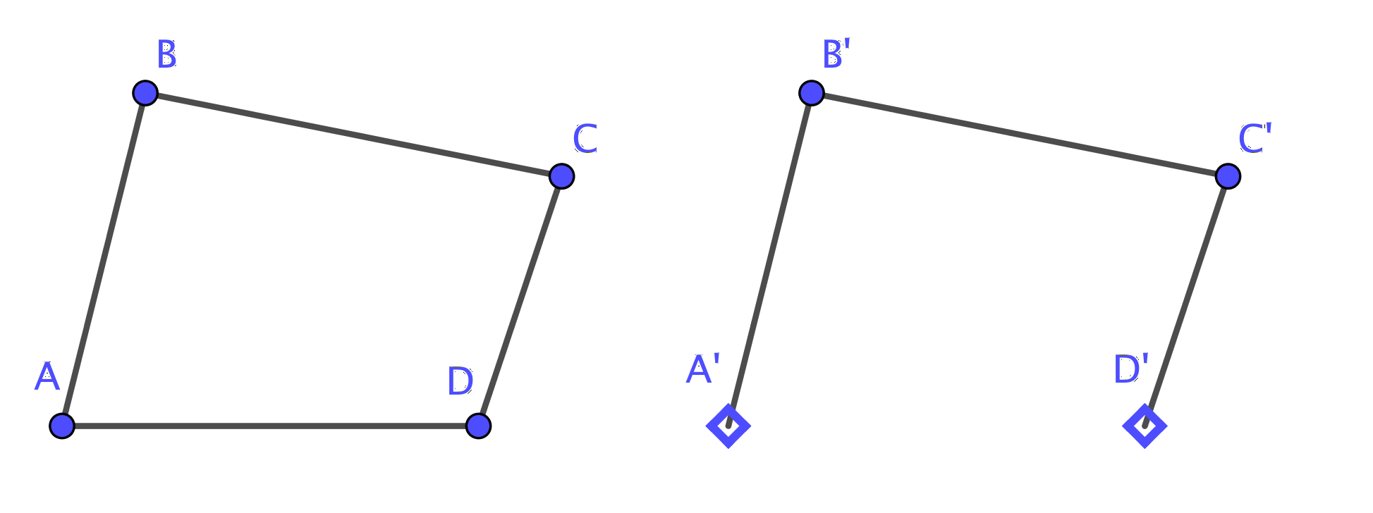
Figure 3. Two versions of a quadrangle (with and without base points), also called a 4-bar mechanism, with the same configuration space.

For example, consider a quadrangle linkage $\mathcal{L}$ (also called a 4-bar mechanism) consisting of four vertices $A,B,C,D$ and four edges with four fixed lengths $\ell_{1}=|AB|$, $\ell_{2}=|BC|$, $\ell_{3}=|CD|,\ell_{4}=|DA|$, and no base point. Consider the same quadrangle, but now with two base points $A$ and $D$, and only three free edges $AB$, $BC$, $CD$ (the edge $DA$ can be removed because $A$ and $D$ are already fixed). We get a new linkage $\mathcal{L}_{2}$, whose configuration space is exactly the same as the configuration space of $\mathcal{L}_{1}$ (see Figure 3).

Remark 2.1.

When talking about a linkage $\mathcal{L}$, one often assumes that it is connected (i.e., the corresponding graph is connected). However, for our study, it is convenient to allow linkages which are disconnected. It is clear that if $\mathcal{L}$ is a disjoint union of two linkages $\mathcal{L}_{1}$ and $\mathcal{L}_{2}$, then its base is also the disjoint union of $\mathcal{B}_{1}$ and $\mathcal{B}_{2}$ and its orbit space is simply the direct product of the two corresponding orbit spaces:

$$\mathcal{O}_{\mathcal{L}_{1}\sqcup\mathcal{L}_{2}}=\mathcal{O}_{\mathcal{L}_{1}}\times\mathcal{O}_{\mathcal{L}_{2}}.$$

The formula for the configuration space of ${\mathcal{L}_{1}\sqcup\mathcal{L}_{2}}$ is more complicated. Namely, we have six cases:

(i) If both $\mathcal{B}_{1}$ and $\mathcal{B}_{2}$ have at least two vertices, then $\mathcal{O}_{\mathcal{L}}=M_{\mathcal{L}}=\mathcal{O}_{\mathcal{L}_{1}}\times\mathcal{O}_{\mathcal{L}_{2}}=M_{\mathcal{L}_{1}}\times M_{\mathcal{L}_{2}}$.

(ii) If $\mathcal{B}_{1}$ has at least two vertices and $\mathcal{B}_{2}$ consists of exactly one vertex, then $\mathcal{O}_{\mathcal{L}}=M_{\mathcal{L}}=\mathcal{O}_{\mathcal{L}_{1}}\times\mathcal{O}_{\mathcal{L}_{2}}$ but $M_{\mathcal{L}_{1}}\times M_{\mathcal{L}_{2}}=M_{\mathcal{L}}/SO(2)$, the $SO(2)$-action being on the second factor.

(iii) If $\mathcal{B}_{1}$ has at least two vertices and $\mathcal{B}_{2}=\emptyset$, then $\mathcal{O}_{\mathcal{L}}=M_{\mathcal{L}}=\mathcal{O}_{\mathcal{L}_{1}}\times\mathcal{O}_{\mathcal{L}_{2}}$ but $M_{\mathcal{L}_{1}}\times M_{\mathcal{L}_{2}}=M_{\mathcal{L}}/SE(2)$, the $SE(2)$-action being on the second factor.

(iv) If both $\mathcal{B}_{1}$ and $\mathcal{B}_{2}$ have each exactly one vertex, then $\mathcal{O}_{\mathcal{L}}=M_{\mathcal{L}}=\mathcal{O}_{\mathcal{L}_{1}}\times\mathcal{O}_{\mathcal{L}_{2}}$ but $M_{\mathcal{L}_{1}}\times M_{\mathcal{L}_{2}}=M_{\mathcal{L}}/(SO(2)\times SO(2))$, each $SO(2)$ acting separately on its corresponding factor.

(v) If $\mathcal{B}_{1}$ consists of one vertex and $\mathcal{B}_{2}=\emptyset$, then $M_{\mathcal{L}}=\mathcal{O}_{\mathcal{L}}/SE(2)=\mathcal{O}_{\mathcal{L}_{1}}\times_{SO(2)}\mathcal{O}_{\mathcal{L}_{2}}$, so we get fibrations $M_{\mathcal{L}}\rightarrow\mathcal{O}_{\mathcal{L}_{1}}$, $M_{\mathcal{L}}\rightarrow\mathcal{O}_{\mathcal{L}_{2}}$ whose fibers are $\mathcal{O}_{\mathcal{L}_{2}}$ and $\mathcal{O}_{\mathcal{L}_{1}}$, respectively. Thus we get an $SE(2)$-principal fiber bundle $M_{\mathcal{L}}\rightarrow M_{\mathcal{L}_{1}}\times M_{\mathcal{L}_{2}}$. The $SE(2)$-action is induced from the following $SE(2)$-action on the linkage: fix a second vertex on $\mathcal{L}_{1}$ and let $SE(2)$ act on $\mathcal{L}_{2}$. The resulting action on $M_{\mathcal{L}}$ is free and the quotient $M_{\mathcal{L}}/SE(2)$ is $M_{\mathcal{L}_{1}}\times M_{\mathcal{L}_{2}}$.

(vi) If $\mathcal{B}_{1}=\emptyset$ and $\mathcal{B}_{2}=\emptyset$, we proceed as in the previous case, except that we now fix two vertices in $\mathcal{L}_{1}$. We get an $SE(2)$-principal fiber bundle $M_{\mathcal{L}}\rightarrow M_{\mathcal{L}_{1}}\times M_{\mathcal{L}_{2}}$.

2.2. The dimension

Consider a linkage $\mathcal{L}$ with $s$ fixed vertices $B_{1},\ldots,B_{s}$ and $n$ movable vertices $A_{1},\ldots,A_{n}$. If there are no bars, then each $A_{i}$ can take any position in $\mathbb{R}^{2}$ and we have

$$\mathcal{O}_{(\mathcal{E},\mathcal{B},\beta)}\cong\mathbb{R}^{2}\times\dots\times\mathbb{R}^{2}\cong\mathbb{R}^{2n};$$

$\mathcal{O}_{(\mathcal{E},\mathcal{B},\beta)}$ denotes the set of all realizations of the planar linkage $\mathcal{L}$ but with variable lengths of the bars. If the linkage has $q$ bars, then we have a joint length map

$${\boldsymbol{\mu}}=(\mu_{1},\ldots,\mu_{q}):\mathcal{O}_{(\mathcal{E},\mathcal{B},\beta)}\to\mathbb{R}_{+}^{q},$$

where $\mu_{i}$ is half the length square of bar number $i$ in $\mathcal{L}$. (We take the square to have smooth functions.) Clearly this map descends to the quotient $M_{(\mathcal{E},\mathcal{B},\beta)}=\mathcal{O}_{(\mathcal{E},\mathcal{B},\beta)}/G_{\mathcal{L}}$; we denote it by the same symbol ${\boldsymbol{\mu}}$, because there is no danger of confusion.

For each fixed value of a $q$-tuple of lengths $(\ell_{1},\ldots,\ell_{q})$ we have

$$\mathcal{O}_{\mathcal{L}}={\boldsymbol{\mu}}^{-1}(\ell_{1}^{2}/2,\ldots,\ell_{q}^{2}/2)=\{L\in\mathcal{O}_{(\mathcal{E},\mathcal{B},\beta)}\mid\mu_{i}(L)=\ell_{i}^{2}/2,\ \forall 1\leq i\leq q\},$$

and a similar formula for $M_{\mathcal{L}}$.

A bar in a linkage type $(\mathcal{G},\mathcal{B})$ is called redundant if its length is dependent on the lengths of the other bars. In other words, edge $i$ is redundant if the function $\mu_{i}$ is functionally dependent on the functions $\mu_{1},\ldots,\mu_{i-1},\mu_{i+1},\ldots,\mu_{q}$. For example, consider a complete link of 4 vertices and 6 edges. Then one of the edges (it does not matter which one) is redundant. Eliminating a redundant edge does not change the dimension of the configuration space. So, to compute the dimension of the configuration space of a linkage $\mathcal{L}$, we may assume that its linkage type $(\mathcal{G},\mathcal{B})$ has all bars non-redundant. In this case, we have

$$\dim M_{\mathcal{L}}=2n-q$$

for any regular (generic) value of the $q$-tuple of edge lengths. (This formula is essentially the classical so-called Chebychev–Grübler–Kutzbach criterion for the degree of freedom of a kinematic chain; see, e.g., [18].) In particular,

$$q\leq 2n$$

in a linkage all of whose edges are non-redundant, i.e., the number of edges (bars) is at most twice the number of movable vertices. A linkage all of whose bars are non-redundant is called a non-redundant linkage.

2.3. The contravariant volume element

We want to define a natural volume multivector field on $M_{\mathcal{L}}$ (a “contravariant volume”, also called a Nambu structure of top order). The strategy is to construct it from a volume multivector field on $\mathcal{O}_{\mathcal{L}}$ and on $G_{\mathcal{L}}$ (recall that $M_{\mathcal{L}}=\mathcal{O}_{\mathcal{L}}/G_{\mathcal{L}}$).

First, recall that on any orientable manifold $M$, any choice of volume form $\Omega_{M}$ uniquely defines a top degree nowhere vanishing multi-vector field $\Lambda_{M}$ by requiring it to satisfy $\Lambda_{M}\!\mathbin{\hbox to6.0pt{\vrule height=0.4pt,width=5.0pt,depth=0.0pt\kern-0.4pt\vrule height=6.0pt,width=0.4pt,depth=0.0pt\hss}}\!\Omega_{M}=1$. We call such a top degree multi-vector field a contravariant volume.

Second, we note that on any Lie group $G$ there always is a left-invariant contravariant volume. Indeed, if $\{\xi_{1},\ldots,\xi_{p}\}$ is a basis of its Lie algebra $\mathfrak{g}$, extend these vectors to left invariant vector fields $\xi_{1}^{L},\ldots,\xi_{p}^{L}$ and form the contravariant volume $\xi_{1}^{L}\wedge\ldots\wedge\xi_{p}^{L}$.

Third, if the Lie group $G$ acts locally freely on a dense set of the manifold $M$ (i.e., all its isotropy subgroups at the points on this dense sent are discrete), there is always a Nambu structure of degree $p=\dim G$ on $M$. Indeed, if $\{\xi_{1},\ldots,\xi_{p}\}$ is a basis of $\mathfrak{g}$, form the corresponding infinitesimal generator vector fields $X_{1},\ldots,X_{p}$; then $\Pi_{\mathcal{L}}:=X_{1}\wedge\ldots\wedge X_{p}$ is a Nambu structure on $M$ tangent to the generic $G$-orbits.

We return now to our problem of constructing a contravariant volume on $M_{\mathcal{L}}$. The Lie group $G_{\mathcal{L}}$ equals $\{e\}$, $SO(2)$, or $SE(2)$, depending on whether $\mathcal{B}$ contains more than two, one, or zero vertices. Let $\Lambda_{G_{\mathcal{L}}}$ be the contravariant volume on $G_{\mathcal{L}}$ which equals hence
$\bullet$ $\Lambda_{G_{\mathcal{L}}}=1$ if $G_{\mathcal{L}}=\{e\}$,
$\bullet$ $\Lambda_{G_{\mathcal{L}}}=Z=a\frac{\partial}{\partial b}-b\frac{\partial}{\partial a}$, the infinitesimal generator of counterclockwise rotation in the plane $\mathbb{R}^{2}=\{(a,b)\mid a,b\in\mathbb{R}\}$, if $G_{\mathcal{L}}=SO(2)$,
$\bullet$ $\Lambda_{G_{\mathcal{L}}}=Z\wedge\frac{\partial}{\partial x}\wedge\frac{\partial}{\partial y}$, where $(x,y)$ are the coordinates of $\mathbb{R}^{2}$ in $SE(2)=SO(2)\ltimes\mathbb{R}^{2}$.
This contravariant volume is given in terms of the obvious basis elements of the Lie algebra of $G_{\mathcal{L}}$ and, in view of the previous discussion, since $G_{\mathcal{L}}$ acts freely on a dense subset of $\mathcal{O}_{\mathcal{L},\ell}$, produces a Nambu multivecor field $\Pi_{\mathcal{L}}$ on $\mathcal{O}_{\mathcal{L}}$, tangent to the generic $G_{\mathcal{L}}$-orbits on $\mathcal{O}_{\mathcal{L}}$.

Next, we construct a contravariant volume on $\mathcal{O}_{\mathcal{L}}$. Let $\mu_{1},\ldots,\mu_{q}:\mathcal{O}_{\mathcal{L}}\rightarrow\,]0,\infty[$ be the collection of the squared length maps given by $\mu_{i}(\mathbf{x}):=\ell_{i}^{2}/2$, where $\ell_{i}$ is the length of the edge $i$ and $\mathbf{x}=((x_{1},y_{1}),\ldots(x_{n},y_{n}))\in\mathcal{O}_{\mathcal{L}}$. Define

$$\Lambda_{\mathcal{O}_{\mathcal{L}}}:=\left({\rm d}\mu_{1}\wedge\ldots\wedge{\rm d}\mu_{q}\right)\!\mathbin{\hbox to6.0pt{\vrule height=0.4pt,width=5.0pt,depth=0.0pt\kern-0.4pt\vrule height=6.0pt,width=0.4pt,depth=0.0pt\hss}}\!\left(\frac{\partial}{\partial x_{1}}\wedge\frac{\partial}{\partial y_{1}}\wedge\cdots\wedge\frac{\partial}{\partial x_{n}}\wedge\frac{\partial}{\partial x_{1}}\wedge\frac{\partial}{\partial y_{n}}\right).$$

This contravariant volume is unique up to the ordering of the bars in the linkage. Note that $\Lambda_{\mathcal{O}_{\mathcal{L}}}$ is invariant under the $G_{\mathcal{L}}$-action.

Finally, let $\Omega_{\mathcal{O}_{\mathcal{L}}}$ be the volume form on $\mathcal{O}_{\mathcal{L}}$ dual to $\Lambda_{\mathcal{O}_{\mathcal{L}}}$, i.e., $\Lambda_{\mathcal{O}_{\mathcal{L}}}\!\mathbin{\hbox to6.0pt{\vrule height=0.4pt,width=5.0pt,depth=0.0pt\kern-0.4pt\vrule height=6.0pt,width=0.4pt,depth=0.0pt\hss}}\!\Omega_{\mathcal{O}_{\mathcal{L}}}=1$. Then $\Pi_{\mathcal{L}}\!\mathbin{\hbox to6.0pt{\vrule height=0.4pt,width=5.0pt,depth=0.0pt\kern-0.4pt\vrule height=6.0pt,width=0.4pt,depth=0.0pt\hss}}\!\Omega_{\mathcal{O}_{\mathcal{L}}}$ is a basic form because of $G_{\mathcal{L}}$-invariance of the objects in this expression. So this form projects to a form $\Omega_{M_{\mathcal{L}}}$ on $M_{\mathcal{L}}$. Let $\Lambda_{M_{\mathcal{L}}}$ be its dual multivector field, i.e., $\Lambda_{M_{\mathcal{L}}}\!\mathbin{\hbox to6.0pt{\vrule height=0.4pt,width=5.0pt,depth=0.0pt\kern-0.4pt\vrule height=6.0pt,width=0.4pt,depth=0.0pt\hss}}\!\Omega_{M_{\mathcal{L}}}=1$. This is the volume multivector field on $M_{\mathcal{L}}$. We have proved the first part of the following statement.

Theorem 2.2.

(i) For each non-redundant linkage $\mathcal{L}$, its orbit $\mathcal{O}_{\mathcal{L}}$ and configuration $M_{\mathcal{L}}$ spaces admit natural canonical contravariant volumes $\Lambda_{\mathcal{O}_{\mathcal{L}}}$ and $\Lambda_{\mathcal{L}}$, respectively. These canonical contravariant volumes are uniquely determined by a choice of ordering of the edges of of $\mathcal{L}$: if we change the ordering by a permutation $\sigma$ of parity $|\sigma|$ then these volume multivector fields are multiplied by $(-1)^{|\sigma|}$.

(ii) Consider two vertices $C,D$ of a non-redundant linkage $\mathcal{L}$. Denote by $\mu_{1}=|CD|^{2}/2$ the half squared $CD$-length function on $\mathcal{O}_{\mathcal{L}}$ and $M_{\mathcal{L}}$. Assume that $\mu_{1}$ is not a constant function, so that the linkage $\mathcal{L}_{1}$ obtained from $\mathcal{L}$ by attaching to it an additional bar $CD$ with the given length $\ell(CD)=c$ is non-redundant. Then $\mathcal{O}_{\mathcal{L}_{1}}$ (resp., $M_{\mathcal{L}_{1}}$) is the level set given by $\mu_{1}=c^{2}/2$ in $\mathcal{O}_{\mathcal{L}}$ (resp., $M_{\mathcal{L}}$) and we have $\dim\mathcal{O}_{\mathcal{L}_{1}}=\dim\mathcal{O}_{\mathcal{L}}-1$, $\dim M_{\mathcal{L}_{1}}=\dim M_{\mathcal{L}}-1$, and

$$\Lambda_{\mathcal{O}_{\mathcal{L}_{1}}}={\rm d}\mu_{1}\!\mathbin{\hbox to6.0pt{\vrule height=0.4pt,width=5.0pt,depth=0.0pt\kern-0.4pt\vrule height=6.0pt,width=0.4pt,depth=0.0pt\hss}}\!\Lambda_{\mathcal{O}_{\mathcal{L}}}\quad\text{and}\quad\Lambda_{\mathcal{L}_{1}}={\rm d}\mu_{1}\!\mathbin{\hbox to6.0pt{\vrule height=0.4pt,width=5.0pt,depth=0.0pt\kern-0.4pt\vrule height=6.0pt,width=0.4pt,depth=0.0pt\hss}}\!\Lambda_{\mathcal{L}}$$

restricted to these level sets.

The proof of (ii) is a direct verification.

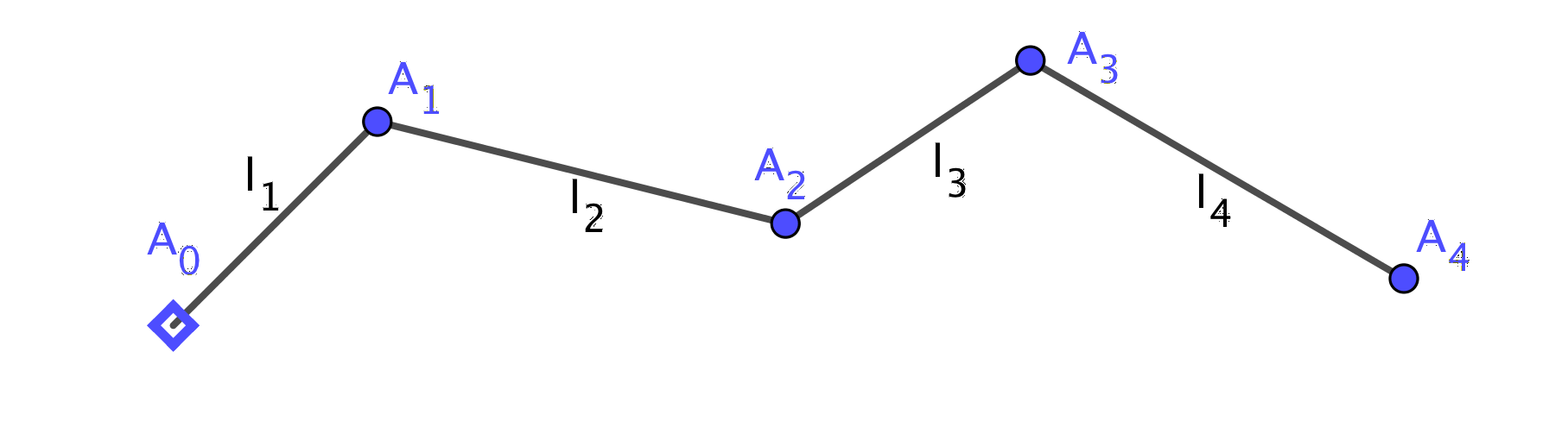
Figure 4. The snake: the canonical contravariant volume elements on its orbit space and configuration space are independent of its lengths.

Exemple 2.3.

(The snake). Consider the linkage $\mathcal{L}$ which consists of one base vertex $A_{0}$ fixed at the origin of $\mathbb{R}^{2}$ ($A_{0}=(0,0)$), $k$ movable vertices $A_{1}=(x_{1},y_{1}),\ldots,A_{k}=(x_{k},y_{k})\in\mathbb{R}^{2}$, and $k$ fixed lengths $|A_{i-1}A_{i}|=c_{i}>0$ ($i=1,\ldots,k$). Then it is easy to check that $\mathcal{O}_{\mathcal{L}}\cong\mathbb{T}^{k}$ with periodic coordinates $\theta_{i}=\arctan((y_{i}-y_{i-1})/(x_{i}-x_{i-1}))\pmod{2\pi}$, and the canonical contravariant volume element on $\mathcal{O}_{\mathcal{L}}$ is

$$\Lambda_{\mathcal{O}_{\mathcal{L}}}=\dfrac{\partial}{\partial\theta_{1}}\wedge\ldots\wedge\dfrac{\partial}{\partial\theta_{k}},$$

which does not depend on the lengths $c_{1},\ldots,c_{k}$. The configuration space $M_{\mathcal{L}}$ is isomorphic to $\mathbb{T}^{k-1}$ with periodic coordinates $\tilde{\theta}_{i}=\theta_{i+1}-\theta_{i}\pmod{2\pi}$, and its canonical contravariant volume element is (up to a sign)

$$\Lambda_{\mathcal{L}}=\dfrac{\partial}{\partial\tilde{\theta}_{1}}\wedge\ldots\wedge\dfrac{\partial}{\partial\tilde{\theta}_{k-1}}.$$

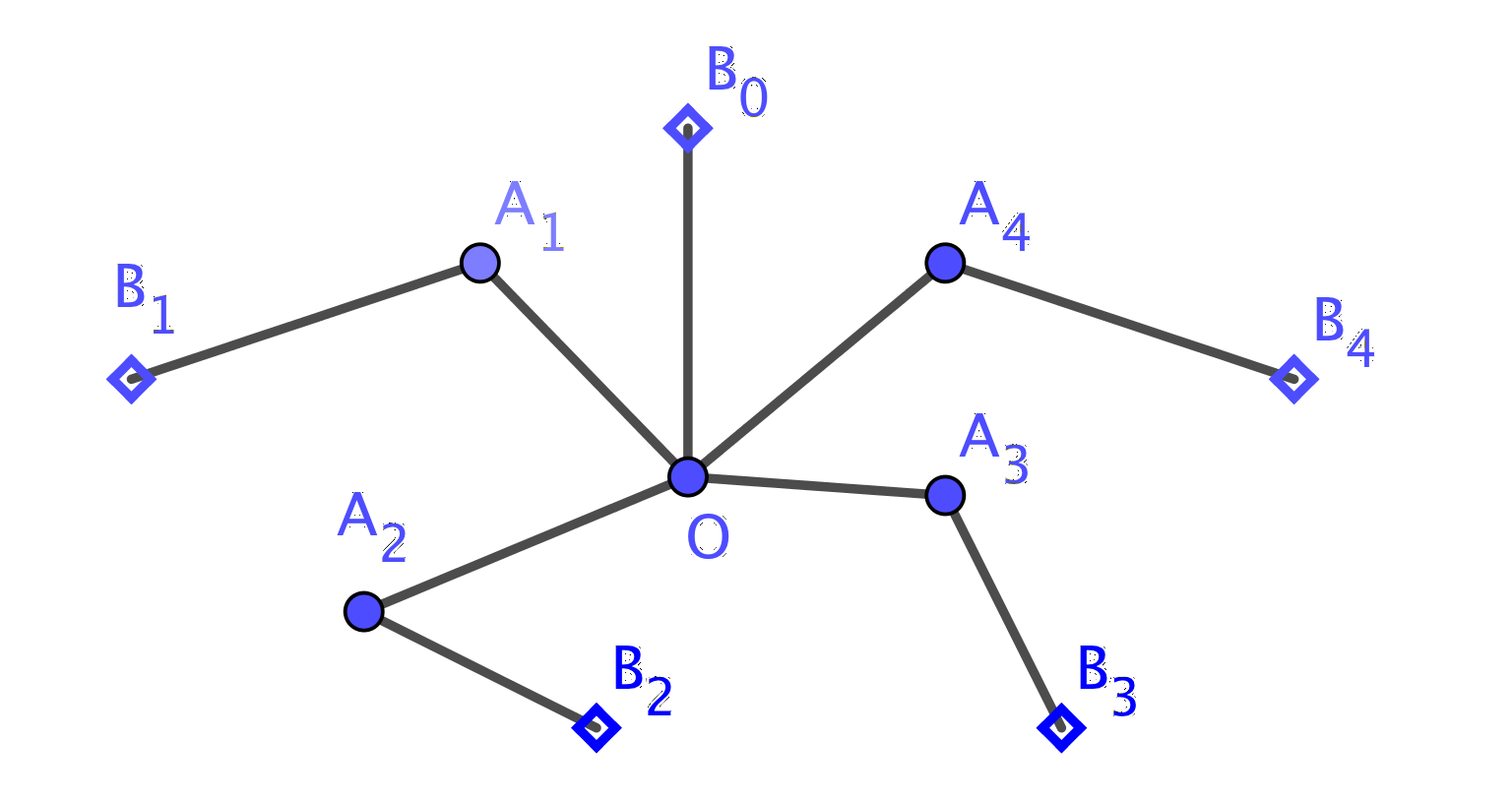
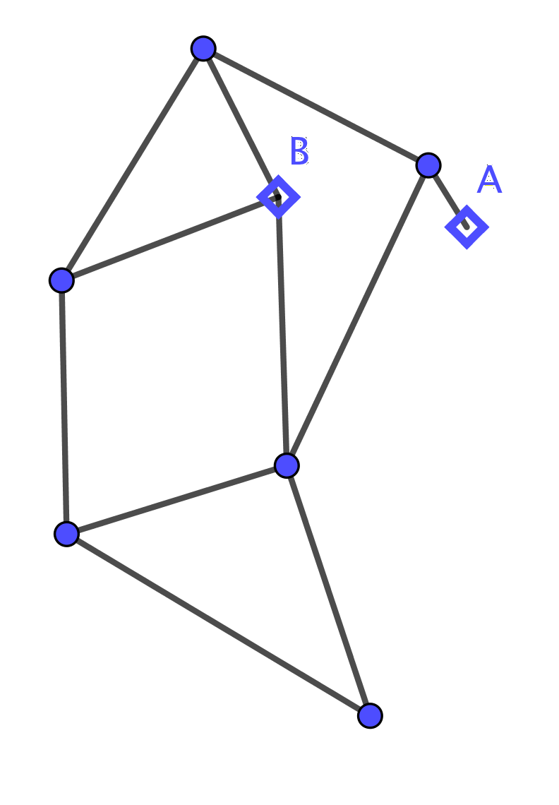
Figure 5. Left: An 1DOF spider, with a fixed “head” $B_{0}$, fixed “feet” $B_{1},\ldots,B_{n}$, “body” $O$, and “legs” $A_{i}B_{i}$ ($i=1,\ldots,n$). Right: “Strandbeest”, invented by the artist Theodorus Jansen in 1990s, which can be used as legs in mechanical animals.

Exemple 2.4.

(Curve-drawing linkages) Linkages with one degree of freedom (1DOF for short) are those whose configuration spaces have dimension 1: generically, such configuration spaces are a finite union of closed curves. A planar 1DOF linkage is also called curve-drawing linkage because, after attaching it to a plane at the fixed vertices (if there are no fixed vertices then one can choose a bar and fix its two ends without changing the configuration space of the linkage), a movable vertex on the linkage will draw an algebraic curve when the linkage moves. By a famous en the linkage moves. By a famous 1876 theorem of Kempe [17], any algebraic curve can be obtained this way by some 1DOF planar linkage. Simple modern proofs of this theorem can be found in many places; see, for example, [5, 12]. Well-known examples of 1DOF linkages include quadrangles, spiders, the Strandbeest (Figure 5), and so on. A contravariant volume element on a manifold of dimension 1 is simply a vector field. Thus, our construction shows that on the configuration space of each curve-drawing linkage there is a unique (up to orientation) natural canonical vector field. Such vector fields will be important in our construction of integrable systems on general configuration spaces of planar linkages.

Exemple 2.5.

(Zero-dimensional space). Consider a linkage $\mathcal{L}_{ABC}$ formed by a triangle $ABC$ with 3 fixed lengths (i.e., 3 bars) $|AB|=c$, $|BC|=a$, $|CA|=b$, without base points. This linkage is, of course, rigid, so its configuration space is just two points (corresponding to two possible orientations of the triangle on the plane). The contravariant volume element is just a number for each point on the configuration space. One of the numbers is twice the area of the triangle $ABC$ and the other is its opposite (the same absolute value, but with negative sign). In particular, in the degenerate case, when the three points $A,B,C$ are aligned, the contravariant volume element vanishes. If we fix $A,B$ and erase the bar $AB$ from $\mathcal{L}_{ABC}$, then it becomes another rigid linkage $\mathcal{L}_{ABC}^{\prime}$, with the same configuration space and the same contravariant volume element up to a natural isomorphism. Now add to $\mathcal{L}_{ABC}$ or $\mathcal{L}_{ABC}^{\prime}$ a vertex $D$ and a bar $CD$ with some length $|CD|=d>0$. The configuration space of the new linkage is now two circles, and the corresponding contravariant volume element is $\pm 2S\dfrac{\partial}{\partial\theta}$, where $\theta$ $\pmod{2\pi}$ is the angle formed by the vector $\overrightarrow{CD}$ with $\overrightarrow{CA}$, and $S$ is the area of the triangle $ABC$.

The above simple example illustrates the following two phenomena:

$\bullet$ (Effect of fixing a base) If $\mathcal{L}^{\prime}$ is obtained from $\mathcal{L}$ by fixing two vertices $A,B$ of a bar $AB$ and then removing that bar, where $\mathcal{L}$ is a connected linkage without base points, then not only are $M_{\mathcal{L}}$ and $M_{\mathcal{L}^{\prime}}$ naturally isomorphic, but under this isomorphism we also have $\Lambda_{\mathcal{L}}=\Lambda_{\mathcal{L}^{\prime}}$. (This fact is not surprising, because fixing $A,B$ amounts to contracting with the volume element of $SE(2)$ in the formula for $\Lambda_{\mathcal{L}}$).

$\bullet$ (Effect of homothety) If we multiply the length of every edge of a linkage $\mathcal{L}$ by a positive constant $c$, then we get a linkage $c\mathcal{L}$ homothetic to $\mathcal{L}$, and $M_{c\mathcal{L}}$ is naturally isomorphic to $M_{\mathcal{L}}$. However, under this natural isomorphism we have the following homothety formula, whose proof is a straightforward verification:

(1) $$\Lambda_{c\mathcal{L}}=c^{2(|\mathcal{E}|-(|\mathcal{V}|+|\mathcal{B}|))}\Lambda_{\mathcal{L}}$$

where $|\mathcal{V}|-|\mathcal{B}|$ is the number of movable vertices and $|\mathcal{E}|$ is the number of edges, in the case when $|\mathcal{B}|\geq 2$ (i.e., when $M_{\mathcal{L}}=\mathcal{O}_{\mathcal{L}}$) and $\mathcal{L}$ is connected. In the case when $\mathcal{B}=\emptyset$ and $\mathcal{L}$ is connected, the above formula must be modified as follows:

(2) $$\Lambda_{c\mathcal{L}}=c^{2(|\mathcal{E}|-|\mathcal{V}|+1)}\Lambda_{\mathcal{L}}$$

2.4. Nambu structures for linkages with marked diagonals

Consider a linkage $\mathcal{L}$. If two vertices $A,B$ of $\mathcal{L}$ are not connected by a bar of $\mathcal{L}$, then we say that $AB$ is a diagonal in $\mathcal{L}$. Choose a set $\mathcal{D}$ of diagonals of $\mathcal{L}$ (which may be empty) and mark the elements of $\mathcal{D}$; in this case we say that they are marked diagonals.

Given a linkage $\mathcal{L}$ with marked diagonals $\mathcal{D}=\{A_{1}B_{1},\ldots,A_{k}B_{k}\}$ ($k\geq 0$), we can define the following Nambu structure on the configuration space $M_{\mathcal{L}}$:

(3) $$\Lambda_{\mathcal{L},\mathcal{D}}=({\rm d}\mu_{1}\wedge\ldots\wedge{\rm d}\mu_{k})\!\mathbin{\hbox to6.0pt{\vrule height=0.4pt,width=5.0pt,depth=0.0pt\kern-0.4pt\vrule height=6.0pt,width=0.4pt,depth=0.0pt\hss}}\!\Lambda_{\mathcal{L}},$$

where $\mu_{i}=|A_{i}B_{i}|^{2}/2$. (When $\mathcal{D}=\emptyset$ is empty then, of course, $\Lambda_{\mathcal{L},\emptyset}=\Lambda_{\mathcal{L}}$). We will use such Nambu structures for the construction of our integrable systems.

3. Integrable systems on linkage spaces

3.1. Cross products of integrable systems

In this subsection, we present a general method for constructing new integrable systems from other integrable systems. We call this technique the cross product construction.

We begin by recalling the notion of non-Hamiltonian integrable systems ([1, 27]; for an Action-Angle Theorem in this setting, see [28]). A vector field $X$ on an $n$-dimensional manifold $M$ is called integrable if there exist $p$ vector fields $X_{1}=X$, $X_{2},\ldots,X_{p}$ and $q$ functions $F_{1},\ldots,F_{q}$ on $M$, $p+q=n$, such that $[X_{i},X_{j}]=0$ for all $i,j=1,\ldots,p$, $X_{1}\wedge\cdots\wedge X_{p}\neq 0$ almost everywhere, ${\rm d}F_{\ell}(X_{i})=0$ for all $i=1,\ldots,p$ and $\ell=1,\ldots,q$, and $\mathrm{d}F_{1}\wedge\cdots\wedge\mathrm{d}F_{q}\neq 0$ almost everywhere. Such an $n$-tuple $(X_{1},\ldots,X_{p},F_{1},\ldots,F_{q})$ is called an integrable system of type $(p,q)$.

Consider a family of smooth manifolds $M_{i}$ of dimensions $n_{i}$, where $i$ belongs to some finite index set $I$. We assume that there is another finite index set $K$ disjoint from $I$, such that for each $k\in K$ there is a nonempty subset $S_{k}\subset I$, and for each $i\in S_{k}$ there is a given smooth function $f_{i,k}:M_{i}\to\mathbb{R}$ on $M_{i}$. Moreover, we also assume that for each $i\in I$ there is an integrable non-Hamiltonian system whose functionally independent first integrals are $f_{i,k}$ for $k\in K_{i}$, where $K_{i}=\{k\in K\ |\ i\in S_{k}\}$, and whose linearly independent commuting vector fields are $X_{i,1},\ldots,X_{i,p_{i}}$. (By definition, we have $p_{i}+|K_{i}|=n_{i}$).

Consider now the diagonal manifold

(4) $$M=\Big{\{}{\bf x}=(x_{i})\in\prod_{i\in I}M_{i}\ \Big{|}\ f_{ik}(x_{i})=f_{jk}(x_{j})\ \forall i,j\in I,\ \forall k\in S_{i}\cap S_{j}\subset K\Big{\}}.$$

Denote by $\pi_{j}:\prod_{i\in I}M_{i}\to M_{j}$ the projection maps. By abuse of notation, we denote the restriction of $\pi_{j}$ to $M$ again by $\pi_{j}$, $j\in I$. We assume that the functions $\pi_{i}^{*}f_{ik}-\pi_{j}^{*}f_{jk}$ ($k\in S_{i}\cap S_{j}$) have linearly independent differentials on $M$, except at the points satisfying the obvious relations of the type $\pi_{i}^{*}f_{ik}-\pi_{j}^{*}f_{jk}=(\pi_{i}^{*}f_{ik}-\pi_{\ell}^{*}f_{\ell k})+(\pi_{\ell}^{*}f_{\ell k}-\pi_{j}^{*}f_{jk})$; therefore, $M$ is a smooth manifold of dimension $\dim M=\sum_{i\in I}n_{i}-\sum_{k\in K}(|S_{k}|-1)=\sum_{i\in I}n_{i}-\sum_{k\in K}|S_{k}|+|K|$ (because each index $k\in K$ creates $|S_{k}|-1$ independent equations). Notice that $\sum_{k\in K}|S_{k}|$ is the total number of functions $f_{ik}$ and that this number equals $\sum_{i\in I}(n_{i}-p_{i})$, because for each $i$ we have exactly $|K_{i}|=n_{i}-p_{i}$ functions. Therefore,

(5) $$\dim M=|K|+\sum_{i\in I}p_{i}.$$

Denote by $\widehat{X}_{i,j}$ the horizontal lift of $X_{i,j}$ to $\prod_{i\in I}M_{i}$ (for each $i\in I$ and each $j\leq p_{i}$). In other words, $\widehat{X}_{i,j}$ is the unique vector field on $\prod_{i}M_{i}$ whose projections by $\pi_{j}$ ($j\neq i$) are trivial and whose projection by $\pi_{i}$ is $X_{i,j}$. Obviously, the vector fields $\widehat{X}_{i,j}$ commute on $\prod_{i\in I}M_{i}$. Moreover, they admit the pull-backs of the functions $f_{ik}$ as common first integrals. Hence, they also admit the functions $\pi_{i}^{*}f_{ik}-\pi_{j}^{*}f_{jk}$ as first integrals and are, therefore, tangent to $M$.

For each $k\in K$, define $F_{k}:M\to\mathbb{R}$ by

(6) $$F_{k}({\bf x})=f_{ik}(\pi(x_{i}))\quad\text{for some}\quad i\in S_{k}.$$

It is immediate from the definition of $M$ that $F_{k}$ is well-defined. Moreover, these functions $F_{k}$ are common first integrals of the commuting vector fields $X_{i,j}$ ($i\in I,j\leq p_{i}$). Notice that the number of vector fields $X_{i,j}$ is $\sum_{i\in I}p_{i}$, the number of functions $F_{k}$ is $|K|$, and $|K|+\sum_{i\in I}p_{i}$ is exactly the dimension of $M$ (see (5)). Thus, we immediately obtain the following result.

Theorem 3.1.

With the above notations and assumptions, on the diagonal manifold $M$ of dimension $|K|+\sum_{i\in I}p_{i}$ we have an integrable system of type $\left(\sum_{i\in I}p_{i},|K|\right)$, consisting of $\sum_{i\in I}p_{i}$ commuting vector fields $\widehat{X}_{i,j}$ ($i\in I,j\leq p_{i}$) and $|K|$ first integrals $F_{k}$ ($k\in K$) given by (6).

The above constructed integrable system on $M$ is called the cross product of the corresponding integrable systems on $M_{i},i\in I$.

3.2. Multi-Nambu integrable systems

Consider now the following special case of the general cross product construction in the previous subsection.

Assume that for each $i\in I$, the set $\{f_{i,k}\mid k\in K_{i}\}$ ($K_{i}=\{k\in K\mid i\in S_{k}\}$), of functionally independent functions on $M_{i}$ has exactly $n_{i}-1$ elements, where $n_{i}=\dim M_{i}$ and, moreover, each $M_{i}$ admits a Nambu structure $\Lambda_{i}$ of top order, i.e., a $n_{i}$-vector field on $M_{i}$. (In practice, $\Lambda_{i}$ is often the dual of a volume form on $M_{i}$, though the construction still works if $\Lambda_{i}$ has singular points.) Then, for each $i\in I$, define the Nambu vector field $X_{i}$ on $M_{i}$ by the following contraction formula:

(7) $$X_{i}=\left(\wedge_{k\in K_{i}}{\rm d}f_{i,k}\right)\!\mathbin{\hbox to6.0pt{\vrule height=0.4pt,width=5.0pt,depth=0.0pt\kern-0.4pt\vrule height=6.0pt,width=0.4pt,depth=0.0pt\hss}}\!\Lambda_{i}.$$

(Choose an ordering on $K_{i}=\{k\in K\mid i\in S_{k}\}$ to fix the sign of $\wedge_{k\in K_{i}}{\rm d}f_{i,k}$). Clearly, $X_{i}$ admits $n_{i}-1$ first integrals $f_{i,k}$ ($k\in K_{i}$), since $|K_{i}|=n_{i}-1$, and hence $X_{i}$ is a completely integrable vector field on $M_{i}$. In other words, on each $M_{i}$ we have an integrable system $(X_{i},f_{i,k})$ of type $(1,n_{i}-1)$. So, in the notation of the previous subsection, we have $p_{i}=1$ and $\sum_{i\in I}p_{i}=|I|$. Thus we get:

Corollary 3.2.

With the above notations and assumptions of this subsection, on the diagonal manifold $M$ of dimension $|I|+|K|$ we have an integrable system of type $(|I|,|K|)$, consisting of $|I|$ commuting vector fields $\widehat{X}_{i}$ ($i\in I$) and $|K|$ first integrals $F_{k}$ ($k\in K$).

In view of this construction, we call the systems obtained in the corollary above multi-Nambu integrable systems.

Remark 3.3.

(Separation of variables and symplectization).

i) The construction above not only gives integrable systems, but also a kind of separation of variables for such systems: the separated variables are on the different spaces $M_{i}$ ($i\in I$). In classical mechanics, a Hamiltonian system admitting a complete separation of variables, in the sense of Hamilton-Jacobi theory, is automatically integrable. Our systems are a special case of this general idea, even though, a priori, there is no natural (pre)symplectic or Poisson structure which turns them into Hamiltonian systems.

ii) An exception is the case when $\dim M_{i}=2$, for every $i\in I$, and the Nambu structure $\Lambda_{i}$ on $M_{i}$ is non-degenerate, i.e., it is dual to a volume form $\omega_{i}$ on $M_{i}$. In dimension 2, a volume form is the same as a symplectic form. In this situation we can pull back every $\omega_{i}$ and take their sum to form a presymplectic form

$$\omega=\sum_{i\in I}\pi_{i}^{*}\omega_{i}$$

on the diagonal manifold $M$. Thus we obtain a presymplectic manifold $(M,\omega)$ together with an integrable Hamiltonian system $(\widehat{X}_{i}\ (i\in I),F_{k}\ (k\in K))$. Each vector field $\widehat{X}_{i}$ is Hamiltonian: $\widehat{X}_{i}\!\mathbin{\hbox to6.0pt{\vrule height=0.4pt,width=5.0pt,depth=0.0pt\kern-0.4pt\vrule height=6.0pt,width=0.4pt,depth=0.0pt\hss}}\!\omega=-{\rm d}F_{k}$, where $k\in K$ is the only index in $S_{i}$ (i.e, there is only one function $f_{ik}$ on $M_{i}$). The rank of $\omega$ at a generic point on $M$ is $2|K|$ in this case.

iii) If $\dim M_{i}\geq 3$, then even if $|I|=1$, there is no natural way to turn the Nambu vector field $X_{i}$ on $M_{i}$ into a Hamiltonian vector field (with respect to a presymplectic, Poisson, or Dirac structure). The problem is that, in Nambu mechanics, we have $n-1$ functions which play equally important roles in the definition of the Nambu vector field, while in Hamiltonian mechanics we have just one function (the energy function). In order to turn a Nambu vector field into a Hamiltonian vector field, one needs to treat these functions differently and declare that among the $n-1$ function there is a special one which is more important than the other functions. Of course, this can be done. For example, a Nambu vector field $X=({\rm d}F_{1}\wedge\ldots\wedge{\rm d}F_{n-1})\!\mathbin{\hbox to6.0pt{\vrule height=0.4pt,width=5.0pt,depth=0.0pt\kern-0.4pt\vrule height=6.0pt,width=0.4pt,depth=0.0pt\hss}}\!\Lambda$, where $\Lambda$ is a Nambu structure of order $n$ on a manifold, may be viewed as a Hamiltonian vector field given by $F_{1}$ with respect to the Poisson structure $\Pi=({\rm d}F_{2}\wedge\ldots\wedge{\rm d}F_{n-1})\!\mathbin{\hbox to6.0pt{\vrule height=0.4pt,width=5.0pt,depth=0.0pt\kern-0.4pt\vrule height=6.0pt,width=0.4pt,depth=0.0pt\hss}}\!\Lambda$ of rank 2. Nevertheless, this is not very natural, especially in view of the diagonal construction.

iv) Moreover, there is no natural way to lift multi-vector fields from $M_{i}$ to the diagonal manifold $M$ (the horizontal lifting that we used for our vector fields does not work here because the result is not tangent to $M$). Thus, even if the $M_{i}$ are equipped with Poisson structures, $M$ is still not Poisson. We cannot even lift Nambu structures $\Lambda_{i}$ from $M_{i}$ to $M$. So the Nambu structures in a multi-Nambu integrable system are not Nambu structures on the ambient manifold, only on its projected components.

3.3. Decomposition of linkages and integrable systems

We apply now the constructions in the previous subsections to the configuration spaces of planar linkages.

Consider a planar linkage $\mathcal{L}=(\mathcal{V},\mathcal{E},\ell)$ without base points. (Recall that any non-trivial linkage with base points is equivalent to some linkage without base points, configuration-wise). Choose a set $\mathcal{D}$ of diagonals of $\mathcal{L}$ such that $\mathcal{D}$ decomposes $\mathcal{L}$ into an acyclic semi-rigid connected sum of a family of non-empty sublinkages $\mathcal{L}_{i}=(\mathcal{V}_{i},\mathcal{E}_{i},\ell_{i})$ ($i\in I$) with their corresponding sets $\mathcal{D}_{i}$ of marked diagonals. This means that the following conditions are satisfied:

• For each $i\in I$, denote by $\mathcal{V}_{i}$ the set of vertices of $\mathcal{L}_{i}$. Then $\mathcal{L}_{i}=(\mathcal{V}_{i},\mathcal{E}_{i},\ell_{i})$ is the sublinkage of $\mathcal{L}$ generated by $\mathcal{V}_{i}$. This means that $\mathcal{E}_{i}$ is the subset of $\mathcal{E}$ consisting of all edges of $\mathcal{L}$ such that all of their vertices belong to $\mathcal{V}_{i}$; likewise, $\ell_{i}$ and $\mathcal{D}_{i}$ are also defined in a natural way. (The diagonals in the family $\mathcal{D}_{i}$ are the elements of $\mathcal{D}$ whose vertices belong to $\mathcal{V}_{i}$.)

• $\mathcal{V}=\cup_{i\in I}\mathcal{V}_{i}$, $\mathcal{E}=\cup_{i\in I}\mathcal{E}_{i}$, and $\mathcal{D}=\cup_{i\in I}\mathcal{D}_{i}$.

• There is a family $\mathcal{J}_{k}$ ($k\in K$) of sublinkages of $\mathcal{L}$, which are called joints for the sublinkages $\mathcal{L}_{i}$, in the following sense: if $\mathcal{L}_{i}\cap\mathcal{L}_{j}\neq\emptyset$ for $i,j\in I$, then there is a $k\in K$ such that $\mathcal{L}_{i}\cap\mathcal{L}_{j}=\mathcal{J}_{k}$. (It may happen that more than two sublinkges in the family $\mathcal{L}_{i}$ ($i\in I$) share the same joint; see Figure 6).

• Every marked diagonal is a diagonal of a joint: for any $VW\in\mathcal{D}$ there is a joint $\mathcal{J}_{k}$ such that $V,W$ are vertices of $\mathcal{J}_{k}$.

• The joints are disjoint: if $k_{1}\neq k_{2}$ then $\mathcal{J}_{k_{1}}$ and $\mathcal{J}_{k_{2}}$ don’t have any common vertex.

• Semi-rigidity: For each $k\in K$, $\mathcal{J}_{k}$ has at least $2$ vertices. If we fix the lengths of the marked diagonals (from the family $\mathcal{D}$) whose vertices lie in $\mathcal{J}_{k}$ then $\mathcal{J}_{k}$ becomes rigid, i.e., its configuration space becomes just one point (if not empty) once these diagonal lengths are fixed.

• Acyclicity: Consider the graph whose vertices are the elements of the index sets $I$ and $K$ (of course, these two index sets are assumed to be disjoint) and whose edges are the couples $(i,k)\in I\times K$ (connecting the vertex $i$ to the vertex $k$) such that the sublinkage $\mathcal{L}_{i}$ contains the joint $\mathcal{J}_{k}$. Then this graph is a tree (i.e., it has no cycles).

Figure 6. Example of a connected sum with two joints and two marked diagonals $AF$ and $OP$: four sublinkages share the same joint $\{A,F\}$ and three sublinkages share the same joint $\{O,P\}$.

Definition 3.4.

With the above notations and under the above conditions, we say that $(\mathcal{L},\mathcal{D})$ is the acyclic semi-rigid connected sum of its sublinkages with marked diagonals $(\mathcal{L}_{i},\mathcal{D}_{i})$ ($i\in I$).

Theorem 3.5.

(i) With the above notations, assume that $(\mathcal{L},\mathcal{D})$ is the acyclic semi-rigid connected sum of the family $(\mathcal{L}_{i},\mathcal{D}_{i})$ ($i\in I$). Assume that the diagonal square length functions $\mu_{VW}=\ell(VW)^{2}/2$ ($VW\in\mathcal{D}$) are functionally independent almost everywhere on the configuration space $M_{\mathcal{L}}$, and that for every $i\in I$ the number of elements in $\mathcal{D}_{i}$ is strictly less than the dimension $\dim M_{\mathcal{L}_{i}}$ of the configuration space of $\mathcal{L}_{i}$. Then $M_{\mathcal{L}}$ is the cross product of the family $M_{\mathcal{L}_{i}}$ with respect to the marked square length functions:

$$M_{\mathcal{L}}\cong\Big{\{}\mathbf{x}=(x_{i})\in\prod_{i\in I}M_{\mathcal{L}_{i}}\ |\ \mu_{d}(x_{i})=\mu_{d}(x_{j})\ \forall i,j\in I,\ \forall d\in\mathcal{D}_{i}\cap\mathcal{D}_{j}\Big{\}}.$$

In particular, we have

$$\dim M_{\mathcal{L}}=\sum_{i\in I}(\dim M_{\mathcal{L}_{i}}-|\mathcal{D}_{i}|)+|\mathcal{D}|.$$

(ii) Assume, moreover, that on each configuration space $M_{\mathcal{L}_{i}}$ we have an integrable system of type $(p_{i},q_{i})$, where $q_{i}=|\mathcal{D}_{i}|$ and $p_{i}=\dim M_{\mathcal{L}_{i}}-q_{i}$, given by $p_{i}$ commuting vector fields $X_{i,1},\ldots,X_{i,p_{i}}$ and $|\mathcal{D}_{i}|$ diagonal squared length functions $\mu_{d}$ ($d\in\mathcal{D}_{i}$) which serve as first integrals for the system. Then by the method of cross product construction we get an integrable system of type $\left(\sum_{i\in I}p_{i},|\mathcal{D}|\right)$ on $M_{\mathcal{L}}$ given by the vector fields $\widehat{X}_{i,j}$ (which are horizontal liftings of the vector fields $X_{i,j}$, $i\in I$, $j\leq p_{i}$) and diagonal squared length functions $\mu_{d}$ ($d\in\mathcal{D}$).

(iii) In particular, if $\dim M_{\mathcal{L}_{i}}-|\mathcal{D}_{i}|=1$ for every $i\in I$, then on each $\dim M_{\mathcal{L}_{i}}$ we have an integrable system of type $(1,|\mathcal{D}_{i}|)$ given by $|\mathcal{D}_{i}|$ marked diagonal square length functions and the Nambu vector field $X_{i}$ given by formula (7) with respect to these functions and the natural contravariant volume element on $\dim M_{\mathcal{L}_{i}}$. Consequently, in this case on $M_{\mathcal{L}}$ we have a multi-Nambu integrable system of type $(|I|,|\mathcal{D}|)$.

The proof of the above theorem is straightforward. In assertion (i), the semi-rigidity and the acyclicity conditions ensure that, for each point $(x_{i})\in\prod_{i}M_{\mathcal{L}_{i}}$ satisfying the “equal common lengths” constraints, we can glue the configurations $x_{i}$ together along the joints to create a configuration $x\in M_{\mathcal{L}}$, in a unique way up to isometries. Assertions (ii) and (iii) follow immediately from of assertion (i), Theorem 3.1, and Corollary 3.2.

Exemple 3.6.

The case of $n$-gons. Denote by $(A_{1},...,A_{n})$ the consecutive vertices of an $n$-gon. The configuration space $M_{\mathcal{L}}$ in this case has $2(n-2)-(n-1)=n-3$ dimensions.

If $n$ is even, we can divide the $n$-gon $(A_{1}\dots A_{n})$ into $(n/2)-1$ quadrangles by adding $(n/2)-2$ diagonals to the linkage; for example, $A_{1}A_{3},A_{1}A_{5},\ldots,A_{1}A_{2n-1}$. Each quadrangle may be viewed as a curve-drawing linkage and thus produces one vector field. So we have an integrable system of type $\big{(}(n/2)-1,(n/2)-2\big{)}$, i.e., with $(n/2)-1$ commuting vector fields and $(n/2)-2$ common first integrals.

If $n$ is odd, divide the $n$-gon $(A_{1}\dots A_{n})$ into $(n-3)/2-1$ quadrangles plus one triangle by adding $(n-3)/2$ diagonals to the linkage; for example, $A_{1}A_{3},A_{1}A_{5},\ldots,A_{1}A_{2n-1}$. So we get an integrable system of type $((n-3)/2,(n-3)/2)$.

Remark 3.7.

i) In assertion (iii) of Theorem 3.5, once the lengths of the marked diagonals are fixed, the sublinkages $\mathcal{L}_{i}$ become curve-drawing linkages (i.e, linkages whose configuration spaces are 1-dimensional). This shows that curve-drawing linkages play an important role in the construction of integrable systems on the configuration spaces of more general planar linkages.

ii) In a sense, the above construction is quite similar to the construction of bending flows by Kapovich and Millson [15] for obtaining integrable systems on configuration spaces of 3D polygons.

iii) The case when then dimension of $M_{\mathcal{L}_{i}}$ is equal to (instead of being greater than) the number of marked diagonals in ${\mathcal{L}_{i}}$ for some $i\in I$ is excluded in Theorem 3.5 for simplicity. However, this case can, in fact, be treated similarly. In order to address this case, we have to work on the level of orbit spaces instead of configuration spaces, so it is a bit more complicated. Some components ${\mathcal{L}_{i}}$ for which the number of marked diagonals is equal to $\dim\mathcal{L}_{i}$ still give rise to a non-trivial (and periodic) vector field in the final integrable system on $M_{\mathcal{L}}$. For example, see the case of the snake (Example 2.3), which is cut into pieces. Each piece has 0-dimensional configuration space, but the configuration space of the snake is a torus with natural rotational commuting vector fields.

The case when a joint $J_{k}$ consists of just one point is also excluded in Theorem 3.5 for simplicity. However, this case can also be treated similarly. Such a $J_{k}$ increases the difference $M_{\mathcal{L}}-\sum_{i}\dim M_{\mathcal{L}_{i}}$ and creates additional rotational vector fields on $M_{\mathcal{L}}$.

Likewise, the case with base points, also excluded in Theorem 3.5, can also be treated similarly; just put all the base points in one component.

iv) There is an obvious method to create integrable systems on configuration spaces, which works for any planar linkage. If the dimension of the configuration space $M_{\mathcal{L}}$ is $n$, then just mark $n-1$ diagonals whose length functions are independent on $M_{\mathcal{L}}$. Then, together with the contravariant volume element on $M_{\mathcal{L}}$, we immediately get a Nambu integrable system of type $(1,n-1)$ whose first integrals are squared length functions of the marked diagonals and whose vector field is given by formula (7). However, such “obvious” systems have just one vector field each, so if we want to obtain systems with more vector fields using the cross product method, we have to decompose the linkage $\mathcal{L}$ into many components $\mathcal{L}_{i}$, the more, the better.

Figure 7. Example of an indecomposable 3DOF linkage.

v) A natural question arises: given a planar linkage $\mathcal{L}$, what is the maximal number $|I|$ of components $\mathcal{L}_{i}$ ($i\in I$) in a decomposition of $\mathcal{L}$ into acyclic semi-rigid connected sums (with any choice of marked diagonals, such that the dimension of the configuration space of each $\mathcal{L}_{i}$ is strictly greater than the number of marked diagonals in it)? If this maximal number is 1, then we say that $\mathcal{L}$ is indecomposable. Figure 7 is an example of a 3DOF indecomposable linkage (i.e., the configuration space has dimension 3).

vi) In general, it is clear that the number of components in a “valid” acyclic semi-rigid connected sum (“valid” means that $\dim M_{\mathcal{L}_{i}}$ is strictly greater than the number of marked diagonals in $\mathcal{L}_{i}$) cannot be greater than $(|\mathcal{V}|-1)/2$, where $|\mathcal{V}|$ is the number of vertices of the linkage $\mathcal{L}$, because each time one adds a new component to such an acyclic semi-rigid connected sum, one needs to add at least 2 new vertices, and the first component has at least 3 vertices. An example where the maximal number $(|\mathcal{V}|-1)/2$ of components is achieved is shown in Figure 8. The linkage $\mathcal{L}$ has 7 vertices, the configuration space has 4 dimensions, and the following decomposition of $\mathcal{L}$ into 3 components is valid: $\mathcal{L}_{1}$ is generated by $\{A,B,G\}$, $\mathcal{L}_{2}$ is generated by $\{B,C,F,G\}$, $\mathcal{L}_{3}$ is generated by $\{C,D,E,F\}$, and the only marked diagonal is $CF$. So, on this 4-dimensional configuration space, we have an integrable system of type $(3,1)$, with three commuting vector fields and one common first integral.

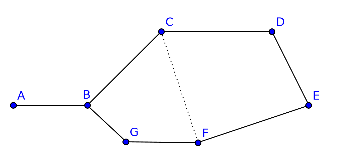
Figure 8. A linkage which can be decomposed into 3 “elementary” components.

4. Some final remarks and open problems

4.1. Bott-Morse theory and graph-manifolds

The topology of configuration spaces of planar linkages has been extensively studied using mostly Morse theory, see, e.g., [5, 6, 9, 10, 11, 12, 13, 14] and references therein. However, in general, the square length functions that we use in this paper are not Morse functions, but rather Bott-Morse functions: their singular points are not isolated but form submanifolds and are transversally non-degenerate with respect to these submanifolds. So the idea of using Bott-Morse functions (instead of just Morse functions) for the study of the topology of linkage spaces is very natural.

At least in the case of linkages with 3-dimensional spaces which admit integrable systems of type (2,1), this idea works very well: the situation is then very similar to Fomenko’s topological theory of 2-degree-of-freedom integrable Hamiltonian systems restricted to 3-dimensional isoenergy manifolds [7]. One of the main observations made by Fomenko is that, due to the Bott-Morse nature of the first integral, the 3-dimensional manifolds in question must be graph-manifolds, i.e., they can be cut into pieces which are direct products of $S^{1}$ with 2-dimensional surfaces with boundary. The class of graph-manifolds has been introduced by Waldhausen [25] in 1967 and is a very well-understood class of 3-manifolds. (Incidentally, according to the Thurston-Perelman geometrization program, this class coincides with the class of 3-manifolds whose Gromov norm vanishes).

For example, consider the configuration space $M_{\ell}$ of hexagons $A_{1}A_{2}A_{3}A_{4}A_{5}A_{6}$ with fixed edge lengths $|A_{i}A_{i+1}|=\ell_{i}$ ($i=1,\ldots,6$, $A_{7}=A_{1}$). We assume that the lenghths are generic and that $M_{\ell}$ is not empty. Denote by $d=A_{1}A_{4}$ the length of the diagonal $A_{1}A_{4}$. Then $d$ is a function on $M_{\ell}$, which is not smooth; however, $\mu=d^{2}/2$ is smooth and is a Bott-Morse function on $M_{\ell}$, whose singular points form circles. It follows immediately that $M_{\ell}$ is a graph-manifold. To study the topology of $M_{\ell}$ more carefully, one needs to investigate in detail the singularities of $\mu$. For example, assume (without loss of generality for the topology of $M_{\ell}$) that $\ell_{1}\leq\ell_{2}\leq\ell_{3}\leq\ell_{4}\leq\ell_{5}\leq\ell_{6}$. Then the possible critical values of $d$ are:

• the maximal value: $\ell_{1}+\ell_{2}+\ell_{3}$,

• possible saddle values: $\ell_{1}+\ell_{2}-\ell_{3}$ (if this value is positive), $\ell_{3}+\ell_{2}-\ell_{1}$, $\ell_{3}+\ell_{1}-\ell_{2}$, $\ell_{4}+\ell_{5}-\ell_{6}$ (if this value is positive), $\ell_{6}+\ell_{5}-\ell_{4}$, $\ell_{6}+\ell_{4}-\ell_{5}$;

• the minimal value is either 0 (if both $\ell_{1}+\ell_{1}-\ell_{3}$ and $\ell_{4}+\ell_{5}-\ell_{6}$ are positive) or $\max(\ell_{3}-\ell_{1}-\ell_{2},\ell_{6}-\ell_{4}-\ell_{5})$ (if this value is positive).

Then one describes the level sets at and near these critical values, the 1-cycles on them, and so on, to recover a long list of all possibilities (see [14]). This would be an interesting exercise for graduate students.

4.2. Integrable systems on more general linkage spaces

In this paper, we used our decomposition and the cross product method to construct integrable systems on the configuration spaces of planar linkages. It it clear that our method can be applied, in a straightforward way, to other classes of linkages, including spherical linkages, 3D linkages, and higher-dimensional linkages. (See [18] for a general theory of linkage designs, including spherical linkages and spatial linkages). In particular, according to our method, the class of configuration spaces of 3D linkages admitting interesting natural integrable systems is much bigger than the class of 3D polygon spaces studied by Kapovich-Millson [15] and others. As far as we know, this bigger class has not yet been explored and it is an interesting subject of study, with potential applications in robotics.

4.3. Singularities of integrable systems on linkage spaces

Singularities of integrable Hamiltonian systems have been studied by many authors. More recently, there has been interest in formulating a theory of singularities of integrable non-Hamiltonian systems (see [27] and references therein). A detailed study of singularities of concrete integrable systems on configuration spaces of planar linkages would help the development of this theory.

4.4. Commuting flows for 2DOF components

In this paper, in the construction of integrable systems on configuration spaces, we only used components which are 1DOF (i.e., curve-drawing), once the lengths of the marked diagonals are fixed. What about 2DOF components? Can they be used effectively? In particular, is there any natural way to construct a pair of independent commuting vector fields on the configuration spaces of pentagons, for example? These configuration spaces are closed surfaces and it is known that on such surfaces there exist $\mathbb{R}^{2}$-actions with nondegenerate singularities (see, e.g., [21]). The question is hence how to construct such $\mathbb{R}^{2}$-actions in a natural way on 2-dimensional moduli spaces of planar linkages. What about components with more degrees of freedom (once the lengths of the marked diagonals are fixed).

References

- [1] O.I. Bogoyavlenskij, A concept of integrability of dynamical systems, C. R. Math. Rep. Acad. Sci. Canada, 18 (1996), 163–168.
- [2] O.I. Bogoyavlenskij, Extended integrability and bi-hamiltonian systems, Comm. Math. Phys., 196(1) (1998), 19–51.
- [3] D. Bouloc, Singular fibers of the bending flows on the moduli space of 3D polygons, Journal of Symplectic Geometry, 16(3) (2018), 585–629.
- [4] J.-P. Dufour, N.T Zung, Poisson Structures and Their Normal Forms, Progress in Mathematics Vol. 242, Birkhäuser, 2015.
- [5] M. Farber, An Invitation to Topological Robotics, Zürich Lectures in Advanced Mathematics, European Mathematical Society Publishing House, 2008.
- [6] M. Farber, D. Schütz, Homology of planar polygon spaces, Geom. Dedicata, 125 (2007), 75–92.
- [7] A.T. Fomenko, Symplectic topology of completely integrable Hamiltonian systems, Russian Math. Surveys, 44(1) (1989), 181–219.
- [8] C.G. Gibson, J.M. Selig, Movable hinged spherical quadrilaterals, I Über sphärische Gelenkenvierecke: the configuraion space, II singularities and reduction, Mechanism and Machine Theory, 23(1) (1988), 13–18; 19–24.
- [9] C.G. Gibson, D. Marsh, On the linkage varieties of Watt 6-bar mechanisms, I Basic geometry, II The possible reductions, III Topology of the real varieties, Mechanism and Machine Theory, 24 (1989), 106–113; 115–121; 123–126.
- [10] J.-C. Hausmann, A. Knutson, Polygon spaces and Grassmannians, Enseign. Math.(2), 43(1-2) (1997), 173–198.
- [11] J.-C. Hausmann, A. Knutson, Cohomology rings of polygon spaces, Ann. Inst. Fourier (Grenoble), 48 (1988), 281–321.
- [12] D. Jordan, M. Steiner, Configuration spaces of mechanical linkages, Discrete Comput. Geom., 22 (1999), 297–315.
- [13] Y. Kamiyama, S. Tsukuda, The Euler characteristic of the configuration space of planar spidery linkages, Algebr. Geom. Topol., 14(6) (2014), 3659–3688.
- [14] M. Kapovich, J. Millson, On the moduli space of polygons in the Euclidean plane, J. Diff. Geom., 42(2) (1995), 430–464.
- [15] M. Kapovich, J. Millson, The symplectic geometry of polygons in Euclidean space, J. Diff. Geom., 44(3) (1996), 479–513.
- [16] M. Kapovich, J. Millson, Universality theorems for configuration spaces of planar linkages, Topology, 41 (2002), 1051–1107.
- [17] A.B. Kempe, On a general method of describing plane curves of the th degree by linkwork, Proc. London Math. Soc., VII, 102 (1876), 213–216.
- [18] J.M. McCarthy, G.S. Soh, Geometric Design of Linkages, second edition, Springer, 2011.
- [19] A. Klyachko, Spatial polygons and stable configurations of points on the projective line, in Algebraic Geometry and Its Applications, Proceedings of the 8th Algebraic Geometry Conference, Yaroslavl’ 1992, (A. Tikhomirov and A. Tyurin, eds.), Vieweg, Braunschweig, 1994, pp. 67–84.
- [20] T.H. Minh, N.T. Zung, Commuting foliations, Regular and Chaotic Dynamics, 18(6) (2013), 608–622.
- [21] N.V. Minh, N.T. Zung, Geometry of nondegenerate -actions on -manifolds, J. Math. Soc. Japan, 66(3) (2014), 839–894.
- [22] Y. Nambu, Generalized Hamiltonian dynamics, Phys. Rev. D., 7(8) (1973), 5405–5412.
- [23] B. Servatius, O. Shai, W. Whiteley, Combinatorial characterization of the Assur graphs from engineering, European J. Combin., 31(4) (2010), 1091–1104.
- [24] W. Thurston, Shapes of polyhedra, Preprint 1987.
- [25] F. Waldhausen, Eine Klasse von 3-dimensionalen Mannigfaltigkeiten, I & II. Inventiones Mathematicae, 3 (4): 308–333 and 4 (2): 87–117 (1967).
- [26] J. Zhao, Z. Feng, N. Ma, F. Chu, Design of special planar linkages, Springer Tracks in Mechanical Engineering, 2014.
- [27] N.T. Zung, Geometry of integrable non-Hamiltonian systems, in Geometry and Dynamics of Integrable Systems, Advanced Courses in Mathematics, CRM Barcelona, pp. 85–140. Birkhäuser/Springer, 2016.
- [28] N.T. Zung, A conceptual approach to the problem of action-angle variables, Arch. Rat. Mech. Anal., 229(2) (2018), 789–833.