New Perspectives on the Schrödinger-Pauli Theory of Electrons: Part II: Application to the Triplet State of a Quantum Dot in a Magnetic Field

Abstract

The Schrödinger-Pauli theory of electrons in the presence of a static electromagnetic field can be described from the perspective of the individual electron via its equation of motion or ‘Quantal Newtonian’ first law. The law is in terms of ‘classical’ fields whose sources are quantum-mechanical expectation values of Hermitian operators taken with respect to the wave function. The law states that the sum of the external and internal fields experienced by each electron vanishes. The external field is the sum of the binding electrostatic and Lorentz fields. The internal field is the sum of fields representative of properties of the system: electron correlations due to the Pauli exclusion principle and Coulomb repulsion; the electron density; kinetic effects; the current density. Thus, the internal field is a sum of the electron-interaction, differential density, kinetic, and internal magnetic fields. The energy can be expressed in integral virial form in terms of these fields. Via this perspective, the Schrödinger-Pauli equation can be written in a generalized form which then shows it to be intrinsically self-consistent. This new perspective is explicated by application to the triplet $2^{3}S$ state of a $2$-D $2$-electron quantum dot in a magnetic field. The quantal sources of the density; the paramagnetic, diamagnetic, and magnetization current densities; pair-correlation density; the Fermi-Coulomb hole charge; and the single-particle density matrix are obtained, and from them the corresponding fields determined. The fields are shown to satisfy the ‘Quantal Newtonian’ first law. The components of the energy too are determined from these fields. Finally, the example is employed to demonstrate the intrinsic self-consistent nature of the Schrödinger-Pauli equation.

I Introduction

The Schrödinger-Pauli theory 1 is a description of a system of $N$ electrons in the presence of an external electrostatic binding field ${\boldsymbol{\cal{E}}}({\bf{r}})=-{\boldsymbol{\nabla}}v({\bf{r}})/e$ and a magnetostatic field ${\boldsymbol{\cal{B}}}({\bf{r}})={\boldsymbol{\nabla}}\times{\bf{A}}({\bf{r}})$, where $v({\bf{r}})$ and ${\bf{A}}({\bf{r}})$ are scalar and vector potentials. In the theory the interaction of the magnetic field with both the orbital and spin angular momentum is explicitly considered. The stationary-state Schrödinger-Pauli differential equation is (charge of electron $-e$)

$$\bigg{[}\frac{1}{2m}\sum_{k}\big{(}\hat{\bf{p}}_{k}+\frac{e}{c}{\bf{A}}({\bf{r}}_{k})\big{)}^{2}+g\mu_{B}\sum_{k}{\boldsymbol{\cal{B}}}({\bf{r}}_{k})\cdot{\bf{s}}_{k}+\hat{W}+\hat{V}\bigg{]}\Psi({\bf{X}})=E\Psi({\bf{X}}),$$ (1)

where the canonical momentum operator $\hat{\bf{p}}=-i\hbar{\boldsymbol{\nabla}}$, the gyromagnetic ratio is $g$, the Bohr magneton $\mu_{B}=e\hbar/2mc$, the velocity of light is $c$, the spin angular momentum vector is ${\bf{s}}$, the electron interaction operator $\hat{W}=\frac{1}{2}\sideset{}{{}^{\prime}}{\sum}_{k,\ell}e^{2}/|{\bf{r}}_{k}-{\bf{r}}_{\ell}|$ , the external binding potential operator $\hat{V}=\sum_{k}v({\bf{r}}_{k})$, the wave function is $\Psi({\bf{X}})$, the eigenenergy is $E$, and ${\bf{X}}={\bf{x}}_{1},\ldots,{\bf{x}}_{N}$, with ${\bf{x}}={\bf{r}}\sigma$, the spatial and spin coordinates, respectively.

In the previous paper 2 , referred to as Part I, the Schrödinger-Pauli theory of electrons was described from a new perspective. In the present work, we explicate the new perspective by application to the triplet $2^{3}S$ state of a $2$-electron $2$-dimensional ‘artificial atom’ or quantum dot in a magnetic field 3 ; 4 ; 5 ; 6 . The motion of the electrons of the ‘artificial atom’ is confined to $2$ dimensions in a quantum well in a thin layer of a semiconductor such as GaAs which is sandwiched between two layers of another semiconductor AlGaAs. The $2$-dimensional motion of the electrons is restricted by an electrostatic field that can be varied. This motion can be further constrained by a magnetic field perpendicular to the plane of motion. As the ‘artificial atom’ is in a semiconductor, the free electron mass m of Eq. (1) must be replaced by the band effective mass $m^{\star}$, and the electron-interaction modified by the dielectric constant $\epsilon$. For GaAs the effective mass is $m^{\star}=0.067m$, and $\epsilon=12.4$. Finally, the binding potential $v({\bf{r}})$ of the electrons in a quantum dot has been established via both theory and experiment to be harmonic 5 ; 6 ; 7 . In spite of the reduced dimensionality, and the fact that the size of a quantum dot is an order of magnitude greater than that of a natural atom, such ‘artificial atoms’ exhibit very similar electronic structure. The stationary-state Schrödinger-Pauli Hamiltonian for an $N$ electron quantum dot in a magnetic field ${\boldsymbol{\cal{B}}}({\bf{r}})$ is thus the following:

$$\bigg{[}\frac{1}{2m^{\star}}\sum_{k}\big{(}\hat{\bf{p}}_{k}+\frac{e}{c}{\bf{A}}({\bf{r}}_{k})\big{)}^{2} + g^{\star}\mu_{B}\sum_{k}{\boldsymbol{\cal{B}}}({\bf{r}}_{k})\cdot{\bf{s}}_{k}+\frac{1}{2\epsilon}\sideset{}{{}^{\prime}}{\sum}_{k,\ell}\frac{e^{2}}{|{\bf{r}}_{k}-{\bf{r}}_{\ell}|}$$ (2)

$$+ \frac{1}{2m^{\star}}\sum_{k}\omega^{2}_{0}r^{2}_{k}\bigg{]}\Psi({\bf{X}})=E\Psi({\bf{X}}),$$

where $g^{\star}$ is the corresponding gyromagnetic ratio, and $\omega_{0}$ the binding harmonic frequency.

The new description of stationary-state Schrödinger-Pauli theory is from the perspective of the individual electron via its equation of motion or ‘Quantal Newtonian’ first law. For details of this perspective we refer the reader to Part I. However, for an understanding of the present paper independent of Part I, we provide a brief review of the new perspective.

According to the law, each electron experiences an external ${\boldsymbol{\cal{F}}}^{\mathrm{ext}}({\bf{r}})$ and an internal ${\boldsymbol{\cal{F}}}^{\mathrm{int}}({\bf{r}})$ field, the sum of which vanishes:

$${\boldsymbol{\cal{F}}}^{\mathrm{ext}}({\bf{r}})+{\boldsymbol{\cal{F}}}^{\mathrm{int}}({\bf{r}})=0.$$ (3)

The external field is the sum of the electrostatic ${\boldsymbol{\cal{E}}}({\bf{r}})$ and Lorentz ${\boldsymbol{\cal{L}}}({\bf{r}})$ fields:

$${\boldsymbol{\cal{F}}}^{\mathrm{ext}}({\bf{r}})={\boldsymbol{\cal{E}}}({\bf{r}})-{\boldsymbol{\cal{L}}}({\bf{r}}).$$ (4)

The internal field is the sum of the electron-interaction ${\boldsymbol{\cal{E}}}_{ee}({\bf{r}})$, kinetic ${\boldsymbol{\cal{Z}}}({\bf{r}})$, differential density ${\boldsymbol{\cal{D}}}({\bf{r}})$, and an internal magnetic ${\boldsymbol{\cal{I}}}_{m}({\bf{r}})$ field component:

$${\boldsymbol{\cal{F}}}^{\mathrm{int}}({\bf{r}})={\boldsymbol{\cal{E}}}_{ee}({\bf{r}})-{\boldsymbol{\cal{Z}}}({\bf{r}})-{\boldsymbol{\cal{D}}}({\bf{r}})-{\boldsymbol{\cal{I}}}_{m}({\bf{r}}).$$ (5)

These fields are, respectively, representative of electron correlations due to the Pauli exclusion principle and Coulomb repulsion, the kinetic effects, the electron density, and the physical current density. The sources of these fields and the Lorentz field, are quantum-mechanical expectation values of Hermitian operators taken with respect to the wave function $\Psi$. The individual fields are not necessarily conservative. However, the sum $\{{\boldsymbol{\cal{E}}}_{ee}({\bf{r}})-{\boldsymbol{\cal{Z}}}({\bf{r}})-{\boldsymbol{\cal{D}}}({\bf{r}})-{\boldsymbol{\cal{I}}}_{m}({\bf{r}})-{\boldsymbol{\cal{L}}}({\bf{r}})\}$ is always conservative. The ‘Quantal Newtonian’ first law is valid for arbitrary state. The definitions of the various quantal sources and of their respective fields will be provided as each property of the triplet state of the quantum dot is discussed.

In Sect. II we discuss the structure and properties of the closed-form analytical complex wave function $\Psi({\bf{X}})$ for the triplet $2^{3}S$ state of a two-electron quantum dot. In particular, the nodal structure of the wave function, and the satisfaction by the wave function of the integral nodal electron-electron coalescence condition 8 ; 9 ; 10 ; 11 . Further, we describe the parity of the wave function about the various nodes, particularly about the origin and points of electron-electron coalescence. For the derivation of the wave function we follow the method of Taut 12 ; 13 ; 14 ; 15 ; 16 ; 17 ; 18 . The local quantal sources of the electronic density $\rho({\bf{r}})$, and physical current density ${\bf{j}}({\bf{r}})$ together with its paramagnetic ${\bf{j}}_{p}({\bf{r}})$, diamagnetic ${\bf{j}}_{d}({\bf{r}})$, and magnetization ${\bf{j}}_{m}({\bf{r}})$ density components, and the nonlocal sources of the single-particle density matrix $\gamma({\bf{rr}}^{\prime})$, the pair-correlation density $g({\bf{rr}}^{\prime})$, and the Fermi-Coulomb hole charge $\rho_{xc}({\bf{rr}}^{\prime})$, are described in Sect. III. The various fields that arise from these quantal sources are discussed in Sect. IV. These fields comprise the electron-interaction ${\boldsymbol{\cal{E}}}_{ee}({\bf{r}})$ and its Hartree ${\boldsymbol{\cal{E}}}_{H}({\bf{r}})$ and Pauli-Coulomb ${\boldsymbol{\cal{E}}}_{xc}({\bf{r}})$ components; the kinetic ${\boldsymbol{\cal{Z}}}({\bf{r}})$; the differential density ${\boldsymbol{\cal{D}}}({\bf{r}})$; internal magnetic ${\boldsymbol{\cal{I}}}_{m}({\bf{r}})$; and the Lorentz ${\boldsymbol{\cal{L}}}({\bf{r}})$ field. The corresponding components of the total energy $E$ as obtained from these fields are also given in this section. In Sect. V we demonstrate the satisfaction of the ‘Quantal Newtonian’ first law by these fields. The analytical and semi-analytical expressions of these properties are given in Appendix A. We employ this example of the triplet $2^{3}S$ state in Sect VI to explain the self-consistent nature of the Schrödinger-Pauli equation. Concluding remarks are made in Sect VII with regard to the insights and numerous properties of this triplet state as derived via the new perspective.

II Triplet $2^{3}S$ State Wave Function

In the symmetric gauge ${\bf{A}}({\bf{r}})=\frac{1}{2}{\boldsymbol{\cal{B}}}({\bf{r}})\times{\bf{r}}$, with the magnetic field in the $z$-direction ${\boldsymbol{\cal{B}}}({\bf{r}})=B\hat{\bf{i}}_{z}$, the Schrödinger-Pauli equation Eq. (2) can be solved for the triplet $2^{3}S$ state of the $2$D $2$-electron quantum dot in closed analytical form for a denumerably infinite set of effective oscillator frequencies $\Omega^{2}=\omega_{0}^{2}+\omega_{L}^{2}$ or effective force constant $k_{\mathrm{eff}}=\Omega^{2}$, where $\omega_{L}=B/2c$ is the Larmor frequency. Effective atomic units are employed: $e^{2}/\epsilon=\hbar=m^{\star}=c=1$. The effective Bohr radius is $a_{0}^{\star}=a_{0}(m/m^{\star})$, where $m$ is the free electron mass. The effective energy unit is $(a.u.)^{\star}=(a.u.)(m^{\star}/m\epsilon^{2})$. The wave function $\psi({\bf{x}}_{1}{\bf{x}}_{2})$ for this excited state is a product of a spatial $\Psi({\bf{r}}_{1}{\bf{r}}_{2})$ and spin $\chi(\sigma_{1}\sigma_{2})$ component:

$$\psi({\bf{x}}_{1}{\bf{x}}_{2})=\Psi({\bf{r}}_{1}{\bf{r}}_{2})\chi({\bf{\sigma}}_{1}{\bf{\sigma}}_{2}).$$ (6)

The spatial component $\Psi({\bf{r}}_{1}{\bf{r}}_{2})$ is

$$\Psi({\bf{r}}_{1}{\bf{r}}_{2})=Ne^{im\theta}e^{-\Omega(r^{2}_{1}+r^{2}_{2})/2}\big{[}|{\bf{r}}_{2}-{\bf{r}}_{1}|+c_{2}|{\bf{r}}_{2}-{\bf{r}}_{1}|^{2}$$

$$+c_{3}|{\bf{r}}_{2}-{\bf{r}}_{1}|^{3}+c_{4}|{\bf{r}}_{2}-{\bf{r}}_{1}|^{4}\big{]},$$ (7)

where the normalization constant $N=0.022466$; the angular quantum number $m=0,\pm 1,\pm 2,\ldots$ is chosen to be $m=+1$, the coefficients $c_{2}=\frac{1}{3}$; $c_{3}=-0.059108$; $c_{4}=-0.015884$; the effective force constant $k_{\mathrm{eff}}=0.072217$; the angle $\theta$ is that of the relative coordinate vector ${\bf{u}}={\bf{r}}_{2}-{\bf{r}}_{1}$; and ${\bf{r}}_{1}=(r_{1}\theta_{1}),{\bf{r}}_{2}=(r_{2}\theta_{2})$.

The wave function $\psi({\bf{x}}_{1}{\bf{x}}_{2})$ is of course antisymmetric in an interchange of the coordinates ${\bf{x}}_{1}$ and ${\bf{x}}_{2}$. Since the spin component $\chi({\bf{\sigma}}_{1}{\bf{\sigma}}_{2})$ for the triplet state is symmetric in an interchange of the coordinates ${\bf{\sigma}}_{1}$ and ${\bf{\sigma}}_{2}$, the spatial component $\Psi({\bf{r}}_{1}{\bf{r}}_{2})$ is antisymmetric in an interchange of ${\bf{r}}_{1}$ and ${\bf{r}}_{2}$, i.e. $\Psi({\bf{r}}_{1}{\bf{r}}_{2})=-\Psi({\bf{r}}_{2}{\bf{r}}_{1})$.

The spatial part of the wave function $\Psi({\bf{r}}_{1}{\bf{r}}_{2})$ has many properties, and its structure is of interest in its own right. Here we exhibit some of these properties. Other properties are simply stated. (They will be described in greater detail elsewhere 19 in a comparison with the wave function of an excited singlet state of the quantum dot.) The salient features of $\Psi({\bf{r}}_{1}{\bf{r}}_{2})$ are the following:

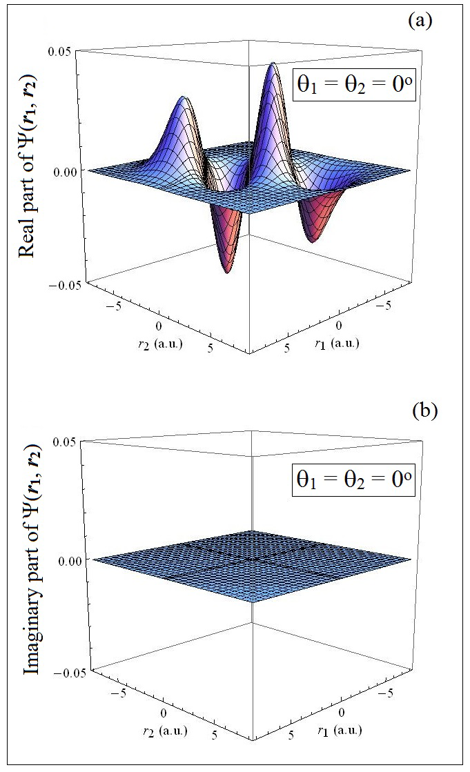
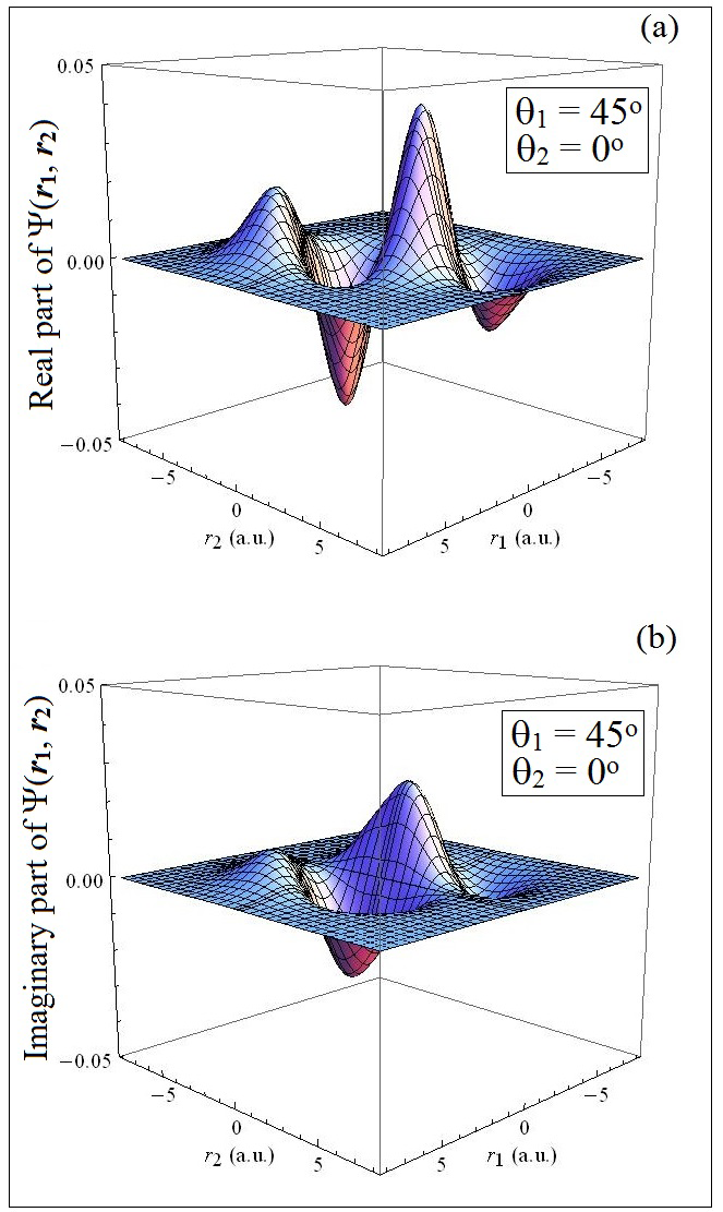
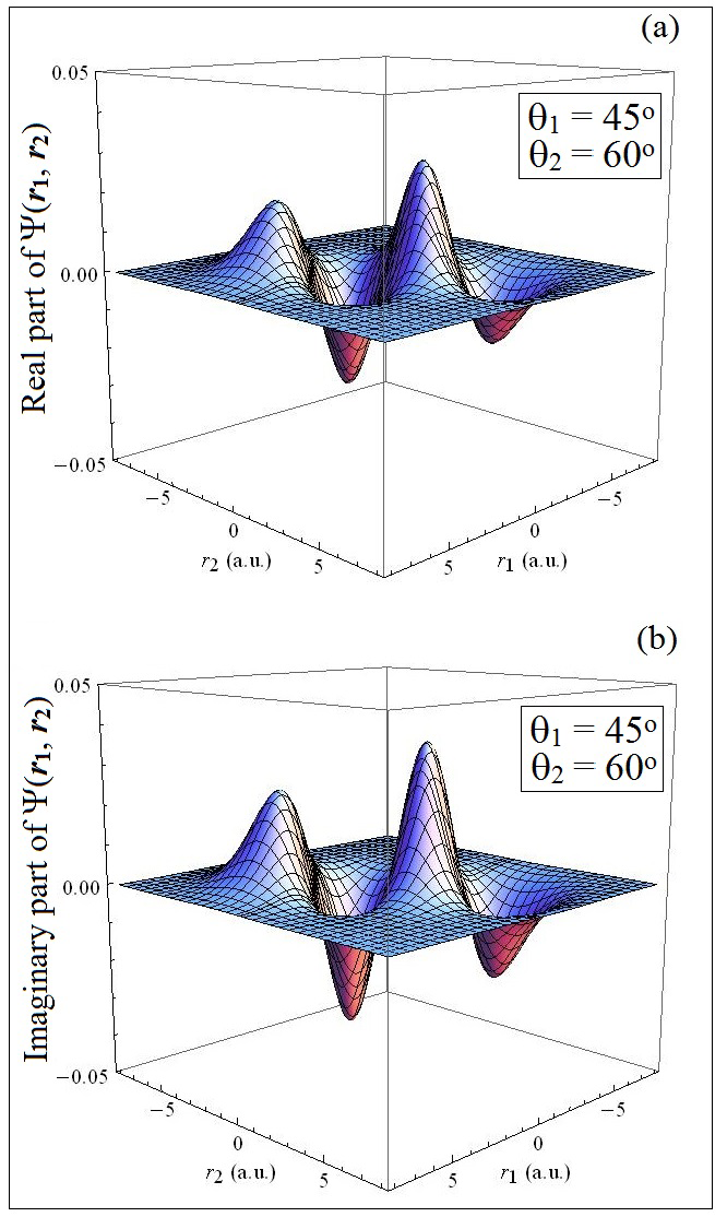
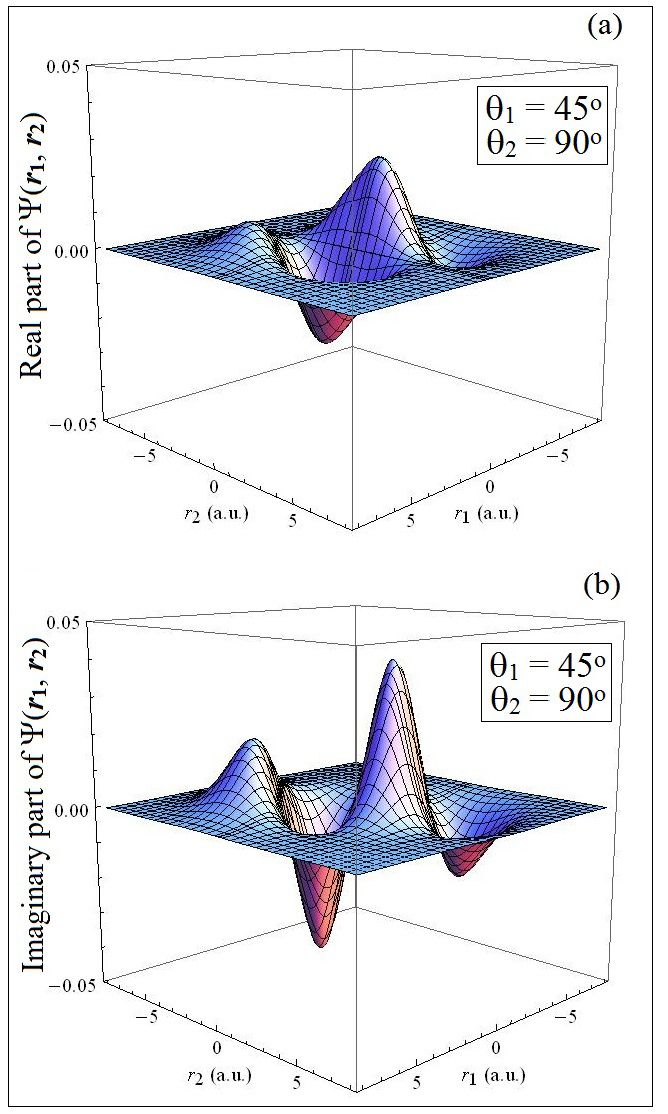
1. In Figs. 1 - 4 we plot the function $\Psi({\bf{r}}_{1}{\bf{r}}_{2})$ as a function of $r_{1}$ and $r_{2}$ for different $\theta_{1}$ and $\theta_{2}$. In each figure, panel (a) corresponds to the real part of $\Psi({\bf{r}}_{1}{\bf{r}}_{2})$, and panel (b) to its imaginary part. Observe that in Fig. 1 for $\theta_{1}=\theta_{2}=0^{\circ}$, the function $\Psi({\bf{r}}_{1}{\bf{r}}_{2})$ is real. As $\theta_{1}$ increases to $\theta_{1}=45^{\circ}$ in Fig. 2, the real part shrinks and the imaginary part becomes finite. For fixed $\theta_{1}=45^{\circ}$ and increasing $\theta_{2}=60^{\circ},90^{\circ}$ as in Figs. 3 and 4, respectively, the real part continues to diminish whilst the imaginary part increases in magnitude.

2. For an $N$ particle system, the coalescence condition 8 in $D$ dimensions of $2$ particles of masses $m_{1}$ and $m_{2}$, and charges $Z_{1}$ and $Z_{2}$, (with the spin index suppressed) is

$$\psi({\bf{r}}_{1},{\bf{r}}_{2},\ldots,{\bf{r}}_{N})=\psi({\bf{r}}_{2},{\bf{r}}_{2},{\bf{r}}_{3},\ldots,{\bf{r}}_{N})\bigg{(}1+\frac{2Z_{1}Z_{2}\mu_{12}}{D-1}u\bigg{)}$$

$$+{\bf{u}}\cdot{\bf{C}}({\bf{r}}_{2},{\bf{r}}_{3},\ldots,{\bf{r}}_{N}),$$ (8)

where $\mu_{12}=m_{1}m_{2}/m_{1}+m_{2}$ is the reduced mass, and ${\bf{C}}({\bf{r}}_{2},{\bf{r}}_{3},\ldots,{\bf{r}}_{N})$ is an undetermined vector. This is the integral form of the cusp coalescence condition. It is equally valid when the wave function vanishes at the point of coalescence, i.e. when $\psi({\bf{r}}_{2},{\bf{r}}_{2},{\bf{r}}_{3},\ldots,{\bf{r}}_{N})=0$, and is then referred to as the node coalescence condition. The wave function $\psi({\bf{x}}_{1}{\bf{x}}_{2})$ for the triplet state via its spatial component $\Psi({\bf{r}}_{1}{\bf{r}}_{2})$ satisfies the node electron-electron coalescence condition.

3. The function $\Psi({\bf{r}}_{1}{\bf{r}}_{2})$ exhibits the following nodes.

(a) There is a node at the origin. This is evident in Figs. 1 - 4 for both the cases of $\theta_{1}=\theta_{2}$ and $\theta_{1}\neq\theta_{2}$. This is because the probability of $2$ electrons of the same spin being at the same position in space at ${\bf{r}}_{1}={\bf{r}}_{2}=0$ is zero as a result of the Pauli exclusion principle. Observe also that the parity of the function $\Psi({\bf{r}}_{1}{\bf{r}}_{2})$ about the origin is odd.

(b) There is a node 19 at all points of electron-electron coalescence, again as a consequence of the Pauli exclusion principle. The function $\Psi({\bf{r}}_{1}{\bf{r}}_{2})$ has odd parity about all these points of coalescence.

(c) The real part of $\Psi({\bf{r}}_{1}{\bf{r}}_{2})$ has a node 19 when the projections of the vectors ${\bf{r}}_{1}$ and ${\bf{r}}_{2}$ on the x-axis are the same. The function $\Psi({\bf{r}}_{1}{\bf{r}}_{2})$ is then purely imaginary. The parity of the $\Psi({\bf{r}}_{1}{\bf{r}}_{2})$ is odd about the line ${\bf{r}}_{2}=(cos\theta_{1}/cos\theta_{2}){\bf{r}}_{1}$.

(d) The imaginary part of $\Psi({\bf{r}}_{1}{\bf{r}}_{2})$ has a node 19 when the projections of the vectors ${\bf{r}}_{1}$ and ${\bf{r}}_{2}$ on the y-axis are the same. The wave function is then real. The parity of $\Psi({\bf{r}}_{1}{\bf{r}}_{2})$ is odd about the line ${\bf{r}}_{2}=(sin\theta_{1}/sin\theta_{2}){\bf{r}}_{1}$ .

(e) There is a node of $\Psi({\bf{r}}_{1}{\bf{r}}_{2})$ as a result of it being a first excited state. These nodes are located where $\Psi({\bf{r}}_{1}{\bf{r}}_{2})$ is zero along the lines at non-zero values of $r_{1}$ and $r_{2}$ as shown in Figs. 1-4. There is no parity of $\Psi({\bf{r}}_{1}{\bf{r}}_{2})$ about this node.

III QUANTAL SOURCES

In this section we describe the various quantal sources for the fields that satisfy the ‘Quantal Newtonian’ first law. As the spin and spatial coordinates are separable, and the corresponding spin $\chi({\bf{\sigma}}_{1}{\bf{\sigma}}_{2})$ and spatial $\Psi({\bf{r}}_{1}{\bf{r}}_{2})$ components are separately normalized, the quantal sources are simply expectation values taken with respect to the spatial component. The analytical and semi-analytical expressions for the sources are given in Appendix A.

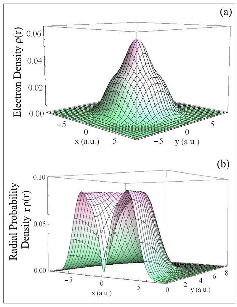
(i) Electron Density $\rho({\bf{r}})$

The electron density $\rho({\bf{r}})$ is the expectation value

$$\rho({\bf{r}})=\langle\Psi|\hat{\rho}({\bf{r}})|\Psi\rangle,$$ (9)

where the density operator $\hat{\rho}({\bf{r}})$ is

$$\hat{\rho}({\bf{r}})=\sum_{k}\delta({\bf{r}}_{k}-{\bf{r}}).$$ (10)

In Fig. 5a the electron density $\rho({\bf{r}})$ is plotted. It is spherically symmetric about the origin, and exhibits shell structure. As a consequence of the binding potential being harmonic, the density is finite at the origin and does not exhibit a cusp there. It is a local or static property in that its overall structure remains unchanged as the electron position is varied. In Fig. 5b, the radial probability density $r\rho({\bf{r}})$ is plotted, and again shell structure is clearly evident in the shoulder.

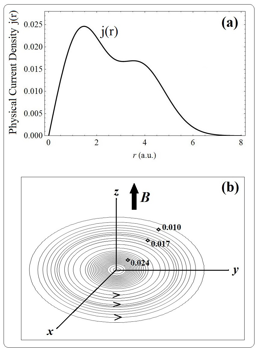
(ii) Physical Current Density ${\bf{j}}({\bf{r}})$

The physical current density ${\bf{j}}({\bf{r}})$, a local property, is the expectation value

$${\bf{j}}({\bf{r}})=\langle\Psi|\hat{\bf{j}}({\bf{r}})|\Psi\rangle,$$ (11)

where the current density operator $\hat{\bf{j}}({\bf{r}})$ is the sum of its paramagnetic $\hat{\bf{j}}_{p}({\bf{r}})$, diamagnetic $\hat{\bf{j}}_{d}({\bf{r}})$, and magnetization $\hat{\bf{j}}_{m}({\bf{r}})$ current density components:

$$\hat{\bf{j}}({\bf{r}})=\hat{\bf{j}}_{p}({\bf{r}})+\hat{\bf{j}}_{d}({\bf{r}})+\hat{\bf{j}}_{m}({\bf{r}}),$$ (12)

with

$$\hat{\bf{j}}_{p}({\bf{r}}) = \frac{1}{2}\sum_{k}\bigg{[}\hat{\bf{p}}_{k}\delta({\bf{r}}_{k}-{\bf{r}})+\delta({\bf{r}}_{k}-{\bf{r}})\hat{\bf{p}}_{k}\bigg{]},$$ (13)

$$\hat{\bf{j}}_{d}({\bf{r}}) = \hat{\rho}({\bf{r}}){\bf{A}}({\bf{r}}),$$ (14)

$$\hat{\bf{j}}_{m}({\bf{r}}) = -{\boldsymbol{\nabla}}\times\hat{\bf{m}}({\bf{r}})$$ (15)

and the magnetization density $\hat{\bf{m}}({\bf{r}})$ operator is

$$\hat{\bf{m}}({\bf{r}})=\sum_{k}{\bf{s}}_{k}\delta({\bf{r}}_{k}-{\bf{r}}).$$ (16)

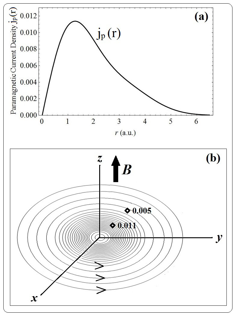
The paramagnetic current density ${\bf{j}}_{p}({\bf{r}})$ may also be defined via the quantal source of the single-particle density matrix $\gamma({\bf{rr}}^{\prime})$ as

$${\bf{j}}_{p}({\bf{r}})=\frac{1}{2}\bigg{[}{\boldsymbol{\nabla}}^{\prime}-{\boldsymbol{\nabla}}^{\prime\prime}\bigg{]}\gamma({\bf{r}}^{\prime}{\bf{r}}^{\prime\prime})\bigg{|}_{{\bf{r}}^{\prime}={\bf{r}}^{\prime\prime}=r},$$ (17)

where $\gamma({\bf{rr}}^{\prime})$ is defined below in subsection (iv). (The expression for $\hat{\bf{j}}_{p}({\bf{r}})$ for this triplet state given in Appendix A is derived independently through the definitions of Eqs. (13) and (17).)

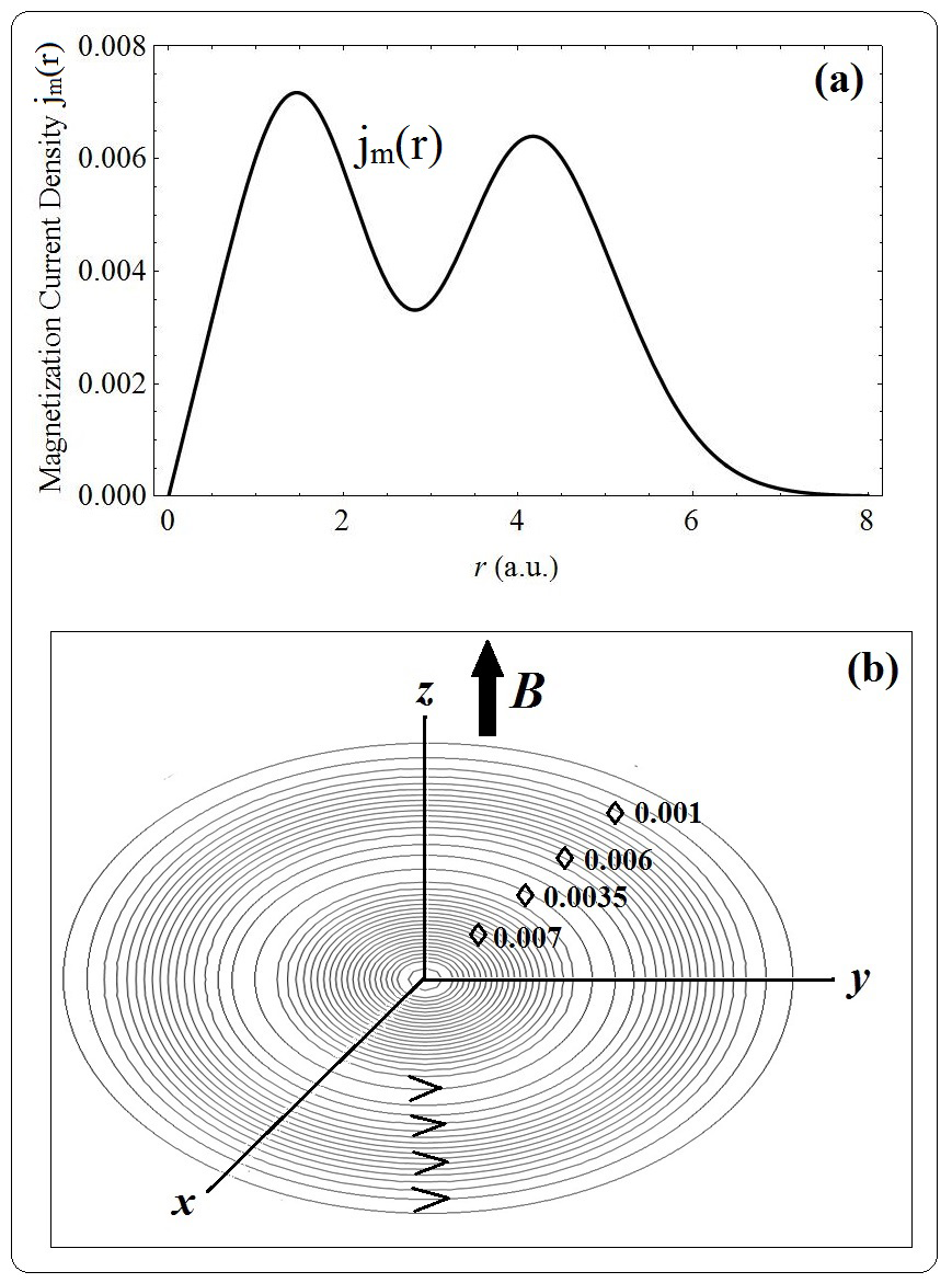
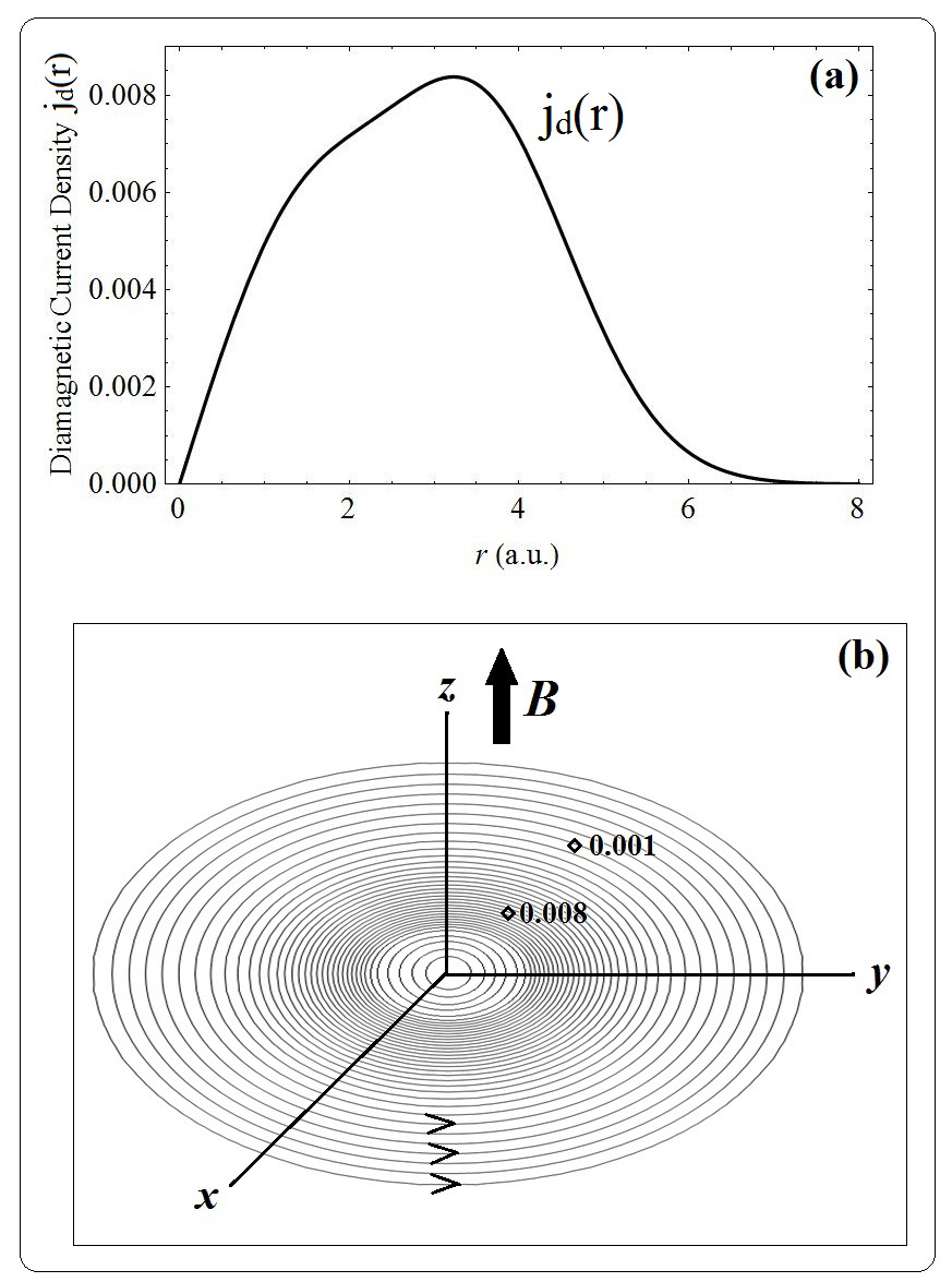
In Figs. 6 - 9 panels (a), the physical current density ${\bf{j}}({\bf{r}})$, and its paramagnetic ${\bf{j}}_{p}({\bf{r}})$, diamagnetic ${\bf{j}}_{d}({\bf{r}})$, and magnetization ${\bf{j}}_{m}({\bf{r}})$ components, respectively, are plotted. The diamagnetic component ${\bf{j}}_{d}({\bf{r}})$ which is the only component that depends explicitly on the magnetic field is plotted for a value of the Larmor frequency of $\omega_{L}=0.1$. Hence, the plot of the total current density ${\bf{j}}({\bf{r}})$ is for $\omega_{L}=0.1$. Each density component is a function solely of the radial component $r$, but points in the $\hat{\bf{i}}_{\theta}$ direction. Hence, the divergence of each component vanishes, and therefore ${\boldsymbol{\nabla}}\cdot{\bf{j}}({\bf{r}})=0$.

Observe that shell structure is clearly evident in the plot of the current density ${\bf{j}}({\bf{r}})$ (see Fig. 6a). This structure is also evident in the individual components (see Figs. 7a - 9a), although their individual structures are different. For the choice of $\omega_{L}=0.1$, the magnitude of the paramagnetic ${\bf{j}}_{p}({\bf{r}})$, diamagnetic ${\bf{j}}_{d}({\bf{r}})$, and magnetization ${\bf{j}}_{m}({\bf{r}})$ components is essentially the same. (Depending on the value of $\omega_{L}$, the diamagnetic component ${\bf{j}}_{d}({\bf{r}})$ and thus ${\bf{j}}({\bf{r}})$ can be made larger or smaller.)

In Figs. 6 - 9, panels (b), the flow line contours of each current density component are plotted. These contour lines are closest in the regions of greater density. Observe the difference in the contours for each density component. The circulation direction of the component ${\bf{j}}_{p}({\bf{r}})$ depends explicitly on the choice of angular momentum quantum number $m$. This is also the case for ${\bf{j}}_{m}({\bf{r}})$ whose dependency on $m$ is via the electronic density $\rho_{\uparrow\uparrow}$ (corresponding to m = 1) or $\rho_{\downarrow\downarrow}$ (corresponding to $m=-1$). The circulation direction of these two current densities ${\bf{j}}_{p}({\bf{r}})$ and ${\bf{j}}_{m}({\bf{r}})$ is always the same, but the direction depends upon whether $m=1$ or $m=-1$. On the other hand, the diamagnetic current density ${\bf{j}}_{d}({\bf{r}})$ does not depend on $m$. Thus, its circulation can be either in the same or opposite direction to that of ${\bf{j}}_{p}({\bf{r}})$ depending on the value of $m$. For our choice of $m=1$, the circulation direction for ${\bf{j}}_{p}({\bf{r}})$, ${\bf{j}}_{d}({\bf{r}})$, and ${\bf{j}}_{m}({\bf{r}})$ are all the same (counterclockwise). (The fact that the circulation directions of ${\bf{j}}_{p}({\bf{r}})$ and ${\bf{j}}_{d}({\bf{r}})$ are the same, for the chosen value of $m$, has been confirmed by an independent derivation related to the contribution of the Lorentz ${\boldsymbol{\cal{L}}}({\bf{r}})$ and internal magnetic ${\boldsymbol{\cal{I}}}_{m}({\bf{r}})$ fields to the total energy.)

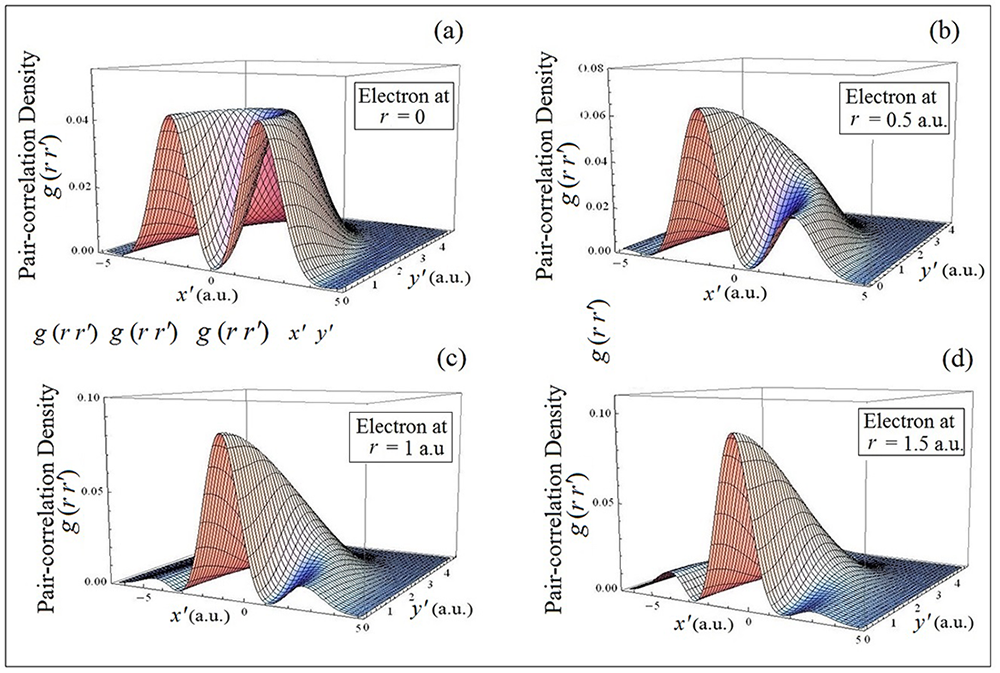
(iii) Pair-correlation Density $g({\bf{rr}}^{\prime})$ and the Fermi-Coulomb hole $\rho_{xc}({\bf{rr}}^{\prime})$

The pair-correlation density $g({\bf{rr}}^{\prime})$ is defined as the ratio of the pair-correlation function $P({\bf{rr}}^{\prime})$ to the density $\rho({\bf{r}})$:

$$g({\bf{rr}}^{\prime})=P({\bf{rr}}^{\prime})/\rho({\bf{r}}),$$ (18)

where $P({\bf{rr}}^{\prime})$ is the expectation value

$$P({\bf{rr}}^{\prime})=\langle\Psi|\hat{P}({\bf{rr}}^{\prime})|\Psi\rangle,$$ (19)

with the pair operator defined as

$$\hat{P}({\bf{rr}}^{\prime})=\sideset{}{{}^{\prime}}{\sum}_{k,\ell}\delta({\bf{r}}_{k}-{\bf{r}})\delta({\bf{r}}_{\ell}-{\bf{r}}^{\prime}).$$ (20)

The pair-correlation density $g({\bf{rr}}^{\prime})$ may also be written in terms of its local and nonlocal components as

$$g({\bf{rr}}^{\prime})=\rho({\bf{r}}^{\prime})+\rho_{xc}({\bf{rr}}^{\prime}),$$ (21)

where $\rho_{xc}({\bf{rr}}^{\prime})$ is the Fermi-Coulomb hole charge.

The pair-correlation density $g({\bf{rr}}^{\prime})$ and Fermi-Coulomb hole $\rho_{xc}({\bf{rr}}^{\prime})$ are nonlocal quantal sources in that their structure changes as a function of the electron position. This is demonstrated in Fig. 10 where $g({\bf{rr}}^{\prime})$ is plotted for the following different electron positions: (a) the center of the quantum dot at $r=0$; (b) at $r=0.5~{}a.u.$; (c) at $r=1.0~{}a.u.$;(d) at $r=1.5~{}a.u.$ Observe that in each figure, the pair-correlation density vanishes at the electron position. This is a consequence of the node coalescence condition satisfied by the wave function. 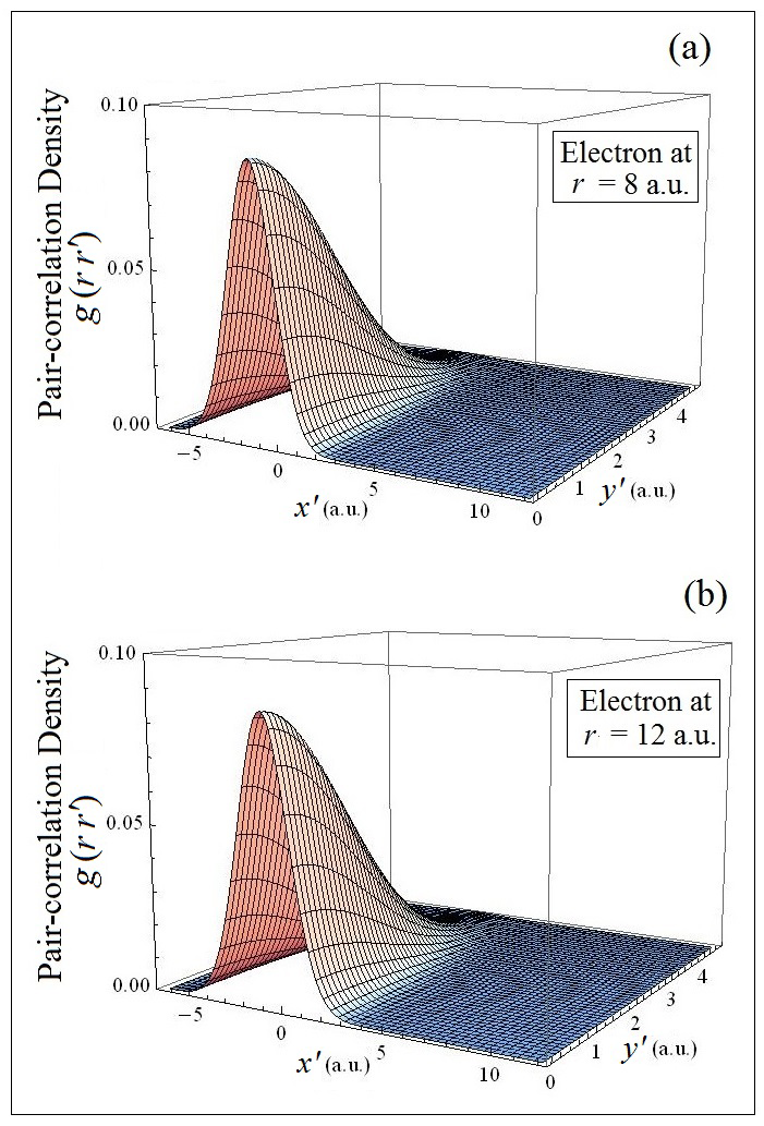Also note that except for the electron position at the center of the quantum dot, $g({\bf{rr}}^{\prime})$ is not spherically symmetric about the electron position. In Fig. 11, the $g({\bf{rr}}^{\prime})$ is plotted for asymptotic positions of the electron: (a) at $r=8.0~{}a.u.$; (b) at $r=12.0~{}a.u.$ For these asymptotic positions, observe that the figures are very similar. This is a reflection of the fact that for such asymptotic positions of the electron, the nonlocal charge is becoming essentially static. Since the total charge of the pair-correlation density $g({\bf{rr}}^{\prime})$ is $1$ (obtained from $N-1$), the asymptotic structure of the electron-interaction field ${\boldsymbol{\cal{E}}}_{\mathrm{ee}}({\bf{r}})$ derived from it via Coulomb’s law is analytically known (see Sect. IV). Since for an electron at the center of the quantum dot, the density $g({\bf{rr}}^{\prime})$ is spherically symmetric about this position(Fig. 10a), the field vanishes there.

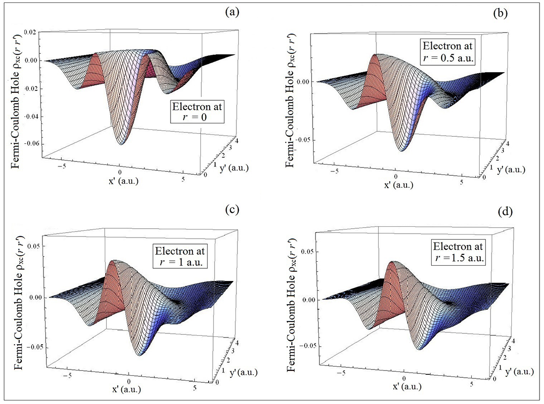
The nonlocal structure of the Fermi-Coulomb hole $\rho_{xc}({\bf{rr}}^{\prime})$ (see Fig. 12) can be obtained from Eq. (21). The hole represents the reduction in density at ${\bf{r}}^{\prime}$ for an electron at ${\bf{r}}$ due to the Pauli exclusion principle and Coulomb repulsion. Although this structure differs significantly from that of $g({\bf{rr}}^{\prime})$, its properties are similar. Thus, at the electron position, the hole is finite and continuous and has the lowest value. (There is no cusp at this point as is the case for a singlet excited state.) For an electron position at the center of the quantum dot, the hole is spherically symmetric about it, and thus the Pauli-Coulomb field ${\boldsymbol{\cal{E}}}_{\mathrm{xc}}({\bf{r}})$ vanishes at the origin. The hole is not spherically symmetric about the other electron positions. As the hole becomes an essentially static charge for asymptotic positions of the electron, and since the total hole charge is $-1$, the asymptotic structure of ${\boldsymbol{\cal{E}}}_{\mathrm{xc}}({\bf{r}})$ is also analytically known (see Sect. IV.).

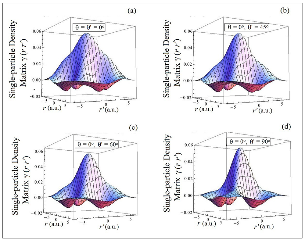
(iv) Single-Particle Density Matrix $\gamma({\bf{rr}}^{\prime})$

The single-particle density matrix $\gamma({\bf{rr}}^{\prime})$, a nonlocal quantal source, is defined as the expectation value

$$\gamma({\bf{rr}}^{\prime})=\langle\Psi|\hat{\gamma}({\bf{rr}}^{\prime})|\Psi\rangle,$$ (22)

where the complex single-particle density matrix operator 20 ; 21 is

$$\hat{\gamma}({\bf{rr}}^{\prime})=\hat{A}+i\hat{B},$$ (23)

$$\hat{A}=\frac{1}{2}\sum_{k}\big{[}\delta({\bf{r}}_{k}-{\bf{r}})T_{k}({\bf{a}})+\delta({\bf{r}}_{k}-{\bf{r}}^{\prime})T_{k}(-{\bf{a}})\big{]},$$ (24)

$$\hat{B}=\frac{i}{2}\sum_{k}\big{[}\delta({\bf{r}}_{k}-{\bf{r}})T_{k}({\bf{a}})-\delta({\bf{r}}_{k}-{\bf{r}}^{\prime})T_{k}(-{\bf{a}})\big{]},$$ (25)

with $T_{k}({\bf{a}})$ a translation operator such that $T_{k}({\bf{a}})\psi(\ldots{\bf{r}}_{k},\ldots)=\psi(\ldots{\bf{r}}_{k}+{\bf{a}},\ldots)$ and ${\bf{a}}={\bf{r}}^{\prime}-{\bf{r}}$. The operators $\hat{A}$ and $\hat{B}$ are Hermitian. The single-particle density matrix is the quantal source for all kinetic related properties 22 such as the kinetic energy tensor, the kinetic energy density, the kinetic field, the kinetic energy, and as noted above, the paramagnetic current density.

In the panels of Fig. 13, the $\gamma({\bf{rr}}^{\prime})$ for the triplet state is plotted as the positions ${\bf{r}}$ and ${\bf{r}}^{\prime}$ change for (a) $\theta=\theta^{\prime}=0^{\circ}$; (b) $\theta=0^{\circ}$, $\theta^{\prime}=45^{\circ}$; (c) $\theta=0^{\circ}$, $\theta^{\prime}=60^{\circ}$; (d) $\theta=0^{\circ}$, $\theta^{\prime}=90^{\circ}$. The nonlocal nature of $\gamma({\bf{rr}}^{\prime})$ is clearly evident as is shell structure. Observe the change in the shoulder of $\gamma({\bf{rr}}^{\prime})$ as $\theta^{\prime}$ changes from $0^{\circ}$ to $90^{\circ}$. Also note that the $\gamma({\bf{rr}}^{\prime})$ exhibits nodes as a consequence of the node in the wave function for this excited state (point #3e of Sect. II). Although the wave function exhibits a node at the origin (point # 3a), the $\gamma({\bf{rr}}^{\prime})$ is finite there. For the cross sections for which ${\bf{r}}={\bf{r}}^{\prime}$, one obtains the density of Fig.5 since $\gamma({\bf{rr}})=\rho({\bf{r}})$.

Table 1: Properties of the Triplet $2^{3}S$ state of the quantum dot in a magnetic field. The values are in effective atomic units $(a.u.)^{\star}$

Property	Value
$T$	0.615577
$E_{H}$	0.755497
$E_{xc}$	-0.501339
$E_{ee}$	0.254158
$E_{es}+E_{mag}$	0.742657
$E$	1.612391
$IP=E^{N-1}-E^{N}$	-1.343659
$\langle{\bf{r}}^{2}\rangle$	20.567403
$\langle r\rangle$	5.823553
$\langle 1/r\rangle$	1.041717
$\langle\delta({\bf{r}})\rangle$	0.0555377

IV ‘Forces’, Fields, and Energies

The ‘forces’ and fields derived from the quantal sources are described next. The contributions of the individual fields to the total energy $E$ are given in Table I. Various analytical and semi-analytical expressions for the fields and components of the energy are given in Appendix A.

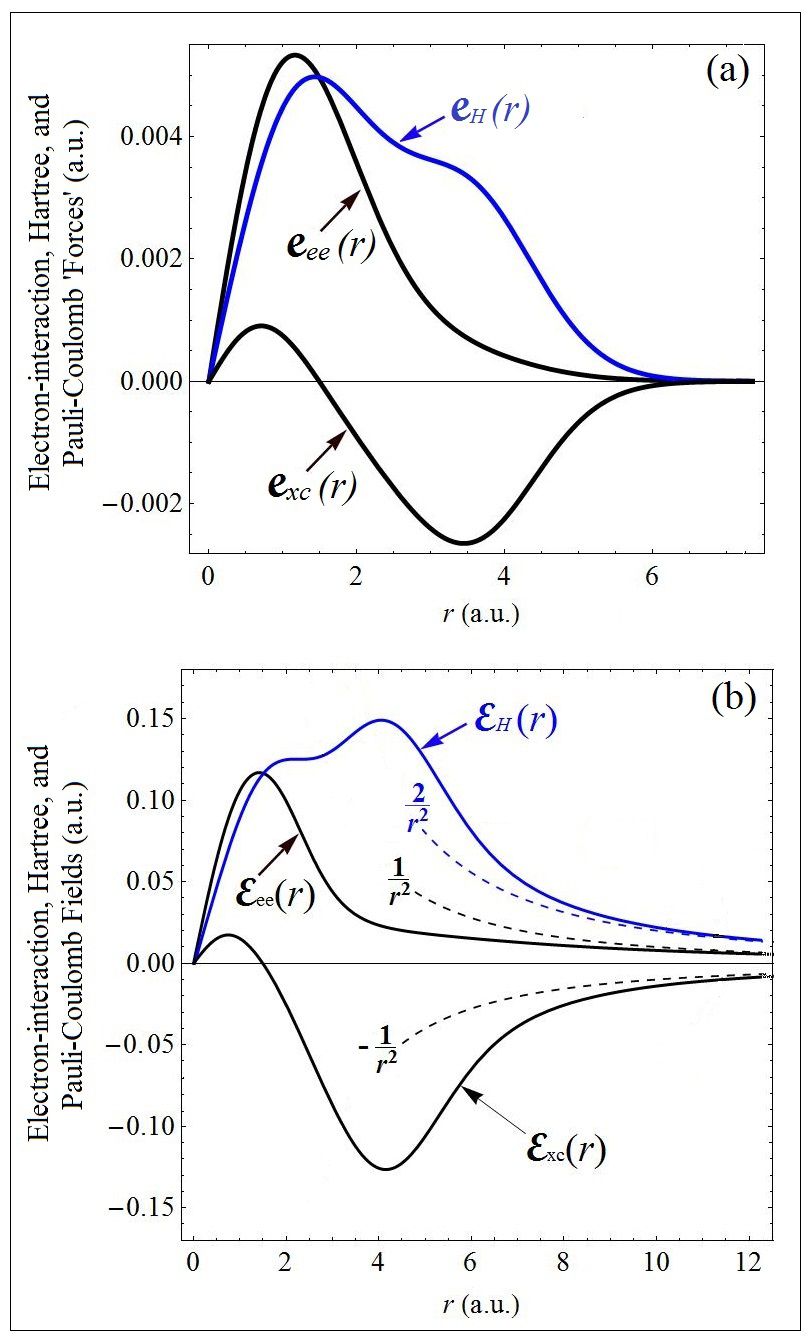
(i) Electron-interaction

The electron-interaction field ${\boldsymbol{\cal{E}}}_{\mathrm{ee}}({\bf{r}})$ is obtained from its quantal source, the pair-correlation density $g({\bf{rr}}^{\prime})$, via Coulomb’s law, and may be written (see Eq. (21)) in terms of its Hartree ${\boldsymbol{\cal{E}}}_{\mathrm{H}}({\bf{r}})$ and Pauli-Coulomb ${\boldsymbol{\cal{E}}}_{\mathrm{xc}}({\bf{r}})$ components:

$${\boldsymbol{\cal{E}}}_{\mathrm{ee}}({\bf{r}}) = \int\frac{g({\bf{rr}}^{\prime})({\bf{r}}-{\bf{r}}^{\prime})}{|{\bf{r}}-{\bf{r}}^{\prime}|^{3}}d{\bf{r}}^{\prime}$$ (26)

$$= {\boldsymbol{\cal{E}}}_{\mathrm{H}}({\bf{r}})+{\boldsymbol{\cal{E}}}_{\mathrm{xc}}({\bf{r}}),$$ (27)

where

$${\boldsymbol{\cal{E}}}_{\mathrm{H}}({\bf{r}})=\int\frac{\rho({\bf{r}}^{\prime})({\bf{r}}-{\bf{r}}^{\prime})}{|{\bf{r}}-{\bf{r}}^{\prime}|^{3}}d{\bf{r}}^{\prime}~{}~{};~{}~{}{\boldsymbol{\cal{E}}}_{\mathrm{xc}}({\bf{r}})=\int\frac{\rho_{\mathrm{xc}}({\bf{rr}}^{\prime})({\bf{r}}-{\bf{r}}^{\prime})}{|{\bf{r}}-{\bf{r}}^{\prime}|^{3}}d{\bf{r}}^{\prime}.$$ (28)

The fields may also be expressed in terms of their corresponding ‘forces’ ${\bf{e}}_{\mathrm{ee}}({\bf{r}})$, ${\bf{e}}_{\mathrm{H}}({\bf{r}})$, and ${\bf{e}}_{\mathrm{xc}}({\bf{r}})$:

$${\boldsymbol{\cal{E}}}_{\mathrm{ee}}({\bf{r}})={\bf{e}}_{\mathrm{ee}}({\bf{r}})/\rho({\bf{r}})~{};~{}{\boldsymbol{\cal{E}}}_{\mathrm{H}}({\bf{r}})={\bf{e}}_{\mathrm{H}}({\bf{r}})/\rho({\bf{r}})~{};~{}{\boldsymbol{\cal{E}}}_{\mathrm{xc}}({\bf{r}})={\bf{e}}_{\mathrm{xc}}({\bf{r}})/\rho({\bf{r}}).$$ (29)

In Fig. 14(a) and (b) we plot the various ‘forces’ and fields, respectively. Shell structure is evident in the plots of both the ‘forces’ and fields. (For the ‘force’ ${\bf{e}}_{\mathrm{ee}}({\bf{r}})$ and field ${\boldsymbol{\cal{E}}}_{\mathrm{ee}}({\bf{r}})$, the second shell becomes evident on an expanded scale.) As the quantal sources $g({\bf{rr}}^{\prime})$, $\rho({\bf{r}})$, $\rho_{\mathrm{xc}}({\bf{rr}}^{\prime})$ are all cylindrically symmetric for an electron position at the origin (see Figs. 5a, 10a, 12a), all the corresponding fields vanish there. Since for asymptotic positions of the electron in the classically forbidden region, the nonlocal sources $g({\bf{rr}}^{\prime})$ and $\rho_{\mathrm{xc}}({\bf{rr}}^{\prime})$ become essentially static charge distributions (see Fig. 11), and the density $\rho({\bf{r}})$ is a static charge, the asymptotic structure of the fields as $r\rightarrow\infty$ is known exactly: ${\boldsymbol{\cal{E}}}_{\mathrm{ee}}({\bf{r}})\sim 1/r^{2}$, ${\boldsymbol{\cal{E}}}_{\mathrm{H}}({\bf{r}})\sim 2/r^{2}$, ${\boldsymbol{\cal{E}}}_{\mathrm{xc}}({\bf{r}})\sim-1/r^{2}$. That the decay of these fields is such is clearly evident in Fig. 14(b). Asymptotically, the ‘forces’(see Fig. 14(a)) all vanish as their decay is faster than that of the density.

The electron-interaction $E_{\mathrm{ee}}$, Hartree $E_{\mathrm{H}}$, and Pauli-Coulomb $E_{\mathrm{xc}}$ energies are then obtained in integral virial form from the respective fields as (see Table I)

$$E_{\mathrm{ee}} = \int\rho({\bf{r}}){\bf{r}}\cdot{\boldsymbol{\cal{E}}}_{\mathrm{ee}}({\bf{r}})d{\bf{r}},$$ (30)

$$E_{\mathrm{H}} = \int\rho({\bf{r}}){\bf{r}}\cdot{\boldsymbol{\cal{E}}}_{\mathrm{H}}({\bf{r}})d{\bf{r}},$$ (31)

$$E_{\mathrm{xc}} = \int\rho({\bf{r}}){\bf{r}}\cdot{\boldsymbol{\cal{E}}}_{\mathrm{xc}}({\bf{r}})d{\bf{r}}.$$ (32)

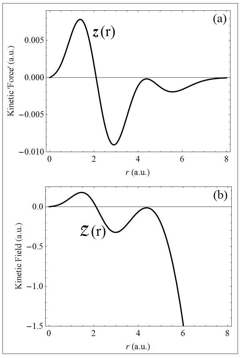
(ii) Kinetic

The quantal source for the kinetic ‘force’ ${\bf{z}}({\bf{r}})$, field ${\boldsymbol{\cal{Z}}}({\bf{r}})$, and energy $T$ is the single-particle density matrix $\gamma({\bf{rr}}^{\prime})$. The field is defined in terms of the ‘force’ as

$${\boldsymbol{\cal{Z}}}({\bf{r}})={\bf{z}}({\bf{r}})/\rho({\bf{r}}),$$ (33)

where in Cartesian coordinates

$$z_{\alpha}({\bf{r}})=2\sum_{\beta}\nabla_{\beta}t_{\alpha\beta}({\bf{r}};\gamma),$$ (34)

and where the second-rank kinetic energy tensor

$$t_{\alpha\beta}({\bf{r}};\gamma)=\frac{1}{4}\bigg{[}\frac{\partial^{2}}{\partial r^{\prime}_{\alpha}\partial r^{\prime\prime}_{\beta}}+\frac{\partial^{2}}{\partial r^{\prime}_{\beta}\partial r^{\prime\prime}_{\alpha}}\bigg{]}\gamma({\bf{r}}^{\prime}{\bf{r}}^{\prime\prime})\bigg{|}_{{\bf{r}}^{\prime}={\bf{r}}^{\prime\prime}=r}.$$ (35)

The kinetic energy in terms of the field ${\boldsymbol{\cal{Z}}}({\bf{r}})$ is

$$T=-\frac{1}{2}\int\rho({\bf{r}}){\bf{r}}\cdot{\boldsymbol{\cal{Z}}}({\bf{r}})d{\bf{r}}.$$ (36)

The kinetic ‘force’ $z({\bf{r}})$ and field ${\boldsymbol{\cal{Z}}}({\bf{r}})$ are plotted in Fig. 15 (a) and (b), respectively. Once again, shell structure is evident. Whilst the ‘force’ $z({\bf{r}})$ decays and vanishes asymptotically, the field ${\boldsymbol{\cal{Z}}}({\bf{r}})$ is singular in this region. Both vanish at the origin. See Table I for the value of $T$. (For the derivation of the tensor $t_{\alpha\beta}({\bf{r}};\gamma)$ and the kinetic ‘force’ ${\bf{z}}({\bf{r}})$, see Appendix B.)

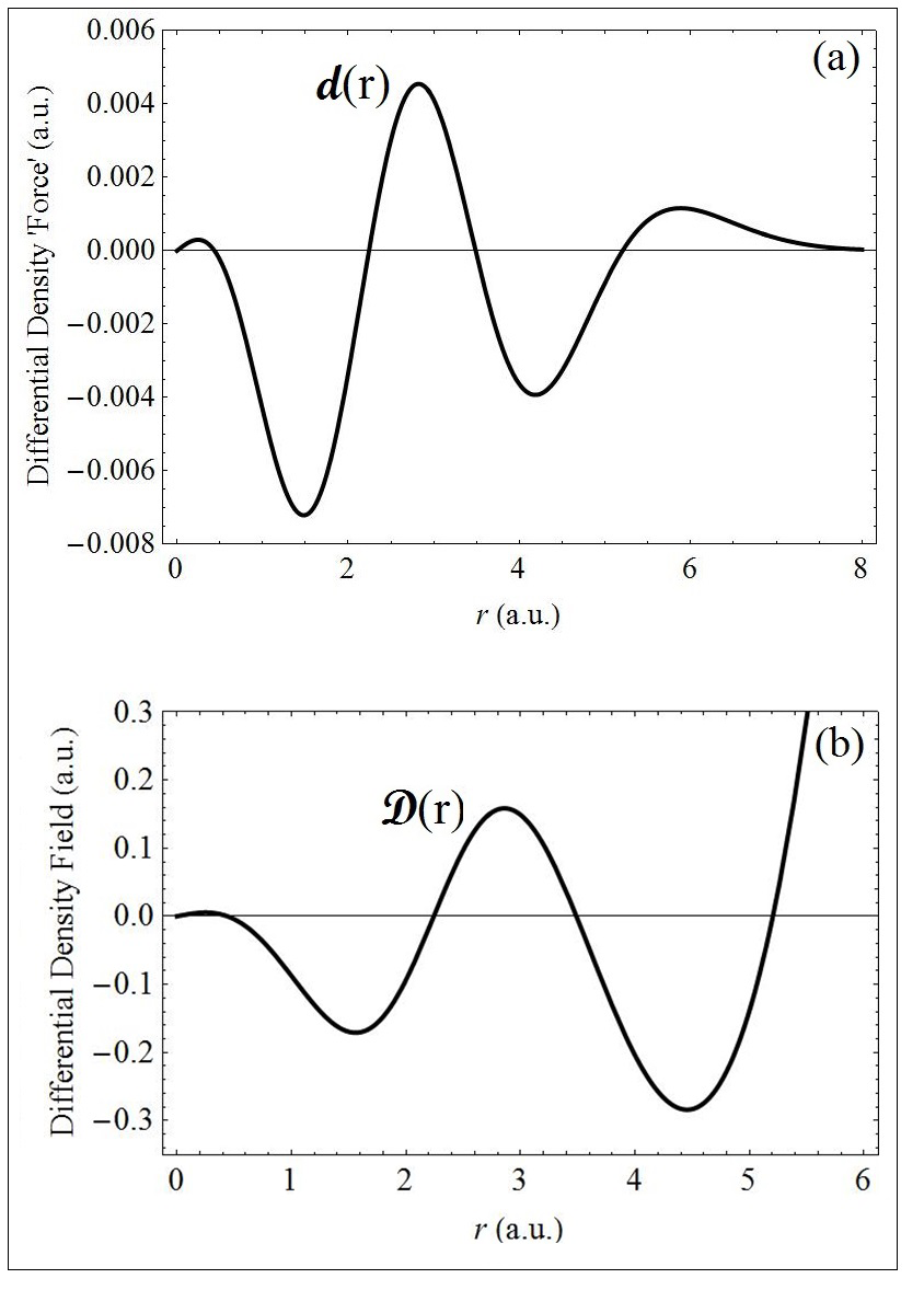
(iii) Differential Density

The quantal source for the differential density ‘force’ ${\bf{d}}({\bf{r}})$ and field ${\boldsymbol{\cal{D}}}({\bf{r}})$ is the density $\rho({\bf{r}})$. The field ${\boldsymbol{\cal{D}}}({\bf{r}})$ is defined as

$${\boldsymbol{\cal{D}}}({\bf{r}})={\bf{d}}({\bf{r}})/\rho({\bf{r}}),$$ (37)

where

$${\bf{d}}({\bf{r}})=-\frac{1}{4}{\boldsymbol{\nabla}}\nabla^{2}\rho({\bf{r}}).$$ (38)

The ‘force’ ${\bf{d}}({\bf{r}})$ and field ${\boldsymbol{\cal{D}}}({\bf{r}})$ are plotted in Fig. 16 (a) and (b), respectively. Their structure is similar to the kinetic case. The ‘force’ ${\bf{d}}({\bf{r}})$ and field ${\boldsymbol{\cal{D}}}({\bf{r}})$ exhibit shell structure, they both vanish at the origin, the ‘force’ decays asymptotically, whereas the field is singular in that region. There is no direct contribution of this field to the energy, however, its quantal source $\rho({\bf{r}})$ is the source for the Hartree field ${\boldsymbol{\cal{E}}}_{\mathrm{H}}({\bf{r}})$, and contributes to the energy through every contribution of the other energy components such as ${\boldsymbol{\cal{E}}}_{\mathrm{ee}}({\bf{r}})$, $T$, etc. (see Eqs. (30), (36), (47), and (48)).

(iv) Lorentz, Internal Magnetic, and External Electrostatic

The quantal source for the Lorentz and internal magnetic ‘forces’ $({\boldsymbol{\ell}}({\bf{r}}),{\bf{i}}_{m}({\bf{r}}))$ and fields $({\boldsymbol{\cal{L}}}({\bf{r}}),{\boldsymbol{\cal{I}}}_{m}({\bf{r}}))$ is the physical current density ${\bf{j}}({\bf{r}})$. The Lorentz field ${\boldsymbol{\cal{L}}}({\bf{r}})$ is defined as

$${\boldsymbol{\cal{L}}}({\bf{r}})={\boldsymbol{\ell}}({\bf{r}})/\rho({\bf{r}}),$$ (39)

where

$${\boldsymbol{\ell}}({\bf{r}})={\bf{j}}({\bf{r}})\times{\boldsymbol{\cal{B}}}({\bf{r}}),$$ (40)

or in Cartesian coordinates

$$\ell_{\alpha}({\bf{r}})=\sum_{\beta}\big{[}j_{\beta}({\bf{r}})\nabla_{\alpha}A_{\beta}({\bf{r}})-j_{\beta}({\bf{r}})\nabla_{\beta}A_{\alpha}({\bf{r}})\big{]}.$$ (41)

The internal magnetic field ${\boldsymbol{\cal{I}}}_{m}({\bf{r}})$ is defined as

$${\boldsymbol{\cal{I}}}_{m}({\bf{r}})={\bf{i}}_{m}({\bf{r}})/\rho({\bf{r}}),$$ (42)

where in Cartesian coordinates

$$i_{m,\alpha}({\bf{r}})=\sum_{\beta}\nabla_{\beta}I_{\alpha\beta}({\bf{r}}),$$ (43)

and where the second-rank tensor

$$I_{\alpha\beta}({\bf{r}})=\big{[}j_{\alpha}({\bf{r}})A_{\beta}({\bf{r}})+j_{\beta}({\bf{r}})A_{\alpha}({\bf{r}})\big{]}-\rho({\bf{r}})A_{\alpha}({\bf{r}})A_{\beta}({\bf{r}}).$$ (44)

We next define the field ${\boldsymbol{\cal{M}}}({\bf{r}})$ as

$${\boldsymbol{\cal{M}}}({\bf{r}})=-\big{[}{\boldsymbol{\cal{L}}}({\bf{r}})+{\boldsymbol{\cal{I}}}_{m}({\bf{r}})\big{]}.$$ (45)

Then, if ${\boldsymbol{\nabla}}\times{\boldsymbol{\cal{M}}}({\bf{r}})=0$, as is the case in the present application, one can define a path-independent scalar magnetic potential $v_{m}({\bf{r}})$ such that

$${\boldsymbol{\cal{M}}}({\bf{r}})=-{\boldsymbol{\nabla}}v_{m}({\bf{r}})/e.$$ (46)

Hence, the contribution to the energy $E_{\mathrm{mag}}$ of the sum of the Lorentz and internal magnetic fields ${\boldsymbol{\cal{M}}}({\bf{r}})$ is

$$E_{\mathrm{mag}}=\int\rho({\bf{r}})v_{m}({\bf{r}})d{\bf{r}}.$$ (47)

In a similar manner, as the external electrostatic field ${\boldsymbol{\cal{E}}}({\bf{r}})=-{\boldsymbol{\nabla}}v({\bf{r}})/e$ is curl free, the contribution to the energy $E_{\mathrm{es}}$ due to this field is

$$E_{\mathrm{es}}=\int\rho({\bf{r}})v({\bf{r}})d{\bf{r}}.$$ (48)

(The expression for $E_{\mathrm{es}}$ can also be obtained directly from the Hamiltonian of Eq. (2) as the expectation value of the operator $\hat{V}$.)

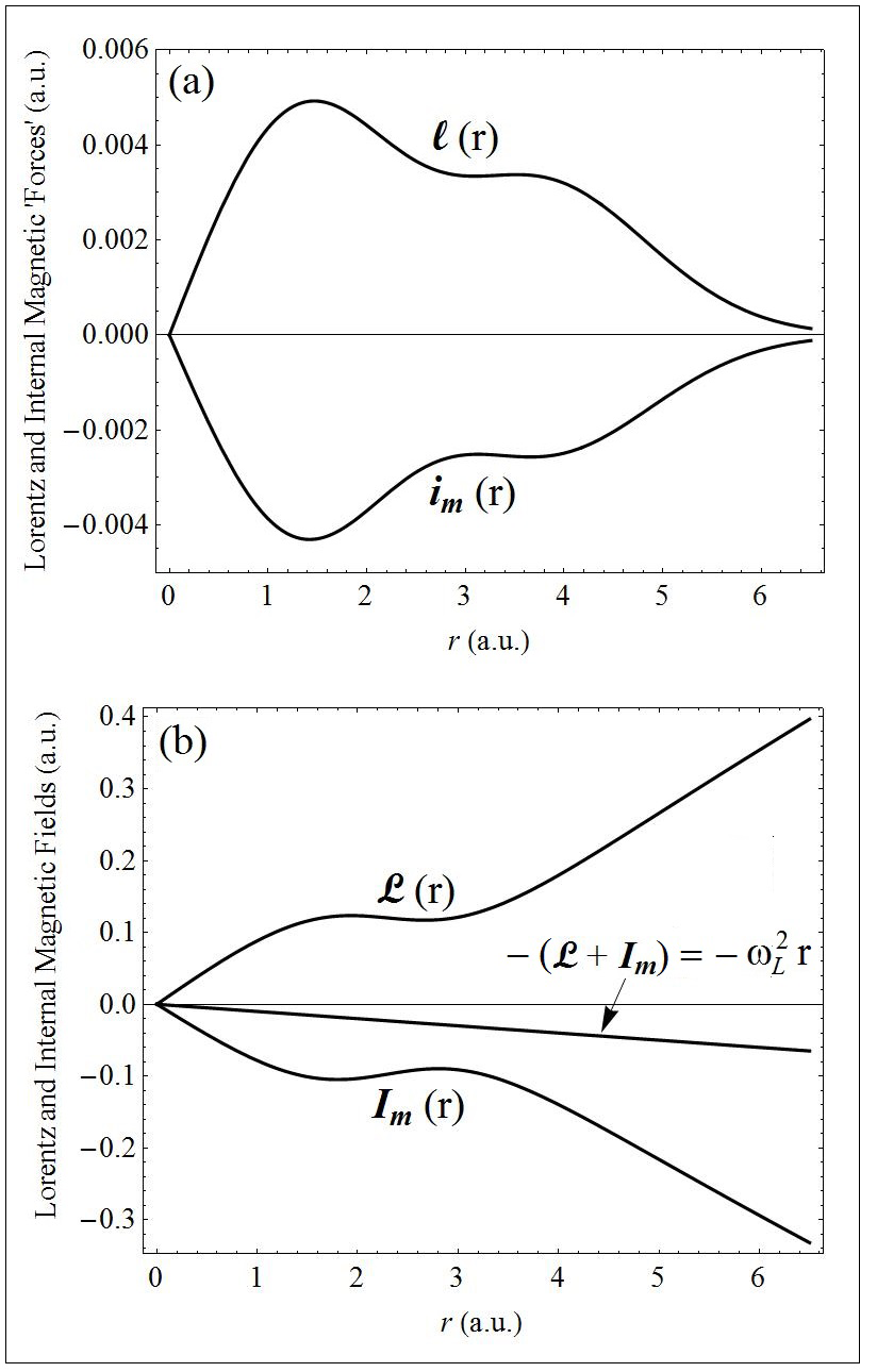
Both the Lorentz and internal magnetic ‘forces’ $({\boldsymbol{\ell}}({\bf{r}}),{\bf{i}}_{m}({\bf{r}}))$ and fields (${\boldsymbol{\cal{L}}}({\bf{r}}),{\boldsymbol{\cal{I}}}_{m}({\bf{r}}))$ depend on the strength of the magnetic field. In Fig. 17, these ‘forces’ and fields are plotted for a value of the Larmor frequency of $\omega_{L}=0.1$. Again, observe that these properties exhibit shell structure. The ‘forces’ Fig. 17 (a) vanish at the origin and asymptotically in the classically forbidden region. The fields Fig. 17 (b) vanish at the origin, but are singular asymptotically. For this triplet state of the quantum dot, it turns out that

$${\boldsymbol{\cal{M}}}({\bf{r}})=-\omega^{2}_{L}r\hat{\bf{i}}_{r},$$ (49)

and this linear function is also plotted in Fig. 17 (b). It follows from Eqs. (46) and (49) that (in $a.u.)^{\star}$

$$v_{m}({\bf{r}})=\frac{1}{2}\omega^{2}_{L}r^{2}.$$ (50)

Thus, the sum of the electrostatic $E_{\mathrm{es}}$ and magnetostatic $E_{\mathrm{mag}}$ energies is

$$E_{\mathrm{es}}+E_{\mathrm{mag}} = \int\rho(r)\bigg{\{}\frac{1}{2}\bigg{[}\omega^{2}_{0}+\omega^{2}_{L}\bigg{]}\bigg{\}}d{\bf{r}}$$ (51)

$$= \int\rho(r)\bigg{[}\frac{1}{2}k_{\mathrm{eff}}r^{2}\bigg{]}d{\bf{r}},$$ (52)

where $k_{\mathrm{eff}}=\omega_{0}^{2}+\omega_{L}^{2}=0.072217$ (see Sect. II). The value of this sum of energies is given in Table I.

The total energy of this triplet $2^{3}S$ state can then be written as

$$E=T+E_{H}+E_{\mathrm{xc}}+E_{\mathrm{es}}+E_{\mathrm{mag}}=1.612391~{}(a.u.)^{\star}.$$ (53)

(This value is consistent with the eigenvalue for the triplet state obtained by solution of the Schrödinger-Pauli equation Eq. (1).) The ionization potential defined as $IP=E^{N=1}-E^{N=2}$, where $E^{N=1}=\Omega(n+1);~{}n=0$, is also quoted in Table I. Note that the same effective frequency $\Omega$ is employed in both terms to determine the $IP$. In addition to the values of these energy components and the ionization potential, the values of the expectations of the operators $\hat{O}=r^{2},r,1/r$, and $\delta({\bf{r}})$ are also quoted. These latter expectation values are related to various properties of the system such as the diamagnetic susceptibility, the size of the ‘artificial atom’, and the electron density at the origin.

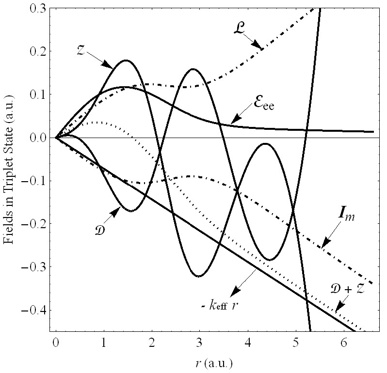
V ‘Quantal Newtonian’ First Law

For the triplet state of the quantum dot, the ‘Quantal Newtonian’ first law of Eq. (3) may be written in terms of the individual fields, binding $\omega_{0}$ and Larmor $\omega_{L}$ frequencies , and the effective force constant $k_{\mathrm{eff}}$ as

$$-k_{\mathrm{eff}}r = -[\omega^{2}_{0}+\omega^{2}_{L}]r$$ (54)

$$= -\omega^{2}_{0}r-[{\boldsymbol{\cal{L}}}({\bf{r}})+{\boldsymbol{\cal{I}}}_{m}({\bf{r}})]=-{\boldsymbol{\cal{E}}}_{ee}({\bf{r}})+{\boldsymbol{\cal{Z}}}({\bf{r}})+{\boldsymbol{\cal{D}}}({\bf{r}}).$$ (55)

These fields are plotted in Fig. 18. In the figure, the Lorentz ${\boldsymbol{\cal{L}}}({\bf{r}})$ and internal magnetic ${\boldsymbol{\cal{I}}}_{m}({\bf{r}})$ fields, which are the only two fields that depend on the magnetic field, are drawn for $\omega_{L}=0.1$. As shown in Fig. 17, the singularities in these two fields cancel to lead to the linear function $\omega_{L}^{2}r$. The singularities in the differential density ${\boldsymbol{\cal{D}}}({\bf{r}})$ and kinetic ${\boldsymbol{\cal{Z}}}({\bf{r}})$ fields also cancel to lead to a linear function (see plot of ${\boldsymbol{\cal{D}}}({\bf{r}})+{\boldsymbol{\cal{Z}}}({\bf{r}})$ in Fig. 18). On the addition of the electron-interaction field $-{\boldsymbol{\cal{E}}}_{ee}({\bf{r}})$ to ${\boldsymbol{\cal{D}}}({\bf{r}})+{\boldsymbol{\cal{Z}}}({\bf{r}})$, one obtains the linear function $-k_{\mathrm{eff}}r$. This then demonstrates the satisfaction of the ‘Quantal Newtonian’ first law by the various fields experienced by each electron.

VI Self-Consistent Nature of the Schrödinger-Pauli Equation

The example of the triplet state of the quantum dot in a magnetic field can be employed to demonstrate the intrinsic self-consistent nature of the Schrödinger-Pauli equation. Consider the Schrödinger-Pauli equation for the quantum dot written in its generalized form (See Part I) (in effective atomic units)

$$\hat{H}[\Psi]\Psi=E[\Psi]\Psi,$$ (56)

where the Hamiltonian $\hat{H}[\Psi]$ with unknown binding potential $v[\Psi]({\bf{r}})$ is

$$\hat{H}[\Psi]=\frac{1}{2}\sum^{2}_{k=1}\big{(}{\bf{p}}_{k}+{\bf{A}}({\bf{r}}_{k})\big{)}^{2}+\sum^{2}_{k=1}{\bf{B}}({\bf{r}}_{k})\cdot{\bf{s}}_{k}+\frac{1}{2}\sideset{}{{}^{\prime}}{\sum}_{k,\ell=1}^{2}\frac{1}{|{\bf{r}}_{k}-{\bf{r}}_{\ell}|}+\sum^{2}_{k=1}v[\Psi]({\bf{r}}_{k}),$$ (57)

with

$$v[\Psi]({\bf{r}})=\int^{\bf{r}}_{\infty}\big{[}{\boldsymbol{\cal{E}}}_{\mathrm{ee}}({\bf{r}}^{\prime})-{\boldsymbol{\cal{D}}}({\bf{r}}^{\prime})-{\boldsymbol{\cal{Z}}}({\bf{r}}^{\prime})-{\boldsymbol{\cal{L}}}({\bf{r}}^{\prime})-{\boldsymbol{\cal{I}}}_{m}({\bf{r}}^{\prime})\big{]}\cdot d{\boldsymbol{\ell}}^{\prime}.$$ (58)

(The above equations are written in terms of the spatial part $\Psi({\bf{r}}_{1}{\bf{r}}_{2})$ of the wave function.) In the symmetric gauge ${\bf{A}}({\bf{r}})=\frac{1}{2}{\boldsymbol{\cal{B}}}({\bf{r}})\times{\bf{r}}$ ; ${\boldsymbol{\cal{B}}}({\bf{r}})={\cal{B}}{\bf{i}}_{z}$, with the assumption of cylindrical symmetry, let us assume the form of a trial input wave function to be

$$\Psi({\bf{r}}_{1}{\bf{r}}_{2})=Ne^{im\theta}e^{-\Omega(R^{2}+\frac{1}{4}u^{2})}\big{[}u+c_{2}u^{2}+c_{3}u^{3}+c_{4}u^{4}\big{]}$$ (59)

where ${\bf{r}}=({\bf{r}}_{1}+{\bf{r}}_{2})/2~{};~{}{\bf{u}}=|{\bf{r}}_{2}-{\bf{r}}_{1}|$; the angular momentum quantum number $m=1$; the Larmor frequency $\omega_{L}=0.1$; and $N,\Omega\equiv\sqrt{k_{\mathrm{eff}}},c_{2},c_{3},c_{4}$ are unknown constants. As a consequence of cylindrical symmetry, let us assume all the individual fields are conservative.

For an assumed choice of the values of the constants, employ the input $\Psi({\bf{r}}_{1}{\bf{r}}_{2})$ to determine the various fields, and from them the potential $v[\Psi]({\bf{r}})$. Substitute this $v[\Psi]({\bf{r}})$ into Eq. (56) to solve for $\Psi({\bf{r}}_{1}{\bf{r}}_{2})$ with new coefficients, and repeat the iterative procedure. At each iteration one also obtains the corresponding $E[\Psi]$. (We reiterate that what is meant by the functional $v[\Psi]({\bf{r}})$ is that for each different $\Psi$, one obtains a different function $v[\Psi]({\bf{r}})$.)

Suppose at the end of a particular iteration, the values of the coefficients turn out to be $N=0.022466$, $c_{2}=0.33333$, $c_{3}=-0.059108$, $c_{4}=-0.015884$; $\Omega^{2}\equiv k_{\mathrm{eff}}=0.072217$. On substituting the $v({\bf{r}})$ of Eq. (58) into the Schrödinger-Pauli equation Eq. (56) and solving, one obtains a wave function $\Psi({\bf{r}}_{1}{\bf{r}}_{2})$ with the same coefficients. Thus, this constitutes the final iteration of the self-consistent procedure, thereby leading to the exact wave function $\Psi({\bf{r}}_{1}{\bf{r}}_{2})$ and energy $E$. Hence, via the self-consistency procedure one obtains the Hamiltonian, the wave function, and eigen energy.

An examination of the final result of the sum of $-{\boldsymbol{\cal{E}}}_{\mathrm{ee}}({\bf{r}})$, ${\boldsymbol{\cal{D}}}({\bf{r}})$, and ${\boldsymbol{\cal{Z}}}({\bf{r}})$ fields will show it to be a linear function of slope $-k_{\mathrm{eff}}=-0.072217$ (see Fig. 18), as follows

$$-{\boldsymbol{\cal{E}}}_{\mathrm{ee}}({\bf{r}})+{\boldsymbol{\cal{D}}}({\bf{r}})+{\boldsymbol{\cal{Z}}}({\bf{r}})=-k_{\mathrm{eff}}r.$$ (60)

As the individual fields are conservative, the sum of the magnetic fields ${\boldsymbol{\cal{M}}}({\bf{r}})=-[{\boldsymbol{\cal{L}}}({\bf{r}})+{\boldsymbol{\cal{I}}}_{m}({\bf{r}})]$ is such that ${\boldsymbol{\nabla}}\times{\boldsymbol{\cal{M}}}({\bf{r}})=0$. Then these fields can be associated with a magnetic scalar potential $v_{m}({\bf{r}})$ through

$$v_{m}[\Psi]({\bf{r}})=-\int^{\bf{r}}_{\infty}{\boldsymbol{\cal{M}}}({\bf{r}}^{\prime})\cdot d{\boldsymbol{\ell}}^{\prime}.$$ (61)

As such, Eq. (58) can be rearranged to read

$$v[\Psi]({\bf{r}})+v_{m}[\Psi]({\bf{r}}) \equiv v_{\mathrm{eff}}[\Psi]({\bf{r}})$$ (62)

$$= \int^{\bf{r}}_{\infty}\big{[}{\boldsymbol{\cal{E}}}_{\mathrm{ee}}({\bf{r}}^{\prime})-{\boldsymbol{\cal{D}}}({\bf{r}}^{\prime})-{\boldsymbol{\cal{Z}}}({\bf{r}}^{\prime})\big{]}\cdot d{\boldsymbol{\ell}}^{\prime}.$$

On substituting Eq. (60) in Eq. (62) the effective potential $v_{\mathrm{eff}}({\bf{r}})$ turns out to be harmonic as

$$v_{\mathrm{eff}}({\bf{r}})=\frac{1}{2}k_{\mathrm{eff}}r^{2},$$ (63)

with $k_{\mathrm{eff}}$ as given above.

A further examination of the final result of the field ${\boldsymbol{\cal{M}}}({\bf{r}})$ shows that the corresponding magnetic scalar potential $v_{m}({\bf{r}})$ is also harmonic with Larmor frequency $\omega_{L}=0.1$ as

$$v_{m}({\bf{r}})=\frac{1}{2}\omega^{2}_{L}r^{2}.$$ (64)

Consequently, since both $v_{\mathrm{eff}}({\bf{r}})$ and $v_{m}({\bf{r}})$ are harmonic, their difference which is the binding external electrostatic potential $v({\bf{r}})$, must also be harmonic, with some angular frequency $\omega_{0}$ as

$$v({\bf{r}})=\frac{1}{2}\omega^{2}_{0}r^{2},$$ (65)

where $\omega^{2}_{0}=k_{\mathrm{eff}}-\omega^{2}_{L}=0.062217$. Thus, via the self-consistent procedure, the unknown external potential $v({\bf{r}})$ is determined to be harmonic. (Note that for a different value of the magnetic field ${\boldsymbol{\cal{B}}}({\bf{r}})$ or equivalently Larmor frequency $\omega_{L}$, one would also obtain a $v({\bf{r}})$ that is harmonic, but with a different angular frequency $\omega_{0}$. However, the value of the effective force constant $k_{\mathrm{eff}}$ will remain unchanged.)

VII Concluding Remarks

The purpose of this paper is to demonstrate by example the new perspective of Schrödinger-Pauli theory of electrons explained in Part I. The perspective complements the traditional description of quantum mechanics in that it leads to a deeper understanding of the physical system. The perspective is that of the individual electron via its equation of motion, or equivalently, in the stationary state case, the ‘Quantal Newtonian’ first law. The law is in terms of ‘classical’ fields whose sources are quantum-mechanical expectation values of Hermitian operators taken with respect to the wave function. The structure of the quantal sources is predictive of the structure of the fields. One new insight obtained via the law is that in addition to the external fields, each electron also experiences an internal field. And this internal field is comprised of components that are representative of intrinsic properties of the system – the correlations due to the Pauli Exclusion Principle and Coulomb repulsion, the electronic density, kinetic effects, and an internal magnetic field component dependent on the electronic current density. Thus, in the presence of a magnetic field, not only does each electron experience a Lorentz field, but also an internal magnetic field. It further experiences a kinetic field. The total energy and its components can also be described in terms of these fields. The field description makes for an understanding of the quantum system that is tangible. As explained in Part I, the fields are deterministic. The sources of these fields are probabilistic in that they are quantum-mechanical expectation values. The quantal sources are both local and nonlocal, and that is why one must first determine fields from which then potentials and energies can be obtained. These new understandings then enhance the traditional quantum-mechanical description of a physical system.

A second new understanding is that all the quantal sources and fields are related to each other in a self-consistent manner. This is because as shown in Part I, the Schrödinger-Pauli equation can be written in a generalized form in terms of the various fields descriptive of the system. Written in this manner, it shows the Schrödinger-Pauli equation to be an intrinsically self-consistent one. This then provides a self-consistent procedure for the solution of the Schrödinger-Pauli equation.

The quantal-source – field perspective of the Schrödinger-Pauli theory via the ‘Quantal Newtonian’ first law is applied in this work to the triplet $2^{3}S$ state of a $2$-dimensional $2$-electron quantum dot in a magnetic field. The purpose of the application is to demonstrate each facet of the new formalism. Hence, we first study the local quantal sources of the density $\rho({\bf{r}})$, and the current density ${\bf{j}}({\bf{r}})$ and its paramagnetic ${\bf{j}}_{p}({\bf{r}})$, diamagnetic ${\bf{j}}_{d}({\bf{r}})$, and magnetization ${\bf{j}}_{m}({\bf{r}})$ components, and their circulation; and then the nonlocal sources of the pair-correlation density $g({\bf{rr}}^{\prime})$, the Fermi-Coulomb hole charge distribution $\rho_{\mathrm{xc}}({\bf{rr}}^{\prime})$, and the single-particle density matrix $\gamma({\bf{rr}}^{\prime})$. These sources give rise to fields experienced by each electron: the electron-interaction field ${\boldsymbol{\cal{E}}}_{\mathrm{ee}}({\bf{r}})$ and its Hartree ${\boldsymbol{\cal{E}}}_{H}({\bf{r}})$ and Pauli-Coulomb ${\boldsymbol{\cal{E}}}_{\mathrm{xc}}({\bf{r}})$ components; the kinetic field ${\boldsymbol{\cal{Z}}}({\bf{r}})$; the differential density field ${\boldsymbol{\cal{D}}}({\bf{r}})$; the Lorentz ${\boldsymbol{\cal{L}}}({\bf{r}})$ and internal magnetic ${\boldsymbol{\cal{I}}}_{m}({\bf{r}})$ fields. These fields exhibit characteristics of the system such as shell structure. They satisfy the ‘Quantal Newtonian’ first law. Together with the external electrostatic field ${\boldsymbol{\cal{E}}}({\bf{r}})$, these fields then give rise to the components of the total energy: the electron-interaction $E_{\mathrm{ee}}$, Hartree $E_{H}$, Pauli-Coulomb $E_{\mathrm{xc}}$, kinetic $T$, the external electrostatic $E_{\mathrm{es}}$, and the magnetostatic $E_{\mathrm{mag}}$ with $E_{\mathrm{mag}}$ the sum of the Lorentz and internal magnetic energy.

Finally, the example allows for the demonstration of the self-consistency procedure of the Schrödinger-Pauli equation. Thus, it is shown how in the last iteration of the self-consistent procedure, the exact wave function, eigen energy, and the external binding potential and therefore the Hamiltonian are determined.

Appendix A Expressions for Properties of the Triplet $2^{3}S$ State of a Two-Electron Quantum Dot in a Magnetic Field

In this Appendix we provide the closed-form analytical and semi-analytical expressions for various properties of the $2^{3}S$ state of the quantum dot in a magnetic field. In these expressions the zeroth​- and first-order modified Bessel functions $I_{0}(x)$ and $I_{1}(x)$ appear. The general Bessel function $I_{\nu}(x)$ is defined as 23

$$I_{\nu}(x)=\sum_{n=0}^{\infty}\frac{1}{n!\Gamma(n+\nu+1)}\bigg{(}\frac{1}{2}x\bigg{)}^{2n+\nu},$$ (66)

where the Gamma function $\Gamma(n)$ is 23

$$\Gamma(n)=\int^{\infty}_{0}t^{n-1}e^{-t}dt~{}~{};~{}~{}n>0.$$ (67)

Also the parameter $\Omega$ is related to the binding frequency $\omega_{0}$, the Larmor frequency $\omega_{L}$, and the effective force constant $k_{\mathrm{eff}}$ as

$$\Omega=\sqrt{k_{\mathrm{eff}}}=\sqrt{\omega^{2}_{0}+\omega^{2}_{L}}=0.268732$$ (68)

Other constants that appear in the expressions are

$$A = \frac{1}{3}~{};~{}B=\frac{1}{8}(\frac{1}{3}-3\Omega)=-0.059108$$

$$C = \frac{1}{360}(1-25\Omega)=-0.015884.$$ (69)

Electron density $\rho({\bf r})$

$$\rho(\emph{r})=4\pi N^{2}e^{-2\Omega r^{2}}\int^{\infty}_{0}e^{-\Omega x^{2}}x\big{[}x+c_{2}x^{2}+c_{3}x^{3}+c_{4}x^{4}\big{]}^{2}I_{0}(2\Omega rx)dx$$

$$=\frac{N^{2}}{4\Omega^{9}}\bigg{\{}8\pi\Omega^{4}e^{-\Omega r^{2}}\big{(}K_{1}+L_{1}r^{2}+M_{1}r^{4}+N_{1}r^{6}+O_{1}r^{8}\big{)}+$$

$$\pi^{3/2}\Omega^{9/2}\ e^{-\frac{3}{2}\Omega r^{2}}\bigg{[}K_{2}+L_{2}r^{2}+M_{2}r^{4}+N_{2}r^{6}+O_{2}r^{8}\big{)}\ I_{o}\big{(}\Omega r^{2}/2\big{)}+$$

$$2\Omega\big{(}L_{3}r^{2}+M_{3}r^{4}+N_{3}r^{6}+O_{3}r^{8}\big{)}\ I_{1}\big{(}\Omega r^{2}/2\big{)}\bigg{]}\bigg{\}},$$ (70)

where

$$\ N = 0.02246632108,$$

$$\ K_{1} = 24C^{2}+(6B^{2}+12AC)\ \Omega+2A^{2}\ \Omega^{2},$$

$$L_{1} = 96\ C^{2}\ \Omega+(18B^{2}+36AC)\ \Omega^{2}+(4A^{2}+8B)\ \Omega^{3}+\Omega^{4},$$

$$M_{1} = 2\ C^{2}\ \Omega^{2}+(9B^{2}+18AC)\ \Omega^{3}+(A^{2}+2B)\ \Omega^{4},$$

$$N_{1} = 16\ C^{2}\ \Omega^{3}+(B^{2}+2AC)\ \Omega^{4},$$

$$O_{1} = C^{2}\ \Omega^{4},$$

$$K_{2} = 105BC+30(AB+C)\ \Omega+12A\ \Omega^{2},$$

$$L_{2} = 420BC\ \Omega+90(AB+C)\ \Omega^{2}+24A\ \Omega^{3},$$

$$M_{2} = 376BC\ \Omega^{2}+56(AB+C)\ \Omega^{3}+8A\ \Omega^{4},$$

$$N_{2} = 104BC\ \Omega^{3}+8(AB+C)\ \Omega^{4},$$

$$O_{2} = 8BC\ \Omega^{4},$$

$$L_{3} = 88BC+23(AB+C)\ \Omega+8A\ \Omega^{2},$$

$$M_{3} = 142BC\ \Omega+24(AB+C)\ \ \Omega^{2}+4A\ \Omega^{3},$$

$$N_{3} = 48BC\ \Omega^{2}+4(AB+C)\ \Omega^{3},$$

$$O_{3} = 4BC\ \Omega^{3}.$$ (71)

The asymptotic structure of $\rho(\bf{r})$ near the center of the quantum dot, and in the classically forbidden region, respectively, is as follows:

$$\rho(r)\ \begin{subarray}{c}\ \\ \\ \sim\\ {r\to 0}\end{subarray}\ 0.0555-0.00625\ r^{2}-0.000230\ r^{4}+\ldots$$ (72)

with $\rho(0)=0.0555377\ a.u.$,

$$\rho(r)\ \begin{subarray}{c}\ \\ \\ \sim\\ {r\to\infty}\end{subarray} e^{-\Omega r^{2}}\ 10^{-5}\ (8.03\ r^{4}+12.6\ r^{5}+9.35\ r^{6}+2.22\ r^{7}+0.298\ r^{8}+\ldots)$$ (73)

Physical current density ${\bf{j}}({\bf r})$ and its components

$${\bf{j}}({\bf r})={\bf{j}}_{p}({\bf r})+{\bf{j}}_{d}({\bf r})+{\bf{j}}_{m}({\bf r}),$$ (74)

where ${\bf{j}}_{p}({\bf r}),{\bf{j}}_{d}({\bf r})$, and ${\bf{j}}_{m}({\bf r})$ are the paramagnetic, diamagnetic and magnetization current density components, respectively. The components are

$${\bf{j}}_{p}({\bf r})=j_{p}(r)~{}\hat{\bf{i}}_{\theta}=\bigg{\{}\frac{2\pi}{\Omega}N^{2}e^{-2\Omega r^{2}}$$

$$\frac{\partial}{\partial r}\bigg{[}\int^{\infty}_{0}e^{-\Omega x^{2}}\frac{1}{x}\bigg{(}x+c_{2}x^{2}+c_{3}x^{3}+c_{4}x^{4}\bigg{)}^{2}I_{0}(2\Omega rx)dx\bigg{]}\bigg{\}}~{}\hat{\bf{i}}_{\theta}$$

$$=\frac{\pi N^{2}e^{-3\Omega r^{2}/2}}{4\Omega^{4}}\bigg{\{}8e^{\Omega r^{2}/2}\bigg{[}\bigg{(}24C^{2}+(6B^{2}+12AC)\Omega+(2A^{2}+4B)\Omega^{2}+\Omega^{3}\bigg{)}r+$$

$$\bigg{(}36C^{2}\Omega+(6B^{2}+12AC)\Omega^{2}+(A^{2}+2B)\Omega^{3}\bigg{)}r^{3}+\bigg{(}12C^{2}\Omega^{2}+(B^{2}+2AC)\Omega^{3}\bigg{)}r^{5}+$$

$$C^{2}\Omega^{3}r^{7}+\sqrt{\pi\Omega}\bigg{[}\bigg{(}105BC+30(AB+C)\Omega+12A\Omega^{2}\bigg{)}r+\bigg{(}180BC\Omega+36(AB+$$

$$C)\Omega^{2}++8A\Omega^{3}\bigg{)}r^{3}+\bigg{(}76BC\Omega^{2}+8(AB+C)\Omega^{3}\bigg{)}r^{5}+8BC\Omega^{3}r^{7}\bigg{]}I_{0}(\Omega r^{2}/2)+$$

$$\sqrt{\pi\Omega}\bigg{[}\bigg{(}15BC+6(AB+C)\Omega+4A\Omega^{2}\bigg{)}r+\bigg{(}116BC\Omega+28(AB+C)\Omega^{2}+$$

$$8A\Omega^{3}\bigg{)}r^{3}+\bigg{(}68BC\Omega^{2}+8(AB+C)\Omega^{3}\bigg{)}r^{5}+8BC\Omega^{3}r^{7}\bigg{]}I_{1}(\Omega r^{2}/2)\bigg{\}}~{}\hat{\bf{i}}_{\theta},$$ (75)

$${\bf{j}}_{d}({\bf r})=j_{d}(r)~{}\hat{\bf{i}}_{\theta}=r\ \omega_{L}\ \rho(r)~{}\hat{\bf{i}}_{\theta},$$ (76)

$${\bf{j}}_{m}({\bf r})=j_{m}(r)~{}\hat{\bf{i}}_{\theta}=-\frac{1}{2}\ \frac{\partial\rho(r)}{\partial r}~{}\hat{\bf{i}}_{\theta}.$$ (77)

The asymptotic structures of ${\bf{j}}(\bf{r})$, and its components are

$${\bf{j}}({\bf r})\ \begin{subarray}{c}\ \\ \\ \sim\\ {r\to\ 0}\end{subarray}\ 0.0267\ r-0.00501\ r^{3}-0.0000511\ r^{5},$$

$${\bf{j}}({\bf r})\ \begin{subarray}{c}\ \\ \\ \sim\\ {r\to\infty}\end{subarray}\ e^{-\Omega r^{2}}10^{-6}\ (1.10\ r^{9}+8.17\ r^{8}+25.6\ r^{7}),$$

$${\bf{j}}_{p}({\bf r})\ \begin{subarray}{c}\ \\ \\ \sim\\ {r\to\ 0}\end{subarray}\ 0.0149\ r-0.00485\ r^{3}+0.000848\ r^{5},$$

$${\bf{j}}_{p}({\bf r})\ \begin{subarray}{c}\ \\ \\ \sim\\ {r\to\infty}\end{subarray}\ e^{-\Omega r^{2}}10^{-3}\ (0.00298\ r^{7}+0.0222\ r^{6}+0.049\ r^{5}-0.118\ r^{4}),$$

$${\bf{j}}_{d}({\bf r})\ \begin{subarray}{c}\ \\ \\ \sim\\ {r\to\ 0}\end{subarray}\ 10^{-3}\ (5.55\ r-0.625\ r^{3}-0.0230\ r^{5}),$$

$${\bf{j}}_{d}({\bf r})\ \begin{subarray}{c}\ \\ \\ \sim\\ {r\to\infty}\end{subarray}\ e^{-\Omega r^{2}}10^{-6}\ (0.298\ r^{9}+2.22\ r^{8}+9.35\ r^{7}+17.0\ r^{6}),$$

$${\bf{j}}_{m}({\bf r})\ \begin{subarray}{c}\ \\ \\ \sim\\ {r\to\ 0}\end{subarray}\ 10^{-3}\ (6.25\ r+0.461\ r^{3}-0.876\ r^{5}),$$

$${\bf{j}}_{m}({\bf r})\ \begin{subarray}{c}\ \\ \\ \sim\\ {r\to\infty}\end{subarray}\ e^{-\Omega r^{2}}10^{-5}\ (0.0800\ r^{9}+0.596\ r^{8}+1.32\ r^{7}).$$ (78)

Pair-correlation density $g({\bf rr}^{\prime})$

$$g({\bf rr^{\prime}})=\frac{2\ N^{2}\ e^{-\Omega(r^{2}+{r^{\prime}}\ ^{2})}\ \bigg{[}|{\bf r}-{\bf r^{\prime}}|+A\ |{\bf r}-{\bf r^{\prime}}|^{2}+B|{\bf r}-{\bf r^{\prime}}|^{3}+C|{\bf r}-{\bf r^{\prime}}|^{4}\bigg{]}^{2}}{\rho({\bf r})}.$$ (79)

Single-particle density matrix $\gamma({\bf rr^{\prime}})$

$$\gamma({\bf rr^{\prime}})=2\ N^{2}\ e^{-\Omega(r^{2}+{r^{\prime}}\ ^{2})/2}\int e^{-\Omega\ y^{2}}\ \bigg{[}|{\bf y}-{\bf r}|+A|{\bf y}-{\bf r}|^{2}+$$

$$B|{\bf y}-{\bf r}\big{|}^{3}+C|{\bf y}-{\bf r}\big{|}^{4}\bigg{]}\bigg{[}|{\bf y}-{\bf r^{\prime}}|+A|{\bf y}-{\bf r^{\prime}}|^{2}+B|{\bf y}-{\bf r^{\prime}}\big{|}^{3}+C|{\bf y}-{\bf r^{\prime}}\big{|}^{4}\bigg{]}\ d{\bf y}.$$ (80)

Electron-interaction field $\boldsymbol{\cal{E}}_{ee}({\bf r})$

$$\boldsymbol{\cal{E}}_{ee}({\bf r})=\frac{4\ \pi\ N^{2}}{32\ \Omega^{7/2}\rho(\bf{r})}\bigg{\{}\sqrt{\pi}\ e^{-3\Omega r^{2}/2}\bigg{[}I_{1}\big{(}\Omega\ r^{2}/2\big{)}\ \bigg{(}\big{[}15C^{2}+\big{(}6B^{2}+12AC\big{)}\Omega+$$

$$\big{(}4A^{2}+8B\big{)}\Omega^{2}+8\Omega^{3}\big{]}r+\big{[}116C^{2}\ \Omega+\big{(}28B^{2}+56AC\big{)}\ \Omega^{2}+\big{(}8A^{2}+$$

$$16B\big{)}\ \Omega^{3}\ \big{]}r^{3}+\big{[}68C^{2}\ \Omega^{2}+\big{(}8B^{2}+16AC\big{)}\ \Omega^{3}\big{]}r^{5}+8C^{2}\ \Omega^{3}\ r^{7}\bigg{)}+$$

$$I_{0}\big{(}\Omega\ r^{2}/2\big{)}\ \bigg{(}\big{[}105C^{2}+\big{(}30B^{2}+60AC\big{)}\ \Omega+\big{(}12A^{2}+24AB\big{)}\ \Omega^{2}+$$

$$8\ \Omega^{3}\big{]}r+\big{[}180C^{2}\ \Omega+\big{(}36B^{2}+72AC\big{)}\ \Omega^{2}+\big{(}8A^{2}+16B\big{)}\ \Omega^{3}\big{]}r^{3}+$$

$$\big{[}76C^{2}\ \Omega^{2}+\big{(}8B^{2}+16AC\big{)}\ \Omega^{3}\big{]}r^{5}+8C^{2}\ \Omega^{3}r^{7}\bigg{)}\ \bigg{]}+32\sqrt{\Omega}\ e^{-\Omega r^{2}}\bigg{[}\ \bigg{(}6BC+$$

$$\big{(}2AB+2C\big{)}\ \Omega+A\ \Omega^{2}\bigg{)}r+\bigg{(}6BC\ \Omega+\big{(}AB+C\big{)}\ \Omega^{2}\bigg{)}r^{3}+BC\ \Omega^{2}r^{5}\bigg{]}\ \bigg{\}},$$ (81)

The asymptotic structure of $\boldsymbol{\cal{E}}_{\mathrm{ee}}(\bf{r})$ and its Hartree ${\boldsymbol{\cal{E}}}_{H}({\bf{r}})$, and Pauli-Coulomb ${\boldsymbol{\cal{E}}}_{xc}({\bf{r}})$ components is

$${\cal E}_{ee}(r) \ \begin{subarray}{c}\ \\ \\ \sim\\ {r\to\ 0}\end{subarray}\ 0.137\ r-0.0360\ r^{3},\ \ \ \ \ \ \ \ {\cal E}_{ee}(r)\ \begin{subarray}{c}\ \\ \\ \sim\\ {r\to\infty}\end{subarray}\ \frac{1}{r^{2}}-\frac{0.0754}{r^{3}}-\frac{24.0}{r^{4}},$$ (82)

$${\cal E}_{H}(r) \ \begin{subarray}{c}\ \\ \\ \sim\\ {r\to\infty}\end{subarray}\ \frac{2}{r^{2}}-\frac{0.0287}{r^{3}}+\frac{16.3}{r^{4}},\ \ \ \ \ \ \ \ {\cal E}_{xc}(r)\ \begin{subarray}{c}\ \\ \\ \sim\\ {r\to\infty}\end{subarray}\ -\frac{1}{r^{2}}-\frac{0.0467}{r^{3}}-\frac{40.3}{r^{4}}.$$

Electron-interaction energy $E_{ee}$

$$E_{ee}=\pi^{2}N^{2}\bigg{\{}\frac{4}{\Omega^{5}}\big{[}24BC+4\big{(}AB+C\big{)}\Omega+A\ \Omega^{2}\big{]}+\big{[}105C^{2}+$$

$$15\big{(}B^{2}+2AC)\ \Omega+3\big{(}A^{2}+2AB)\Omega^{2}+\ \Omega^{3}\big{]}\bigg{\}}=0.254158\ (a.u.)^{\star}.$$ (83)

Kinetic energy tensor $t_{\alpha\beta}[{\bf r;\gamma}]$

$$t_{\alpha\beta}[{\bf r;\gamma}]=\frac{r_{\alpha}\ r_{\beta}}{r^{2}}\ f(r)+\delta_{\alpha\beta}\ k(r),$$ (84)

where

$$f(r)=\pi\ N^{2}e^{-2\Omega r^{2}}\bigg{[}\frac{r}{\Omega}\frac{\partial f_{1}(r)}{\partial r}-2\ r\frac{\partial f_{2}(r)}{\partial r}\bigg{]}+\frac{\Omega^{2}}{2}\ r^{2}\rho(r),$$ (85)

$$k(r)=\pi\ N^{2}\ e^{-2\Omega r^{2}}\bigg{[}\frac{f_{1}(r)}{\Omega}+2f_{3}(r)\bigg{]},$$ (86)

$$f_{1}(r)=\frac{e^{\Omega r^{2}/2}}{8\ \Omega^{3}}\bigg{\{}4\ e^{\Omega^{2}r^{2}/2}\bigg{[}\ \bigg{(}90C^{2}\ \Omega+\big{(}8B^{2}+14AC\big{)}\Omega^{2}\bigg{)}\big{(}1+r^{2}\big{)}+15C^{2}\ \Omega^{2}r^{4}\bigg{]}+$$

$$\sqrt{\pi\Omega}\bigg{[}\bigg{(}165BC+\big{(}30AB+18C\big{)}\Omega+4A\ \Omega^{2}\bigg{)}+r^{2}\bigg{(}198BC\ \Omega+\big{(}20AB+$$

$$12C\big{)}\Omega^{2}\bigg{)}+44BC\Omega^{2}r^{4}\bigg{]}I_{0}(\Omega r^{2}/2)+\sqrt{\pi\Omega}\ \bigg{[}\bigg{(}33BC+\big{(}10AB+6C\big{)}\Omega+$$

$$4A\Omega^{2}\bigg{)}+r^{2}\bigg{(}154BC\Omega+\big{(}20AB+12C\big{)}\Omega^{2}\bigg{)}+44BC\Omega^{2}r^{4}\bigg{]}I_{1}(\Omega r^{2}/2)\bigg{\}}$$ (87)

$$f_{2}(r)=\frac{e^{\Omega r^{2}/2}}{16\Omega^{4}}\bigg{\{}8e^{\Omega r^{2}/2}\bigg{[}\bigg{(}24C^{2}+\big{(}6B^{2}+12AC\big{)}\Omega+\big{(}2A^{2}+4B\big{)}\Omega^{2}+\Omega^{3}\bigg{)}+$$

$$\bigg{(}72C^{2}\Omega+\big{(}12B^{2}+24AC\big{)}\Omega^{2}+\big{(}2A^{2}+4B\big{)}\Omega^{3}\bigg{)}r^{2}+\bigg{(}36C^{2}\Omega^{2}+\big{(}3B^{2}+$$

$$6AC\big{)}\Omega^{3}\bigg{)}r^{4}+4C^{2}\Omega^{3}r^{6}\bigg{]}+\sqrt{\pi\Omega}\bigg{[}\bigg{(}105BC+30\big{(}AB+C)\Omega+12A\Omega^{2}\bigg{)}+$$

$$28BC\Omega^{3}r^{6}+\bigg{(}315BC\Omega+60\big{(}AB+C\big{)}\Omega^{2}+12A\Omega^{3}\bigg{)}r^{2}+\bigg{(}196BC\Omega^{2}+$$

$$20\big{(}AB+C\big{)}\Omega^{3}\bigg{)}r^{4}\bigg{]}I_{0}(\Omega r^{2}/2)+\sqrt{\pi\Omega}\ \Omega\bigg{[}\bigg{(}161BC+40\big{(}AB+C\big{)}\Omega+$$

$$12A\Omega^{2}\bigg{)}r^{2}+\bigg{(}168BC\Omega+20\big{(}AB+C\big{)}\Omega^{2}\bigg{)}r^{4}+28BC\Omega^{2}r^{6}\bigg{]}I_{1}(\Omega r^{2}/2)\bigg{\}}$$ (88)

$$f_{3}(r)=\frac{e^{\Omega r^{2}/2}}{8\Omega^{4}}\bigg{\{}4e^{\Omega r^{2}/2}\bigg{[}\bigg{(}6C^{2}+2\big{(}2B^{2}+4AC\big{)}\Omega+(A^{2}+2B\big{)}\Omega^{2}+\Omega^{3}\bigg{)}+$$

$$\bigg{(}18C^{2}\Omega+4(B^{2}+2AC)\Omega^{2}+(A^{2}+2B)\Omega^{3}\bigg{)}r^{2}+\bigg{(}9C^{2}\Omega^{2}+(B^{2}+$$

$$2AC)\Omega^{3}\bigg{)}r^{4}+C^{2}\Omega^{3}r^{6}\bigg{]}+\sqrt{\pi\Omega}\bigg{[}\bigg{(}15BC+6(AB+C)\Omega+4A\Omega^{2}\bigg{)}+$$

$$\bigg{(}45BC\Omega+12(AB+C)\Omega^{2}+4A\Omega^{3}\bigg{)}r^{2}+\bigg{(}28BC\Omega^{2}+4(AB+C)\Omega^{3}\bigg{)}r^{4}+$$

$$4BC\Omega^{3}r^{6}\bigg{]}I_{0}(\Omega r^{2}/2)+\sqrt{\pi\Omega}\ \Omega\bigg{[}\bigg{(}23BC+8(AB+C)\Omega+4A\Omega^{2}\bigg{)}r^{2}+$$

$$\bigg{(}24BC\Omega+4(AB+C)\Omega^{2}\bigg{)}r^{4}+4BC\Omega^{2}r^{6}\bigg{]}I_{1}(\Omega r^{2}/2)\bigg{\}}.$$ (89)

Kinetic ‘force’ $z_{\alpha}[\bf{r};\gamma]$

$$z_{\alpha}[{\bf r;\gamma}]=\frac{2\ r_{\alpha}}{r}\bigg{\{}\frac{\partial[f(r)+k(r)]}{\partial r}+\frac{f(r)}{r}\bigg{\}},$$ (90)

where the functions $f(r)$ and $k(r)$ are given in Eq. (A20) and (A21), respectively. The asymptotic structures are

$$z(r)\ \begin{subarray}{c}\ \\ \\ \sim\\ {r\to 0}\end{subarray}\ 0.00174\ r+0.00811\ r^{3}+\ldots$$ (91)

$$z(r)\ \begin{subarray}{c}\ \\ \\ \sim\\ {r\to\infty}\end{subarray}\ e^{-\Omega r^{2}}10^{-5}(-0.0116r^{11}-0.0860r^{10}+0.218r^{9}-0.0700r^{8}+5.55r^{7}+\ldots).$$ (92)

Kinetic Energy $T$

$$T=\frac{N_{R}^{2}\ \pi}{4}+\frac{N_{r}^{2}\ \pi}{\Omega^{4}}\bigg{(}480C^{2}+12A^{2}\Omega^{2}+3A\sqrt{\pi/2}\ \Omega^{3/2}(13B+3\Omega)+1.5C(85B\sqrt{2\pi\Omega}+$$

$$64A\Omega+5\sqrt{2\pi}\Omega^{3/2})+4\Omega(16B^{2}+4B\Omega+\Omega^{2})\bigg{)}=0.615577~{}(a.u.)^{\star},$$ (93)

where $N_{r}=0.05431655771,N_{R}=0.4136182782$.

Lorentz ${\boldsymbol{\cal{L}}}({\bf{r}})$ and Internal Magnetic ${\boldsymbol{\cal{I}}}_{m}({\bf{r}})$ Fields

$${\boldsymbol{\cal{L}}}({\bf{r}})=\frac{2\omega_{L}j(r)}{\rho(r)}~{}\hat{\bf{i}}_{r},$$ (94)

$${\boldsymbol{\cal{I}}}_{m}({\bf{r}})=\bigg{[}-\frac{2\omega_{L}j(r)}{\rho(r)}+\omega^{2}_{L}r\bigg{]}~{}\hat{\bf{i}}_{r},$$ (95)

$${\boldsymbol{\cal{M}}}({\bf{r}})=-[{\boldsymbol{\cal{L}}}({\bf{r}})+{\boldsymbol{\cal{I}}}_{m}({\bf{r}})]=-\omega^{2}_{L}r~{}{\bf{i}}_{r},$$ (96)

where $j(r)=j_{p}(r)+j_{d}(r)+j_{m}(r)$ (see Eqs. (A10-A12).)

External Electrostatic $E_{es}$ and Magnetostatic $E_{mag}$ Energies

$$E_{es}+E_{mag} = \int\rho(r)\bigg{[}\frac{1}{2}k_{\mathrm{eff}}r^{2}\bigg{]}d{\bf{r}}$$ (97)

$$= k_{\mathrm{eff}}\frac{\pi^{2}N^{2}}{4\Omega^{7}}\bigg{(}64\Omega^{2}\ (A^{2}+2B)+480\Omega(2AC+B^{2})+135\sqrt{2\pi}\ \Omega^{3/2}(AB+C)$$

$$+ \sqrt{2\pi\Omega}\ (21A\Omega^{2}+1155BC)+4608C^{2}+12\Omega^{3}\bigg{)}$$

$$= 0.742657~{}(a.u.)^{\star}$$

Expectation values

With the complete elliptical integrals 23

$$K(p) = \int^{\pi/2}_{0}\frac{d\theta}{\sqrt{1-p^{2}\sin^{2}\theta}},$$ (98)

$$E(p) = \int^{\pi/2}_{0}\sqrt{1-p^{2}\sin^{2}\theta}d\theta,$$ (99)

the expressions and values of the various expectations are:

$$<r>=\int\rho(r)\ r\ d{\bf r}$$

$$=\frac{\pi^{2}N^{2}}{2\Omega^{13/2}}\bigg{[}\frac{47}{2}\sqrt{\pi}\ \Omega^{2}(A^{2}+2B)+\frac{639}{4}\sqrt{\pi}\ \Omega(2AC+B^{2})+\sqrt{2}\ \Omega^{3/2}\bigg{(}174E(1/2)-$$

$$47K(1/2)\bigg{)}(AB+C)+2\sqrt{2}\ A\Omega^{5/2}\bigg{(}15E(1/2)-4K(1/2)\bigg{)}+5\sqrt{2\Omega}\ BC$$

$$\bigg{(}273E(1/2)-74K(1/2)\bigg{)}+\frac{11313}{8}\sqrt{\pi}\ C^{2}+5\sqrt{\pi}\ \Omega^{3}\bigg{]}=5.823553\ (a.u.)^{\star},$$ (100)

$$<r^{2}>=\int\rho(r)\ r^{2}\ d{\bf r}$$

$$=\frac{\pi^{2}N^{2}}{2\Omega^{7}}\bigg{(}4608C^{2}+1155BC\sqrt{2\pi\Omega}+480(B^{2}+2AC)\Omega+135(AB+$$

$$C)\sqrt{2\pi}\Omega^{3/2}+64(A^{2}+2B)\Omega^{2}+21A\sqrt{2\pi}\ \Omega^{5/2}+12\Omega^{3}\bigg{)}=20.567403\ (a.u.)^{\star},$$ (101)

$$\bigg{<}\frac{1}{r}\bigg{>}=\int\rho(r)\ \bigg{(}\frac{1}{r}\bigg{)}\ d{\bf r}$$

$$=\frac{\pi^{2}N^{2}}{8\Omega^{11/2}}\bigg{[}76\sqrt{\pi}\ \Omega^{2}(A^{2}+2B)+378\sqrt{\pi}\ \Omega(2AC+B^{2})+48\sqrt{2}\ \Omega^{3/2}\bigg{(}9E(1/2)-2K(1/2)\bigg{)}$$

$$(AB+C)+16\sqrt{2}\ A\Omega^{5/2}\bigg{(}6E(1/2)-K(1/2)\bigg{)}+8\sqrt{2\Omega}\ BC\bigg{(}336E(1/2)-83K(1/2)\bigg{)}+$$

$$2601\sqrt{\pi}\ C^{2}+24\sqrt{\pi}\ \Omega^{3}\bigg{]}=1.041717\ (a.u.)^{\star},$$ (102)

$$<\delta({\bf r})>=\int\rho(r)\delta({\bf{r}})d{\bf{r}}=\rho(0)$$

$$=\frac{N^{2}\pi}{4\Omega^{5}}\bigg{[}3\sqrt{\pi\Omega}\ \bigg{(}35BC+10(AB+C)\Omega+4A\Omega^{2}\bigg{)}+8\bigg{(}24C^{2}+6(B^{2}+2AC)\Omega+$$

$$2(A^{2}+2B)\Omega^{2}+\Omega^{3}\bigg{)}\ \bigg{]}=0.0555377\ (a.u.)^{\star},$$ (103)

Appendix B Derivation of the Kinetic-Energy Tensor and Kinetic ‘Force’ for the $2^{3}S$ State of the Quantum Dot

The spatial part $\Psi({\bf{r}}_{1}{\bf{r}}_{2})$ of the first excited triplet state wave function is

$$\Psi({\bf{r}}_{1},{\bf{r}}_{2})=Ne^{i\theta}e^{-\Omega(r^{2}_{1}+r^{2}_{2})/2}g_{0}(u),$$ (104)

$$g_{0}(u)=u+c_{2}u^{2}+c_{3}u^{3}+c_{4}u^{4},$$ (105)

where the values of the coefficients $N,\Omega,c_{2},c_{3},c_{4}$ are given in Sect. II, and $\theta$ is the angle of the relative coordinate ${\bf{u}}={\bf{r}}_{2}-{\bf{r}}_{1}$.

The kinetic energy tensor $t_{\alpha\beta}({\bf{r}};\gamma)$ is defined as

$$t_{\alpha\beta}({\bf{r}};\gamma)=\frac{1}{4}\bigg{[}\frac{\partial^{2}}{\partial r_{p\alpha}\partial r_{q\beta}}+\frac{\partial^{2}}{\partial r_{p\beta}\partial r_{q\alpha}}\bigg{]}\gamma({\bf{r}}_{p},{\bf{r}}_{q})\bigg{|}_{{\bf{r}}_{p}={\bf{r}}_{q}={\bf{r}}},$$ (106)

where the single-particle density matrix $\gamma({\bf{r}}_{p}{\bf{r}}_{q})$ is

$$\gamma({\bf{r}}_{p},{\bf{r}}_{q})=2\int\Psi^{\star}({\bf{r}}_{p},{\bf{r}}_{2})\Psi^{\star}({\bf{r}}_{q},{\bf{r}}_{2})d{\bf{r}}_{2}.$$ (107)

Hence, the components of the tensor are

$$t_{xx}=\int\bigg{(}\frac{\partial\Psi^{\star}_{p,2}}{\partial x_{p}}~{}\frac{\partial\Psi_{q,2}}{\partial x_{q}}\bigg{)}\bigg{|}_{{\bf{r}}_{p}={\bf{r}}_{q}=r}d{\bf{r}}_{2},$$ (108)

$$t_{xy}=\frac{1}{2}\int\bigg{(}\frac{\partial\Psi^{\star}_{p,2}}{\partial x_{p}}~{}\frac{\partial\Psi_{q,2}}{\partial y_{q}}+\frac{\partial\Psi^{\star}_{p,2}}{\partial y_{p}}~{}\frac{\partial\Psi_{q,2}}{\partial x_{q}}\bigg{)}\bigg{|}_{{\bf{r}}_{p}={\bf{r}}_{q}={\bf{r}}}d{\bf{r}}_{2},$$ (109)

$$t_{yx}=t_{xy},$$ (110)

$$t_{yy}=\int\bigg{(}\frac{\partial\Psi^{\star}_{p,2}}{\partial y_{p}}~{}\frac{\partial\Psi_{q,2}}{\partial y_{q}}\bigg{)}\bigg{|}_{{\bf{r}}_{p}={\bf{r}}_{q}={\bf{r}}}d{\bf{r}}_{2}.$$ (111)

We next determine the derivatives in the components of the tensor.

(i) Writing ${\bf{r}}_{1}={\bf{r}}_{p}$,

$$\frac{\partial}{\partial x_{p}}e^{-\Omega(r^{2}_{p}+r^{2}_{2})/2}\bigg{|}_{{\bf{r}}_{p}=r}=-\Omega xe^{-\Omega(r^{2}+r^{2}_{2})/2}.$$ (112)

(ii) Writing ${\bf{r}}_{p}={\bf{r}}$, and defining ${\bf{r}}_{2}-{\bf{r}}={\bf{r}}_{3}$,

$$\frac{\partial}{\partial x_{p}}|{\bf{r}}_{2}-{\bf{r}}_{p}|=-\frac{x_{3}}{r_{3}},$$ (113)

$$\frac{\partial}{\partial x_{p}}|{\bf{r}}_{2}-{\bf{r}}_{p}|^{2}=-2x_{3},$$ (114)

$$\frac{\partial}{\partial x_{p}}|{\bf{r}}_{2}-{\bf{r}}_{p}|^{3}=-3r_{3}x_{3},$$ (115)

$$\frac{\partial}{\partial x_{p}}|{\bf{r}}_{2}-{\bf{r}}_{p}|^{4}=-4r_{3}^{2}x_{3}.$$ (116)

Thus,

$$\frac{\partial}{\partial x_{p}}g_{0}(r_{3})=-x_{3}\big{(}\frac{1}{r_{3}}+2c_{2}+3c_{3}r_{3}+4c_{4}r^{2}_{3}\big{)}$$ (117)

$$=-x_{3}g_{1}(r_{3}).$$ (118)

(iii) With

$$\theta_{p,2}=\tan^{-1}\big{(}\frac{y_{2}-y_{p}}{x_{2}-x_{p}}\big{)},$$ (119)

$$\frac{\partial}{\partial x_{p}}e^{-i\theta_{p,2}}=-i\frac{y_{3}}{r^{2}_{3}}e^{-i\theta_{p,2}}.$$ (120)

Hence, the first derivative of the integrand of $t_{xx}$ of (B5) is

$$\frac{\partial\Psi^{\star}_{p,2}}{\partial x_{p}}=Ne^{-\frac{\Omega}{2}(2r^{2}+r^{2}_{3}+2{\bf{r}}\cdot{\bf{r}}_{3})}\big{[}-\Omega xg_{0}-x_{3}g_{1}-i\frac{y_{3}}{r^{2}_{3}}g_{0}\big{]}e^{-i\theta_{3}}.$$ (121)

In a similar manner, the second derivative $\partial\Psi_{q,2}/\partial x_{q}$ is obtained, so that the integrand of $t_{xx}$ of (B5) is

$$\frac{\partial\Psi^{\star}_{p,2}}{\partial x_{p}}\cdot\frac{\partial\Psi_{q,2}}{\partial x_{q}}=N^{2}e^{-\Omega(2r^{2}+r^{2}_{3}+2{\bf{r}}\cdot{\bf{r}}_{3})}\bigg{[}\Omega^{2}x^{2}g^{2}_{0}+x^{2}_{3}g^{2}_{1}+2\Omega xx_{3}g_{0}g_{1}+\frac{y^{2}_{3}}{r^{4}_{3}}g^{2}_{0}\bigg{]}.$$ (122)

Similarly, the integrand of $t_{yy}$ of (B8) is

$$\frac{\partial\Psi^{\star}_{p,2}}{\partial y_{p}}\cdot\frac{\partial\Psi_{q,2}}{\partial y_{p}}=N^{2}e^{-\Omega(2r^{2}+r^{2}_{3}+2{\bf{r}}\cdot{\bf{r}}_{3})}\bigg{[}\Omega^{2}y^{2}g^{2}_{0}+y^{2}_{3}g^{2}_{1}+2\Omega yy_{3}g_{0}g_{1}+\frac{x^{2}_{3}}{r^{4}_{3}}g^{2}_{0}\bigg{]},$$ (123)

and that of $t_{xy}$ of (B6) is

$$\frac{1}{2}\bigg{(}\frac{\partial\Psi^{\star}_{p,2}}{\partial x_{p}}\cdot\frac{\partial\Psi_{q,2}}{\partial y_{q}}+\frac{\partial\Psi^{\star}_{p,2}}{\partial y_{p}}\cdot\frac{\partial\Psi_{q,2}}{\partial x_{q}}\bigg{)}=N^{2}e^{-\Omega(2r^{2}+r^{2}_{3}+2{\bf{r}}\cdot{\bf{r}}_{3})}~{}~{}~{}~{}~{}~{}~{}~{}~{}~{}~{}~{}~{}~{}~{}~{}~{}~{}$$

$$\bigg{[}\Omega^{2}xyg^{2}_{0}+x_{3}y_{3}g^{2}_{1}+\Omega xy_{3}g_{0}g_{1}+\Omega yx_{3}g_{0}g_{1}-\frac{x_{3}y_{3}}{r^{4}_{3}}g^{2}_{0}\bigg{]}.$$ (124)

Let us first consider the off-diagonal component $t_{xy}$. In this component, consider the contribution of the first term of (B21) in the square parentheses which is

$$N^{2}e^{-2\Omega r^{2}}xy\Omega^{2}\int g^{2}_{0}(r_{3})e^{-\Omega(r^{2}_{3}+2{\bf{r}}\cdot{\bf{r}}_{3})}d{\bf{r}}_{3}$$ (125)

$$=(xy\Omega^{2})\bigg{[}N^{2}e^{-2\Omega r^{2}}\int^{\infty}_{0}e^{-\Omega r^{2}_{3}}g^{2}_{0}(r_{3})r_{3}dr_{3}\int^{2\pi}_{0}e^{-2\Omega rr_{3}\cos\theta_{3}}d\theta_{3}\bigg{]}$$ (126)

$$=(xy\Omega^{2})\bigg{[}N^{2}e^{-2\Omega r^{2}}2\pi\int^{\infty}_{0}e^{-\Omega r^{2}_{3}}g^{2}_{0}(r_{3})I_{0}(2\Omega rr_{3})r_{3}dr_{3}\bigg{]},$$ (127)

$$=\frac{(xy\Omega^{2})}{2}\rho(r),$$ (128)

where $I_{0}(x)$ is the zeroth-order modified Bessel function 23 . (This term can be written more generally as $(r_{\alpha}r_{\beta}\Omega^{2}\rho(r)/2)$, where $r_{\alpha},r_{\beta}$ represent either $x$ or $y$.)

The vector components $x_{3}$ and $y_{3}$ of the second term in the square parentheses of (B21) can be eliminated through the equalities

$$x_{3}e^{-2\Omega{\bf{r}}\cdot{\bf{r}}_{3}}=-\frac{1}{2\Omega}\frac{\partial}{\partial x}e^{-2\Omega{\bf{r}}\cdot{\bf{r}}_{3}},$$ (129)

and

$$y_{3}e^{-2\Omega{\bf{r}}\cdot{\bf{r}}_{3}}=-\frac{1}{2\Omega}\frac{\partial}{\partial y}e^{-2\Omega{\bf{r}}\cdot{\bf{r}}_{3}},$$ (130)

and then by evaluating the $d\theta_{3}$ integral of (B6) first, the contribution of the second term of (B21) to $t_{xy}$ is

$$\frac{2\pi N^{2}}{4\Omega^{2}}e^{-2\Omega r^{2}}\frac{\partial^{2}}{\partial x\partial y}\int^{\infty}_{0}r_{3}g^{2}_{1}(r_{3})e^{-\Omega r^{2}_{3}}I_{0}(2\Omega rr_{3})dr_{3}.$$ (131)

As the lowest-order of $g_{1}(r_{3})$ is $1/r_{3}$, the integrand of (B28) goes as $1/r_{3}$, which is singular at $r_{3}=0$. In order to eliminate the singularity, we employ

$$\frac{\partial}{\partial y}I_{0}(2\Omega rr_{3})=\frac{2\Omega yr_{3}}{r}I_{1}(2\Omega rr_{3}),$$ (132)

where $I_{1}(x)$ is the first-order modified Bessel function 23 .

The contribution of the fifth term of (B21) to the integral of (B6) also goes as $1/r_{3}$ to lowest-order, and the singularity is treated as above. Then by evaluating the $dr_{3}$ integral, and employing the equality for a general function $w(r)$ as follows:

$$\frac{\partial}{\partial r_{\alpha}}\big{[}r_{\beta}w(r)\big{]}=\delta_{\alpha\beta}w(r)+\frac{r_{\alpha}r_{\beta}}{r}\frac{\partial w(r)}{\partial r},$$ (133)

the contribution of the combination of the second and fifth terms of (B21) to (B6) for $t_{xy}$ may be written as

$$\frac{\pi N^{2}}{\Omega}e^{-2\Omega r^{2}}\bigg{[}\delta_{\alpha\beta}f_{1}(r)+\frac{r_{\alpha}r_{\beta}}{r}\frac{\partial f_{1}(r)}{\partial r}\bigg{]},$$ (134)

where

$$f_{1}(r)=\frac{1}{r}\int^{\infty}_{0}\big{(}g^{2}_{1}-\frac{g^{2}_{0}}{r^{4}_{3}}\big{)}e^{-\Omega r^{2}_{3}}r^{2}_{3}I_{1}(2\Omega rr_{3})dr_{3}.$$ (135)

(See (A22) for $f_{1}(r)$).

To evaluate contribution of the third and fourth cross-terms of (B21) to (B6), which are identical, we apply the equalities (B26) and (B27), evaluate the $d\theta_{3}$ integral first (no singularity in this case), then evaluate the $dr_{3}$ integral, and employ the following equality for any function $w(r)$

$$r_{\beta}\frac{\partial w(r)}{\partial r_{\alpha}}=\frac{r_{\alpha}r_{\beta}}{r}\frac{\partial w(r)}{\partial r}.$$ (136)

Then the sum of the cross-terms may be written as

$$-2\pi N^{2}e^{-2\Omega r^{2}}\bigg{(}\frac{r_{\alpha}r_{\beta}}{r}\bigg{)}\frac{\partial f_{2}(r)}{\partial r},$$ (137)

where

$$f_{2}(r)=\int^{\infty}_{0}r_{3}g_{1}(r_{3})g_{0}(r_{3})e^{-\Omega r^{2}_{3}}I_{0}(2\Omega rr_{3})dr_{3}.$$ (138)

(See (A23) for $f_{2}(r)$).

Next consider the diagonal elements $t_{xx}$ and $t_{yy}$ of (B5) and (B8), respectively. The first three terms of the corresponding integrands given by (B19) and (B20) are evaluated in the same way as the first 3 terms of the off-diagonal element $t_{xy}$ as described above.

Note that the contribution of the last term of (B19) to $t_{xx}$ is proportional to $y^{2}_{3}$ (instead of $x^{2}_{3}$), whereas that of the last term of (B20) to $t_{yy}$ is proportional to $x^{2}_{3}$ (instead of $y^{2}_{3}$). Since $y^{2}_{3}=r^{2}_{3}-x^{2}_{3}$, the last term of (B19) may be written as $y^{2}_{3}g^{2}_{0}/r^{4}_{3}=(r^{2}_{3}-x^{2}_{3})g^{2}_{0}/r^{4}_{3}$. This term may be further generalized to include the corresponding term of the off-diagonal element $t_{xy}$ by writing it as

$$\big{(}\delta_{\alpha\beta}r^{2}_{3}-r_{3\alpha}r_{3\beta}\big{)}\frac{g^{2}_{0}}{r^{4}_{3}}.$$ (139)

Notice that (B36) is identical to the fifth term in (B21) for $t_{xy}$, because $\delta_{\alpha\beta}=0$ when $\alpha\neq\beta$. (In this case $\alpha=x$, and $\beta=y$).

We next determine the contribution of the $\delta_{\alpha\beta}r^{2}_{3}$ term of (B36) to $t_{xx}$. From (B19), this contribution is

$$N^{2}e^{-2\Omega r^{2}}\int^{\infty}_{0}e^{-\Omega r^{2}_{3}}\frac{g^{2}_{0}}{r^{4}_{3}}\cdot r^{2}_{3}\cdot r_{3}dr_{3}\int^{2\pi}_{0}e^{-2\Omega rr_{3}\cos\theta_{3}}d\theta_{3}$$ (140)

$$=2\pi N^{2}e^{-2\Omega r^{2}}f_{3}(r)$$ (141)

where

$$f_{3}(r)=\int^{\infty}_{0}e^{-\Omega r^{2}_{3}}\frac{g^{2}_{0}}{r_{3}}I_{0}(2\Omega rr_{3})dr_{3}.$$ (142)

(See (A24) for $f_{3}(r)$).

The second term of (B36) is the same as the last term of (B21), and its contribution has been previously evaluated.

Thus, in summing all the requisite terms, the tensor $t_{\alpha\beta}$ may be written as

$$t_{\alpha\beta}(r)=\frac{r_{\alpha}r_{\beta}}{r^{2}}f(r)+\delta_{\alpha\beta}k(r)$$ (143)

where $f(r)$ and $k(r)$ are defined in (A20) and (A21).

The kinetic ‘force’ component is defined as

$$z_{\alpha}(r)=2\sum^{2}_{\beta=1}\nabla_{\beta}t_{\alpha\beta}(r).$$ (144)

Upon substituting $t_{\alpha\beta}(r)$ of (B40) into (B41) we obtain

$$z_{\alpha}(r)=2\sum^{2}_{\beta=1}\frac{\partial}{\partial r_{\beta}}\bigg{[}\frac{r_{\alpha}r_{\beta}}{r^{2}}f(r)+\delta_{\alpha\beta}k(r)\bigg{]},$$ (145)

where $f(r)$ and $k(r)$ are given in (A20) and (A21).

For the $2D$ coordinate system, it can be shown

$$\sum^{2}_{\beta=1}\frac{\partial}{\partial r_{\beta}}(r_{\alpha}r_{\beta})=3r_{\alpha},$$ (146)

$$\sum^{2}_{\beta=1}r_{\alpha}r_{\beta}\frac{\partial}{\partial r_{\beta}}\big{[}\frac{f(r)}{r^{2}}\big{]}=r_{\alpha}\big{[}\frac{1}{r}\frac{\partial f(r)}{\partial r}-\frac{2f(r)}{r^{2}}\big{]},$$ (147)

$$\sum^{2}_{\beta=1}\frac{\partial}{\partial r_{\beta}}\big{[}\delta_{\alpha\beta}k(r)\big{]}=\frac{r_{\alpha}}{r}\frac{\partial k(r)}{\partial r}.$$ (148)

Finally, by substituting (B43), (B44), and (B45) into (B42), we obtain the components of the kinetic ‘force’ as given in (A25).

Figure 1: (a) Structure of the Real component of the spatial part $\Psi({\bf{r}}_{1}{\bf{r}}_{2})$ of the triplet $2^{3}S$ wave function of the quantum dot in a magnetic field. The angles $\theta_{1},\theta_{2}$ of the vectors ${\bf{r}}_{1}$ and ${\bf{r}}_{2}$ are measured from the $+x$-axis. In this Fig. 1, these angles are $\theta_{1}=\theta_{2}=0^{\circ}$, which means vectors ${\bf{r}}_{1}$ and ${\bf{r}}_{2}$ are oriented along the $x$ axis. (b) The corresponding structure of the Imaginary part of $\Psi({\bf{r}}_{1}{\bf{r}}_{2})$.

Figure 2: Same as in Fig. 1 except that $\theta_{1}=45^{\circ},\theta_{2}=0^{\circ}$. In this figure, the vector ${\bf{r}}_{2}$ is along the $x$ axis.

Figure 3: Same as in Fig. 1 except that $\theta_{1}=45^{\circ},\theta_{2}=60^{\circ}$.

Figure 4: Same as in Fig. 1 except that $\theta_{1}=45^{\circ},\theta_{2}=90^{\circ}$. In this figure, the vector ${\bf{r}}_{2}$ is along the $y$-axis.

Figure 5: (a) Electron density $\rho({\bf{r}})$ of the triplet $2^{3}S$ state of the quantum dot in a magnetic field. (b) The radial probability density $r\rho(r)$.

Figure 6: (a) The physical current density ${\bf{j}}({\bf{r}})$ of the triplet $2^{3}S$ state of the quantum dot in a magnetic field for a value of the Larmor frequency $\omega_{L}=0.1.$ (b) The flow line contours of ${\bf{j}}({\bf{r}})$.

Figure 7: (a) The paramagnetic current density ${\bf{j}}_{p}({\bf{r}})$ of the triplet $2^{3}S$ state of the quantum dot in a magnetic field. (b) The flow line contours of ${\bf{j}}_{p}({\bf{r}})$.

Figure 8: (a) The diamagnetic current density ${\bf{j}}_{d}({\bf{r}})$ of the triplet $2^{3}S$ state of the quantum dot in a magnetic field for a value of the Larmor frequency $\omega_{L}=0.1.$ (b) The flow line contours of ${\bf{j}}_{d}({\bf{r}})$.

Figure 9: (a) The magnetization current density ${\bf{j}}_{m}({\bf{r}})$ of the triplet $2^{3}S$ state of the quantum dot in a magnetic field. (b) The flow line contours of ${\bf{j}}_{m}({\bf{r}})$.

Figure 10: Surface plot of the pair-correlation density $g({\bf{rr}}^{\prime})$ of the triplet $2^{3}S$ state of the quantum dot in a magnetic field for different electron positions located on the x-axis: (a) the center of the quantum dot at $r=0$; (b) at $r=0.5~{}a.u.$; (c) at $r=1.0~{}a.u.$; (d) at $r=1.5~{}a.u.$ In the figure $x^{\prime}$ is the projection of ${\bf{r}}^{\prime}$ on ${\bf{r}}$, i.e. $x^{\prime}=r^{\prime}{\bf{i}}_{r}\cdot{\bf{i}}_{r^{\prime}}$ , and $y^{\prime}$ is the projection of ${\bf{r}}^{\prime}$ on the direction perpendicular to ${\bf{r}}$, i.e. $y^{\prime}=r^{\prime}[1-({\bf{i}}_{r}\cdot{\bf{i}}_{r^{\prime}})^{2}]^{\frac{1}{2}}$.

Figure 11: The same as in Fig. 10 but for asymptotic electron positions: (a) at $r=8.0~{}a.u.$; (b) at $r=12.0~{}a.u.$

Figure 12: Surface plot of the Fermi-Coulomb hole charge $\rho_{xc}({\bf{rr}}^{\prime})$ of the triplet $2^{3}S$ state of the quantum dot in a magnetic field for different electron positions located on the $x$-axis: (a) the center of the quantum dot at $r=0$; (b) at $r=0.5~{}a.u.$; (c) at $r=1.0~{}a.u.$; (d) at $r=1.5~{}a.u.$ In the figure $x^{\prime}$ is the projection of ${\bf{r}}^{\prime}$ on ${\bf{r}}$, i.e. $x^{\prime}=r^{\prime}{\bf{i}}_{r}\cdot{\bf{i}}_{r^{\prime}}$ , and $y^{\prime}$ is the projection of ${\bf{r}}^{\prime}$ on the direction perpendicular to ${\bf{r}}$, i.e. $y^{\prime}=r^{\prime}[1-({\bf{i}}_{r}-{\bf{i}}_{r^{\prime}})^{2}]^{\frac{1}{2}}$.

Figure 13: The single particle density matrix $\gamma({\bf{rr}}^{\prime})$ for the triplet $2^{3}S$ state of the quantum dot in a magnetic field. The panels correspond to (a) $\theta=\theta^{\prime}=0^{\circ}$; (b) $\theta=0^{\circ},\theta^{\prime}=45^{\circ};(c)\theta=0^{\circ},\theta^{\prime}=60^{\circ};(d)\theta=0^{\circ},\theta^{\prime}=90^{\circ}.$

Figure 14: (a) The electron-interaction ${\bf{e}}_{\mathrm{ee}}(r)$, Hartree ${\bf{e}}_{H}(r)$, and Pauli-Coulomb ${\bf{e}}_{\mathrm{xc}}(r)$ ‘forces’. (b) The electron-interaction ${\boldsymbol{\cal{E}}}_{\mathrm{ee}}(r)$, Hartree ${\boldsymbol{\cal{E}}}_{H}(r)$, and Pauli-Coulomb ${\boldsymbol{\cal{E}}}_{\mathrm{xc}}(r)$ fields. The functions $1/r^{2},2/r^{2}$, and $-1/r^{2}$ are also plotted as dashed lines.

Figure 15: The kinetic (a) ‘force’ ${\bf{z}}(r)$, and (b) field ${\boldsymbol{\cal{Z}}}(r)$.

Figure 16: The differential density (a) ‘force’ ${\bf{d}}(r)$, and (b) field ${\boldsymbol{\cal{D}}}(r)$.

Figure 17: The Lorentz and internal magnetic (a) ‘forces’ $({\boldsymbol{\ell}}(r),{\bf{i}}_{m}(r))$, and (b) fields (${\boldsymbol{\cal{L}}}(r),{\boldsymbol{\cal{I}}}_{m}(r))$. The linear function ${\boldsymbol{\cal{M}}}(r)=-[{\boldsymbol{\cal{L}}}(r)+{\boldsymbol{\cal{I}}}_{m}(r)]=-\omega_{L}^{2}r$ is also plotted.

Figure 18: The fields experienced by each electron: electron-interaction ${\boldsymbol{\cal{E}}}_{\mathrm{ee}}(r)$; kinetic ${\boldsymbol{\cal{Z}}}(r)$; differential density ${\boldsymbol{\cal{D}}}(r)$; Lorentz ${\boldsymbol{\cal{L}}}(r)$; and internal magnetic ${\boldsymbol{\cal{I}}}_{m}(r)$. The fields ${\boldsymbol{\cal{L}}}(r)$ and ${\boldsymbol{\cal{I}}}_{m}(r)$ are plotted for a value of the Larmor frequency of $\omega_{L}=0.1.$ Also plotted are the sum ${\boldsymbol{\cal{D}}}(r)+{\boldsymbol{\cal{Z}}}(r)$, and $-k_{\mathrm{eff}}r$.