Bayesian Optimization for Iterative Learning
Abstract
The performance of deep (reinforcement) learning systems crucially depends on the choice of hyperparameters. Their tuning is notoriously expensive, typically requiring an iterative training process to run for numerous steps to convergence. Traditional tuning algorithms only consider the final performance of hyperparameters acquired after many expensive iterations and ignore intermediate information from earlier training steps. In this paper, we present a Bayesian optimization (BO) approach which exploits the iterative structure of learning algorithms for efficient hyperparameter tuning. We propose to learn an evaluation function compressing learning progress at any stage of the training process into a single numeric score according to both training success and stability. Our BO framework is then balancing the benefit of assessing a hyperparameter setting over additional training steps against their computation cost. We further increase model efficiency by selectively including scores from different training steps for any evaluated hyperparameter set. We demonstrate the efficiency of our algorithm by tuning hyperparameters for the training of deep reinforcement learning agents and convolutional neural networks. Our algorithm outperforms all existing baselines in identifying optimal hyperparameters in minimal time.
1 Introduction
Deep learning (DL) and deep reinforcement learning (DRL) have led to impressive breakthroughs in a broad range of applications such as game play [26, 36], motor control [43], and image recognition [20]. To maintain general applicability, these algorithms expose sets of hyperparameters to adapt their behavior to any particular task at hand. This flexibility comes at the price of having to tune an additional set of parameters – poor settings lead to drastic performance losses [11, 30, 37]. On top of being notoriously sensitive to these choices, deep (reinforcement) learning systems often have high training costs, in computational resources and time. For example, a single training run on the Atari Breakout game took approximately hours on a GPU cluster [26]. Tuning DRL parameters is further complicated as only noisy evaluations of an agent’s final performance are obtainable.
Bayesian optimization (BO) [12, 28, 35] has recently achieved considerable success in optimizing these hyperparameters. This approach casts the tuning process as a global optimization problem based on noisy evaluations of a black-box function . BO constructs a surrogate model typically using a Gaussian process (GP) [31], over this unknown function. This GP surrogate is used to build an acquisition function [13, 44] which suggests the next hyperparameter to evaluate.
In modern machine learning (ML) algorithms [15], the training process is often conducted in an iterative manner. A natural example is given by deep learning where training is usually based on stochastic gradient descent and other iterative procedures. Similarly, the training of reinforcement learning agents is mostly carried out using multiple episodes. The knowledge accumulated during these training iterations can be useful to inform BO. However, most existing BO approaches [35] define the objective function as the average performance over the final training iterations. In doing so, they ignore the information contained in the preceding training steps.
In this paper, we present a Bayesian optimization approach for tuning algorithms where iterative learning is available – the cases of deep learning and deep reinforcement learning. First, we consider the joint space of input hyperparameters and number of training iterations to capture the learning progress at different time steps in the training process. We then propose to transform the whole training curve into a numeric score according to user preference. To learn across the joint space efficiently, we introduce a data augmentation technique leveraging intermediate information from the iterative process. By exploiting the iterative structure of training procedures, we encourage our algorithm to consider running a larger number of cheap (but high-utility) experiments, when cost-ignorant algorithms would only be able to run a few expensive ones. We demonstrate the efficiency of our algorithm on training DRL agents on several well-known benchmarks as well as the training of convolutional neural networks. In particular, our algorithm outperforms existing baselines in finding the best hyperparameter in terms of wall-clock time. Our main contributions are:
-
•
an algorithm to optimize the learning curve of a ML algorithm by using training curve compression, instead of averaged final performance;
-
•
an approach to learn the compression curve from the data and a data augmentation technique for increased sample-efficiency;
-
•
demonstration on tuning DRL and convolutional neural networks.
2 Related Work in Iteration-Efficient Bayesian Optimization
The first algorithm category employs stopping criteria to terminate some training runs early and allocate resources towards more promising settings. These criteria typically involve projecting towards a final score from early training stages. Freeze-thaw BO [42] models the training loss over time using a GP regressor under the assumption that the training loss roughly follows an exponential decay. Based on this projection, training resources are allocated to the most promising settings. Hyperband [8, 23] dynamically allocates computational resources (e.g. training epochs or dataset size) through random sampling and eliminates under-performing hyperparameter settings by successive halving.
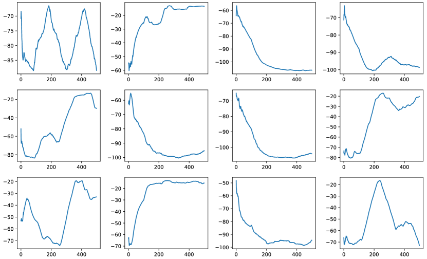
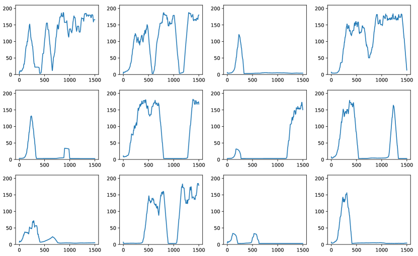
Attempts have also been made to improve the epoch efficiency of other hyperparameter optimization algorithms in [5, 7, 18] which predict the final learning outcome based on partially trained learning curves to identify hyperparameter settings that are expected to under-perform and early-stop them. In the context of DRL, however, these stopping criteria, including the exponential decay assumed in Freeze-thaw BO [42], may not be applicable, due to the unpredictable fluctuations of DRL reward curves. In the supplement, we illustrate the noisiness of DRL training.
The second category [16, 17, 23, 41, 48] aims to reduce the resource consumption of BO by utilizing low-fidelity functions which can be obtained by using a subset of the training data or by training the ML model for a small number of iterations. Multi-task BO [41] requires the user to define a division of the dataset into pre-defined and discrete subtasks. Multi-fidelity BO with continuous approximation (BOCA) [16] and hierarchical partition [34] extend this idea to continuous settings. Specifically, BOCA first selects the hyperparameter input and then the corresponding fidelity to be evaluated at. The fidelity in this context refers to the use of different number of learning iterations. Analogous to BOCA’s consideration of continuous fidelities, Fabolas [17] proposes to model the combined space of input hyperparameter and dataset size and then select the optimal input and dataset size jointly.
The above approaches typically identify performance of hyperparameters via the average (either training or validation) loss of the last learning iterations. Thereby, they do not account for potential noise in the learning process (e.g., they might select unstable settings that jumped to high performance in the last couple of iterations).
3 Bayesian Optimization for Iterative Learning (BOIL)
Problem setting.
We consider training a machine learning algorithm given a -dimensional hyperparameter for iterations. This process has a training time cost and produces training evaluations for iterations, . These could be episode rewards in DRL or training accuracies in DL. An important property of iterative training is that we know the whole curve at preceding steps .
Given the raw training curve , we assume an underlying smoothed black-box function , defined in Sec. 3.2. Formally, we aim to find ; at the same time, we want to keep the overall training time, , of evaluated settings as low as possible. We summarize our variables in Table in the supplement for ease of reading.
3.1 Selecting a next point using iteration-efficient modeling
We follow popular designs in [17, 19, 39, 41] and model the cost-sensitive black-box function as , where is an appropriate covariance functions and . For simplicity and robustness, the cost function is approximated by a linear regressor. Depending on the setting, it may be more appropriate to employ a second GP or different parametric model if the cost has a more complex dependence on hyperparameters and iterations . We regularly (re-)optimize both kernel and cost function parameters in between point acquisitions.
More specifically, we choose the covariance function as a product to induce joint similarities over parameter and iteration space. We estimate the predictive mean and uncertainty for a GP [31] at any input as
| (1) |
| (2) |
where , , , , and is the noise variance of . Cost predictions at any particular parameter and time are given by , where is directly computed from data as [1].
Our goal is to select a point with high function value (exploitation), high uncertainty (exploration) and low cost (cheap). At each iteration , we query the input parameter and the number of iteration [38, 48]:
| (3) |
Although our framework is available for any acquisition choices [13, 22, 47], to cope with output noise, we follow [45] and slight modify the expected improvement criterion using the maximum mean GP prediction . Let , we then have a closed-form for the new expected improvement (EI) as where is the standard normal p.d.f., is the c.d.f, and are the GP predictive mean and variance defined in Eq. (1) and Eq. (2), respectively.
3.2 Training curve compression and estimating the transformation function
Existing BO approaches [4, 23] typically define the objective function as an average loss over the final learning episodes. However, this does not take into consideration how stable performance is or the training stage at which it has been achieved. We argue that averaging learning losses is likely misleading due to the noise and fluctuations of our observations (learning curves) – particularly during the early stages of training. We propose to compress the whole learning curve into a numeric score via a preference function representing the user’s desired training curve. In the following, we use the Sigmoid function (specifically the Logistic function) to compute the utility score as
| (4) |
where is a dot product, a Logistic function is parameterized by a growth parameter defining a slope and the middle point of the curve . The optimal parameters and are estimated directly from the data. We illustrate different shapes of parameterized by and in the appendix. The Sigmoid preference has a number of desirable properties. As early weights are small, less credit is given to fluctuations at the initial stages, making it less likely for our surrogate to be biased towards randomly well performing settings. However, as weights monotonically increase, hyperparameters with improving performance are preferred. As weights saturate over time, stable, high performing configurations are preferred over short “performance spikes” characteristic of unstable training. Lastly, this utility score assigns higher values to the same performance if it is being maintained over more episodes.
Learning the transformation function from data.
Different compression curves , parameterized by different choices of and in Eq. (4), may lead to different utilities and thus affect the performance. The optimal values of and are unknown in advance. Therefore, we propose to learn these values and directly from the data. Our intuition is that the ‘optimal’ compression curve will lead to a better fit of the GP. This better GP surrogate model, thus, will result in better prediction as well as optimization performance. We parameterize the GP log marginal likelihood [31] as the function of and :
| (5) |
where is the output noise variance, is the function of and defined in Eq. (4). We optimize and (jointly with other GP hyperparameters) using multi-start gradient descent. We derive the derivative and which can be computed analytically as:
3.3 Augmenting the training data
When evaluating a parameter over iterations, we obtain not only a final score but also all reward sequences . The auxiliary information from the curve can be useful for BO. Therefore, we propose to augment the information from the curve into the sample set of our GP model.
A naïve approach for augmentation is to add a full curve of points where is computed using Eq. (4). However, this approach can be redundant and may impose serious issues in the conditioning of the GP covariance matrix. As we cluster more evaluations closely, the conditioning of the GP covariance degrades further, as discussed in [24]. This conditioning issue is especially serious in our noisy DRL settings.
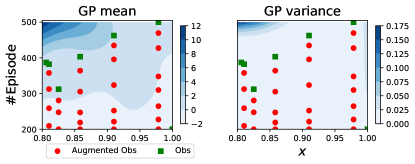
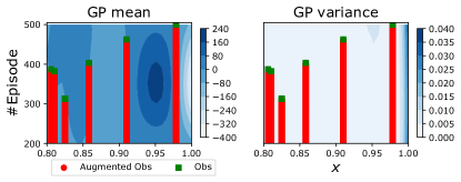
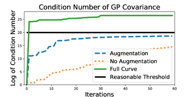
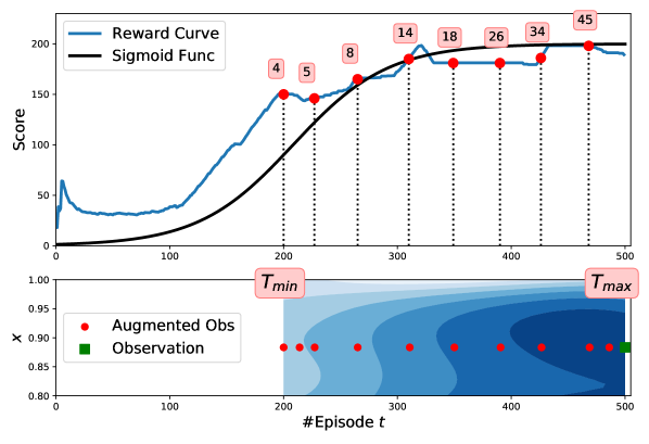
We highlight this effect on GP estimation in Fig. 2 wherein the GP mean varies erratically when the natural log of the condition number of the GP covariance matrix goes above (see Fig. 3) as we include the whole curve.
Selecting subset of points from the curve.
Different solutions, such as the addition of artificial noise or altering the kernel’s length-scales, have been proposed. We decide to use an active learning approach [10, 29] as sampled data points are expected to contain a lot of redundant information. As a consequence, the loss of information from sub-sampling the data should be minimal and information-eroding modification of the kernel matrix itself can be avoided. As a side benefit, the reduced number of sampled points speeds up inference in our GP models.
In particular, we select samples at the maximum of the GP predictive uncertainty. Formally, we sequentially select a set , , by varying while keeping fixed as
| (6) |
where . This sub-optimisation problem is done in a one-dimensional space of , thus it is cheap to optimize using (multi-start) gradient descent (the derivative of GP predictive variance is available [31]). Alternatively, a fixed-size grid could be considered, but this could cause conditioning issues when a point in the grid is placed near another existing point , i.e., for some small .
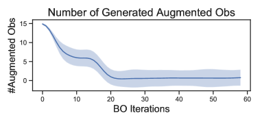
These generated points are used to calculate the output and augmented into the observation set for fitting the GP. The number of samples is adaptively chosen such that the natural log of the condition number of the covariance matrix is less than a threshold. This is to ensure that the GP covariance matrix condition number behaves well by reducing the number of unnecessary points added to the GP at later stages. We compute the utility score given for each augmented point using Eq. (4). In addition, we can estimate the running time using the predictive mean . We illustrate the augmented observations and estimated scores in Fig. 1.
We summarize the overall algorithm in Alg. 1. To enforce non-negativity and numerical stability, we make use of the transformations and .
4 Experiments
We assess our model by tuning hyperparameters for two DRL agents on three environments and a CNN on two datasets. We provide additional illustrations and experiments in the appendix.
Experimental setup.
All experimental results are averaged over independent runs with different random seeds. Final performance is estimated by evaluating the chosen hyperparameter over the maximum number of iterations. All experiments are executed on a NVIDIA 1080 GTX GPU using the tensorflow-gpu Python package. The DRL environments are available through the OpenAI gym [3] and Mujoco [43]. Our DRL implementations are based on the open source from Open AI Baselines [6]. We release our implementation at https://github.com/ntienvu/BOIL.
We use square-exponential kernels for the GP in our model and estimate their parameters by maximizing the marginal likelihood [31]. We set the maximum number of augmented points to be and a threshold for a natural log of GP condition number . We note that the optimization overhead is much less than the black-box function evaluation time.
Baselines.
We compare with Hyperband [23] which demonstrated empirical successes in tuning deep learning applications in an iteration-efficient manner. We extend the discrete multi-task BO [41] to the continuous case – which can also be seen as continuous multi-fidelity BO [16, 39] as in our setting, they both consider cost-sensitivity and iteration-efficiency. We, therefore, label the two baselines as continuous multi-task/fidelity BO (CM-T/F-BO). We have ignored the minor difference in these settings, such as multi-task approaches jointly optimizes the fidelity and input while BOCA [16] first selects the input and then the fidelity.
Our focus is to demonstrate the effectiveness of optimizing the learning curve using compression and augmentation techniques. We therefore omit the comparison of various acquisition functions and kernel choices which can easily be used in our model. We also do not compare with Fabolas [17] which is designed to vary dataset sizes, not iteration numbers. We would expect the performance of Fabolas to be close to CM-T/F-BO. We are unable to compare with FreezeThaw as the code is not available. However, the curves in our setting are not exponential decays and thus ill-suited to their model (see last figure in the appendix). We have considered an ablation study in the appendix using a time kernel following the exponential decay proposed in Freeze-thaw method [42].
Task descriptions.
We consider three DRL settings including a Dueling DQN (DDQN) [46] agent in the CartPole-v0 environment and Advantage Actor Critic (A2C) [25] agents in the InvertedPendulum-v2 and Reacher-v2 environments. In addition to the DRL applications, we tune hyperparameters for training a convolutional neural network [21] on the SVHN dataset and CIFAR10. Due to space considerations, we refer to the appendix for further details.
4.1 Model illustration
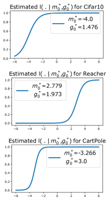
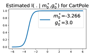
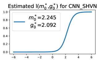
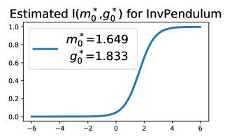
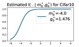
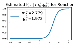
We first illustrate the estimated compression function in Right Fig. 1 from different experiments. These Logistic parameters and are estimated by maximizing the GP marginal likelihood and used for compressing the curve. We show that the estimated curve from CartPole tends to reach the highest performance much earlier than Reacher because CartPole is somewhat easier to train than Reacher.
We next examine the count of augmented observations generated per iteration in Fig. 4. Although this number is fluctuating, it tends to reduce over time. BOIL does not add more augmented observations at the later stage when we have gained sufficient information and GP covariance conditioning falls below our threshold .
4.2 Ablation study of curve compression
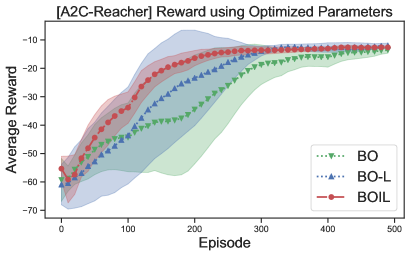
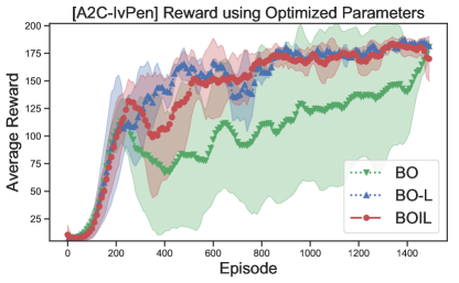
To demonstrate the impact of our training curve compression, we compare BOIL to vanilla Bayesian optimization (BO) and with compression (BO-L) given the same number of iterations at . We show that using the curve compression leads to stable performance, as opposed to the existing technique of averaging the last iterations. We plot the learning curves of the best hyperparameters identified by BO, BO-L and BOIL. Fig. 5 shows the learning progress over episodes for each of these. The curves are smoothed by averaging over consecutive episodes for increased clarity. We first note that all three algorithms eventually obtain similar performance at the end of learning. However, since BO-L and BOIL take into account the preceding learning steps, they achieve higher performance more quickly. Furthermore, they achieve this more reliably as evidenced by the smaller error bars (shaded regions).
4.3 Tuning deep reinforcement learning and CNN
We now optimize hyperparameters for deep reinforcement learning algorithms; in fact, this application motivated the development of BOIL. The combinations of hyperparameters to be tuned, target DRL algorithm and environment can be found in the appendix.
Comparisons by iterations and real-time.
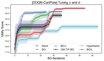
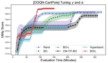
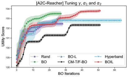
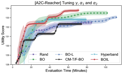
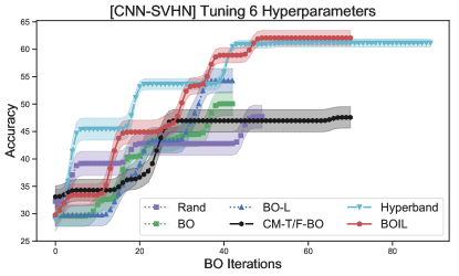
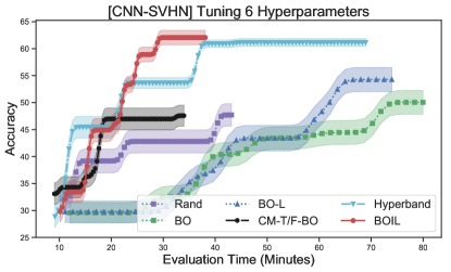
Fig. 6 illustrates the performance of different algorithms against the number of iterations as well as real-time (the plots for CIFAR10 are in the appendix). The performance is the utility score of the best hyperparameters identified by the baselines. Across all three tasks, BOIL identifies optimal hyperparameters using significantly less computation time than other approaches.
The plots show that other approaches such as BO and BO-L can identify well-performing hyperparameters in fewer iterations than BOIL. However, they do so only considering costly, high-fidelity evaluations resulting in significantly higher evaluation times. In contrast to this behavior, BOIL accounts for the evaluation costs and chooses to initially evaluate low-fidelity settings consuming less time. This allows fast assessments of a multitude of hyperparameters. The information gathered here is then used to inform later point acquisitions. Hereby, the inclusion of augmented observations is crucial in offering useful information readily available from the data. In addition, this augmentation is essential to prevent from the GP kernel issue instead of adding the full curve of points into our GP model.
Hyperband [23] exhibits similar behavior in that it uses low fidelity (small ) evaluations to reduce a pool of randomly sampled configurations before evaluating at high fidelity (large ). To deal with noisy evaluations and other effects, this process is repeated several times. This puts Hyperband at a disadvantage particularly in the noisy DRL tasks. Since early performance fluctuates hugely, Hyperband can be misled in where to allocate evaluation effort. It is then incapable of revising these choices until an entirely new pool of hyperparameters is sampled and evaluated from scratch. In contrast to this, BOIL is more flexible than Hyperband in that it can freely explore-exploit the whole joint space. The GP surrogate hereby allows BOIL to generalize across hyperparameters and propagate information through the joint space.
5 Conclusion and Future work
Our framework complements the existing BO toolbox for hyperparameter tuning with iterative learning. We present a way of leveraging our understanding that later stages of the training process are informed by progress made in earlier ones. This results in a more iteration-efficient hyperparameter tuning algorithm that is applicable to a broad range of machine learning systems. We evaluate its performance on a set of diverse benchmarks. The results demonstrate that our model surpasses the performance of well-established alternatives while consuming significantly fewer resources. Finally, we note that our approach is not necessarily specific to machine learning algorithms, but more generally applies to any process exhibiting an iterative structure to be exploited.
6 Broader Impact
Our work aims at making the optimization of processes operating in a step-wise fashion more efficient. As demonstrated this makes BOIL particularly well-suited to supporting supervised learning models and RL systems. By increasing training efficience of these models, we hope to contribute to their widespread deployment whilst reducing the computational and therefore environmental cost their implementation has.
Deep (reinforcement) learning systems find application in a wide range of settings that directly contribute to real world decisions, e.g., natural language processing, visual task, autonomous driving and many more. As machine learning models building on our contributions are being deployed in the real world, we encourage practicioners to put in place necessary supervision and override mechanisms as precautions against potential failure.
In a more general context, our algorithm may be seen as a step towards the construction of an automated pipeline for the training and deployment of machine learning models. A potential danger is that humans become further and further removed from the modelling process, making it harder to spot (potentially critical) failures. We do not see this as an argument against the construction of such a pipeline in principle, but instead encourage practicioners to reflect on potential biases indirectly encoded in the choice of data sets and models, they are feeding into said automated processes.
The growing opacity of machine learning models is a concern of its own and which automated training procedures will only contribute to. Opposing this is a rapidly growing corpus of work addressing the interpretability of trained machine learning models and their decision making. These can and should be used to rigorously analyse final training outcomes. Only then can we ensure that machine learning algorithm do indeed become a beneficial source of information guiding real world policy making as opposed to opaque, unquestioned entities.
While our main interest lies in the hyperparameter optimization of machine learning models, it should be noted that any iterative process depending on a set of parameters can make use of our contributions. Possible settings could, for instance, include the optimization of manufacturing pipelines in which factory setting are adjusted to increase productivity.
7 Acknowledgements
S. Schulze is supported by an I-CASE studentship funded by the EPSRC and Dyson.
References
- [1] Christopher M Bishop. Pattern recognition and machine learning. springer New York, 2006.
- [2] Eric Brochu, Vlad M Cora, and Nando De Freitas. A tutorial on Bayesian optimization of expensive cost functions, with application to active user modeling and hierarchical reinforcement learning. arXiv preprint arXiv:1012.2599, 2010.
- [3] Greg Brockman, Vicki Cheung, Ludwig Pettersson, Jonas Schneider, John Schulman, Jie Tang, and Wojciech Zaremba. Openai gym. arXiv preprint arXiv:1606.01540, 2016.
- [4] Yutian Chen, Aja Huang, Ziyu Wang, Ioannis Antonoglou, Julian Schrittwieser, David Silver, and Nando de Freitas. Bayesian optimization in AlphaGo. arXiv preprint arXiv:1812.06855, 2018.
- [5] Zhongxiang Dai, Haibin Yu, Bryan Kian Hsiang Low, and Patrick Jaillet. Bayesian optimization meets Bayesian optimal stopping. In International Conference on Machine Learning, pages 1496–1506, 2019.
- [6] Prafulla Dhariwal, Christopher Hesse, Oleg Klimov, Alex Nichol, Matthias Plappert, Alec Radford, John Schulman, Szymon Sidor, Yuhuai Wu, and Peter Zhokhov. Openai baselines. GitHub, GitHub repository, 2017.
- [7] Tobias Domhan, Jost Tobias Springenberg, and Frank Hutter. Speeding up automatic hyperparameter optimization of deep neural networks by extrapolation of learning curves. In Twenty-Fourth International Joint Conference on Artificial Intelligence, 2015.
- [8] Stefan Falkner, Aaron Klein, and Frank Hutter. Bohb: Robust and efficient hyperparameter optimization at scale. In International Conference on Machine Learning, pages 1436–1445, 2018.
- [9] Peter I Frazier. A tutorial on Bayesian optimization. arXiv preprint arXiv:1807.02811, 2018.
- [10] Yarin Gal, Riashat Islam, and Zoubin Ghahramani. Deep Bayesian active learning with image data. In Proceedings of the 34th International Conference on Machine Learning, pages 1183–1192, 2017.
- [11] Peter Henderson, Riashat Islam, Philip Bachman, Joelle Pineau, Doina Precup, and David Meger. Deep reinforcement learning that matters. In Thirty-Second AAAI Conference on Artificial Intelligence, 2018.
- [12] Philipp Hennig and Christian J Schuler. Entropy search for information-efficient global optimization. Journal of Machine Learning Research, 13:1809–1837, 2012.
- [13] José Miguel Hernández-Lobato, Matthew W Hoffman, and Zoubin Ghahramani. Predictive entropy search for efficient global optimization of black-box functions. In Advances in Neural Information Processing Systems, pages 918–926, 2014.
- [14] Donald R Jones, Matthias Schonlau, and William J Welch. Efficient global optimization of expensive black-box functions. Journal of Global optimization, 13(4):455–492, 1998.
- [15] M. I. Jordan and T. M. Mitchell. Machine learning: Trends, perspectives, and prospects. Science, 349(6245):255–260, 2015.
- [16] Kirthevasan Kandasamy, Gautam Dasarathy, Jeff Schneider, and Barnabás Póczos. Multi-fidelity Bayesian optimisation with continuous approximations. In Proceedings of the 34th International Conference on Machine Learning, pages 1799–1808, 2017.
- [17] Aaron Klein, Stefan Falkner, Simon Bartels, Philipp Hennig, and Frank Hutter. Fast Bayesian optimization of machine learning hyperparameters on large datasets. In Artificial Intelligence and Statistics, pages 528–536, 2017.
- [18] Aaron Klein, Stefan Falkner, Jost Tobias Springenberg, and Frank Hutter. Learning curve prediction with Bayesian neural networks. International Conference on Learning Representations (ICLR), 2017.
- [19] Andreas Krause and Cheng S Ong. Contextual Gaussian process bandit optimization. In Advances in Neural Information Processing Systems, pages 2447–2455, 2011.
- [20] Alex Krizhevsky, Ilya Sutskever, and Geoffrey E Hinton. Imagenet classification with deep convolutional neural networks. In Advances in Neural Information Processing Systems, pages 1097–1105, 2012.
- [21] Yann LeCun, Léon Bottou, Yoshua Bengio, and Patrick Haffner. Gradient-based learning applied to document recognition. Proceedings of the IEEE, 86(11):2278–2324, 1998.
- [22] Benjamin Letham, Brian Karrer, Guilherme Ottoni, Eytan Bakshy, et al. Constrained Bayesian optimization with noisy experiments. Bayesian Analysis, 14(2):495–519, 2019.
- [23] Lisha Li and Kevin Jamieson. Hyperband: A novel bandit-based approach to hyperparameter optimization. Journal of Machine Learning Research, 18:1–52, 2018.
- [24] Mark McLeod, Stephen Roberts, and Michael A Osborne. Optimization, fast and slow: Optimally switching between local and Bayesian optimization. In International Conference on Machine Learning, pages 3440–3449, 2018.
- [25] Volodymyr Mnih, Adria Puigdomenech Badia, Mehdi Mirza, Alex Graves, Timothy Lillicrap, Tim Harley, David Silver, and Koray Kavukcuoglu. Asynchronous methods for deep reinforcement learning. In International conference on machine learning, pages 1928–1937, 2016.
- [26] Volodymyr Mnih, Koray Kavukcuoglu, David Silver, Alex Graves, Ioannis Antonoglou, Daan Wierstra, and Martin Riedmiller. Playing atari with deep reinforcement learning. NIPS Deep Learning Workshop, 2013.
- [27] Vu Nguyen, Sunil Gupta, Santu Rana, Cheng Li, and Svetha Venkatesh. Regret for expected improvement over the best-observed value and stopping condition. In Proceedings of The 9th Asian Conference on Machine Learning (ACML), pages 279–294, 2017.
- [28] Vu Nguyen and Michael A Osborne. Knowing the what but not the where in Bayesian optimization. In International Conference on Machine Learning, pages 7317–7326, 2020.
- [29] Michael Osborne, Roman Garnett, Zoubin Ghahramani, David K Duvenaud, Stephen J Roberts, and Carl E Rasmussen. Active learning of model evidence using Bayesian quadrature. In Advances in Neural Information Processing Systems, pages 46–54, 2012.
- [30] Jack Parker-Holder, Vu Nguyen, and Stephen Roberts. Provably efficient online hyperparameter optimization with population-based bandits. In Advances in Neural Information Processing Systems, 2020.
- [31] Carl Edward Rasmussen. Gaussian processes for machine learning. 2006.
- [32] Binxin Ru, Mark McLeod, Diego Granziol, and Michael A Osborne. Fast information-theoretic Bayesian optimisation. In International Conference on Machine Learning, pages 4381–4389, 2018.
- [33] Tom Schaul, John Quan, Ioannis Antonoglou, and David Silver. Prioritized experience replay. International Conference on Learning Representations, 2016.
- [34] Rajat Sen, Kirthevasan Kandasamy, and Sanjay Shakkottai. Multi-fidelity black-box optimization with hierarchical partitions. In International conference on machine learning, pages 4538–4547, 2018.
- [35] Bobak Shahriari, Kevin Swersky, Ziyu Wang, Ryan P Adams, and Nando de Freitas. Taking the human out of the loop: A review of Bayesian optimization. Proceedings of the IEEE, 104(1):148–175, 2016.
- [36] David Silver, Aja Huang, Chris J Maddison, Arthur Guez, Laurent Sifre, George Van Den Driessche, Julian Schrittwieser, Ioannis Antonoglou, Veda Panneershelvam, Marc Lanctot, et al. Mastering the game of go with deep neural networks and tree search. Nature, 529(7587):484, 2016.
- [37] Leslie N Smith. A disciplined approach to neural network hyper-parameters: Part 1–learning rate, batch size, momentum, and weight decay. arXiv preprint arXiv:1803.09820, 2018.
- [38] Jasper Snoek, Hugo Larochelle, and Ryan P Adams. Practical Bayesian optimization of machine learning algorithms. In Advances in Neural Information Processing Systems, pages 2951–2959, 2012.
- [39] Jialin Song, Yuxin Chen, and Yisong Yue. A general framework for multi-fidelity Bayesian optimization with Gaussian processes. In The 22nd International Conference on Artificial Intelligence and Statistics, pages 3158–3167, 2019.
- [40] Niranjan Srinivas, Andreas Krause, Sham Kakade, and Matthias Seeger. Gaussian process optimization in the bandit setting: No regret and experimental design. In Proceedings of the 27th International Conference on Machine Learning, pages 1015–1022, 2010.
- [41] Kevin Swersky, Jasper Snoek, and Ryan P Adams. Multi-task Bayesian optimization. In Advances in Neural Information Processing Systems, pages 2004–2012, 2013.
- [42] Kevin Swersky, Jasper Snoek, and Ryan Prescott Adams. Freeze-thaw Bayesian optimization. arXiv preprint arXiv:1406.3896, 2014.
- [43] Emanuel Todorov, Tom Erez, and Yuval Tassa. Mujoco: A physics engine for model-based control. In 2012 IEEE/RSJ International Conference on Intelligent Robots and Systems, pages 5026–5033. IEEE, 2012.
- [44] Zi Wang and Stefanie Jegelka. Max-value entropy search for efficient Bayesian optimization. In International Conference on Machine Learning, pages 3627–3635, 2017.
- [45] Ziyu Wang and Nando de Freitas. Theoretical analysis of Bayesian optimisation with unknown Gaussian process hyper-parameters. arXiv preprint arXiv:1406.7758, 2014.
- [46] Ziyu Wang, Tom Schaul, Matteo Hessel, Hado Hasselt, Marc Lanctot, and Nando Freitas. Dueling network architectures for deep reinforcement learning. In International Conference on Machine Learning, pages 1995–2003, 2016.
- [47] Jian Wu and Peter Frazier. The parallel knowledge gradient method for batch Bayesian optimization. In Advances In Neural Information Processing Systems, pages 3126–3134, 2016.
- [48] Jian Wu, Saul Toscano-Palmerin, Peter I Frazier, and Andrew Gordon Wilson. Practical multi-fidelity Bayesian optimization for hyperparameter tuning. In 35th Conference on Uncertainty in Artificial Intelligence, 2019.
The following sections are intended to give the reader further insights into our design choices and a deeper understanding of the algorithms properties. First, we give a brief overview of Bayesian optimization with Gaussian processes. We then illustrate our models behavior on a two dimensional problem. Last, we give further details of our experiments for reproducibility purposes.
Appendix A Bayesian Optimization Preliminaries
Bayesian optimization is a sequential approach to global optimization of black-box functions without making use of derivatives. It uses two components: a learned surrogate model of the objective function and an acquisition function derived from the surrogate for selecting new points to inform the surrogate with. In-depth discussions beyond our brief overview can be found in recent surveys [2, 9, 35].
Notation.
We summarize all of the notations used in our model in Table 1 for ease of reading.
A.1 Gaussian processes
We present the GP surrogate model for the black-box function [31]. A GP defines a probability distribution over functions under the assumption that any subset of points is normally distributed. Formally, this is denoted as:
where and are the mean and covariance functions, given by and .
Typically, the mean of the GP is assumed to be zero everywhere. The kernel can be thought of as a similarity measure relating and . Numerous kernels encoding different prior beliefs about have been proposed. A popular choice is given by the square exponential kernel . The length- and output-scales and regulate the maximal covariance between two points and can be estimated using maximum marginal likelihood. The SE kernel encodes the belief that nearby points are highly correlated as it is maximized at and decays the further and are separated.
For predicting at a new data point , assuming a zero mean , we have:
| (11) |
where , and . The conditional probability of follows a univariate Gaussian distribution as . Its mean and variance are given by:
As GPs give full uncertainty information with any prediction, they provide a flexible nonparametric prior for Bayesian optimization. We refer the interested readers to [31] for further details on GPs.
| Parameter | Domain | Meaning |
|---|---|---|
| integer, | dimension, no. of hyperparameters to be optimized | |
| vector, | input hyperparameter | |
| integer, | maximum number of BO iterations | |
| , | integer, | the min/max no of iterations for training a ML algorithm |
| index of training steps | ||
| integer, | the maximum number of augmentation. We set . | |
| scalar, | threshold for rejecting augmentation when ln of cond | |
| index of augmenting variables | ||
| index of BO iterations | ||
| vector, | concatenation of the parameter and iteration | |
| scalar, | training cost (sec) | |
| scalar, | transformed score at the BO iteration | |
| scalar, | transformed score at the BO iteration , training step | |
| function | acquisition function for performance | |
| function | estimation of the cost by LR given and | |
| function | a raw learning curve, | |
| function | a black-box function which is compressed from the above | |
| function | Logistic curve | |
| , | scalar, | a growth parameter defining a slope, |
| , | scalar, | a middle point parameter, |
| scalar, | Gaussian process log marginal likelihood |
A.2 Acquisition function
Bayesian optimization is typically applied in settings in which the objective function is expensive to evaluate. To minimize interactions with that objective, an acquisition function is defined to reason about the selection of the next evaluation point . The acquisition function is constructed from the predictive mean and variance of the surrogate to be easy to evaluate and represents the trade-off between exploration (of points with high predictive uncertainty) and exploitation (of points with high predictive mean). Thus, by design the acquisition function can be maximized with standard global optimization toolboxes. Among the many acquisition functions [12, 13, 14, 32, 40, 44] available in the literature, the expected improvement [14, 27, 45] is one of the most popular.
A.3 GP kernels and treatment of GP hyperparameters
We present the GP kernels and treatment of GP hyperparameters for the black-box function .
Although the raw learning curve in DRL is noisy, the transformed version using our proposed curve compression is smooth. Therefore, we use two squared exponential kernels for input hyperparameter and training iteration, respectively. That is and where the observation and are normalized to and the outcome is standardized for robustness. As a result, our product kernel becomes
The length-scales and are learnable parameters indicating the variability of the function with regards to the hyperparameter input and number of training iterations . Estimating appropriate values for them is critical as this represents the GPs prior regarding the sensitivity of performance w.r.t. changes in the number of training iterations and hyperparameters. For extremely large we expect the objective function to change very little for different numbers of training iterations. For small by contrast we expect drastic changes even for small differences. We estimate these GP hyperparameters (including the length-scales , and the output noise variance ) by maximizing their log marginal likelihood [31].
We optimize Eq. (5) with a gradient-based optimizer, providing the analytical gradient to the algorithm. We start the optimization from the previous hyperparameter values . If the optimization fails due to numerical issues, we keep the previous value of the hyperparameters. We refit the hyperparameters every function evaluations where is the dimension.


Appendix B Algorithm Illustration and Further Experiments
| Variables | Min | Max | Best Found |
|---|---|---|---|
| discount factor | |||
| learning rate model | |||
| #Episodes | - |
Fig. 7 and Fig. 8 illustrate the behavior of our proposed algorithm BOIL on the example of optimizing the discount factor of Dueling DQN [46] on the CartPole problem. The two settings differ in the inclusion augmented observations into BOIL in Fig. 7 and CM-T/F-BO (or BOIL without augmented observations) in Fig. 8.
In both cases, we plot the GP predictive mean in Eq. (1), GP predictive variance in Eq. (2), the acquisition function in Eq. (3), the predicted function and the final decision function in Eq. (8). These equations are defined in the main manuscript.
| Variables | Min | Max | Best Found |
|---|---|---|---|
| discount factor | |||
| learning rate actor | |||
| learning rate critic | |||
| #Episodes | - |
| Min | Max | Best Found | |
|---|---|---|---|
| - |
As shown in the respective figures the final decision function balances between utility and cost of any pair to achieve iteration efficiency. Especially in situations where multiple locations share the same utility value, our decision will prefer to select the cheapest option. Using the augmented observations in Fig. 7, our joint space is filled quicker with points and the uncertainty (GP variance) across it reduces faster than in Fig. 8 – the case of vanilla CM-T/F-BO without augmenting observations. A second advantage of having augmented observations is that the algorithm is discouraged to select the same hyperparameter setting at lower fidelity than a previous evaluation. We do not add the full curve as it can be redundant while causing the conditioning problem of the GP covariance matrix.
B.1 Experiment settings
We summarize the hyperparameter search ranges for A2C on Reacher and InvertedPendulum in Table 3, CNN on SHVN in Table 4 and DDQN on CartPole in Table 2. Additionally, we present the best found parameter for these problems. Further details of the DRL agents are listed in Table 5.
| Variables | Min | Max | Best Found |
|---|---|---|---|
| filter size | |||
| pool size | |||
| batch size | |||
| learning rate | |||
| momentum | |||
| decay | |||
| number of epoch | - |
| Hyperparameter | Value |
|---|---|
| A2C | |
| Critic-network architecture | |
| Actor-network architecture | |
| Entropy coefficient | |
| Dueling DQN | |
|---|---|
| Q-network architecture | |
| ε-greedy (start, final, number of steps) | |
| Buffer size | |
| Batch size | |
| PER- [33] | |
| PER- (start, final, number of steps) | |
B.2 Learning Logistic Function
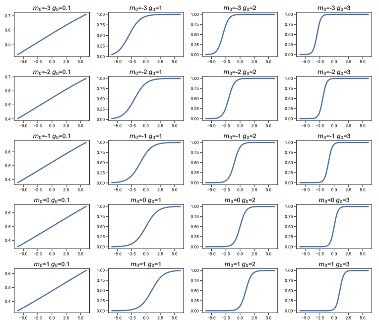
We first present the Logistic curve using different choices of and in Fig. 10. We then learn from the data to get the optimal choices and presented in Fig. 11.
B.3 Robustness over Different Preference Functions
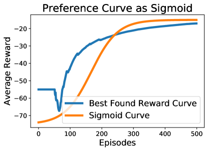
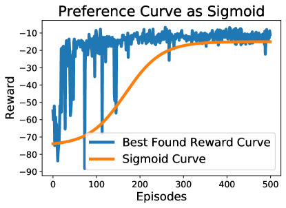
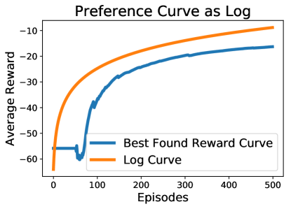
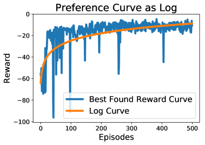
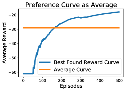
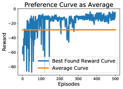
We next study the learning effects with respect to different choices of the preference functions. We pick three preference functions including the Sigmoid, Log and Average to compute the utility score for each learning curve. Then, we report the best found reward curve under such choices. The experiments are tested using A2C on Reacher-v2. The results presented in Fig. 9 demonstrate the robustness of our model with the preference functions.
B.4 Applying Freeze-Thaw BO in the settings considered
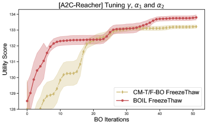
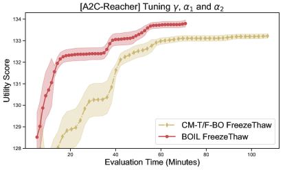
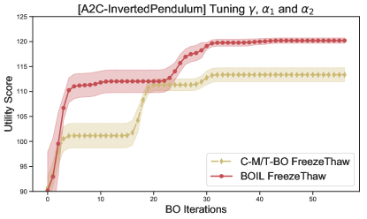
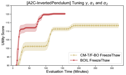
While both the exponential decay in Freeze-Thaw BO [42] and our compression function encode preferences regarding training development, there is an important distinction between the two approaches. Freeze-thaw BO utilises the exponential decay property to terminate the training curve, while BOIL only uses the sigmoid curve to guide the search. We refer to Fig. 13 for further illustration of why Freeze-thaw BO struggles in DRL settings.

B.5 Ablation Study using Freeze-Thraw Kernel for Time
In the joint modeling framework of hyperparameter and time (iteration), we can replace the kernel either or with different choices. We, therefore, set up a new baseline of using the time-kernel in Freeze-Thaw approach [42] which encodes the monotonously exponential decay from the curve. Particularly, we use the kernel defined as
for parameters which are optimized in the GP models.
We present the result in Fig. 14 that CM-T/F-BO is still less competitive to BOIL using this specific time kernel. The results again validate the robustness our approach cross different choices of kernel.
B.6 Additional Experiments for Tuning DRL and CNN
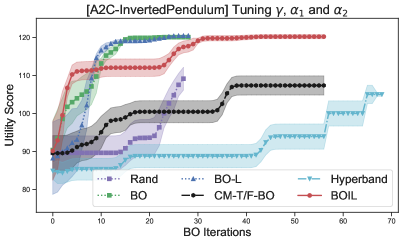
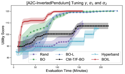
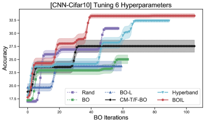
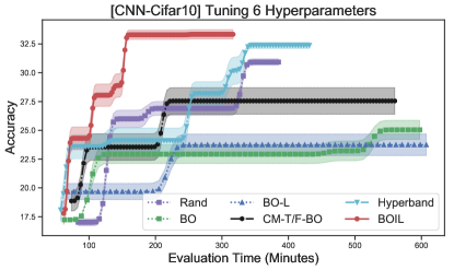
We present the additional experiments for tuning a DRL model using InvertedPendulum environment and a CNN model using a subset of CIFAR10 in Fig. 12. Again, we show that the proposed model clearly gain advantages against the baselines in tuning hyperparameters for model with iterative learning information available.
B.7 Examples of Deep Reinforcement Learning Training Curves
Finally, we present examples of training curves produced by the deep reinforcement learning algorithm A2C in Fig. 15. These fluctuate widely and it may not be trivial to define good stopping criteria as done for other applications in previous work [42].
