An inexact proximal augmented Lagrangian framework with arbitrary linearly convergent inner solver for composite convex optimization

Abstract

We propose an inexact proximal augmented Lagrangian framework with explicit inner problem termination rule for composite convex optimization problems. We consider arbitrary linearly convergent inner solver including in particular stochastic algorithms, making the resulting framework more scalable facing the ever-increasing problem dimension. Each subproblem is solved inexactly with an explicit and self-adaptive stopping criterion, without requiring to set an a priori target accuracy. When the primal and dual domain are bounded, our method achieves $O(1/\sqrt{\epsilon})$ and $O(1/{\epsilon})$ complexity bound in terms of number of inner solver iterations, respectively for the strongly convex and non-strongly convex case. Without the boundedness assumption, only logarithm terms need to be added and the above two complexity bounds increase respectively to $\tilde{O}(1/\sqrt{\epsilon})$ and $\tilde{O}(1/{\epsilon})$, which hold both for obtaining $\epsilon$-optimal and $\epsilon$-KKT solution. Within the general framework that we propose, we also obtain $\tilde{O}(1/{\epsilon})$ and $\tilde{O}(1/{\epsilon^{2}})$ complexity bounds under relative smoothness assumption on the differentiable component of the objective function. We show through theoretical analysis as well as numerical experiments the computational speedup possibly achieved by the use of randomized inner solvers for large-scale problems.

1 Introduction

We consider the following optimization problem:

$$\min_{x\in\mathbb{R}^{n}}~{}~{} f(x)+g(x)+h_{1}(p_{1}(x))+h_{2}(p_{2}(x)).$$ (1)

Here $g:\mathbb{R}^{n}\rightarrow\mathbb{R}\cup\{+\infty\}$, $h_{1}:\mathbb{R}^{d_{1}}\rightarrow\mathbb{R}$ are proper, convex and closed functions. The function $h_{2}:\mathbb{R}^{d_{2}}\rightarrow\mathbb{R}\cup\{+\infty\}$ is the indicator function of a convex and closed set $\mathcal{K}\subset\mathbb{R}^{d_{2}}$:

$$h_{2}(u_{2})=\left\{\begin{array}[]{ll}0&\mathrm{if~{}}u_{2}\in\mathcal{K}\\ +\infty&\mathrm{otherwise}\end{array}\right.$$ (2)

The function $f:\mathbb{R}^{n}\rightarrow\mathbb{R}\cup\{+\infty\}$ is convex and differentiable on an open set containing $\operatorname{dom}(g)$. The functions $p_{1}:\mathbb{R}^{n}\rightarrow\mathbb{R}^{d_{1}}$ and $p_{2}:\mathbb{R}^{n}\rightarrow\mathbb{R}^{d_{2}}$ are differentiable. In addition, we assume that $g,h_{1},h_{2}$ are simple functions, in the sense that their proximal operator are easily computable. With some other standard assumptions stated in the later discussion, the model that we consider covers a wide range of optimization problems. As an example, the following linearly constrained convex optimization problem

$$\min_{x\in\mathbb{R}^{n}}~{}~{}~{}f(x)+g(x)$$ (3)

$$\enspace s.t.\qquad Ax=b$$

is a special case of (1) by letting $h_{1}\equiv 0$, $\mathcal{K}=\{b\}$ and $p_{2}(x)\equiv Ax$. Important applications of (3) include model predictive control [38] and basis pursuit problem [12]. When $h_{1}\equiv 0$, $\mathcal{K}$ is a closed convex cone in $\mathbb{R}^{d_{2}}$ and $p_{2}(\cdot)$ is convex with respect to $\mathcal{K}$, problem (1) reduces to the convex conic programming model [27, 25] and in particular contains the constrained convex programming problem [36]:

$$\min_{x\in\mathbb{R}^{n}}~{}~{}~{}f(x)+g(x)$$ (4)

$$\enspace s.t.\quad f_{1}(x)\leq 0,\enspace\cdots,f_{m}(x)\leq 0.$$

Apart from constrained programs, problem (1) also covers many popular models in machine learning, including the sparse-group LASSO [39], the fused LASSO [40], the square root LASSO [6], and the support vector machine problem [49].

In [36], Rockafellar built an inexact augmented Lagrangian method (ALM) framework for solving (4). At each iteration of the inexact ALM, one needs to solve a convex optimization problem (referred to as inner problem) presumed easier than the original constrained problem (4), up to a certain accuracy. Rockafellar [36] gave some stopping criteria for the test of the inner problem solution accuracy, as well as some sufficient conditions guaranteeing the convergence of the inexact ALM method. In [30], Nesterov proposed a smoothing technique to deal with the unconstrained case ($h_{2}\equiv 0$). The idea is again to replace the original problem by an easier subproblem and solve it up to a desired accuracy. Although existing work usually consider either $h_{1}\equiv 0$ or $h_{2}\equiv 0$ [7, 10], we can treat them in a unified way because the augmented Lagrangian function corresponds to a smooth approximation of the function $h_{2}$. In fact, both Rockafellar’s inexact ALM framework and Nesterov’s smoothing technique are applications of the inexact proximal point method [37, 5]. There is no essential difficulty in extending existing results from the case $h_{1}\equiv 0$ or $h_{2}\equiv 0$ to the general model (1). For this reason, in the following discussion, we do not make particular difference between the papers dealing with the two different cases (either $h_{1}\equiv 0$ or $h_{2}\equiv 0$).

We mainly consider two optimality criteria for the complexity analysis of inexact ALM. One is based on the primal feasibility and the primal value optimality gap and the other on the KKT-residual. A solution $x\in\operatorname{dom}(g)$ is said to be $\epsilon$-optimal if [36, 30, 5, 28, 33, 27, 46]

$$|F(x)-F^{\star}|\leq\epsilon,\enspace\operatorname{dist}(p_{2}(x),\mathcal{K})\leq\epsilon.$$ (5)

Here,

$$F(x):=f(x)+g(x)+h_{1}(p_{1}(x)),\enspace\forall x\in\mathbb{R}^{n},$$ (6)

and $F^{\star}$ denotes the optimal value of (1). A solution $x\in\operatorname{dom}(g)$ is said to be $\epsilon$-KKT optimal if there is $\lambda_{1}\in\operatorname{dom}(h_{1}^{*})$ and $\lambda_{2}\in\operatorname{dom}(h_{2}^{*})$ such that [21, 25]

$$\operatorname{dist}(0,\partial_{x}L(x,\lambda_{1},\lambda_{2}))\leq\epsilon,\enspace\operatorname{dist}(0,\partial_{\lambda_{1}}L(x,\lambda_{1},\lambda_{2}))\leq\epsilon,\enspace\operatorname{dist}(0,\partial_{\lambda_{2}}L(x,\lambda_{1},\lambda_{2}))\leq\epsilon.$$ (7)

Here,

$$L(x,\lambda_{1},\lambda_{2}):=f(x)+g(x)+\langle\lambda_{1},p_{1}(x)\rangle-h_{1}^{*}(\lambda_{1})+\langle\lambda_{2},p_{2}(x)\rangle-h_{2}^{*}(\lambda_{2}),\enspace\forall x\in\mathbb{R}^{n},\lambda_{1}\in\mathbb{R}^{d_{1}},\lambda_{2}\in\mathbb{R}^{d_{2}},$$

denotes the Lagrangian function. A different criterion which can be derived from (7) under the boundedness of $\operatorname{dom}(g)$ was used in [23]. Most of the previously cited papers studied the complexity bound of the inexact ALM, which is the number of inner iterations needed for computing an $\epsilon$-optimal solution or an $\epsilon$-KKT solution. The lowest known complexity bound is $O(\epsilon)$ for obtaining an $\epsilon$-optimal solution [30, 5, 33, 27, 46, 41], and $\tilde{O}(\epsilon)$ for obtaining an $\epsilon$-KKT solution [25].

There are some variants of inexact ALM which avoid the solution of inner problems, including the linearized ALM [46] and linearized ADMM [32] as well as their stochastic extensions [45, 47, 9]. These inner problem free methods are widely used in practice thanks to their simple implementation form and good practical convergence behavior. However, $O(\epsilon)$ complexity bound of these methods are established only in an ergodic sense, not in the last iterate. In [42], an accelerated smooth gap reduction method (ASGARD) was developed with a non-ergodic $O(\epsilon)$ complexity bound and showed superior numerical performance than linearized ADMM. The method has been extended to a stochastic block coordinate update version in [1], called SMART-CD. In practice, it was observed that appropriately restarting ASGARD or SMART-CD can further speed up the convergence. In [41], the authors analyzed a double-loop ASGARD (ASGARD-DL) which achieves the non-ergodic complexity bound $O(\epsilon)$ and has similar practical convergence behavior as ASGARD with restart. ASGARD-DL [41] can be seen as an inexact ALM. However, in contrast to a series of work on inexact ALM [30, 5, 33, 27, 46], ASGARD-DL has an explicit inner termination rule and does not require the boundedness of $\operatorname{dom}(g)$.

The boundedness assumption of $\operatorname{dom}(g)$ seems to be crucial in the existing analysis for inexact ALM since it allows to directly control the number of iterations needed for the solution of each inner problem, using deterministic first-order solvers such as the accelerated proximal gradient (APG) [4]. It was argued that such boundedness assumption is mild because in some cases it is possible to find a bounded set including the optimal solution [23]. Nevertheless, removing this assumption from the complexity analysis of inexact ALM seems to be challenging and requires different approaches from existing ones. ASGARD-DL [41] is among the first which achieve the best complexity bound $O(\epsilon)$ without making the compactness assumption. However, their analysis builds on a very special property of APG and thus excludes the possibility of other inner solvers.

Allowing more flexible choice of inner solver is a very important feature in the large-scale setting. It is recognized that some randomized first-order methods can be more efficient than APG when the problem dimension is high. This includes for example the randomized coordinate descent variant of APG (a.k.a. APPROX) [16] and the stochastic variance reduced variant of APG (a.k.a. Katyusha) [2]. Compared with their deterministic origin APG, APPROX can reduce the computation load when the number of coordinates $n$ is large, while Katyusha is more efficient when the number of constraints $m$ (in (4)) is large. With the ever-increasing scale of the problems to be solved, it is necessary to employ randomized methods for solving the inner problems. However, the complexity analysis of inexact ALM with randomized inner solvers seems not to have been fully investigated.

In this paper, we develop an inexact proximal ALM which does not require the boundedness of $\operatorname{dom}(g)$ for the inner termination rule, and analyze its total complexity bound for any linearly convergent inner solver. Since randomized inner solvers are included, we will only require the optimality criteria (5) and (7) to be achieved in expectation, see (31) and (90). In addition, the complexity bound that we provide is an upper bound on the expectation of the number of total inner iterations. We summarize below our contributions.

1. We give a stochastic extension of Rockafellar’s inexact proximal ALM framework, see Algorithm 1. The difference with the original framework lies in the inner problem stopping criteria, which only asks the inner optimality gap to be smaller than a certain threshold in expectation.

2. For any linearly convergent inner solver $\mathcal{A}$, we give an upper bound on the number of inner iterations required to satisfy the stopping criteria, see (37). In contrast to related work [27, 21, 28, 33, 23, 46, 25], the upper bound computed by (37) does not depend on the diameter of $\operatorname{dom}(g)$ and in particular does not need to assume the boundedness of $\operatorname{dom}(g)$. Instead, our upper bound is adaptively computed based on the previous and current primal and dual iterates, as well as the linear convergence rate of the inner solver $\mathcal{A}$.

3. Based on the explicit upper bound computed by (37), we propose an inexact proximal ALM with an explicit inner termination rule, see Algorithm 2. Compared with the previously mentioned work, our termination rule

   • does not require the desired accuracy $\epsilon$ to be set a priori;

   • does not need to assume the boundedness of $\operatorname{dom}(g)$.

4. We show that the complexity bound of Algorithm 2 is $\tilde{O}(1/\epsilon^{\ell})$ to obtain an $\epsilon$-optimal solution where $\ell>0$ is a constant determined by the convergence rate of the inner solver $\mathcal{A}$, see Theorem 2. Our approach can be easily extended to obtain $\tilde{O}(1/\epsilon^{\ell})$ complexity bound for $\epsilon$-KKT solution, see Section 6.2. When both the primal and dual domains are bounded, the bound $\tilde{O}(1/\epsilon^{\ell})$ can be improved to $O(1/\epsilon^{\ell})$ for obtaining an $\epsilon$-optimal solution, see Section 6.3.

5. We show how to apply Theorem 2 under different problem structures and assumptions. When $p_{1}(\cdot)$ and $p_{2}(\cdot)$ are linear, under the same assumptions as [27, 21, 28, 33, 23, 25] but without the boundedness of $\operatorname{dom}(g)$, we obtain $\tilde{O}(1/\epsilon)$ and $\tilde{O}(1/\sqrt{\epsilon})$ complexity bound respectively for the non-strongly convex and strongly convex case, see Corollary 5 and 6. We also consider the case when $f$ is only relatively smooth, and establish $\tilde{O}(1/\epsilon)$ and $\tilde{O}(1/\epsilon^{2})$ complexity bound respectively for the non-strongly convex and strongly convex case, see Corollary 7.

6. We provide theoretical justification to support the use of randomized solvers in large-scale setting, see Table 1. We give numerical evidence to show that with appropriate choice of inner solver, our algorithm outperforms ASGARD-DL and SMART-CD, see Figure 1, 2, 3, 4, 5. Moreover, compared with CVX, our algorithm often obtains a solution with medium accuracy within less computational time, see Table 3, 4, 5.

Notations. For any two vectors $\lambda_{1}\in\mathbb{R}^{d_{1}}$ and $\lambda_{2}\in\mathbb{R}^{d_{2}}$ we denote by $(\lambda_{1};\lambda_{2})$ the vector in $\mathbb{R}^{d_{1}+d_{2}}$ obtained by concatenating $\lambda_{1}$ and $\lambda_{2}$. Inversely, for any $\lambda\in\mathbb{R}^{d_{1}+d_{2}}$ we denote by $\lambda_{1}\in\mathbb{R}^{d_{1}}$ the vector containing the first $d_{1}$ components of $\lambda$ and $\lambda_{2}\in\mathbb{R}^{d_{2}}$ the vector containing the last $d_{2}$ components of $\lambda$. We use $\|\cdot\|$ to denote the standard Euclidean norm for vector and spectral norm for matrix. For any matrix $A$, $A_{i,i}$ is the $i$th diagonal element of $A$. We denote by $e_{i}\in\mathbb{R}^{n}$ the $i$th standard basis vector in $\mathbb{R}^{n}$. For proper, closed and convex function $h(\cdot)$, $h^{*}(\cdot)$ denotes its Fenchel conjugate function. For any $x\in\mathbb{R}^{d_{2}}$, $\operatorname{dist}(x,\mathcal{K})$ denotes the distance from $x$ to $\mathcal{K}$. For any integer $n$ we denote by $[n]$ the set $\{1,2,\cdots,n\}$.

Organization. In Section 2, we study an inexact proximal ALM framework with expected inexactness condition. In Section 3, we give an upper bound on the number of the inner iterations and obtain an instantiation of the general inexact proximal ALM. In Section 4, we briefly recall several first order methods and their respective convergence rate. In Section 5, we apply our main results to different structured problems. In Section 6, we discuss some extension of our work. In Section 7, we present numerical experiments. In Section 8, we make some concluding remarks. Background knowledge used and missing proofs can be found in the Appendix.

2 Preliminaries

2.1 Problem and Assumptions

For ease of presentation we rewrite (1) as

$$\min_{x\in\mathbb{R}^{n}}f(x)+g(x)+h(p(x)),$$ (8)

where

$$h((u_{1};u_{2})):=h_{1}(u_{1})+h_{2}(u_{2}),\enspace u_{1}\in\mathbb{R}^{d_{1}},u_{2}\in\mathbb{R}^{d_{2}},$$

and

$$p(x):=(p_{1}(x);p_{2}(x)),\enspace x\in\mathbb{R}^{n}.$$

Define the Lagrangian function

$$L(x;\lambda):=f(x)+g(x)+\langle\lambda,p(x)\rangle-h^{*}(\lambda),$$ (9)

and consider the Lagrange dual problem:

$$\max_{\lambda\in\mathbb{R}^{d}}\left[D(\lambda)\equiv\inf_{x}L(x;\lambda)\right].$$ (10)

We shall call problem (8) the primal problem and (10) the dual problem. Apart from the structures mentioned in the very beginning of Section 1, we make the following additional assumptions throughout the paper.

Assumption 1.

1. $h_{1}$ is $L_{h_{1}}$-Lipschitz continuous.

2. for any $x,y\in\mathbb{R}^{n}$, $u_{1},v_{1}\in\mathbb{R}^{d_{1}}$ and $\alpha\in(0,1)$

   $$h_{1}\left(p_{1}(\alpha x+(1-\alpha)y)-\alpha u_{1}-(1-\alpha)v_{1}\right)\leq\alpha h_{1}(p_{1}(x)-u_{1})+(1-\alpha)h_{1}(p_{1}(y)-v_{1}).$$

3. for any $x,y\in\mathbb{R}^{n}$, $u_{2},v_{2}\in\mathbb{R}^{d_{2}}$ and $\alpha\in(0,1)$ such that $p_{2}(x)-u_{2}\in\mathcal{K}$ and $p_{2}(y)-v_{2}\in\mathcal{K}$, it holds that

   $$p_{2}\left(\alpha x+(1-\alpha)y)\right)-\alpha u_{2}-(1-\alpha)v_{2}\in\mathcal{K}.$$

4. both the primal and the dual problem have optimal solution and the strong duality holds, i.e., there is $x^{\star}\in\operatorname{dom}(g)$ and $\lambda^{\star}\in\operatorname{dom}(h^{*})$ such that $g(x^{\star})\in\mathcal{K}$ and

   $$F(x^{\star})=L(x^{\star};\lambda^{\star})=D(\lambda^{\star}).$$ (11)

If $p_{1}(\cdot):\mathbb{R}^{n}\rightarrow\mathbb{R}^{d_{1}}$ is affine, then Assumption (b) holds. Otherwise, (b) holds if there is a partial order $\preceq_{\mathcal{C}_{1}}$ on $\mathbb{R}^{d_{1}}$ induced by a closed convex cone $\mathcal{C}_{1}\subset\mathbb{R}^{d_{1}}$ (i.e. $x\preceq_{\mathcal{C}_{1}}y$ if and only if $y-x\in\mathcal{C}_{1}$) such that the function $p_{1}(\cdot)$ is convex with respect to the order $\preceq_{\mathcal{C}_{1}}$, i.e.,

$$p_{1}(\alpha x+(1-\alpha)y)\preceq_{\mathcal{C}_{1}}\alpha p_{1}(x)+(1-\alpha)p_{1}(y),$$ (12)

and the function $h_{1}(\cdot)$ is order preserving with respect to $\preceq$, i.e.,

$$u_{1}\preceq_{\mathcal{C}_{1}}v_{1}\Longrightarrow h_{1}(u_{1})\leq h_{1}(v_{1}).$$ (13)

Similarly, if $p_{2}(\cdot):\mathbb{R}^{n}\rightarrow\mathbb{R}^{d_{2}}$ is affine, then Assumption (c) holds. Otherwise, (c) holds if there is a partial order $\preceq_{\mathcal{C}_{2}}$ on $\mathbb{R}^{d_{2}}$ induced by a closed convex cone $\mathcal{C}_{2}$ such that the function $p_{2}(\cdot)$ is convex with respect to the order $\preceq_{\mathcal{C}_{2}}$, i.e.,

$$p_{2}(\alpha x+(1-\alpha)y)\preceq_{\mathcal{C}_{2}}\alpha p_{2}(x)+(1-\alpha)p_{2}(y),$$ (14)

and the set $\mathcal{K}$ is such that $u_{2}+z_{2}\in\mathcal{K}$ for any $u_{2}\in\mathcal{K}$ and $z_{2}\preceq_{\mathcal{C}_{2}}0$.

Remark 1.

For example, consider the partial order $\preceq$ induced by the nonnegative orthant $\mathbb{R}^{d_{1}}_{+}$, then (12) is satisfied if $p_{1}(x)=(q_{1}(x),\cdots,q_{d_{1}}(x))^{\top}$ with each $q_{i}:\mathbb{R}^{n}\rightarrow\mathbb{R}$ being convex. If the partial order $\preceq$ is induced by the cone of positive semidefinite matrices $S^{m}_{+}$, then (12) holds if $p_{1}(x)=\sum_{i=1}^{t}B_{i}q_{i}(x)$ with $B_{1},\dots,B_{t}\in S^{m}_{+}$ and each $q_{i}:\mathbb{R}^{n}\rightarrow\mathbb{R}$ being convex, see, e.g. [3]. The same class of examples apply to (14).

Remark 2.

A special case when (13) holds is when $h_{1}$ is the support function of some bounded set included in the dual cone of $\mathcal{C}_{1}$, i.e.,

$$h_{1}(x)\equiv\sup\{\langle y,x\rangle:y\in\mathbb{B}\cap\mathcal{C}_{1}^{*}\},$$

where $\mathbb{B}$ is a bounded set and $\mathcal{C}_{1}^{*}:=\{y:\langle y,x\rangle\geq 0,\enspace\forall x\in\mathcal{C}_{1}\}$ is the dual cone of $\mathcal{C}_{1}$. For example, when $\mathbb{B}$ is the unit ball with respect to the standard Euclidean norm and $\mathcal{C}_{1}=\mathbb{R}^{d_{1}}_{+}$ is the nonpositive orthant, then $h_{1}(x)=\|\max(x,0)\|$, see e.g. [17].

Let $d=d_{1}+d_{2}$. Condition (b) and (c) imply that for any $x,y\in\mathbb{R}^{n}$, $u,v\in\mathbb{R}^{d}$ and $\alpha\in(0,1)$

$$h\left(z\right)\leq\alpha h(p(x)-u)+(1-\alpha)h(p(y)-v),$$ (15)

where $z=p(\alpha x+(1-\alpha)y)-\alpha u-(1-\alpha)v$. The latter condition guarantees the convexity of $h(p(\cdot)):\mathbb{R}^{n}\rightarrow\mathbb{R}\cup\{+\infty\}$.

2.2 Proximal ALM Revisited

Let any $\lambda\in\mathbb{R}^{d}$ and $\beta>0$. Define

$$h(u;\lambda,\beta):=\max_{v\in\mathbb{R}^{d}}\left\{\langle v,u\rangle-h^{*}(v)-\frac{\beta}{2}\|v-\lambda\|^{2}\right\},$$ (16)

and

$$\Lambda(u;\lambda,\beta):=\arg\max_{v\in\mathbb{R}^{d}}\left\{\langle v,u\rangle-h^{*}(v)-\frac{\beta}{2}\|v-\lambda\|^{2}\right\}.$$ (17)

The function $h(\cdot;\lambda,\beta)$ is known as an approximate smooth function of the possibly nonsmooth function $h(\cdot)$ with parameter $\lambda$ and $\beta$. We next recall some results needed later about the smooth function $h(\cdot;\lambda,\beta)$.

Lemma 1 ([30, 18, 5]).

1. The function $h(u;\lambda,\beta)$ is convex and differentiable with respect to $u$. Denote by $\nabla_{1}h(u;\lambda,\beta)$ the gradient with respect to the variable $u$, then we have

   $$\nabla_{1}h(u;\lambda,\beta)=\Lambda(u;\lambda,\beta)$$ (18)

   $$\|\nabla_{1}h(u;\lambda,\beta)-\nabla_{1}h(v;\lambda,\beta)\|\leq\beta^{-1}\|u-v\|$$ (19)

2. For any $u,\lambda\in\mathbb{R}^{d}$ and $\beta>0$ we have

   $$h(u;\lambda,\beta)=\min_{w}\left\{h(u-w)+\frac{1}{2\beta}\|w\|^{2}+\langle w,\lambda\rangle\right\}\leq h(u)$$ (20)

   In addition, the optimal solution $w^{\star}$ for (20) is given by

   $$w^{\star}=\beta(\Lambda(u;\lambda,\beta)-\lambda),$$ (21)

   and

   $$h(u;\lambda,\beta)=h(u-\beta(\Lambda(u;\lambda,\beta)-\lambda))+\frac{\beta}{2}\|\Lambda(u;\lambda,\beta)\|^{2}-\frac{\beta}{2}\|\lambda\|^{2}$$ (22)

3. For any $u,\lambda\in\mathbb{R}^{d}$ and $\beta>0$, we have

   $$u-\beta(\Lambda(u;\lambda,\beta)-\lambda)\in\partial h^{*}(\Lambda(u;\lambda,\beta)).$$ (23)

Lemma 2.

Let $\psi(\cdot):\mathbb{R}^{n}\rightarrow\mathbb{R}\cup\{+\infty\}$ be a convex function. Define:

$$\tilde{\psi}(x):=\inf_{w}\{h(p(x)-w)+\psi(w)\},$$

Then condition (15) ensures the convexity of $\tilde{\psi}$.

Lemma 3.

Fix any $\lambda\in\mathbb{R}^{d}$ and $\beta>0$. Define

$$\tilde{\psi}(x):=h(p(x);\lambda,\beta)$$

Then $\tilde{\psi}:\mathbb{R}^{n}\rightarrow\mathbb{R}$ is a convex and differentiable function with $\nabla\tilde{\psi}(x)=\nabla p(x)\Lambda(p(x);\lambda,\beta)$.

Define

$$L(x;y,\lambda,\beta):=f(x)+g(x)+h(p(x);\lambda,\beta)+\frac{\beta}{2}\|x-y\|^{2}.$$ (24)

It follows from Lemma 3 that for any $\beta>0$ the function $L(x;y,\lambda,\beta)$ is strongly convex with respect to the variable $x$. Let $\{\beta_{s}:s\geq 0\}$ and $\{\epsilon_{s}:s\geq 0\}$ be two sequence of positive numbers. We recall the inexact proximal augmented Lagrangian framework in Algorithm 1. The objective function at outer iteration $s$ is denoted by $H_{s}(\cdot)$ and $H_{s}^{\star}:=\min_{x}H_{s}(x)$. A small difference with the classical inexact proximal ALM in [36] is that we only require to control the expectation of the subproblem objective value gap. In particular, note that the iterates $\{(x^{s},\lambda^{s})\}$ in Algorithm 1 are random variables. We denote by $\mathcal{F}_{s}$ the $\sigma$-algebra generated by $\{x^{t}:t\leq s\}\cup\{\lambda^{t}:t\leq s\}$.

Algorithm 1 IPALM (compare with [36])

$\{\epsilon_{s}\}$, $\{\beta_{s}\}$;

$x^{-1}\in\operatorname{dom}(g)$, $\lambda^{0}\in\operatorname{dom}(h^{*})$;

for $s=0,1,\ldots$ do

     Find $x^{s}\simeq\arg\min H_{s}(x)\equiv L(x;x^{s-1},\lambda^{s},\beta_{s})$ satisfying $\mathbb{E}[{H_{s}}(x^{s})-H_{s}^{\star}]\leq\epsilon_{s}$

     $\lambda^{s+1}\leftarrow\Lambda(p(x^{s});\lambda^{s},\beta_{s})$

end for

We now recall a few known results about inexact proximal ALM. Note that we are in a slightly more general setting than [36] due to our problem formulation (1) and the expected inexactness condition in Algorithm 1. A modification of the original proof is needed to obtain the desired results. For completeness proofs can be found in Appendix B.1. Hereinafter, $x^{\star}$ is an arbitrary optimal solution of the primal problem (8) and $\lambda^{\star}$ is an arbitrary optimal solution of the dual problem (10).

Lemma 4 (compare with [37]).

Let $\{x^{s},\lambda^{s}\}$ be the sequence generated by Algorithm 1. Then for any $s\geq 0$,

$$\mathbb{E}\left[\left\|(x^{s},\lambda^{s+1})-(x^{s-1},\lambda^{s})\right\|\right]\leq\left\|(x^{-1},\lambda^{0})-(x^{\star},\lambda^{\star})\right\|+\sum_{i=0}^{s}\sqrt{2\epsilon_{i}/\beta_{i}}$$ (25)

$$\mathbb{E}\left[\left\|(x^{s},\lambda^{s+1})-(x^{\star},\lambda^{\star})\right\|^{2}\right]\leq\left(\left\|(x^{-1},\lambda^{0})-(x^{\star},\lambda^{\star})\right\|+\sum_{i=0}^{s}\sqrt{2\epsilon_{i}/\beta_{i}}\right)^{2}$$ (26)

Lemma 4 allows us to give a bound on the produced primal dual sequence $\{(x^{s},\lambda^{s})\}_{s}$.

Corollary 1.

Consider Algorithm 1 with $\beta_{s}=\beta_{0}\rho^{s}$ and $\epsilon_{s}=\epsilon_{0}\eta^{s}$ for some $0<\eta<\rho<1$. Define

$$c_{0}:=2\left(\left\|(x^{-1},\lambda^{0})-(x^{\star},\lambda^{\star})\right\|+\frac{2\sqrt{\epsilon_{0}/\beta_{0}}}{1-\sqrt{\eta/\rho}}\right)^{2}+2\|\lambda^{\star}\|^{2}+2\|x^{\star}\|^{2}.$$ (27)

Then we have

$$\max\left(\mathbb{E}\left[\|\lambda^{s}\|^{2}\right],\mathbb{E}\left[\|x^{s}\|^{2}\right],\mathbb{E}\left[\left\|x^{s}-x^{\star}\right\|^{2}\right]\right)\leq c_{0},\enspace\mathbb{E}\left[\|\lambda^{s+1}-\lambda^{s}\|\right]\leq\sqrt{c_{0}},\enspace\forall s\geq 0.$$

Theorem 1 (compare with [36]).

Consider Algorithm 1. We have the following bounds:

$$F(x^{s})-F^{\star}\leq H_{s}(x^{s})-H_{s}^{\star}+L_{h_{1}}\beta_{s}\|\lambda_{1}^{s+1}-\lambda_{1}^{s}\|+\frac{\beta_{s}}{2}(\|\lambda^{s}\|^{2}-\|\lambda^{s+1}\|^{2})+\frac{\beta_{s}}{2}\|x^{\star}-x^{s-1}\|^{2}$$ (28)

$$F(x^{s})-F^{\star}\geq-\beta_{s}\|\lambda_{2}^{\star}\|\|\lambda_{2}^{s+1}-\lambda_{2}^{s}\|,$$ (29)

$$\operatorname{dist}(p_{2}(x^{s}),\mathcal{K})\leq\beta_{s}\|\lambda_{2}^{s+1}-\lambda_{2}^{s}\|.$$ (30)

Corollary 2.

Consider Algorithm 1 with $\beta_{s}=\beta_{0}\rho^{s}$ and $\epsilon_{s}=\epsilon_{0}\eta^{s}$ for some $0<\eta<\rho<1$. Then to obtain a solution $x^{s}$ such that

$$\left|\mathbb{E}[F(x^{s})-F^{\star}]\right|\leq\epsilon,\enspace\mathbb{E}[\operatorname{dist}(p_{2}(x^{s}),\mathcal{K})]\leq\epsilon,$$ (31)

if suffices to run Algorithm 1 for

$$s\geq\frac{\ln(c_{1}/\epsilon)}{\ln 1/\rho}$$ (32)

number of outer iterations where

$$c_{1}:=\max(\epsilon_{0}+2L_{h_{1}}^{2}\beta_{0}+c_{0}\beta_{0},\beta_{0}\|\lambda_{2}^{\star}\|\sqrt{c_{0}},\beta_{0}\sqrt{c_{0}})$$ (33)

with $c_{0}$ defined in (27).

3 Recursive Relation of Inexactness

The main objective of this section is to show that the initial error $H_{s+1}(x^{s})-H_{s+1}^{\star}$ of the inner problem at iteration $s+1$ in Algorithm 1 can be upper bounded using the last step error $H_{s}(x^{s})-H_{s}^{\star}$ and some computable quantities. The bound will yield a way to control the number of inner iterations. The key proposition of this section is as follows.

Proposition 1.

Consider Algorithm 1. If $\beta_{s}\geq\beta_{s+1}>\beta_{s}/2$, then

$$\begin{array}[]{ll}&H_{s+1}(x^{s})-H_{s+1}^{\star}\\ &\leq 2(H_{s}(x^{s})-H_{s}^{\star})+{{\beta_{s}}}\|\lambda^{s+1}-\lambda^{s}\|^{2}+\frac{\beta_{s}-\beta_{s+1}}{2}\|\Lambda(p(x^{s});\lambda^{s+1},\beta_{s+1})-\lambda^{s+1}\|^{2}+\frac{\beta_{s}^{2}}{2\beta_{s+1}-\beta_{s}}\|x^{s-1}-x^{s}\|^{2}\\ &\quad+\|\lambda^{s+1}-\lambda^{s}\|\sqrt{\left((\beta_{s}+\beta_{s+1})L_{h_{1}}+\|\beta_{s}\lambda_{1}^{s}-\beta_{s+1}\lambda_{1}^{s+1}\|\right)^{2}+\|\beta_{s}\lambda_{2}^{s}-\beta_{s+1}\lambda_{2}^{s+1}\|^{2}}\end{array}.$$ (34)

We defer the proof of Proposition 1 in Section 3.3. In the next section we show how to make use of Proposition 1 to get an implementable form of Algorithm 1. Hereinafter we assume that we have at our disposal an algorithm $\mathcal{A}$ suitable for solving each inner problem in Algorithm 1:

$$\min_{x}H_{s}(x).$$ (35)

Denote by $\mathcal{A}(x,k,H_{s})$ the output obtained by running $k$ iterations of Algorithm $\mathcal{A}$ on problem (35) starting with initial solution $x$. We only consider those inner solvers $\mathcal{A}$ satisfying the following requirement.

Assumption 2 (Linearly Convergent Inner Solver).

For any outer iteration $s\in\{0,1,\dots\}$ of Algorithm 1, there is $K_{s}\geq 1$ such that for any $x\in\operatorname{dom}(g)$,

$$\mathbb{E}\left[H_{s}\left(\mathcal{A}(x,k,H_{s})\right)-H_{s}^{\star}|\mathcal{F}_{s-1}\right]\leq{2^{-\lfloor k/K_{s}\rfloor}}\left(H_{s}(x)-H_{s}^{\star}\right).$$ (36)

We will give in Section 4 some examples of algorithms satisfying these properties.

3.1 Inner Iteration Complexity Control for ALM

In this section we apply Proposition 1 to derive an implementable form of Algorithm 1.

Corollary 3.

Consider Algorithm 1 with $\beta_{s}\geq\beta_{s+1}>\beta_{s}/2$. Let $m_{s+1}>0$ be an integer satisfying

$$\begin{array}[]{ll}&2\epsilon_{s}+{{\beta_{s}}}\|\lambda^{s+1}-\lambda^{s}\|^{2}+\frac{\beta_{s}-\beta_{s+1}}{2}\|\Lambda(p(x^{s});\lambda^{s+1},\beta_{s+1})-\lambda^{s+1}\|^{2}+\frac{\beta_{s}^{2}}{2\beta_{s+1}-\beta_{s}}\|x^{s-1}-x^{s}\|^{2}\\ &+\|\lambda^{s+1}-\lambda^{s}\|\sqrt{\left((\beta_{s}+\beta_{s+1})L_{h_{1}}+\|\beta_{s}\lambda_{1}^{s}-\beta_{s+1}\lambda_{1}^{s+1}\|\right)^{2}+\|\beta_{s}\lambda_{2}^{s}-\beta_{s+1}\lambda_{2}^{s+1}\|^{2}}\leq{2^{\lfloor m_{s+1}/K_{s+1}\rfloor}}{\epsilon_{s+1}/2}\end{array}.$$ (37)

If $\mathbb{E}\left[{H_{s}}(x^{s})-H_{s}^{\star}\right]\leq\epsilon_{s}$, then

$$\mathbb{E}\left[{H_{s+1}}(x^{s+1})-H_{s+1}^{\star}\right]\leq\epsilon_{s+1},$$ (38)

is guaranteed by letting

$$x^{s+1}=\mathcal{A}(x^{s},m_{s+1},H_{s+1}).$$

Proof.

Denote

$$\begin{array}[]{l}M_{s}:={{\beta_{s}}}\|\lambda^{s+1}-\lambda^{s}\|^{2}+\frac{\beta_{s}-\beta_{s+1}}{2}\|\Lambda(p(x^{s});\lambda^{s+1},\beta_{s+1})-\lambda^{s+1}\|^{2}+\frac{\beta_{s}^{2}}{2\beta_{s+1}-\beta_{s}}\|x^{s-1}-x^{s}\|^{2}\\ \qquad\qquad\qquad+\|\lambda^{s+1}-\lambda^{s}\|\sqrt{\left((\beta_{s}+\beta_{s+1})L_{h_{1}}+\|\beta_{s}\lambda_{1}^{s}-\beta_{s+1}\lambda_{1}^{s+1}\|\right)^{2}+\|\beta_{s}\lambda_{2}^{s}-\beta_{s+1}\lambda_{2}^{s+1}\|^{2}}\end{array}.$$ (39)

By (36), we have

$$\mathbb{E}\left[H_{s+1}\left(x^{s+1}\right)-H_{s+1}^{\star}|\mathcal{F}_{s}\right]\leq{2^{-\lfloor m_{s+1}/K_{s+1}\rfloor}}\left(H_{s+1}(x^{s})-H_{s+1}^{\star}\right).$$

Then we apply Proposition 1 and obtain

$$\begin{array}[]{l}\mathbb{E}\left[H_{s+1}\left(x^{s+1}\right)-H_{s+1}^{\star}|\mathcal{F}_{s}\right]\leq{2^{1-\lfloor m_{s+1}/K_{s+1}\rfloor}}\left(H_{s}(x^{s})-H_{s}^{\star}\right)+{2^{-\lfloor m_{s+1}/K_{s+1}\rfloor}}M_{s}.\end{array}$$ (40)

If (37) holds, then

$${2^{-\lfloor m_{s+1}/K_{s+1}\rfloor}}\leq\frac{\epsilon_{s+1}}{4\epsilon_{s}},\enspace{2^{-\lfloor m_{s+1}/K_{s+1}\rfloor}}M_{s}\leq\frac{\epsilon_{s+1}}{2}.$$

It follows that

$$\mathbb{E}\left[H_{s+1}\left(x^{s+1}\right)-H_{s+1}^{\star}|\mathcal{F}_{s}\right]\leq\frac{\epsilon_{s+1}}{2\epsilon_{s}}\left(H_{s}(x^{s})-H_{s}^{\star}\right)+\frac{\epsilon_{s+1}}{2}.$$

Then (38) is guaranteed by taking expectation on both sides of the last inequality.

Remark 3.

All the values involved in (37) are computable.

Then an instantiation of Algorithm 1 with inner solver $\mathcal{A}$ and explicit number of inner iterations is given in Algorithm 2.

Algorithm 2 IPALM($\mathcal{A}$)

$\beta_{0}>0$, $\rho\in(1/2,1)$, $\eta\in(0,1)$, $m_{0}\in\mathbb{N}_{++}$

$x^{-1}\in\operatorname{dom}(g)$, $\lambda^{0}\in\operatorname{dom}(h^{*})$

$x^{0}\leftarrow\mathcal{A}(x^{-1},m_{0},H_{0})$

$\epsilon^{0}\geq H_{0}(x^{0})-H_{0}^{\star}$

for $s=0,1,2,\ldots$ do

     $\lambda^{s+1}\leftarrow\Lambda(p(x^{s});\lambda^{s},\beta_{s})$

     $\beta_{s+1}=\rho\beta_{s}$

     $\epsilon_{s+1}=\eta\epsilon_{s}$

     choose $m_{s+1}$ to be the smallest integer satisfying (37)

     $x^{s+1}\leftarrow\mathcal{A}(x^{s},m_{s+1},H_{s+1})$

end for

3.2 Overall Iteration Complexity Bound

To analyze the total complexity of Algorithm 2, we will evaluate $\mathbb{E}[m_{s}]$. The key step is to show that the expectation of the quantity $M_{s}$ defined in (39) can be bounded by some constant times $\beta_{s}$, provided that the primal and dual sequence $\{(x^{s},\lambda^{s})\}$ is bounded.

Lemma 5.

Consider Algorithm 2. If there is a constant $c>0$ such that

$$\max(\mathbb{E}[\|\lambda^{s}-\lambda^{s+1}\|^{2}],\mathbb{E}[\|x^{s-1}-x^{s}\|^{2}],\mathbb{E}[\|\lambda^{s}\|^{2}])\leq c,$$ (41)

then

$$\mathbb{E}[M_{s}]\leq\beta_{s}\left((11+2\rho^{-2})(L^{2}_{h_{1}}+c)+(2\rho-1)^{-1}c\right).$$

To ensure condition (41), we can rely on the result from Corollary 1.

Proposition 2.

Consider Algorithm 2 with parameters satisfying $\eta<\rho$. Then,

$$\sum_{t=1}^{s}\mathbb{E}[m_{t}]\leq s+\sum_{t=1}^{s}K_{t}\left(t\log_{2}\frac{\rho}{\eta}+c_{2}\right)\leq\left(1+\log_{2}\frac{\rho}{\eta}+c_{2}\right)s\sum_{t=1}^{s}K_{t}$$ (42)

where

$$c_{2}:=\log_{2}\left(\frac{4}{\eta}+\frac{2\beta_{0}\left((11+2\rho^{-2})(L^{2}_{h_{1}}+4c_{0})+4(2\rho-1)^{-1}c_{0}\right)}{\epsilon_{0}\eta}\right)+1$$ (43)

with $c_{0}$ is defined as in (27).

Theorem 2.

Consider Algorithm 2 with parameters satisfying $\eta<\rho$. If there are three constants $\varsigma\geq 0$, $\omega>0$ and $\ell>0$ such that

$$K_{s}\leq\frac{\omega}{\beta_{s}^{\ell}}+\varsigma,\enspace\forall s\geq 1.$$ (44)

Let $\epsilon\leq\epsilon_{0}$. Then to obtain a solution $x^{s}$ such that

$$\left|\mathbb{E}[F(x^{s})-F^{\star}]\right|\leq\epsilon,\enspace\mathbb{E}[\operatorname{dist}(p_{2}(x^{s}),\mathcal{K})]\leq\epsilon,$$ (45)

the total expected number of calls of Algorithm $\mathcal{A}$ is bounded by

$$\sum_{t=0}^{s}\mathbb{E}[m_{t}]\leq m_{0}+\frac{c_{3}}{\epsilon^{\ell}}\ln\frac{c_{1}}{\epsilon\rho}$$ (46)

where $c_{1}$ is defined in (33) and

$$c_{3}:=\frac{1+\log_{2}({\rho}/{\eta})+c_{2}}{\ln(1/\rho)}\left(\frac{\varsigma c^{\ell}_{1}}{\rho^{\ell}\ell\ln(1/\rho)}+\frac{\omega c_{1}^{\ell}}{\beta_{0}^{\ell}(1-\rho^{\ell})}\right),$$ (47)

with $c_{2}$ defined in (43).

Proof.

By Corollary 2, (45) holds if

$$s\geq\frac{\ln(c_{1}/\epsilon)}{\ln(1/\rho)}.$$

Thus (45) is true for some integer $s$ satisfying

$$s\leq\frac{\ln(c_{1}/\epsilon)}{\ln(1/\rho)}+1=\frac{\ln(c_{1}/(\epsilon\rho))}{\ln(1/\rho)}.$$ (48)

Since $\epsilon\leq\epsilon_{0}$, we know that $\epsilon\leq c_{1}$ and

$$s\leq\frac{\ln(c_{1}/(\epsilon\rho))}{\ln(1/\rho)}=\frac{\ln(c^{\ell}_{1}/(\epsilon^{\ell}\rho^{\ell}))}{\ell\ln(1/\rho)}\leq\frac{c^{\ell}_{1}}{\epsilon^{\ell}\rho^{\ell}\ell\ln(1/\rho)},$$ (49)

where in the last inequality we used $\ln a\leq a$ for any $a\geq 1$. In view of (44), we have

$$\sum_{t=1}^{s}K_{t}\leq\varsigma s+\frac{\omega}{\beta_{0}^{\ell}}\sum_{t=1}^{s}\rho^{-\ell t}\leq\varsigma s+\frac{\omega\rho^{-\ell s}}{\beta_{0}^{\ell}(\rho^{-\ell}-1)}\overset{\eqref{a:rrrr}}{\leq}\varsigma s+\frac{\omega c_{1}^{\ell}}{\beta_{0}^{\ell}(1-\rho^{\ell})\epsilon^{\ell}}\overset{\eqref{a:trc}}{\leq}\left(\frac{\varsigma c^{\ell}_{1}}{\rho^{\ell}\ell\ln(1/\rho)}+\frac{\omega c_{1}^{\ell}}{\beta_{0}^{\ell}(1-\rho^{\ell})}\right)\frac{1}{\epsilon^{\ell}}$$

Then we apply Proposition (2) to obtain

$$\sum_{t=1}^{s}\mathbb{E}[m_{t}] \leq s\left(1+\log_{2}({\rho}/{\eta})+c_{2}\right)\left(\frac{\varsigma c^{\ell}_{1}}{\rho^{\ell}\ell\ln(1/\rho)}+\frac{\omega c_{1}^{\ell}}{\beta_{0}^{\ell}(1-\rho^{\ell})}\right)\frac{1}{\epsilon^{\ell}}$$

$$\overset{\eqref{a:rrrr}}{\leq}\frac{1+\log_{2}({\rho}/{\eta})+c_{2}}{\ln(1/\rho)}\left(\frac{\varsigma c^{\ell}_{1}}{\rho^{\ell}\ell\ln(1/\rho)}+\frac{\omega c_{1}^{\ell}}{\beta_{0}^{\ell}(1-\rho^{\ell})}\right)\frac{1}{\epsilon^{\ell}}\ln\frac{c_{1}}{\epsilon\rho}.$$

To facilitate the comparison of complexity of different inner solvers, hereinafter we hide the logarithm terms and those constants independent with the inner solver into the $\tilde{O}$ notation. We also hide the constant $\ell$ since we only compare inner solvers with the same order $\ell$.

Corollary 4.

Under the premise of Theorem 2, to obtain an $\epsilon$-optimal solution in the sense of (45), the number of calls of the inner solver $\mathcal{A}$ is bounded by

$$\tilde{O}\left(\frac{\omega+\varsigma}{\epsilon^{\ell}}\right)$$

where the $\tilde{O}$ hides logarithm terms, and constants related to the inner solver convergence order $\ell$ and other inner solver independent constants $c_{1},c_{2}$, $\rho$, $\eta$, $\beta_{0}$, $\epsilon_{0}$ and $m_{0}$.

3.3 Proof of Proposition 1

In the following we denote

$$L^{\star}(y,\lambda,\beta):=\min_{x}L(x;y,\lambda,\beta),\enspace x^{\star}(y,\lambda,\beta):=\arg\min_{x}L(x;y,\lambda,\beta),\enspace p^{\star}(y,\lambda,\beta):=p(x^{\star}(y,\lambda,\beta)).$$ (50)

We first state a few useful lemmas. Their proofs are mostly based on standard duality theory and can be found in Appendix B.3.

Lemma 6.

For any $x\in\mathbb{R}^{n}$, $\lambda,\lambda^{\prime}\in\mathbb{R}^{d}$ and $\beta,\beta^{\prime}\in\mathbb{R}_{+}$ we have,

$$L(x;y,\lambda,\beta)-L(x;y^{\prime},\lambda^{\prime},\beta^{\prime})+\frac{\beta}{2}\|\Lambda(p(x);\lambda,\beta)-\lambda\|^{2}-\frac{\beta^{\prime}}{2}\|\Lambda(p(x);\lambda^{\prime},\beta^{\prime})-\lambda^{\prime}\|^{2}$$

$$\leq\langle\Lambda(p(x);\lambda,\beta)-\Lambda(p(x);\lambda^{\prime},\beta^{\prime}),\beta^{\prime}(\Lambda(p(x);\lambda^{\prime},\beta^{\prime})-\lambda^{\prime})\rangle+\frac{\beta}{2}\|x-y\|^{2}-\frac{\beta^{\prime}}{2}\|x-y^{\prime}\|^{2},$$ (51)

and

$$L(x;y,\lambda,\beta)-L(x;y^{\prime},\lambda^{\prime},\beta^{\prime})+\frac{\beta}{2}\|\Lambda(p(x);\lambda,\beta)-\lambda\|^{2}-\frac{\beta^{\prime}}{2}\|\Lambda(p(x);\lambda^{\prime},\beta^{\prime})-\lambda^{\prime}\|^{2}$$

$$\geq\langle\Lambda(p(x);\lambda,\beta)-\Lambda(p(x);\lambda^{\prime},\beta^{\prime}),\beta(\Lambda(p(x);\lambda,\beta)-\lambda)\rangle+\frac{\beta}{2}\|x-y\|^{2}-\frac{\beta^{\prime}}{2}\|x-y^{\prime}\|^{2}$$ (52)

Lemma 7.

For any $x\in\mathbb{R}^{n}$ we have,

$$L(x;y,\lambda,\beta)-L^{\star}(y,\lambda,\beta)\geq\frac{\beta}{2}\|x-x^{\star}(y,\lambda,\beta)\|^{2}+\frac{\beta}{2}\|\Lambda(p(x);\lambda,\beta)-\Lambda(p^{\star}(y,\lambda,\beta);\lambda,\beta)\|^{2}.$$ (53)

Lemma 8.

Let any $u,\lambda,\lambda^{\prime}\in\mathbb{R}^{d}$ and $\beta,\beta^{\prime}\in\mathbb{R}_{+}$. Condition (a) in Assumption 1 ensures:

$$\|\beta(\Lambda(u;\lambda,\beta)-\lambda)-\beta^{\prime}(\Lambda(u;\lambda^{\prime},\beta^{\prime})-\lambda^{\prime})\|\leq\sqrt{((\beta+\beta^{\prime})L_{h_{1}}+\|\beta\lambda_{1}-\beta^{\prime}\lambda_{1}^{\prime}\|)^{2}+\|\beta\lambda_{2}-\beta^{\prime}\lambda_{2}^{\prime}\|^{2}}.$$ (54)

Remark 4.

If

$$h(u)=\left\{\begin{array}[]{ll}0&\mathrm{~{}if~{}}u=b\\ +\infty&\mathrm{~{}otherwise~{}}\end{array}\right.$$

for some constant vector $b\in\mathbb{R}^{d}$, then by (23) we have

$$u-\beta(\Lambda(u;\lambda,\beta)-\lambda)=b,$$

for any $u,\lambda\in\mathbb{R}^{d}$ and $\beta\geq 0$. In this special case a refinement of Lemma 8 can be stated as follows:

$$\|\beta(\Lambda(u;\lambda,\beta)-\lambda)-\beta^{\prime}(\Lambda(u;\lambda^{\prime},\beta^{\prime})-\lambda^{\prime})\|=0.$$

Lemma 9.

Let any $0<\beta/2<\beta^{\prime}$ and any $w,w^{\prime},y,y^{\prime}\in\mathbb{R}^{n}$. We have

$$-\frac{\beta}{2}\|w^{\prime}-w\|^{2}+\frac{\beta}{2}\|w^{\prime}-y\|^{2}-\frac{\beta^{\prime}}{2}\|w^{\prime}-y^{\prime}\|^{2}\leq\frac{\beta}{2}\|w-y^{\prime}\|^{2}+\frac{\beta(2\beta^{\prime}+\beta)}{2(2\beta^{\prime}-\beta)}\|y-y^{\prime}\|^{2}.$$ (55)

Using the above four lemmas, we establish a relation between $L(x;y^{\prime},\lambda^{\prime},\beta^{\prime})-L^{\star}(y^{\prime},\lambda^{\prime},\beta^{\prime})$ and $L(x;y,\lambda,\beta)-L^{\star}(y,\lambda,\beta)$.

Proposition 3.

For any $x,y,y^{\prime}\in\mathbb{R}^{n}$, $\lambda,\lambda^{\prime}\in\mathbb{R}^{d}$ and $0<\beta/2<\beta^{\prime}$, we have

$$\begin{array}[]{ll}&L(x;y^{\prime},\lambda^{\prime},\beta^{\prime})-L^{\star}(y^{\prime},\lambda^{\prime},\beta^{\prime})\\ &\leq L(x;y,\lambda,\beta)-L^{\star}(y,\lambda,\beta)+\|\lambda-\lambda^{\prime}\|\sqrt{((\beta+\beta^{\prime})L_{h_{1}}+\|\beta\lambda_{1}-\beta^{\prime}\lambda_{1}^{\prime}\|)^{2}+\|\beta\lambda_{2}-\beta^{\prime}\lambda_{2}^{\prime}\|^{2}}\\ &\quad+{\beta}\|\lambda-\lambda^{\prime}\|^{2}+\frac{\beta-\beta^{\prime}}{2}\|\Lambda(p(x);\lambda^{\prime},\beta^{\prime})-\lambda^{\prime}\|^{2}+\frac{\beta^{\prime}-\beta}{2}\|\Lambda(p^{\star}(y^{\prime},\lambda^{\prime},\beta^{\prime});\lambda,\beta)-\lambda\|^{2}\\ &\quad+\frac{\beta}{2}\|\Lambda(p^{\star}(y,\lambda,\beta);\lambda,\beta)-\Lambda(p(x);\lambda,\beta)\|^{2}+\frac{\beta}{2}\|x^{\star}(y,\lambda,\beta)-y^{\prime}\|^{2}+\frac{\beta(2\beta^{\prime}+\beta)}{2(2\beta^{\prime}-\beta)}\|y-y^{\prime}\|^{2}\\ &\quad-\frac{\beta}{2}\|x-y\|^{2}+\frac{\beta^{\prime}}{2}\|x-y^{\prime}\|^{2}.\end{array}$$ (56)

Proof.

We first separate $L(x;y^{\prime},\lambda^{\prime},\beta^{\prime})-L^{\star}(y^{\prime},\lambda^{\prime},\beta^{\prime})$ into four parts:

$$L(x;y^{\prime},\lambda^{\prime},\beta^{\prime})-L^{\star}(y^{\prime},\lambda^{\prime},\beta^{\prime})$$

$$=\underbrace{L(x;y,\lambda,\beta)-L^{\star}(y,\lambda,\beta)}_{\Delta_{1}}+\underbrace{L(x;y^{\prime},\lambda^{\prime},\beta^{\prime})-L(x;y,\lambda,\beta)}_{\Delta_{2}}$$

$$+\underbrace{L(x^{\star}(y^{\prime},\lambda^{\prime},\beta^{\prime});y,\lambda,\beta)-L^{\star}(y^{\prime},\lambda^{\prime},\beta^{\prime})}_{\Delta_{3}}+\underbrace{L^{\star}(y,\lambda,\beta)-L(x^{\star}(y^{\prime},\lambda^{\prime},\beta^{\prime});y,\lambda,\beta)}_{\Delta_{4}}.$$

By Lemma 6,

$$\Delta_{2}\leq\enspace \frac{\beta}{2}\|\Lambda(p(x);\lambda,\beta)-\lambda\|^{2}-\frac{\beta^{\prime}}{2}\|\Lambda(p(x);\lambda^{\prime},\beta^{\prime})-\lambda^{\prime}\|^{2}$$

$$+\langle\Lambda(p(x);\lambda^{\prime},\beta^{\prime})-\Lambda(p(x);\lambda,\beta),\beta(\Lambda(p(x);\lambda,\beta)-\lambda)\rangle-\frac{\beta}{2}\|x-y\|^{2}+\frac{\beta^{\prime}}{2}\|x-y^{\prime}\|^{2},$$

and

$$\Delta_{3}\leq\enspace \frac{\beta^{\prime}}{2}\|\Lambda(p^{\star}(y^{\prime},\lambda^{\prime},\beta^{\prime});\lambda^{\prime},\beta^{\prime})-\lambda^{\prime}\|^{2}-\frac{\beta}{2}\|\Lambda(p^{\star}(y^{\prime},\lambda^{\prime},\beta^{\prime});\lambda,\beta)-\lambda\|^{2}$$

$$+\langle\Lambda(p^{\star}(y^{\prime},\lambda^{\prime},\beta^{\prime});\lambda,\beta)-\Lambda(p^{\star}(y^{\prime},\lambda^{\prime},\beta^{\prime});\lambda^{\prime},\beta^{\prime}),\beta^{\prime}(\Lambda(p^{\star}(y^{\prime},\lambda^{\prime},\beta^{\prime});\lambda^{\prime},\beta^{\prime})-\lambda^{\prime})\rangle$$

$$+\frac{\beta}{2}\|x^{\star}(y^{\prime},\lambda^{\prime},\beta^{\prime})-y\|^{2}-\frac{\beta^{\prime}}{2}\|x^{\star}(y^{\prime},\lambda^{\prime},\beta^{\prime})-y^{\prime}\|^{2}.$$

We then get

$$\Delta_{2}+\Delta_{3} \leq-\frac{\beta}{2}\|\Lambda(p(x);\lambda,\beta)-\lambda\|^{2}-\frac{\beta^{\prime}}{2}\|\Lambda(p(x);\lambda^{\prime},\beta^{\prime})-\lambda^{\prime}\|^{2}+\langle\Lambda(p(x);\lambda^{\prime},\beta^{\prime})-\lambda^{\prime},\beta(\Lambda(p(x);\lambda,\beta)-\lambda)\rangle$$

$$\quad-\frac{\beta^{\prime}}{2}\|\Lambda(p^{\star}(y^{\prime},\lambda^{\prime},\beta^{\prime});\lambda^{\prime},\beta^{\prime})-\lambda^{\prime}\|^{2}-\frac{\beta}{2}\|\Lambda(p^{\star}(y^{\prime},\lambda^{\prime},\beta^{\prime});\lambda,\beta)-\lambda\|^{2}$$

$$\quad+\langle\Lambda(p^{\star}(y^{\prime},\lambda^{\prime},\beta^{\prime});\lambda,\beta)-\lambda,\beta^{\prime}(\Lambda(p^{\star}(y^{\prime},\lambda^{\prime},\beta^{\prime});\lambda^{\prime},\beta^{\prime})-\lambda^{\prime})\rangle$$

$$\quad+\langle\lambda-\lambda^{\prime},\beta^{\prime}(\Lambda(p^{\star}(y^{\prime},\lambda^{\prime},\beta^{\prime});\lambda^{\prime},\beta^{\prime})-\lambda^{\prime})-\beta(\Lambda(p(x);\lambda,\beta)-\lambda)\rangle$$

$$\quad-\frac{\beta}{2}\|x-y\|^{2}+\frac{\beta^{\prime}}{2}\|x-y^{\prime}\|^{2}+\frac{\beta}{2}\|x^{\star}(y^{\prime},\lambda^{\prime},\beta^{\prime})-y\|^{2}-\frac{\beta^{\prime}}{2}\|x^{\star}(y^{\prime},\lambda^{\prime},\beta^{\prime})-y^{\prime}\|^{2}$$

$$\leq\frac{\beta-\beta^{\prime}}{2}\|\Lambda(p(x);\lambda^{\prime},\beta^{\prime})-\lambda^{\prime}\|^{2}+\frac{\beta^{\prime}-\beta}{2}\|\Lambda(p^{\star}(y^{\prime},\lambda^{\prime},\beta^{\prime});\lambda,\beta)-\lambda\|^{2}$$

$$\quad+\langle\lambda-\lambda^{\prime},\beta^{\prime}(\Lambda(p^{\star}(y^{\prime},\lambda^{\prime},\beta^{\prime});\lambda^{\prime},\beta^{\prime})-\lambda^{\prime})-\beta(\Lambda(p(x);\lambda,\beta)-\lambda)\rangle$$

$$\quad-\frac{\beta}{2}\|x-y\|^{2}+\frac{\beta^{\prime}}{2}\|x-y^{\prime}\|^{2}+\frac{\beta}{2}\|x^{\star}(y^{\prime},\lambda^{\prime},\beta^{\prime})-y\|^{2}-\frac{\beta^{\prime}}{2}\|x^{\star}(y^{\prime},\lambda^{\prime},\beta^{\prime})-y^{\prime}\|^{2},$$

where the last inequality simply relies on $2\langle x,y\rangle\leq\|x\|^{2}+\|y\|^{2}$. Further, according to Lemma 7,

$$\Delta_{4}\leq-\frac{\beta}{2}\|\Lambda(p^{\star}(y^{\prime},\lambda^{\prime},\beta^{\prime});\lambda,\beta)-\Lambda(p^{\star}(y,\lambda,\beta);\lambda,\beta)\|^{2}-\frac{\beta}{2}\|x^{\star}(y^{\prime},\lambda^{\prime},\beta^{\prime})-x^{\star}(y,\lambda,\beta)\|^{2}.$$

Therefore,

$$\Delta_{2}+\Delta_{3}+\Delta_{4}-\frac{\beta-\beta^{\prime}}{2}\|\Lambda(p(x);\lambda^{\prime},\beta^{\prime})-\lambda^{\prime}\|^{2}-\frac{\beta^{\prime}-\beta}{2}\|\Lambda(p^{\star}(y^{\prime},\lambda^{\prime},\beta^{\prime});\lambda,\beta)-\lambda\|^{2}$$

$$\leq\langle\lambda-\lambda^{\prime},\beta^{\prime}(\Lambda(p^{\star}(y^{\prime},\lambda^{\prime},\beta^{\prime});\lambda^{\prime},\beta^{\prime})-\lambda^{\prime})-\beta(\Lambda(p(x);\lambda,\beta)-\lambda)\rangle$$

$$\quad-\frac{\beta}{2}\|\Lambda(p^{\star}(y^{\prime},\lambda^{\prime},\beta^{\prime});\lambda,\beta)-\Lambda(p^{\star}(y,\lambda,\beta);\lambda,\beta)\|^{2}-\frac{\beta}{2}\|x^{\star}(y^{\prime},\lambda^{\prime},\beta^{\prime})-x^{\star}(y,\lambda,\beta)\|^{2}$$

$$\quad-\frac{\beta}{2}\|x-y\|^{2}+\frac{\beta^{\prime}}{2}\|x-y^{\prime}\|^{2}+\frac{\beta}{2}\|x^{\star}(y^{\prime},\lambda^{\prime},\beta^{\prime})-y\|^{2}-\frac{\beta^{\prime}}{2}\|x^{\star}(y^{\prime},\lambda^{\prime},\beta^{\prime})-y^{\prime}\|^{2}$$

$$=\langle\lambda-\lambda^{\prime},\beta^{\prime}(\Lambda(p^{\star}(y^{\prime},\lambda^{\prime},\beta^{\prime});\lambda^{\prime},\beta^{\prime})-\lambda^{\prime})-\beta(\Lambda(p^{\star}(y^{\prime},\lambda^{\prime},\beta^{\prime});\lambda,\beta)-\lambda)\rangle$$

$$\quad+\beta\langle\lambda-\lambda^{\prime},\Lambda(p^{\star}(y,\lambda,\beta);\lambda,\beta)-\Lambda(p(x);\lambda,\beta)\rangle+\beta\langle\lambda-\lambda^{\prime},\Lambda(p^{\star}(y^{\prime},\lambda^{\prime},\beta^{\prime});\lambda,\beta)-\Lambda(p^{\star}(y,\lambda,\beta);\lambda,\beta)\rangle$$

$$\quad-\frac{\beta}{2}\|\Lambda(p^{\star}(y^{\prime},\lambda^{\prime},\beta^{\prime});\lambda,\beta)-\Lambda(p^{\star}(y,\lambda,\beta);\lambda,\beta)\|^{2}-\frac{\beta}{2}\|x^{\star}(y^{\prime},\lambda^{\prime},\beta^{\prime})-x^{\star}(y,\lambda,\beta)\|^{2}$$

$$\quad-\frac{\beta}{2}\|x-y\|^{2}+\frac{\beta^{\prime}}{2}\|x-y^{\prime}\|^{2}+\frac{\beta}{2}\|x^{\star}(y^{\prime},\lambda^{\prime},\beta^{\prime})-y\|^{2}-\frac{\beta^{\prime}}{2}\|x^{\star}(y^{\prime},\lambda^{\prime},\beta^{\prime})-y^{\prime}\|^{2}$$

$$\leq\|\lambda-\lambda^{\prime}\|\sqrt{((\beta+\beta^{\prime})L_{h_{1}}+\|\beta\lambda_{1}-\beta^{\prime}\lambda_{1}^{\prime}\|)^{2}+\|\beta\lambda_{2}-\beta^{\prime}\lambda_{2}^{\prime}\|^{2}}+{\beta}\|\lambda-\lambda^{\prime}\|^{2}$$

$$\quad+\frac{\beta}{2}\|\Lambda(p^{\star}(y,\lambda,\beta);\lambda,\beta)-\Lambda(p(x);\lambda,\beta)\|^{2}-\frac{\beta}{2}\|x^{\star}(y^{\prime},\lambda^{\prime},\beta^{\prime})-x^{\star}(y,\lambda,\beta)\|^{2}$$

$$\quad-\frac{\beta}{2}\|x-y\|^{2}+\frac{\beta^{\prime}}{2}\|x-y^{\prime}\|^{2}+\frac{\beta}{2}\|x^{\star}(y^{\prime},\lambda^{\prime},\beta^{\prime})-y\|^{2}-\frac{\beta^{\prime}}{2}\|x^{\star}(y^{\prime},\lambda^{\prime},\beta^{\prime})-y^{\prime}\|^{2}$$ (57)

where the last inequality follows from Lemma 8 and Cauchy Schwartz inequality. Now we apply Lemma 9 with $w=x^{\star}(y,\lambda,\beta)$ and $w^{\prime}=x^{\star}(y^{\prime},\lambda^{\prime},\beta^{\prime})$ to obtain:

$$-\frac{\beta}{2}\|x^{\star}(y^{\prime},\lambda^{\prime},\beta^{\prime})-x^{\star}(y,\lambda,\beta)\|^{2}+\frac{\beta}{2}\|x^{\star}(y^{\prime},\lambda^{\prime},\beta^{\prime})-y\|^{2}-\frac{\beta^{\prime}}{2}\|x^{\star}(y^{\prime},\lambda^{\prime},\beta^{\prime})-y^{\prime}\|^{2}$$ (58)

$$\leq\frac{\beta}{2}\|x^{\star}(y,\lambda,\beta)-y^{\prime}\|^{2}+\frac{\beta(2\beta^{\prime}+\beta)}{2(2\beta^{\prime}-\beta)}\|y-y^{\prime}\|^{2}.$$

Plugging (58) into (57) with we derive (56).

Next we give a proof for Proposition 1.

Proof (proof of Proposition 1).

We apply Proposition 3 with $\lambda=\lambda^{s}$, $\lambda^{\prime}=\lambda^{s+1}$, $\beta=\beta_{s}$, $\beta^{\prime}=\beta_{s+1}$, $x=x^{s}$, $y=x^{s-1}$ and $y^{\prime}=x^{s}$ to obtain

$$H_{s+1}(x^{s})-H_{s+1}^{\star}$$

$$\leq H_{s}(x^{s})-H_{s}^{\star}+\|\lambda^{s}-\lambda^{s+1}\|\sqrt{\left((\beta_{s}+\beta_{s+1})L_{h_{1}}+\|\beta_{s}\lambda_{1}^{s}-\beta_{s+1}\lambda_{1}^{s+1}\|\right)^{2}+\|\beta_{s}\lambda_{2}^{s}-\beta_{s+1}\lambda_{2}^{s+1}\|^{2}}$$

$$\quad+{\beta_{s}}\|\lambda^{s}-\lambda^{s+1}\|^{2}+\frac{\beta_{s}-\beta_{s+1}}{2}\|\Lambda(p(x^{s});\lambda^{s+1},\beta^{s+1})-\lambda^{s+1}\|^{2}$$

$$\quad+\frac{\beta_{s+1}-\beta_{s}}{2}\|\Lambda(p^{\star}(x^{s},\lambda^{s+1},\beta_{s+1});\lambda^{s},\beta_{s})-\lambda^{s}\|^{2}+\frac{\beta_{s}}{2}\|\Lambda(p^{\star}(x^{s-1},\lambda^{s},\beta_{s});\lambda^{s},\beta_{s})-\Lambda(p(x^{s});\lambda^{s},\beta_{s})\|^{2}$$

$$\quad+\frac{\beta_{s}}{2}\|x^{\star}(x^{s-1},\lambda^{s},\beta_{s})-x^{s}\|^{2}+\frac{\beta_{s}(2\beta_{s+1}+\beta_{s})}{2(2\beta_{s+1}-\beta_{s})}\|x^{s-1}-x^{s}\|^{2}-\frac{\beta_{s}}{2}\|x^{s}-x^{s-1}\|^{2}.$$

We apply Lemma 7 with $x=x^{s}$, $y=x^{s-1}$, $\lambda=\lambda^{s}$ and $\beta=\beta_{s}$ and get:

$$\frac{\beta_{s}}{2}\|\Lambda(p^{\star}(x^{s-1},\lambda^{s},\beta_{s});\lambda^{s},\beta_{s})-\Lambda(p(x^{s});\lambda^{s},\beta_{s})\|^{2}+\frac{\beta_{s}}{2}\|x^{\star}(x^{s-1},\lambda^{s},\beta_{s})-x^{s}\|^{2}\leq H_{s}(x^{s})-H_{s}^{\star}.$$

Furthermore, since $\beta_{s+1}\leq\beta_{s}$ we have,

$$\frac{\beta_{s+1}-\beta_{s}}{2}\|\Lambda(p^{\star}(x^{s},\lambda^{s+1},\beta_{s});\lambda^{s},\beta_{s})-\lambda^{s}\|^{2}\leq 0.$$

We then derive (34) by the latter three bounds.

Remark 5.

If

$$h(u)=\left\{\begin{array}[]{ll}0&\mathrm{~{}if~{}}u=b\\ +\infty&\mathrm{~{}otherwise~{}}\end{array}\right.$$

for some constant vector $b\in\mathbb{R}^{d}$, for the reason stated in Remark 4, the number of inner iterations $m_{s+1}$ in Algorithm 2 can be taken as the smallest integer satisfying

$$\begin{array}[]{ll}&2\epsilon_{s}+{{\beta_{s}}}\|\lambda^{s+1}-\lambda^{s}\|^{2}+\frac{\beta_{s}-\beta_{s+1}}{2}\|\Lambda(p(x^{s});\lambda^{s+1},\beta_{s+1})-\lambda^{s+1}\|^{2}+\frac{\beta_{s}^{2}}{2\beta_{s+1}-\beta_{s}}\|x^{s-1}-x^{s}\|^{2}\leq{2^{\lfloor m_{s+1}/K_{s+1}\rfloor}}{\epsilon_{s+1}/2}.\end{array}$$

4 Inner Solvers

In this section we recall some algorithms satisfying Assumption 2 so that they can be used as inner solvers. Note that due to space limit we do not give the explicit form of the algorithms and refer the readers to the given references for details. This section is independent with the previous sections.

Consider the following convex minimization problem:

$$\begin{array}[]{ll}G^{\star}:=\displaystyle\min_{x\in\mathbb{R}^{n}}&\left[G(x)\equiv\phi(x)+P(x)\right],\end{array}$$ (59)

where $P:\mathbb{R}^{n}\rightarrow\mathbb{R}\cup\{+\infty\}$ is a convex, proper and closed function and $\phi:\mathbb{R}^{n}\rightarrow\mathbb{R}\cup\{+\infty\}$ is a convex function differentiable on an open set containing $\operatorname{dom}(P)$. For any differentiable point $x\in\operatorname{dom}(\phi)$ and any $y\in\operatorname{dom}(\phi)$, we denote by $D_{\phi}(x;y)$ the Bregman distance from $x$ to $y$ with respect to the function $\phi$:

$$D_{\phi}(y;x):=\phi(y)-\phi(x)-\langle\nabla\phi(x),y-x\rangle.$$

4.1 Accelerated Proximal Gradient

Assume that there is $L>0$ such that

$$D_{\phi}(y;x)\leq\frac{L}{2}\|x-y\|^{2}.$$ (60)

In addition, assume that there is $\mu>0$ such that for any $y\in\operatorname{dom}(P)$ there is $y^{\star}\in\arg\min\{G(y):y\in\mathbb{R}^{n}\}$ satisfying

$$G(y)-G^{\star}\geq\frac{\mu}{2}\|y-y^{\star}\|^{2}.$$

The accelerated proximal gradient (APG) method [29, 4, 43] can be applied to solve problem (59). If $\{x^{k}\}$ is the output after $k$ iterations of APG starting with $x^{0}$ as initial solution, then

$$G(x^{k})-G^{\star}\leq\frac{1}{2}\left(G(x^{0})-G^{\star}\right),\enspace\forall k\geq 2\sqrt{2L/\mu},$$

see e.g. [26, 15].

4.2 Accelerated Randomized Coordinate Descent

There exist some variants of APG which may be more efficient when the problem dimension is high and the objective function has certain separability. If $P$ is separable, i.e.,

$$P(x)\equiv\sum_{i=1}^{n}P_{i}(x_{i}),$$

then the randomized coordinate extension of APG, known as APPROX [16], can also be applied to solve (59). At each iteration, APPROX only updates a randomly selected set of coordinates. For simplicity let us consider the case when one coordinate is chosen uniformly at each iteration. In this case denote by $v_{i}>0$ the constant satisfying the following condition:

$$D_{\phi}(x+he_{i};x)\leq\frac{v_{i}}{2}h^{2},\enspace\forall x\in\operatorname{dom}(P),i\in[n],x+he_{i}\in\operatorname{dom}(P).$$ (61)

In addition, assume that there is $\mu>0$ such that for any $y\in\operatorname{dom}(P)$ there is $y^{\star}\in\arg\min\{G(y):y\in\mathbb{R}^{n}\}$ satisfying

$$G(y)-G^{\star}\geq\frac{\mu}{2}\|y-y^{\star}\|^{2}.$$

If $\{x^{k}\}$ is the output after $k$ iterations of APPROX starting with $x^{0}$ as initial solution, then

$$\mathbb{E}\left[G(x^{k})-G^{\star}\right]\leq\frac{1}{2}\left(G(x^{0})-G^{\star}\right),\enspace\forall k\geq 2n\sqrt{2\max_{i}v_{i}/\mu+2},$$

see e.g. [14]. Note that when carefully implemented APPROX could have significantly reduced per-iteration cost than its deterministic origin APG, see [16]. The total computational saving is more important when number of coordinates $n$ is larger.

4.3 Accelerated Stochastic Variance Reduced Method

If $P$ is $\mu$-strongly convex and $\phi$ is written as a large sum of convex functions, for example when

$$\phi(x)=\frac{1}{m}\sum_{j=1}^{m}\phi^{j}(x),$$

where each $\phi^{j}$ is convex and there is $L_{j}>0$ such that

$$D_{\phi^{j}}(y;x)\leq\frac{L_{i}}{2}\|x-y\|^{2},\enspace\forall x,y\in\operatorname{dom}(P).$$

Then the accelerated stochastic variance reduced methods, known as Katyusha [2, 34], can be applied to solve (59). Katyusha combined the techniques from stochastic gradient descent, variance reduction and Nesterov’s acceleration method. In particular, at each step, Katyusha randomly select a subset $S\subset[m]$ and use $\{\nabla\phi_{j}(\cdot):j\in S\}$ to form a stochastic estimator of the gradient $\nabla\phi(\cdot)$. The convergence rate depends on the way we choose $S$, as shown in [34]. We will apply L-Katyusha using nonuniform sampling with replacement [34]. More precisely, we use the following stochastic gradient estimator:

$$\sum_{j=1}^{\tau}p_{j}^{-1}\nabla\phi_{\sigma_{j}}(\cdot),$$

where $\sigma_{j}$ is a random integer equal to $j$ with probability $p_{j}:=L_{j}/(L_{1}+\dots L_{m})$. Here $\tau\in[m]$ is the batch size. We shall consider the case when $\tau\leq\sqrt{m}$, for which there is linear speedup with respect to the increasing batch size. In this case, if $\{x^{k}\}$ is the output after $k$ iterations of L-Katyusha starting with $x^{0}$ as initial solution, then we know from [34] that

$$\mathbb{E}\left[G(x^{k})-G^{\star}\right]\leq\frac{1}{2}\left(G(x^{0})-G^{\star}\right),\enspace\forall k\geq 10\max\left(m,\sqrt{(L_{1}+\dots+L_{m})/{\mu}}\right)/\tau.$$ (62)

Similarly, L-Katyusha becomes more efficient than APG when $m$ is larger. Moreover it enjoys linear speedup with increasing batch size $\tau$.

4.4 Bregman Proximal Gradient

In this section, we recall the Bregman proximal gradient method for solving (59). This algorithm is an extension of the classical proximal gradient method in the case when $\phi$ does not have a Lipschitz continuous gradient but satisfies the so-called relative smoothness condition [8, 24]. The latter means the existence of a convex function $\xi(\cdot)$ differentiable on $\operatorname{dom}(P)$ and $L>0$ such that

$$D_{\phi}(y;x)\leq LD_{\xi}(y;x),\enspace\forall x,y\in\operatorname{dom}(P).$$

In addition, assume that there is $\mu>0$ such that for any $y\in\operatorname{dom}(P)$, there is $y^{\star}\in\arg\min_{y}\{G(y):y\in\mathbb{R}^{n}\}$ satisfying

$$G(y)-G^{\star}\geq\mu D_{\xi}(x;y^{\star}).$$

Let $\{x^{k}\}$ be the output after $k$ iterations of the Bregman proximal gradient method starting with $x^{0}$ as initial solution. Then by [24, Theorem 3.1], we have

$$G(x^{k})-G^{\star}\leq\frac{1}{2}\left(G(x^{0})-G^{\star}\right),\enspace\forall k\geq 2L/\mu.$$

Note that this method requires that the following problem

$$\arg\min\{P(y)+\langle\nabla\phi(x),y-x\rangle+LD_{\xi}(y;x):y\in\mathbb{R}^{n}\},$$

is easily solvable for any $x\in\operatorname{dom}(P)$.

Before we end this section, we note that the above four methods, with appropriate restart if necessary, are linearly convergent.

5 Applications

In this section we apply Algorithm 2 in different circumstances using the inner solvers discussed in Section 4. We denote by $\mu_{g}\geq 0$ the strong convexity parameter of the function $g$. Recall that the objective function to be minimized at outer iteration $s$ is:

$$H_{s}(x)\equiv f(x)+g(x)+h(p(x);\lambda^{s},\beta_{s})+\frac{\beta_{s}}{2}\|x-x^{s-1}\|^{2}$$ (63)

which can be written in the form of (59) as follows:

$$H_{s}(x)=\phi_{s}(x)+P_{s}(x),$$

with

$$\phi_{s}(x)\equiv f(x)+h(p(x);\lambda^{s},\beta_{s}),\enspace P_{s}(x)\equiv g(x)+\frac{\beta_{s}}{2}\|x-x^{s-1}\|^{2}.$$ (64)

Note that due to Lemma 3, we have

$$H_{s}(x)-H_{s}^{\star}\geq\frac{\beta_{s}+\mu_{g}}{2}\|x-y^{\star}\|^{2}+D_{f}(x;y^{\star}),\enspace\forall x\in\operatorname{dom}(g),\enspace y^{\star}=\arg\min_{y}H_{s}(y).$$ (65)

5.1 Composition with Linear Functions

Throughout this subsection we consider the special case when $p(x)$ is a linear function. More precisely we focus on the following problem:

$$\min_{x\in\mathbb{R}^{n}}~{}~{} F(x)\equiv f(x)+g(x)+h_{1}(A_{1}x)$$ (66)

$$~{}\mathrm{s.t.}\qquad A_{2}x\in\mathcal{K}$$

where $A_{1}\in\mathbb{R}^{d_{1}\times n}$ and $A_{2}\in\mathbb{R}^{d_{2}\times n}$. Recall that in this special case condition (b) and (c) automatically holds. In addition we have

$$\phi_{s}(x)\equiv f(x)+h(Ax;\lambda^{s},\beta_{s}),$$ (67)

where $A=:\begin{pmatrix}A_{1}\\ A_{2}\end{pmatrix}.$ In view of Lemma 3 and (19), the function $\phi_{s}(\cdot)$ in (67) is differentiable with respect to $x$ and

$$D_{\phi_{s}}(y;x)\leq\frac{\|A\|^{2}}{2\beta_{s}}\|x-y\|^{2}+D_{f}(y;x),\enspace\forall x,y\in\operatorname{dom}(g).$$ (68)

We next consider three subcases based on three different assumptions on the functions $f$ and $h$.

5.1.1 APG as inner solver

In this subsection we consider the case when the function $f$ satisfies the following additional assumption.

Assumption 3.

There is $L>0$ such that

$$D_{f}(y;x)\leq\frac{L}{2}\|x-y\|^{2},\enspace\forall x,y\in\operatorname{dom}(g).$$

Under Assumption 3, it is clear from (68) that

$$D_{\phi_{s}}(y;x)\leq\frac{L+\beta^{-1}_{s}\|A\|^{2}}{2}\|x-y\|^{2},\enspace\forall x,y\in\operatorname{dom}(g).$$

Together with (65), we know from Section 4.1 that in this case APG [29, 4, 43] can be used as an inner solver with

$$K_{s}\leq 2\sqrt{\frac{2(L+\beta^{-1}_{s}\|A\|^{2})}{\mu_{g}+\beta_{s}}}+1.$$ (69)

Then the following result follows directly from Corollary 4.

Corollary 5.

Consider problem (66) under Assumption 1 and 3. Let us apply Algorithm 2 with APG [29, 4, 43] as inner solver $\mathcal{A}$. Then to obtain an $\epsilon$-solution in the sense of (45), the expected number of APG iterations is bounded by

$$\left\{\begin{array}[]{ll}\tilde{O}\left(\frac{\sqrt{L\beta_{0}+\|A\|^{2}}+\sqrt{\mu_{g}}}{\sqrt{\mu_{g}\epsilon}}\right)&\mathrm{if}~{}\mu_{g}>0\\ \tilde{O}\left(\frac{\sqrt{L\beta_{0}+\|A\|^{2}}}{{\epsilon}}\right)&\mathrm{if}~{}\mu_{g}=0\end{array}\right.$$ (70)

5.1.2 Large scale structured problem

In this subsection we consider the following structured special case of (66).

$$\min_{x\in\mathbb{R}^{n}}~{}~{} F(x)\equiv\sum_{j=1}^{m_{1}}f_{j}(B_{j}x)+\sum_{i=1}^{n}g_{i}(x^{i})+\sum_{j={m_{1}+1}}^{m_{2}}\psi_{j}(B_{j}x)$$ (71)

$$~{}\mathrm{s.t.}\qquad B_{j}x\in\mathcal{K}_{j},\enspace j\in\{m_{2}+1,\dots,m-m_{2}\}$$

Here $\{B_{j}:j\in[m]\}$ are matrices/vectors of appropriate dimensions. In addition we make the following assumption.

Assumption 4.

The functions $g_{i},\psi_{j}$ are all convex, proper closed and simple functions. The sets $\mathcal{K}_{j}$ are all convex, closed and simple sets. Moreover, for each $j\in[m_{1}]$, the function $f_{j}$ is convex and

$$D_{f_{j}}(y;x)\leq\frac{1}{2}\|x-y\|^{2},\enspace\forall x,y\in\operatorname{dom}(g).$$

For each $j\in[m_{2}]$, the function $\psi_{j}$ is Lipschitz continuous.

In this case, the function $\phi_{s}$ defined as in (67) can be written in the form of finite sum problem:

$$\phi_{s}(x)\equiv\frac{1}{m}\sum_{j=1}^{m}\phi_{s}^{j}(x).$$

Here, the functions $\phi_{s}^{j}$ are such that that for each $j\in[m_{1}]$,

$$D_{\phi_{s}^{j}}(x+he_{i};x)\leq\frac{m(B_{j}^{\top}B_{j})_{i,i}}{2}h^{2},\enspace\forall x\in\operatorname{dom}(g),i\in[n],x+he_{i}\in\operatorname{dom}(g),$$ (72)

$$D_{\phi_{s}^{j}}(y;x)\leq\frac{m\|B_{j}\|^{2}}{2}\|x-y\|^{2},\enspace\forall x,y\in\operatorname{dom}(g),$$ (73)

and for each $j\in\{m_{1}+1,\dots,m\}$,

$$D_{\phi_{s}^{j}}(x+he_{i};x)\leq\frac{m(B_{j}^{\top}B_{j})_{i,i}}{2\beta_{s}}h^{2},\enspace\forall x\in\operatorname{dom}(g),i\in[n],x+he_{i}\in\operatorname{dom}(g),$$ (74)

$$D_{\phi_{s}^{j}}(y;x)\leq\frac{m\|B_{j}\|^{2}}{2\beta_{s}}\|x-y\|^{2},\enspace\forall x,y\in\operatorname{dom}(g).$$ (75)

Combining (72) and (74) we get

$$D_{\phi_{s}}(x+he_{i};x)\leq\frac{\sum_{j=1}^{m_{1}}(B_{j}^{\top}B_{j})_{i,i}+\beta_{s}^{-1}\sum_{j=m_{1}+1}^{m}(B_{j}^{\top}B_{j})_{i,i}}{2}h^{2},\enspace\forall x\in\operatorname{dom}(g),i\in[n],x+he_{i}\in\operatorname{dom}(g).$$

In view of Section 4.2, APPROX can be used as inner solver with

$$K_{s}\leq 2n\sqrt{\frac{2\max_{i}\left(\sum_{j=1}^{m_{1}}(B_{j}^{\top}B_{j})_{i,i}+\beta_{s}^{-1}\sum_{j=m_{1}+1}^{m}(B_{j}^{\top}B_{j})_{i,i}\right)}{\mu_{g}+\beta_{s}}+2}+1.$$

In view of (73), (75) and Section 4.3, L-Katyusha with batch size $\tau\leq\sqrt{m}$ can also be used as inner solver with

$$K_{s}\leq{10}\max\left(m,\sqrt{\frac{m\sum_{j=1}^{m_{1}}\|B_{j}\|^{2}+m\beta_{s}^{-1}\sum_{j={m_{1}+1}}^{m}\|B_{j}\|^{2}}{{\mu_{g}+\beta_{s}}}}\right)/\tau+1.$$

Corollary 6.

Consider problem (71) under Assumption 1 and 4. Let us apply Algorithm 2 with restart APPROX [14] as inner solver $\mathcal{A}$. Then to obtain an $\epsilon$-solution in the sense of (45), the expected number of APPROX iterations is bounded by

$$\left\{\begin{array}[]{ll}\tilde{O}\left(\frac{n\sqrt{\max_{i}\left(\beta_{0}\sum_{j=1}^{m_{1}}(B_{j}^{\top}B_{j})_{i,i}+\sum_{j=m_{1}+1}^{m}(B_{j}^{\top}B_{j})_{i,i}\right)}+{n}\sqrt{\mu_{g}}}{\sqrt{\mu_{g}\epsilon}}\right)&\mathrm{if}~{}\mu_{g}>0\\ \tilde{O}\left(\frac{n\sqrt{\max_{i}\left(\beta_{0}\sum_{j=1}^{m_{1}}(B_{j}^{\top}B_{j})_{i,i}+\sum_{j=m_{1}+1}^{m}(B_{j}^{\top}B_{j})_{i,i}\right)}+n}{{\epsilon}}\right)&\mathrm{if}~{}\mu_{g}=0\end{array}\right.$$ (76)

If we apply Algorithm 2 with L-Katyusha [34] as inner solver $\mathcal{A}$ and mini batch size $\tau\leq\sqrt{m}$, then to obtain an $\epsilon$-solution in the sense of (45), the expected number of L-Katyusha iterations is bounded by

$$\left\{\begin{array}[]{ll}\tilde{O}\left(\frac{\sqrt{{m\beta_{0}\sum_{j=1}^{m_{1}}\|B_{j}\|^{2}+m\sum_{j={m_{1}+1}}^{m}\|B_{j}\|^{2}}}+m\sqrt{\mu_{g}}}{\tau\sqrt{\mu_{g}\epsilon}}\right)&\mathrm{if}~{}\mu_{g}>0\\ \tilde{O}\left(\frac{\sqrt{{m\beta_{0}\sum_{j=1}^{m_{1}}\|B_{j}\|^{2}+m\sum_{j={m_{1}+1}}^{m}\|B_{j}\|^{2}}}+m}{\tau{\epsilon}}\right)&\mathrm{if}~{}\mu_{g}=0\end{array}\right.$$ (77)

Since (71) is a special case of (66), we can also use APG as inner solver and apply Corollary 5. However, note that the bounds provided by (70),  (76) and (77) are not directly comparable since the iteration cost of APG, APPROX and L-Katyusha are different. When carefully implemented, $n$ iterations of APPROX or $m/\tau$ iterations of L-Katyusha with mini-batch size $\tau$ has the same order of computational complexity as one iteration of APG. Indeed, $n$ iterations of APPROX or $m/\tau$ iterations of L-Katyusha is in expectation equivalent to one full gradient evaluation (i.e., computation of the gradient of $\phi_{s}$), which is required in every iteration of APG. We provide in Table 1 a comparison of the three inner solvers in terms of batch complexity, i.e. the number of full gradient evaluation. To simplify we consider the case when $\|B_{j}\|^{2}=1$ for all $j\in[m]$ and let $\beta_{0}=1$ and let

$$\mathcal{B}:=\begin{pmatrix}B_{1}^{\top}&\cdots&B_{m}^{\top}\end{pmatrix}\begin{pmatrix}B_{1}\\ \vdots\\ B_{m}\end{pmatrix}\in\mathbb{R}^{n\times n}.$$ (78)

Note that

$$\begin{array}[]{l}\lambda_{\max}(\mathcal{B})\geq\max_{i}\lambda_{\max}(B_{i}^{\top}B_{i})=\max_{i}\|B_{i}\|^{2}=1,\\ \lambda_{\max}(\mathcal{B})\geq\max_{i}\mathcal{B}_{i,i}\geq\frac{\operatorname{trace}(\mathcal{B})}{n}=\frac{1}{n}\sum_{i=1}^{m}\operatorname{trace}(B_{i}^{\top}B_{i})\geq\frac{1}{n}\sum_{i=1}^{m}\|B_{i}\|^{2}=\frac{m}{n}\end{array}$$ (79)

In addition, note that the bound in (79) is conservative. Indeed, the maximal eigenvalue is often much larger than the maximal diagonal element. We then draw the following conclusion from Table 1.

1. Using APPROX or L-Katyusha as inner solver yields better batch complexity bound than using APG as inner solver.

2. When $m\gg n$, using L-Katyusha as inner solver yields better batch complexity bound than using APPROX as inner solver.

Inner solver	strongly convex case ($\mu_{g}>0$)
APG (Corollary 5)	$\tilde{O}\left(\frac{\lambda_{\max}(\mathcal{B})}{\sqrt{\mu_{g}\epsilon}}\right)$
APPROX (Corollary 6)	$\tilde{O}\left(\frac{\max_{i}\mathcal{B}_{i,i}}{\sqrt{\mu_{g}\epsilon}}\right)$
L-Katyusha (Corollary 6)	$\tilde{O}\left(\frac{1}{\sqrt{\mu_{g}\epsilon}}\right)$
	non-strongly convex case ($\mu_{g}=0$)
APG (Corollary 5)	$\tilde{O}\left(\frac{\lambda_{\max}(\mathcal{B})}{{\epsilon}}\right)$
APPROX (Corollary 6)	$\tilde{O}\left(\frac{\max_{i}\mathcal{B}_{i,i}}{{\epsilon}}\right)$
L-Katyusha (Corollary 6)	$\tilde{O}\left(\frac{1}{\epsilon}\right)$

Table 1: Comparison of batch complexity bounds of Algorithm 2 applied on problem (71) using different inner solvers. Here we consider the special case when $\|B_{j}\|^{2}=1$ for all $j\in[m]$ and let $\beta_{0}=1$. The matrix $\mathcal{B}$ is defined as in (78) and $\mathcal{B}_{i,i}$ denotes the $i$th diagonal element of $\mathcal{B}$.

Remark 6 (Parallel Linear Speedup).

Note that the batch complexity bound for L-Katyusha in Table 1 is independent of the mini batch size $\tau$. This means that Algorithm 2 with L-Katyusha as inner solver enjoys a parallel linear speedup when $\tau\leq\sqrt{m}$.

Remark 7.

When we compare the bounds in Table 1 with other related work, some additional transformation is needed due to different problem formulation. Here we provide one example of comparing the bounds of our Table 1 with the complexity bound established in [22] for one special case of problem (71) when $m_{1}=0$ and $m_{2}=m$. Consider the following regularized empirical risk minimization model with $\mu_{g}>0$:

$$\min_{x\in\mathbb{R}^{n}}~{}~{}F(x)\equiv\sum_{i=1}^{n}g_{i}(x^{i})+\frac{1}{m}\sum_{j={1}}^{m}m\psi_{j}(B_{j}x)$$ (80)

which corresponds to problem (1.2) in [22]. W.l.o.g. we assume that each $\psi_{j}$ in is $1$-Lipschitz continuous so that we know $L_{h_{1}}\leq\sqrt{m}$. Then by [22, Corollary 3], the number of iterations of Algorithm 4 in [22] is bounded by $O\left(m\sqrt{\frac{m}{\mu_{g}\epsilon}}\right)$, which corresponds to a batch complexity bound $O\left(\sqrt{\frac{m}{\mu_{g}\epsilon}}\right)$. The $\tilde{O}$ in Table 1 hides the constant $c_{3}$ defined in (47) which is proportional to $\sqrt{c_{1}}$ when $\mu_{g}>0$. Recall the definition of $c_{1}$ in (33), which is bounded by $O(L_{h_{1}}^{2})=O(m)$. Hence the batch complexity bound of our Algorithm 2 with L-Katyusha as inner solver for problem (80) is $\tilde{O}\left(\sqrt{\frac{m}{\mu_{g}\epsilon}}\right)$, which differs from the bound of [22] by a logarithm term. Nevertheless, note that our Algorithm 2 with L-Katyusha can enjoy a linear speedup up to $\tau\leq\sqrt{m}$ if parallel implementation is used, see Remark 6.

5.1.3 Bregman proximal gradient as inner solver

In this subsection we consider the case when $f$ is relatively smooth.

Assumption 5.

There is a convex function $\xi$ differentiable on an open set containing $\operatorname{dom}(g)$ and $L>\mu>0$ such that

$$\mu D_{\xi}(y;x)\leq D_{f}(y;x)\leq LD_{\xi}(y;x),\enspace\forall x,y\in\operatorname{dom}(g).$$

Moreover, for any $\alpha,\beta>0$, $x\in\operatorname{dom}(\xi)$ and $x^{\prime}\in\mathbb{R}^{n}$ the problem

$$\min_{y}\left\{g(y)+\frac{\beta}{2}\|y-x^{\prime}\|^{2}+\alpha D_{\xi}(y;x)\right\}$$

is easily solvable.

In this case, by (68) we know that

$$D_{\phi_{s}}(y;x) \leq\frac{\beta^{-1}_{s}\|A\|^{2}}{2}\|x-y\|^{2}+LD_{\xi}(y;x)$$

$$\leq\max\left(\beta^{-1}_{s}\|A\|^{2},L\right)\left(\frac{1}{2}\|x-y\|^{2}+D_{\xi}(y;x)\right)\enspace\forall x,y\in\operatorname{dom}(g).$$

Moreover, by (65) we know that

$$H_{s}(x)-H_{s}^{\star} \geq\frac{\beta_{s}+\mu_{g}}{2}\|x-y^{\star}\|^{2}+\mu D_{\xi}(x;y^{\star})$$

$$\geq\min\left(\beta_{s}+\mu_{g},\mu\right)\left(\frac{1}{2}\|x-y^{\star}\|^{2}+D_{\xi}(x;y^{\star})\right),\enspace\forall x\in\operatorname{dom}(g),\enspace y^{\star}\in\arg\min_{y}H_{s}(y).$$

Therefore, based on Section 4.4, the Bregman proximal gradient can be used as an inner solver with

$$K_{s}\leq\frac{2\max\left(\beta^{-1}_{s}\|A\|^{2},L\right)}{\min\left(\beta_{s}+\mu_{g},\mu\right)}+1.$$

Corollary 7.

Consider problem (66) under Assumption 1 and 5. Let us apply Algorithm 2 with Bregman proximal gradient [8, 24] as inner solver $\mathcal{A}$. Then to obtain an $\epsilon$-solution in the sense of (45), the expected number of Bregman proximal gradient iterations is bounded by

$$\left\{\begin{array}[]{ll}\tilde{O}\left(\frac{\max\left(\|A\|^{2},L\beta_{0}\right)+\min(\mu_{g},\mu)}{\min(\mu_{g},\mu)\epsilon}\right)&\mathrm{if}~{}\min(\mu_{g},\mu)>0\\ \tilde{O}\left(\frac{\max\left(\|A\|^{2},L\beta_{0}\right)}{{\epsilon^{2}}}\right)&\mathrm{if}~{}\min(\mu_{g},\mu)=0\end{array}\right.$$

5.2 Composition with Nonlinear Functions

In this section we consider the general case when $p(x)$ is possibly nonlinear.

Assumption 6.

There is $M_{p_{2}}>0$, $M_{\nabla p}>0$ , $L>0$ and $L_{\nabla p}>0$ such that

$$\|p_{2}(x)\|\leq M_{p_{2}},\enspace\forall x\in\operatorname{dom}(g),$$ (81)

$$\|\nabla p(x)\|\leq M_{\nabla p},\enspace\forall x\in\operatorname{dom}(g),$$ (82)

$$\|\nabla p(x)-\nabla p(y)\|\leq L_{\nabla p}\|x-y\|,\enspace\forall x,y\in\operatorname{dom}(g)$$ (83)

Note that the same type of assumptions was used in [25, Section 2.4]. In particular as mentioned in [25], if the domain of $g$ is compact then Assumption 6 holds. Assumption 6 is made in order to obtain the smoothness of the function $\nabla\phi_{s}$. Recall from (64) and Lemma 3 that

$$\nabla\phi_{s}(x)=\nabla f(x)+\nabla p(x)\Lambda(p(x);\lambda^{s},\beta_{s}).$$

Lemma 10.

Under Assumption 6,

$$\|\nabla\phi_{s}(x)-\nabla\phi_{s}(y)\|\leq\|\nabla f(x)-\nabla f(y)\|+L_{\nabla p}\left(L_{h_{1}}+\beta_{s}^{-1}d_{s}\right)+M^{2}_{\nabla p}\beta_{s}^{-1}\|x-y\|,\enspace\forall x,y\in\operatorname{dom}(g),$$

where

$$d_{s}:=\max_{y}\min_{x}\{\|x-y\|:x\in\mathcal{K},\|y\|\leq M_{p_{2}}+\beta_{s}\|\lambda_{2}^{s}\|\}<+\infty.$$

Further, let Assumption 3 hold. Then Lemma 10 implies

$$D_{\phi_{s}}(y;x)\leq\frac{\left(L+L_{\nabla p}\left(L_{h_{1}}+\beta_{s}^{-1}d_{s}\right)+M^{2}_{\nabla p}\beta_{s}^{-1}\right)}{2}\|x-y\|^{2},\enspace\forall x,y\in\operatorname{dom}(g).$$

Together with (65), we know from Section 4.1 that in this case APG [29, 4, 43] can be used as an inner solver with

$$K_{s}\leq 2\sqrt{\frac{2\left(L+L_{\nabla p}\left(L_{h_{1}}+\beta_{s}^{-1}d_{s}\right)+M^{2}_{\nabla p}\beta_{s}^{-1}\right)}{\mu_{g}+\beta_{s}}}+1.$$

Corollary 8.

Consider problem (1) under Assumption 1, 3 and 6. Let us apply Algorithm 2 with APG [29, 4, 43] as inner solver $\mathcal{A}$. Then to obtain an $\epsilon$-solution in the sense of (45), the expected number of APG iterations is bounded by

$$\left\{\begin{array}[]{ll}\tilde{O}\left(\frac{\sqrt{L\beta_{0}+L_{\nabla p}\left(L_{h_{1}}\beta_{0}+d_{s}\right)+M^{2}_{\nabla p}}+\sqrt{\mu_{g}}}{{\sqrt{\mu_{g}\epsilon}}}\right)&\mathrm{if}~{}\mu_{g}>0\\ \tilde{O}\left(\frac{\sqrt{L\beta_{0}+L_{\nabla p}\left(L_{h_{1}}\beta_{0}+d_{s}\right)+M^{2}_{\nabla p}}}{{\epsilon}}\right)&\mathrm{if}~{}\mu_{g}=0\end{array}\right.$$

Remark 8.

Corollary 8 recovers Corollary 5 as a special case with $L_{\nabla p}=0$ and $M_{\nabla p}=\|A\|$.

Similarly, we could consider the large-scale structured problem as (71) but with nonlinear composite terms, or the relatively smooth assumption as in Section 5.1.3 instead of Assumption 3,. The same order of iteration complexity bound as Corollary 6 and 7 can be derived for the nonlinear composite case under Assumption 6.

6 Further Discussion

6.1 Efficient Inner Problem Stopping Criteria

In Algorithm 2, we provide an upper bound on the number of inner iterations $m_{s}$ needed in order to obtain an solution $x^{s}$ such that

$$\mathbb{E}[H_{s}(x^{s})-H_{s}^{\star}]\leq\epsilon_{s}.$$

In some cases, it is possible to have a computable upper bound $U_{s}(x^{s})$ such that $U_{s}(x^{s})\geq H_{s}(x^{s})-H_{s}^{\star}$. Then we can check the value of $U_{s}(x^{s})$ and stop the inner solve either when $U_{s}(x^{s})\leq\epsilon_{s}$ or when the number of inner iterations exceeds $m_{s}$. Note that the solution $x^{s}$ obtained in this way satisfies $\mathbb{E}[H_{s}(x^{s})-H_{s}^{\star}]\leq 2\epsilon_{s}$, which is equivalent to a change from $\epsilon_{0}$ to $2\epsilon_{0}$ in the previous analysis and hence all the previous complexity bounds apply. In particular, in the case of structured problem (71), the inner problem takes the following form

$$\min_{x\in\mathbb{R}^{n}}\left[\digamma(x)\equiv\Psi(x)+\sum_{j={1}}^{m}\Phi_{j}(B_{j}x)\right],$$ (84)

to which we can associate the following dual problem:

$$\max_{y\in\mathbb{R}^{m}}\left[\mathcal{D}(y)\equiv-\Psi^{*}(-B^{\top}y)-\sum_{j={1}}^{m}\Phi^{*}_{j}(y_{j})\right],$$ (85)

where $B=:\begin{pmatrix}B_{1}\\ \vdots\\ B_{m}\end{pmatrix}$. In this case a computable upper bound is given by $\digamma(x^{s})-\mathcal{D}(y^{s})$ where $y^{s}$ is a dual feasible solution constructed from $x^{s}$.

6.2 KKT Solution

The convergence of ALM can also be measured through the KKT residual. Recall that a solution is said to be an $\epsilon$-KKT solution if there exists $(u,v)\in\partial L(x,\lambda)$ such that $\|u\|\leq\epsilon$ and $\|v\|\leq\epsilon$, see e.g. [25]. Due to the possible randomness of the iterates in our algorithm, we shall measure the expected distance of the partial gradient of the Lagrangian to 0.

Algorithm 3 IPALM_KKT($\mathcal{A}$)

1:$\beta_{0}>0$, $\rho\in(1/2,1)$, $\eta\in(0,\rho^{3}]$, $m_{0}\in\mathbb{N}_{++}$, $\{L_{s}\}_{s\geq 0}$ satisfying (86)

2:$x^{-1}\in\operatorname{dom}(g)$, $\lambda^{0}\in\operatorname{dom}(h^{*})$

3:$\tilde{x}^{0}\leftarrow\mathcal{A}(x^{-1},m_{0},H_{0})$

4:$\epsilon^{0}\geq H_{0}(x^{0})-H_{0}^{*}$

5:for $s=0,1,2,\ldots$ do

6:     $x^{s}\leftarrow\arg\min_{y\in\mathbb{R}^{n}}\left\{\langle\nabla\phi_{s}(\tilde{x}^{s}),y-\tilde{x}^{s}\rangle+\frac{L_{s}}{2}\|y-\tilde{x}^{s}\|^{2}+\frac{\beta_{s}}{2}\|y-x^{s-1}\|^{2}+g(y)\right\}$

7:     $\lambda^{s+1}\leftarrow\Lambda(p(x^{s});\lambda^{s},\beta_{s})$

8:     $\beta_{s+1}=\rho\beta_{s}$

9:     $\epsilon_{s+1}=\eta\epsilon_{s}$

10:     choose $m_{s+1}$ to be the smallest integer satisfying (37)

11:     $\tilde{x}^{s+1}\leftarrow\mathcal{A}(x^{s},m_{s+1},H_{s+1})$

12:end for

For simplicity we restrict the discussion for the case when for any outer iteration $s$ there is a constant $L_{s}>0$ such that

$$D_{\phi_{s}}(y;x)\leq\frac{L_{s}}{2}\|x-y\|^{2},\enspace\forall x,y\in\operatorname{dom}(g).$$ (86)

We modify slightly Algorithm 2 by adding one additional proximal gradient step (Line 5 in Algorithm 3) into each outer iteration. In addition, in Algorithm 3 we require $\eta$ to be smaller than $\rho^{3}$. Since the proximal gradient step is guaranteed to decrease the objective value, we have

$$\mathbb{E}[H_{s}(x^{s})-H_{s}^{\star}]\leq\mathbb{E}[H_{s}(\tilde{x}^{s})-H_{s}^{\star}]\leq\epsilon_{s},\enspace\forall s\geq 0.$$ (87)

Hence Algorithm 3 falls into the class of Algorithm 1 and all the results in Section 2.2 can be applied. Moreover, in analogue to Theorem 1, we have the following bounds for the KKT residual.

Theorem 3.

Consider Algorithm 3. For any $s\geq 0$ we have

$$\operatorname{dist}(0,\partial_{x}L(x^{s},\lambda^{s+1}))\leq\sqrt{16L_{s}\left(H_{s}(\tilde{x}^{s})-H_{s}^{\star}\right)+2\beta_{s}^{2}\|x^{s}-x^{s-1}\|^{2}}\enspace,$$ (88)

$$\operatorname{dist}(0,\partial_{\lambda}L(x^{s},\lambda^{s+1}))\leq\beta_{s}\|\lambda^{s+1}-\lambda^{s}\|.$$ (89)

Corollary 9.

Consider Algorithm 3. Assume that there is $\gamma>0$ such that $L_{s}\leq\gamma\beta_{s}^{-1}$. Then to obtain a solution such that

$$\mathbb{E}\left[\operatorname{dist}(0,\partial_{x}L(x^{s},\lambda^{s+1}))\right]\leq\epsilon,\enspace\mathbb{E}\left[\operatorname{dist}(0,\partial_{\lambda}L(x^{s},\lambda^{s+1}))\right]\leq\epsilon$$ (90)

it suffices to run Algorithm 3 for

$$s\geq\frac{\ln(c_{4}/\epsilon)}{\ln(1/\rho)}$$ (91)

number of outer iterations where

$$c_{4}:=\max\left(\sqrt{16\gamma\epsilon_{0}/\beta_{0}+8c_{0}\beta_{0}},\beta_{0}\sqrt{c_{0}}\right).$$

Note that the outer iteration bound (91) for the KKT convergence (90) only differs from the bound for the objective value convergence (32) by a constant in the logarithm term. For each outer iteration, Algorithm 3 has one more proximal gradient step to execute than Algorithm 2 and this will only add a term with logarithm dependence with respect to $\epsilon$ into the total complexity bound. In particular, we can derive $\tilde{O}(1/\epsilon)$ complexity bound to obtain $\epsilon$-KKT convergence in the sense of (90), and $\tilde{O}(1/\sqrt{\epsilon})$ if the function $g$ is strongly convex. For brevity we omit the details which are highly similar to Section 5.

6.3 Bounded Primal and Dual Domain

The bound $\tilde{O}(1/\epsilon^{\ell})$ can be improved to $O(1/\epsilon^{\ell})$ if both the primal and dual domain are bounded. Indeed, we require $\eta<\rho$ in Algorithm 2 to ensure the boundedness (in expectation) of the sequence $\{(x^{s},\lambda^{s})\}$. If the domain of $g$ is bounded and there is no constraint, i.e., $\mathcal{K}=\mathbb{R}^{d_{2}}$, then $\{(x^{s},\lambda^{s})\}$ of Algorithm 1 is bounded for any choice of $\{\epsilon_{s}\}$ and $\{\beta_{s}\}$. In this case we can let $\eta=\rho$ and the bound in (42) can be improved to

$$\sum_{t=1}^{s}\mathbb{E}[m_{t}]\leq s+c_{2}\sum_{t=1}^{s}K_{t}.$$

Consequently, the bound in (46) can be improved to

$$\sum_{t=0}^{s}\mathbb{E}[m_{t}]\leq m_{0}+\frac{c^{\ell}_{1}}{\epsilon^{\ell}\rho^{\ell}\ell\ln(1/\rho)}+c_{2}\left(\frac{\varsigma c^{\ell}_{1}}{\rho^{\ell}\ell\ln(1/\rho)}+\frac{\omega c_{1}^{\ell}}{\beta_{0}^{\ell}(1-\rho^{\ell})}\right)\frac{1}{\epsilon^{\ell}},$$

and we get the $O(1/\epsilon^{\ell})$ iteration complexity bound for an $\epsilon$-solution in the sense of (45). However, for the $\epsilon$-KKT solution in the sense of (90) we still only have $\tilde{O}(1/\epsilon^{\ell})$ iteration complexity bound.

7 Numerical Experiments

We will test the performance of Algorithm 2 with APPROX and L-Katyusha as inner solver, which are referred to as IPALM-APPROX and IPALM-Katyusha. We mainly compare with first-order primal dual solvers ASGARG-DL [41] and SMART-CD [1]. Note that comparison with linearized ADMM [10] and ASGARD [42] are not included as they were compared with ASGARG-DL in [41]. Since all the three algorithms depends on the choice of $\beta_{0}$, we test $\beta_{0}\in\{10^{-2},10^{-1},1,10,100\}$ and choose the best result to compare. (Note that the problem data used are all scaled so that the row vectors all have norm 1.) We also run CVX so as to obtain a good approximation of the optimal value $F^{\star}$, which is needed in the computation of the error term:

$$\log_{10}\left|\frac{F(x)-F^{\star}}{F^{\star}}\right|.$$ (92)

However, due to the large-scale problem that we solve, CVX may return inaccurate solution or even fail. To solve the issue on unknown $F^{\star}$, note that either CVX or our algorithm can provide a lower bound $F_{l}$ and an upper bound $F_{u}$ so that $F^{\star}\in[F_{l},F_{u}]$. Define

$$\epsilon_{c}:=(F_{u}-F_{l})/F_{l}$$

as the confidence error level. Then for any $x$ such that $F(x)=(1+\epsilon)F_{u}$ for some $1>\epsilon>\epsilon_{c}$, we have

$$\epsilon=\frac{F(x)-F_{u}}{F_{u}}\leq\frac{F(x)-F^{\star}}{F^{\star}}\leq\frac{F(x)-F_{l}}{F_{l}}=\epsilon_{c}+(1+\epsilon_{c})\epsilon<3\epsilon.$$

So we use $\frac{F(x)-F_{u}}{F_{u}}$ as an approximation of $\frac{F(x)-F^{\star}}{F^{\star}}$ for those $x$ such that $F(x)>(1+\epsilon_{c})F_{u}$.

7.1 Least Absolute Deviation

The first problem we solve is of the form:

$$\min_{x\in\mathbb{R}^{n}}\left\|Ax-b\right\|_{1}+\lambda\left\|x\right\|_{1}$$

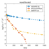
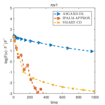
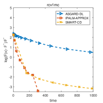
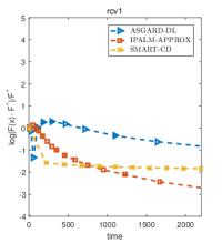
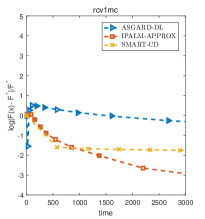
which is also know as Least Absolute Deviation (LAD) problem [44]. We use training data of three different datasets from libsvm [11] as $A$ and modify $b$ such that $Ax=b$ has a sparse solution. We set $\lambda=0.01$. The details about the datasets are given in Table 2. The result is shown in Figure 1. We also compare the time of CVX with IPALM-APPROX to get a mid-level accurate solution in Table 3.

As we can see form Figure 1, IPALM-APPROX has the best performance after accuracy $10^{-3}$. ASGARD-DL works with full dimensional variables and therefore has slow convergence in time. SMART-CD has similar performance as IPALM-APPROX but tends to be slower for obtaining more accurate solution. From Table 3 we can see to get a mid-level accurate solution, IPALM-APPROX significantly outperforms CVX for these three datasets.

Dataset	Training size ($m$)	Number of features ($n$)
news20scale	15,935	62,061
rcv1	20,242	47,236
rcv1mc	15,564	47,236

Table 2: Datasets from libsvm

(a) news20scale

(b) rcv1

(c) rcv1mc

Figure 1: Comparison of three algorithms for LAD problem on three datasets. The $x$-axis is time and $y$-axis is $\log((F(x)-F^{\star})/F^{\star})$. Here we use the result of CVX as an approximation of $F^{\star}$.

Dataset	accuracy (92)	CVX time	IPALM-APPROX time
news20scale	$10^{-5}$	$\sim$4200s	$\sim 500$s
rcv1	$10^{-3}$	$\sim$4000s	$\sim$400s
rcv1mc	$10^{-3}$	$\sim$1800s	$\sim$300s

Table 3: Running time of CVX and IPALM-APPROX for Least absolute deviation problem on three datasets.

7.2 Basis Pursuit

The second problem we solve is of the form:

$$\min_{x\in\mathbb{R}^{n}}\quad \left\|x\right\|_{1}$$

$$s.t.\quad Ax=b$$

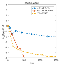
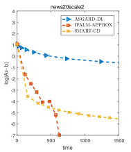
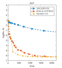
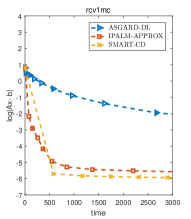
which is known as basis pursuit problem [12]. The datasets used are shown in Table 2 and we modify $b$ for each dataset to make sure that the problem is feasible. The results are shown in Figure 2 for the objective value gap and in Figure 3 for the infeasibility gap. We also compare the time of CVX with IPALM-APPROX to get a mid-level accurate solution in Table 4.

As we can see from Figure 2 and 3, IPALM-APPROX works well both in objective value and feasibility. Since SMART-CD reduces $\beta$ much faster than IPALM-APPROX, it has fast convergence at the beginning, but small $\beta$ leading to small stepsize and slow convergence in objective value for high accuracy. From Table 4, we see the difference between IPALM-APPROX and CVX if only medium accuracy is required.

(a) news20scale

(b) rcv1

(c) rcv1mc

Figure 2: Comparison of three algorithms for basis pursuit problem on three datasets. The $x$-axis is time and $y$-axis is $\log((F(x)-F^{\star})/F^{\star})$. Here we use the result of CVX as an approximation of $F^{\star}$.

(a) news20scale

(b) rcv1

(c) rcv1mc

Figure 3: Comparison of three algorithms for basis pursuit problem on three datasets. The $x$-axis is time and $y$-axis is infeasibility error $\log\|Ax-b\|$.

Dataset	accuracy (92)	CVX time	IPALM-APPROX time
news20scale	$10^{-6}$	$\sim$4200s	$\sim$600s
rcv1	$10^{-2}$	$\sim$2700s	$\sim$1000s
rcv1mc	$10^{-2}$	$\sim$1500s	$\sim$700s

Table 4: Running time of CVX and IPALM-APPROX for basis pursuit problem on three datasets.

7.3 Fused Lasso

The third problem we solve is of the form:

$$\min_{x\in\mathbb{R}^{n}}\frac{1}{2}\left\|Ax-b\right\|_{2}^{2}+\lambda r\left\|x\right\|_{1}+\lambda(1-r)\sum_{i}|x_{i}-x_{i+1}|$$

which is known as Fused Lasso problem [40]. The datasets used are shown in Table 2 and we set $\lambda r=\lambda(1-r)=0.01$.

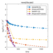
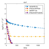
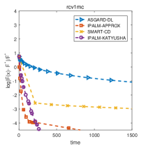
The results are shown in Figure 4 and Table 5. For this problem, we tested both IPALM-APPROX and IPALM-Katyusha. Note that for the datasets in Table 2, we have $n\leq m\leq 2n$ where $m$ is the problem size in (71). According to Table 1, we should expect IPALM-Katyusha to work similarly as IPALM-APPROX, which is indeed observed in practice. Note that in our implementation we used $\tau=\sqrt{m}$ with single processor. Hence the computational time of IPALM-Katyusha can be further reduced when multi-processor and parallel implementation is used.

(a) news20scale

(b) rcv1

(c) rcv1mc

Figure 4: Comparison of four algorithms for Fused Lasso problem on three datasets. The $x$-axis is time and $y$-axis is $\log((F(x)-F^{\star})/F^{\star})$. Here we use the result of CVX as an approximation of $F^{\star}$.

Dataset	accuracy	CVX time	IPALM-APPROX time	IPALM-Katyusha time
news20scale	$10^{-4}$	$\sim$1600s	$\sim$1700s	$\sim 400s$
rcv1	$10^{-4}$	$\sim$7000s	$\sim$300s	$\sim 300$s
rcv1mc	$10^{-4}$	$\sim$5500s	$\sim$400s	$\sim 300$s

Table 5: Running time of CVX, IPALM-APPROX and IPALM-Katyusha for Fused Lasso on three datasets.

As we can see form Figure 4, IPALM-APPROX and IPALM-Katyusha both perform better than ASGARD and SMART-CD. From Table 5, IPALM-Katyusha significantly outperforms CVX to get a mid-level accurate solution for these three datasets.

7.4 Soft Margin SVM

The last problem we solve is of the form:

$$\min_{x\in\mathbb{R}^{n},\omega\in\mathbb{R}}\lambda\left\|x\right\|_{1}+\frac{1}{m}\sum_{i=1}^{m}\max\left(0,1-b_{i}\left(\langle a_{i},x\rangle-\omega\right)\right)$$

which is known as $l_{1}$ regularized soft margin support vector machine problem [49]. Here $a_{i}\in\mathbb{R}^{n}$ are feature vectors and $b_{i}\in\{-1,1\}$ are labels for $i=1,\ldots,m$. We use three different datasets from libsvm [11]. The details about the datasets are given in Table 6.

Dataset	Training size ($m$)	Number of features ($n$)
w4a	7366	300
w8a	49479	300
real-sim	72309	20958

Table 6: Datasets from libsvm

(a) w4a

(b) w8a

(c) real-sim

Figure 5: Comparison of four algorithms for SVM problem on three datasets. The $x$-axis is time and $y$-axis is $\log((F(x)-F^{\star})/F^{\star})$. Here we use the best result of these four algorithms as an approximation of $F^{\star}$.

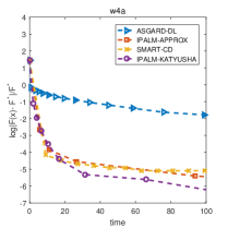
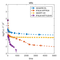
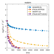
Since here $m\geq n$, we expect IPALM-Katyusha to converge faster than IPALM-APPROX, as indicated by our theoretical bounds given in Table 1. Indeed, as we observe from Figure 5, IPALM-Katyusha has the best performance for all datasets. For w4a and real-sim, the difference of IPALM-Katyusha and IPALM-APPROX is small. But for w8a with $m\gg n$, IPALM-Katyusha significantly outperforms IPALM-APPROX, as well as SMART-CD and ASGARD-DL. Note that for this problem CVX fails so we cannot compare the running time with CVX.

8 Conclusion and Future Research

In this paper we consider a class of structured convex minimization problem and develop an inexact proximal augmented Lagrangian method with explicit inner termination rule. Our framework allows arbitrary linearly convergent inner solver, including in particular many randomized first-order methods. When $p(\cdot)$ is linear, under the same assumptions as [27, 21, 28, 33, 23, 25] but without the boundedness of $\operatorname{dom}(g)$, we obtain nearly optimal $\tilde{O}(1/\epsilon)$ and $\tilde{O}(1/\sqrt{\epsilon})$ complexity bound respectively for the non-strongly convex and strongly convex case. The flexible inner solver choice allows us to deal with large-scale constrained problem more efficiently, with the aid of recent advances in randomized first-order methods for unconstrained problem. We provide numerical evidence showing the efficiency of our approach compared with existing ones when the problem dimension is high.

There are several interesting directions to exploit in the future.

1. The complexity bound established in this paper for non-strongly convex problem is $\tilde{O}(1/\epsilon)$. Throughout the paper we only rely on the fact that the sequence generated by PPA is bounded, whereas it is known that PPA can be linearly convergent if certain metric sub-regularity is satisfied, see e.g. [48]. We expect to obtain a linearly convergent rate under these conditions, see e.g. [22].

2. In numerical experiments, the choice of $\beta_{0}$ does influence the performance. Can a reasonable guess on $\beta_{0}$ be derived from the analysis?

3. When $f$ is only relatively smooth (see Section 5.1.3), we only obtained $\tilde{O}(1/\epsilon^{2})$ and $\tilde{O}(1/\epsilon)$ complexity bound for non-strongly convex and strongly convex case. Can we improve to $\tilde{O}(1/\epsilon)$ and $\tilde{O}(1/\sqrt{\epsilon})$?

4. Can this work be extended to saddle point problem? In particular, [19] discussed an inexact primal-dual method for nonbilinear saddle point problems with bounded $dom(g)$. Can we get rid of the boundedness assumption for saddle point problem?

5. Can this work be extended to weakly convex case as in [13, 35]?

Appendix A Inexact Proximal Point algorithm and inexact Augmented Lagrangian method

A.1 Inexact Proximal Point Method

Let $\mathcal{T}:\mathbb{R}^{n+d}\to\mathbb{R}^{n+d}$ be a maximal monotone operator and $\mathcal{J}_{\rho}=(\mathcal{I}+\rho\mathcal{T})^{-1}$ be the resolvent of $\mathcal{T}$, where $\mathcal{I}$ denotes the identity operator. Then for any $z^{*}$ such that $0\in\mathcal{T}(z^{*})$ [37],

$$\left\|\mathcal{J}_{\rho}(z)-z^{*}\right\|^{2}+\left\|\mathcal{J}_{\rho}(z)-z\right\|^{2}\leq\left\|z-z^{*}\right\|^{2}.$$ (93)

Algorithm 4 PPA

Input: $z_{0}$, $\{\varepsilon_{s}\},\{\rho_{s}\}$.

for $k=0,1,\ldots$ do

     Compute $z^{s+1}\approx\mathcal{J}_{\rho_{s}}(z^{s})$ such that $\left\|z^{s+1}-\mathcal{J}_{\rho_{s}}(z^{s})\right\|\leq\varepsilon_{s}$;

end for

Lemma 11.

[37] Let $\{z^{s}\}$ be the sequence generated by Algorithm 4. Then for any $z^{*}$ such that $0\in\mathcal{T}(z^{*})$,

$$\left\|z^{s+1}-z^{*}\right\|\leq\left\|z_{0}-z^{*}\right\|+\sum_{i=0}^{s}\varepsilon_{i}$$

$$\left\|z^{s+1}-z^{s}\right\|\leq\left\|z_{0}-z^{*}\right\|+\sum_{i=0}^{s}\varepsilon_{i}$$

We now give a stochastic generalization of Algorithm 4.

Algorithm 5 sPPA

Input: $z_{0}$, $\{\varepsilon_{s}\},\{\rho_{s}\}$.

for $k=0,1,\ldots$ do

     Compute $z^{s+1}\approx\mathcal{J}_{\rho_{s}}(z^{s})$ such that $\mathbb{E}\left[\left\|z^{s+1}-\mathcal{J}_{\rho_{s}}(z^{s})\right\|^{2}\right]\leq\varepsilon_{s}^{2}$;

end for

We then extend Lemma 11 for Algorithm 5.

Lemma 12.

Let $\{z^{s}\}$ be the sequence generated by Algorithm 5. Then for any $z^{*}$ such that $0\in\mathcal{T}(z^{*})$,

$$\mathbb{E}\left[\left\|z^{s+1}-z^{*}\right\|\right]\leq\left\|z_{0}-z^{*}\right\|+\sum_{i=0}^{s}\varepsilon_{i}$$

$$\mathbb{E}\left[\left\|z^{s+1}-z^{s}\right\|\right]\leq\left\|z_{0}-z^{*}\right\|+\sum_{i=0}^{s}\varepsilon_{i}$$

$$\left(\mathbb{E}\left[\left\|z^{s+1}-z^{*}\right\|^{2}\right]\right)^{1/2}\leq\left\|z_{0}-z^{*}\right\|+\sum_{i=0}^{s}\varepsilon_{i}$$

Proof.

By the definition of $z^{s}$, we have $\left(\mathbb{E}\left\|z^{s+1}-\mathcal{J}_{\rho_{s}}(z^{s})\right\|\right)^{2}\leq\mathbb{E}\left\|z^{s+1}-\mathcal{J}_{\rho_{s}}(z^{s})\right\|^{2}\leq\varepsilon_{s}^{2}$. The first and second estimates can be obtained by taking expectation on both sides of the result of Lemma 11. The third estimate is derived from $\eqref{PPA}$:

$$0 \leq\left\|\mathcal{J}_{\rho_{s}}-z^{s}\right\|^{2}\leq\left\|z^{s}-z^{*}\right\|^{2}-\left\|\mathcal{J}_{\rho_{s}}(z^{s})-z^{*}\right\|^{2}$$

$$=\left\|z^{s}-z^{*}\right\|^{2}-\left\|\mathcal{J}_{\rho_{s}}(z^{s})-z^{s+1}+z^{s+1}-z^{*}\right\|^{2}$$

$$\leq\left\|z^{s}-z^{*}\right\|^{2}-\left\|z^{s+1}-z^{*}\right\|^{2}-\left\|\mathcal{J}_{\rho_{s}}(z^{s})-z^{s+1}\right\|^{2}+2\left\|\mathcal{J}_{\rho_{s}}(z^{s})-z^{s+1}\right\|\left\|z^{s+1}-z^{*}\right\|$$

Taking expectation on both sides we have:

$$0 \leq\mathbb{E}\left[\left\|z^{s}-z^{*}\right\|^{2}\right]-\mathbb{E}\left[\left\|z^{s+1}-z^{*}\right\|^{2}\right]-\mathbb{E}\left[\left\|\mathcal{J}_{\rho_{s}}(z^{s})-z^{s+1}\right\|^{2}\right]+2\mathbb{E}\left[\left\|\mathcal{J}_{\rho_{s}}(z^{s})-z^{s+1}\right\|\left\|z^{s+1}-z^{*}\right\|\right]$$

$$\leq\mathbb{E}\left[\left\|z^{s}-z^{*}\right\|^{2}\right]-\mathbb{E}\left[\left\|z^{s+1}-z^{*}\right\|^{2}\right]-\mathbb{E}\left[\left\|\mathcal{J}_{\rho_{s}}(z^{s})-z^{s+1}\right\|^{2}\right]+2\left(\mathbb{E}\left[\left\|\mathcal{J}_{\rho_{s}}(z^{s})-z^{s+1}\right\|^{2}\right]\mathbb{E}\left[\left\|z^{s+1}-z^{*}\right\|^{2}\right]\right)^{1/2}$$

$$=\mathbb{E}\left[\left\|z^{s}-z^{*}\right\|^{2}\right]-\left(\left(\mathbb{E}\left[\left\|z^{s+1}-z^{*}\right\|^{2}\right]\right)^{1/2}-\left(\mathbb{E}\left[\left\|\mathcal{J}_{\rho_{s}}(z^{s})-z^{s+1}\right\|^{2}\right]\right)^{1/2}\right)^{2}$$

where the second inequality we use $\mathbb{E}[XY]\leq(\mathbb{E}[X^{2}])^{1/2}(\mathbb{E}[Y^{2}])^{1/2}$. Therefore

$$\left(\mathbb{E}\left[\left\|z^{s+1}-z^{*}\right\|^{2}\right]\right)^{1/2}-\varepsilon_{s}\leq\left(\mathbb{E}\left[\left\|z^{s+1}-z^{*}\right\|^{2}\right]\right)^{1/2}-\left(\mathbb{E}\left[\left\|\mathcal{J}_{\rho_{s}}(z^{s})-z^{s+1}\right\|^{2}\right]\right)^{1/2}\leq\left(\mathbb{E}\left[\left\|z^{s}-z^{*}\right\|^{2}\right]\right)^{1/2}$$

Then summing up the latter inequalities from $s=0$ we obtain the third inequality.

A.2 Inexact ALM

We define the maximal monotone operator $\mathcal{T}_{l}$ as follows.

$$\mathcal{T}_{l}(x;\lambda) =\left\{(v;u):(v;-u)\in\partial L(x;\lambda)\right\}$$

$$=\left\{\begin{pmatrix}\nabla f(x)+\partial g(x)+\nabla p(x)\lambda\\ -p(x)+\partial h^{*}(\lambda)\end{pmatrix}\right\}$$

Recall the definitions in (50). We further let $\Lambda^{\star}(y,\lambda,\beta):=\Lambda(p^{\star}(y,\lambda,\beta);\lambda,\beta)$. By first order optimality condition and (18), we know that

$$0\in\nabla f(x^{\star}(y,\lambda,\beta))+\partial g(x^{\star}(y,\lambda,\beta))+\nabla p(x^{\star}(y,\lambda,\beta))\Lambda^{\star}(y,\lambda,\beta)+\beta(x^{\star}(y,\lambda,\beta)-y)$$

Secondly we know from (23) that

$$p^{\star}(y,\lambda,\beta)-\beta(\Lambda^{\star}(y,\lambda,\beta)-\lambda)\in\partial h^{*}(\Lambda^{\star}(y,\lambda,\beta)).$$

It follows that

$$(\mathcal{I}+\beta^{-1}\mathcal{T}_{l})^{-1}(y;\lambda)=(x^{\star}(y,\lambda,\beta);\Lambda^{\star}(y,\lambda,\beta))$$ (94)

We can then establish the following well known link between inexact ALM and inexact PPA.

Proposition 4 (compare with [37]).

Algorithm 1 is a special case of Algorithm 5 with $\mathcal{T}=\mathcal{T}_{l}$, $\rho_{s}=1/\beta_{s}$ and $\varepsilon_{s}=\sqrt{2\epsilon_{s}/\beta_{s}}$.

Proof.

This follows from (94) and Lemma 7.

Appendix B Missing proofs

B.1 Proofs in Section 2.2

Proof (proof of Lemma 2).

For any $x,y\in\mathbb{R}^{n}$ and $\alpha\in[0,1]$, let $z=\alpha x+(1-\alpha)y$. By condition (15),

$$h\left(p(z)-\alpha u-(1-\alpha)v\right)\leq\alpha h(p(x)-u)+(1-\alpha)h(p(y)-v),\enspace\forall u,v\in\mathbb{R}^{d}.$$

It follows that

$$\tilde{\psi}(z) =\inf_{\omega}\left\{h(p(z)-\omega)+\psi(\omega)\right\}=\inf_{u,v}\left\{h\left(p(z)-\alpha u-(1-\alpha)v\right)+\psi(\alpha u+(1-\alpha)v)\right\}$$

$$\leq\inf_{u,v}\left\{\alpha h(p(x)-u)+(1-\alpha)h(p(y)-v)+\alpha\psi(u)+(1-\alpha)\psi(v)\right\}$$

$$=\alpha\inf_{u}\left\{h(p(x)-u)+\psi(u)\right\}+(1-\alpha)\inf_{v}\left\{h(p(y)-v)+\psi(v)\right\}$$

$$=\alpha\tilde{\psi}(x)+(1-\alpha)\tilde{\psi}(y).$$

Proof (proof of Lemma 3).

The convexity of $\tilde{\psi}$ follows from (20) and Lemma 2 with $\psi(w):=\frac{1}{2\beta}\|w\|^{2}+\langle w,\lambda\rangle$. The gradient formula follows from (18).

Proof (proof of Lemma 4).

This is a direct consequence of Proposition 4 and Lemma 12.

Proof (proof of Corollary 1).

By Lemma 4, we have

$$\mathbb{E}\left[\left\|(x^{s},\lambda^{s+1})-(x^{s-1},\lambda^{s})\right\|\right]\leq\left\|(x^{-1},\lambda^{0})-(x^{\star},\lambda^{\star})\right\|+\frac{2\sqrt{\epsilon_{0}/\beta_{0}}}{1-\sqrt{\eta/\rho}},\enspace\forall s\geq 0,$$

and

$$\mathbb{E}\left[\left\|(x^{s},\lambda^{s+1})-(x^{\star},\lambda^{\star})\right\|^{2}\right]\leq\left(\left\|(x^{-1},\lambda^{0})-(x^{\star},\lambda^{\star})\right\|+\frac{2\sqrt{\epsilon_{0}/\beta_{0}}}{1-\sqrt{\eta/\rho}}\right)^{2},\enspace\forall s\geq 0.$$

Consequently,

$$\mathbb{E}\left[\left\|\lambda^{s+1}-\lambda^{s}\right\|\right]\leq\left\|(x^{-1},\lambda^{0})-(x^{\star},\lambda^{\star})\right\|+\frac{2\sqrt{\epsilon_{0}/\beta_{0}}}{1-\sqrt{\eta/\rho}},\enspace\forall s\geq 0,$$

and

$$\max\left(\mathbb{E}\left[\left\|x^{s}-x^{\star}\right\|^{2}\right],\mathbb{E}\left[\left\|\lambda^{s+1}-\lambda^{\star}\right\|^{2}\right]\right)\leq\left(\left\|(x^{-1},\lambda^{0})-(x^{\star},\lambda^{\star})\right\|+\frac{2\sqrt{\epsilon_{0}/\beta_{0}}}{1-\sqrt{\eta/\rho}}\right)^{2},\enspace\forall s\geq 0.$$

We then conclude.

Proof (proof of Theorem 1).

First,

$$\begin{array}[]{ll}h_{1}(p_{1}(x^{s}))-h(p(x^{s});\lambda^{s},\beta_{s})&\overset{\eqref{a:hbeta}}{=}h_{1}(p_{1}(x^{s}))-h_{1}(p_{1}(x^{s})-\beta_{s}(\lambda_{1}^{s+1}-\lambda_{1}^{s}))-\frac{\beta_{s}}{2}(\|\lambda^{s+1}\|^{2}-\|\lambda^{s}\|^{2})\\ &\leq L_{h_{1}}\beta_{s}\|\lambda^{s+1}-\lambda^{s}\|+\frac{\beta_{s}}{2}(\|\lambda^{s}\|^{2}-\|\lambda^{s+1}\|^{2}).\end{array}$$ (95)

Then we know that

$$F(x^{s})-L(x^{s};x^{s-1},\lambda^{s},\beta_{s}) =h_{1}(p_{1}(x^{s}))-h(p(x^{s});\lambda^{s},\beta_{s})-\frac{\beta_{s}}{2}\|x^{s}-x^{s-1}\|^{2}$$

$$\overset{\eqref{eq:fsr}}{\leq}L_{h_{1}}\beta_{s}\|\lambda^{s+1}-\lambda^{s}\|+\frac{\beta_{s}}{2}(\|\lambda^{s}\|^{2}-\|\lambda^{s+1}\|^{2})-\frac{\beta_{s}}{2}\|x^{s}-x^{s-1}\|^{2}.$$

Since $H_{s}(\cdot)$ is $\beta_{s}$-strongly convex, we know that

$$L^{\star}(x^{s-1},\lambda^{s},\beta_{s}) \leq L(x^{\star};x^{s-1},\lambda^{s},\beta^{s})-\frac{\beta_{s}}{2}\|x^{\star}-x^{\star}(x^{s-1},\lambda^{s},\beta_{s})\|^{2}$$

$$\overset{\eqref{a:dualityhbeta}}{\leq}F^{\star}+\frac{\beta_{s}}{2}\|x^{\star}-x^{s-1}\|^{2}-\frac{\beta_{s}}{2}\|x^{\star}-x^{\star}(x^{s-1},\lambda^{s},\beta_{s})\|^{2}.$$

Combining the latter two bounds we get

$$F(x^{s})-F^{\star} \leq L(x^{s};x^{s-1},\lambda^{s},\beta_{s})-L^{\star}(x^{s-1},\lambda^{s},\beta_{s})+L_{h_{1}}\beta_{s}\|\lambda^{s+1}-\lambda^{s}\|+\frac{\beta_{s}}{2}(\|\lambda^{s}\|^{2}-\|\lambda^{s+1}\|^{2})$$

$$\quad+\frac{\beta_{s}}{2}\|x^{\star}-x^{s-1}\|^{2}-\frac{\beta_{s}}{2}\|x^{\star}-x^{\star}(x^{s-1},\lambda^{s},\beta_{s})\|^{2}-\frac{\beta_{s}}{2}\|x^{s}-x^{s-1}\|^{2}.$$

Furthermore, by convexity of $h_{1}(\cdot)$,

$$\inf_{x}F(x)+\langle\lambda_{2}^{\star},p_{2}(x)\rangle-h_{2}^{*}(\lambda_{2}^{\star})\geq\inf_{x}f(x)+g(x)+\langle\lambda^{\star},p(x)\rangle-h^{*}(\lambda^{\star})=D(\lambda^{\star}).$$

Now we apply the strong duality assumption (11) to obtain:

$$F(x^{s})+\langle\lambda_{2}^{\star},p_{2}(x^{s})\rangle-h_{2}^{*}(\lambda_{2}^{\star})\geq\inf_{x}F(x)+\langle\lambda_{2}^{\star},p_{2}(x)\rangle-h_{2}^{*}(\lambda_{2}^{\star})\geq F^{\star}.$$

Consequently,

$$F(x^{s})-F^{\star}\geq\langle\lambda_{2}^{\star},-p_{2}(x^{s})\rangle+h_{2}^{*}(\lambda_{2}^{\star})\geq\sup_{v}\langle\lambda_{2}^{\star},v-p_{2}(x^{s})\rangle-h_{2}(v)\geq-\|\lambda_{2}^{\star}\|\operatorname{dist}(p_{2}(x^{s}),\mathcal{K}).$$

From (23) we know

$$p_{2}(x^{s})-\beta_{s}(\lambda_{2}^{s+1}-\lambda_{2}^{s})\in\mathcal{K},$$

and thus

$$\operatorname{dist}(p_{2}(x^{s}),\mathcal{K})\leq\beta_{s}\|\lambda_{2}^{s+1}-\lambda_{2}^{s}\|.$$

Proof (proof of Corollary 2).

Using Corollary 1, the bounds in Theorem 1 can be relaxed as:

$$\mathbb{E}[F(x^{s})-F^{\star}]\leq\epsilon_{s}+2L_{h_{1}}^{2}\beta_{s}+c_{0}\beta_{s}$$

$$\mathbb{E}[F(x^{s})-F^{\star}]\geq-\beta_{s}\|\lambda_{2}^{\star}\|\sqrt{c_{0}},$$

$$\mathbb{E}[\operatorname{dist}(p_{2}(x^{s}),K)]\leq\beta_{s}\sqrt{c_{0}}.$$

We then conclude by noting that (32) guarantees

$$\max(\epsilon_{0}+2L_{h_{1}}^{2}\beta_{0}+c_{0}\beta_{0},\beta_{0}\|\lambda_{2}^{\star}\|\sqrt{c_{0}},\beta_{0}\sqrt{c_{0}})\leq\epsilon\rho^{-s}.$$

B.2 Proofs in Section 3.2

Proof (proof of Lemma 5).

We first bound

$$\mathbb{E}[\left((\beta_{s}+\beta_{s+1})L_{h_{1}}+\|\beta_{s}\lambda_{1}^{s}-\beta_{s+1}\lambda_{1}^{s+1}\|\right)^{2}+\|\beta_{s}\lambda_{2}^{s}-\beta_{s+1}\lambda_{2}^{s+1}\|^{2}]$$

$$\leq 2(\beta_{s}+\beta_{s+1})^{2}L^{2}_{h_{1}}+2\mathbb{E}[\|\beta_{s}\lambda^{s}-\beta_{s+1}\lambda^{s+1}\|^{2}]$$

$$\leq 2(\beta_{s}+\beta_{s+1})^{2}L^{2}_{h_{1}}+4(\beta_{s}^{2}+\beta_{s+1}^{2})c$$

$$\leq 4(\beta_{s}^{2}+\beta_{s+1}^{2})(L^{2}_{h_{1}}+c).$$

Since

$$\lambda^{s+1}=\Lambda(p(x^{s});\lambda^{s},\beta_{s}),$$

by Lemma 8 we have

$$\|\beta_{s+1}\left(\Lambda(p(x^{s});\lambda^{s+1},\beta_{s+1})-\lambda^{s+1}\right)-\beta_{s}(\lambda^{s+1}-\lambda^{s})\|$$ (96)

$$\leq\sqrt{\left((\beta_{s}+\beta_{s+1})L_{h_{1}}+\|\beta_{s}\lambda_{1}^{s}-\beta_{s+1}\lambda_{1}^{s+1}\|\right)^{2}+\|\beta_{s}\lambda_{2}^{s}-\beta_{s+1}\lambda_{2}^{s+1}\|^{2}}\enspace.$$ (97)

Therefore,

$$\|\Lambda(p(x^{s});\lambda^{s+1},\beta_{s+1})-\lambda^{s+1}\|$$

$$\leq\beta_{s+1}^{-1}\beta_{s}\|\lambda^{s+1}-\lambda^{s}\|+\beta_{s+1}^{-1}\sqrt{\left((\beta_{s}+\beta_{s+1})L_{h_{1}}+\|\beta_{s}\lambda_{1}^{s}-\beta_{s+1}\lambda_{1}^{s+1}\|\right)^{2}+\|\beta_{s}\lambda_{2}^{s}-\beta_{s+1}\lambda_{2}^{s+1}\|^{2}}.$$

If follows that

$$\mathbb{E}[\|\Lambda(p(x^{s});\lambda^{s+1},\beta_{s+1})-\lambda^{s+1}\|^{2}]\leq 2\beta_{s+1}^{-2}\beta^{2}_{s}c+8\beta_{s+1}^{-2}(\beta_{s}^{2}+\beta_{s+1}^{2})(L^{2}_{h_{1}}+c)$$ (98)

By $\mathbb{E}[XY]\leq(\mathbb{E}[X^{2}])^{1/2}(\mathbb{E}[Y^{2}])^{1/2}$, we get

$$\mathbb{E}\left[\|\lambda^{s+1}-\lambda^{s}\|\sqrt{\left((\beta_{s}+\beta_{s+1})L_{h_{1}}+\|\beta_{s}\lambda_{1}^{s}-\beta_{s+1}\lambda_{1}^{s+1}\|\right)^{2}+\|\beta_{s}\lambda_{2}^{s}-\beta_{s+1}\lambda_{2}^{s+1}\|^{2}}\right]\leq\sqrt{4c(\beta_{s}^{2}+\beta_{s+1}^{2})(L^{2}_{h_{1}}+c)}.$$ (99)

Combining (41), (98) and (99), we then get an upper bound for $\mathbb{E}[M_{s}]$:

$$\begin{array}[]{ll}\mathbb{E}[M_{s+1}]&\leq{{\beta_{s}}}c+\frac{\beta_{s}-\beta_{s+1}}{2}\left(2\beta_{s+1}^{-2}\beta^{2}_{s}c+8\beta_{s+1}^{-2}(\beta_{s}^{2}+\beta_{s+1}^{2})(L^{2}_{h_{1}}+c)\right)+\frac{\beta_{s}^{2}}{2\beta_{s+1}-\beta_{s}}c+\sqrt{4c(\beta_{s}^{2}+\beta_{s+1}^{2})(L^{2}_{h_{1}}+c)}\\ &\leq{{\beta_{s}}}c+\beta_{s}\left(\beta_{s+1}^{-2}\beta^{2}_{s}c+4\beta_{s+1}^{-2}(\beta_{s}^{2}+\beta_{s+1}^{2})(L^{2}_{h_{1}}+c)\right)+\frac{\beta_{s}^{2}}{2\beta_{s+1}-\beta_{s}}c+2\beta_{s}\sqrt{c(1+\beta_{s+1}^{2}\beta_{s}^{-2})(L^{2}_{h_{1}}+c)}\\ &\leq 2{{\beta_{s}}}c+\beta_{s}\left(\beta_{s+1}^{-2}\beta^{2}_{s}c+(5+4\beta_{s+1}^{-2}\beta_{s}^{2}+\beta_{s+1}^{2}\beta_{s}^{-2})(L^{2}_{h_{1}}+c)\right)+\frac{\beta_{s}^{2}}{2\beta_{s+1}-\beta_{s}}c\end{array},$$

where the last inequality used $2\sqrt{ab}\leq a+b$ for any $a,b>0$. Next we plug in $\beta_{s}=\beta_{0}\rho^{s}$ to obtain

$$\mathbb{E}[M_{s}]\leq\beta_{s}\left(2c+\rho^{-2}c+(9+\rho^{-2})(L^{2}_{h_{1}}+c)+(2\rho-1)^{-1}c\right)\leq\beta_{s}\left((11+2\rho^{-2})(L^{2}_{h_{1}}+c)+(2\rho-1)^{-1}c\right).$$

Proof (proof of Proposition 2).

Since Algorithm 2 is a special case of Algorithm 1 with $\beta_{s}=\beta_{0}\rho^{s}$ and $\epsilon_{s}=\epsilon_{0}\eta^{s}$, we know from Corollary 1 that (41) holds with $c=4c_{0}$. Applying Lemma 5 we know that

$$\mathbb{E}[M_{s}]\leq C\beta_{s},$$

with $C=(11+2\rho^{-2})(L^{2}_{h_{1}}+4c_{0})+4(2\rho-1)^{-1}c_{0}$. If $m_{s+1}$ is the smallest integer satisfying (37), then

$$m_{s+1}\leq K_{s+1}\left(\log_{2}\left(4\epsilon_{s}\epsilon^{-1}_{s+1}+2M_{s}\epsilon^{-1}_{s+1}\right)+1\right)+1.$$ (100)

By the concavity of $\log_{2}$ function we get

$$\mathbb{E}[m_{s+1}]\leq K_{s+1}\left(\log_{2}\left(4\epsilon_{s}\epsilon^{-1}_{s+1}+2C\beta_{s}\epsilon^{-1}_{s+1}\right)+1\right)+1=K_{s+1}\left(\log_{2}\left(4\eta^{-1}+2C\beta_{0}\epsilon_{0}^{-1}\eta^{-1}\rho^{s}\eta^{-s}\right)+1\right)+1.$$

Since $\rho>\eta$, we get

$$\mathbb{E}[m_{s+1}] \leq K_{s+1}\left(\log_{2}\left(\left(4\eta^{-1}+2C\beta_{0}\epsilon_{0}^{-1}\eta^{-1}\right)\rho^{s}\eta^{-s}\right)+1\right)+1$$

$$=K_{s+1}\left(\log_{2}\left(4\eta^{-1}+2C\beta_{0}\epsilon_{0}^{-1}\eta^{-1}\right)+1+\log_{2}\left(\rho^{s}\eta^{-s}\right)\right)+1$$

$$=K_{s+1}\left(s\log_{2}\left(\rho\eta^{-1}\right)+c_{2}\right)+1.$$

B.3 Proofs in Section 3.3

We first state a lemma similar to Lemma 2.

Lemma 13.

Let $\psi(\cdot):\mathbb{R}^{n}\rightarrow\mathbb{R}\cup\{+\infty\}$ be a convex function. Define:

$$\tilde{\psi}(w):=\inf_{x}\{h(p(x)-w)+\psi(x)\},$$

Then condition (15) ensures the convexity of $\tilde{\psi}$.

Proof.

The proof is similar to Lemma 2 in Appendix B.1.

Proof (proof of Lemma 6).

By the definitions (24), (16) and (17), we have

$$L(x;y,\lambda,\beta)-L(x;y^{\prime},\lambda^{\prime},\beta^{\prime})+\frac{\beta}{2}\|\Lambda(p(x);\lambda,\beta)-\lambda\|^{2}-\frac{\beta^{\prime}}{2}\|\Lambda(p(x);\lambda^{\prime},\beta^{\prime})-\lambda^{\prime}\|^{2}$$

$$=\langle\Lambda(p(x);\lambda,\beta)-\Lambda(p(x);\lambda^{\prime},\beta^{\prime}),p(x)\rangle-h^{*}(\Lambda(p(x);\lambda,\beta))+h^{*}(\Lambda(p(x);\lambda^{\prime},\beta^{\prime}))+\frac{\beta}{2}\|x-y\|^{2}-\frac{\beta^{\prime}}{2}\|x-y^{\prime}\|^{2}.$$

Next we apply (23) to get

$$h^{*}(\Lambda(p(x);\lambda^{\prime},\beta^{\prime}))\geq h^{*}(\Lambda(p(x);\lambda,\beta))+\langle\Lambda(p(x);\lambda,\beta)-\Lambda(p(x);\lambda^{\prime},\beta^{\prime}),\beta(\Lambda(p(x);\lambda,\beta)-\lambda)-p(x)\rangle,$$

and

$$h^{*}(\Lambda(p(x);\lambda,\beta))\geq h^{*}(\Lambda(p(x);\lambda^{\prime},\beta^{\prime}))+\langle\Lambda(p(x);\lambda,\beta)-\Lambda(p(x);\lambda^{\prime},\beta^{\prime}),p(x)-\beta^{\prime}(\Lambda(p(x);\lambda^{\prime},\beta^{\prime})-\lambda^{\prime})\rangle.$$

Proof (proof of Lemma 7).

In this proof we fix $y\in\mathbb{R}^{n}$, $\lambda\in\mathbb{R}^{d}$ and $\beta>0$. Recall the definitions in (50). Define

$$L(x,w;y,\lambda,\beta):=f(x)+g(x)+h(p(x)-w)+\frac{1}{2\beta}\|w\|^{2}+\langle w,\lambda\rangle+\frac{\beta}{2}\|x-y\|^{2}-\frac{\beta}{2}\|x-x^{\star}(y,\lambda,\beta)\|^{2}.$$

Then by (20),

$$\min_{w}L(x,w;y,\lambda,\beta)=L(x;y,\lambda,\beta)-\frac{\beta}{2}\|x-x^{\star}(y,\lambda,\beta)\|^{2}.$$ (101)

Since $L(x;y,\lambda,\beta)-\frac{\beta}{2}\|x-x^{\star}(y,\lambda,\beta)\|^{2}$ is a convex function with $x^{\star}(y,\lambda,\beta)$ being a critical point, it follows that

$$\min_{x}\min_{w}L(x,w;y,\lambda,\beta)=L^{\star}(y,\lambda,\beta).$$ (102)

Denote

$$H(w;y,\lambda,\beta):=\min_{x}L(x,w;y,\lambda,\beta).$$ (103)

In view of (21),

$$L(x;y,\lambda,\beta)-\frac{\beta}{2}\|x-x^{\star}(y,\lambda,\beta)\|^{2}=L(x,\beta(\Lambda(p(x);\lambda,\beta)-\lambda);y,\lambda,\beta)\overset{\eqref{a:Hdef}}{\geq}H(\beta(\Lambda(p(x);\lambda,\beta)-\lambda);y,\lambda,\beta).$$ (104)

Note that

$$\min_{w}H(w;y,\lambda,\beta)=\min_{w}\min_{x}L(x,w;y,\lambda,\beta)=\min_{x}\min_{w}L(x,w;y,\lambda,\beta)\overset{\eqref{a:poi}}{=}L^{\star}(y,\lambda,\beta).$$ (105)

Denote $\Lambda^{\star}(y,\lambda,\beta)=\Lambda(p^{\star}(y,\lambda,\beta);\lambda,\beta)$. It follows that,

$$H(\beta(\Lambda^{\star}(y,\lambda,\beta)-\lambda);y,\lambda,\beta)\geq\min_{w}H(w;y,\lambda,\beta)\overset{\eqref{a:efwq}}{=}L^{\star}(y,\lambda,\beta)=L(x^{\star}(y,\lambda,\beta);y,\lambda,\beta).$$

Using again (104) with $x=x^{\star}(y,\lambda,\beta)$ we deduce

$$H(\beta(\Lambda^{\star}(y,\lambda,\beta)-\lambda);y,\lambda,\beta)=\min_{w}H(w;y,\lambda,\beta).$$ (106)

Moreover, it follows from Lemma 13 that $H(w;y,\lambda,\beta)$ is $1/\beta$-strongly convex with respect to $w$. Thus,

$$L(x;y,\lambda,\beta)-L^{\star}(y,\lambda,\beta)-\frac{\beta}{2}\|x-x^{\star}(y,\lambda,\beta)\|^{2} \overset{\eqref{a:rtdffrtr}+\eqref{a:efwq}}{\geq}H(\beta(\Lambda(p(x);\lambda,\beta)-\lambda);y,\lambda,\beta)-\min_{w}H(w;y,\lambda,\beta)$$

$$\overset{\eqref{a:rqqsf}}{\geq}\frac{1}{2\beta}\|\beta(\Lambda(p(x);\lambda,\beta)-\lambda)-\beta(\Lambda^{\star}(y,\lambda,\beta)-\lambda)\|^{2}$$

$$=\frac{\beta}{2}\|\Lambda(p(x);\lambda,\beta)-\Lambda^{\star}(y,\lambda,\beta)\|^{2}.$$

Proof (proof of Lemma 8).

Denote

$$\Lambda_{i}(u_{i};\lambda_{i},\beta):=\arg\max_{\xi_{i}}\left\{\langle\xi_{i},u_{i}\rangle-h_{i}^{*}(\xi_{i})-\frac{\beta}{2}\|\xi_{i}-\lambda_{i}\|^{2}\right\},\enspace i=1,2,$$ (107)

so that $\Lambda(u;\lambda,\beta)=\left(\Lambda_{1}(u_{1};\lambda_{1},\beta);\Lambda_{2}(u_{2};\lambda_{2},\beta)\right)$. We can then decompose (23) into two independent conditions:

$$\Lambda_{i}(u_{i};\lambda_{i},\beta)\in\partial h_{i}(u_{i}-\beta(\Lambda_{i}(u_{i};\lambda_{i},\beta)-\lambda_{i})),\enspace i=1,2.$$ (108)

By condition (a) in Assumption 1,

$$\|\Lambda_{1}(u_{1};\lambda_{1},\beta)\|\leq L_{h_{1}}$$ (109)

which yields directly

$$\|\beta(\Lambda_{1}(u_{1};\lambda_{1},\beta)-\lambda_{1})-\beta^{\prime}(\Lambda_{1}(u_{1};\lambda_{1}^{\prime},\beta^{\prime})-\lambda_{1}^{\prime})\|\leq(\beta+\beta^{\prime})L_{h_{1}}+\|\beta\lambda_{1}-\beta^{\prime}\lambda_{1}^{\prime}\|.$$ (110)

On the other hand, since $h_{2}$ is an indicator function, $\partial h_{2}$ is a cone and (108) implies

$$\beta\Lambda_{2}(u_{2};\lambda_{2},\beta)\in\partial h_{2}(u_{2}-\beta(\Lambda_{2}(u_{2};\lambda_{2},\beta)-\lambda_{2})).$$ (111)

The latter condition further leads to

$$\langle\beta\Lambda_{2}(u_{2};\lambda_{2},\beta)-\beta^{\prime}\Lambda_{2}(u_{2};\lambda^{\prime}_{2},\beta^{\prime}),\beta(\Lambda_{2}(u_{2};\lambda_{2},\beta)-\lambda_{2})-\beta^{\prime}(\Lambda_{2}(u_{2};\lambda_{2}^{\prime},\beta^{\prime})-\lambda_{2}^{\prime})\rangle\leq 0,$$

which by Cauchy-Schwartz inequality implies

$$\|\beta(\Lambda_{2}(u_{2};\lambda_{2},\beta)-\lambda_{2})-\beta^{\prime}(\Lambda_{2}(u_{2};\lambda^{\prime}_{2},\beta^{\prime})-\lambda_{2}^{\prime})\|\leq\|\beta\lambda_{2}-\beta^{\prime}\lambda_{2}^{\prime}\|.$$

Then (54) is obtained by simple algebra.

Proof (proof of Lemma 9).

We first recall the following basic inequality:

$$\|u+v\|^{2}\leq(1+a)\|u\|^{2}+(1+1/a)\|v\|^{2},\enspace\forall u,v\in\mathbb{R}^{n},a>0.$$ (112)

In view of (112) and the fact that $\beta^{\prime}>\beta/2$, we know that

$$-\frac{\beta}{2}\|w^{\prime}-w\|^{2}\leq\frac{\beta}{2}\|w-y^{\prime}\|^{2}-\frac{\beta}{4}\|w^{\prime}-y^{\prime}\|^{2},$$

$$-\frac{\beta^{\prime}+\beta/2}{2}\|w^{\prime}-y^{\prime}\|^{2}\leq\frac{\beta(2\beta^{\prime}+\beta)}{2(2\beta^{\prime}-\beta)}\|y-y^{\prime}\|^{2}-\frac{\beta}{2}\|w^{\prime}-y\|^{2}.$$

Combining the latter two inequalities we get (55).

B.4 Proof in Section 5.1

Proof (proof of Corollary 5).

If $K_{s}$ satisfies (69), then

$$K_{s}\leq 2\sqrt{\frac{2(L\beta_{0}+\|A\|^{2})}{\mu_{g}\beta_{s}+\beta^{2}_{s}}}+1\leq\left\{\begin{array}[]{ll}\frac{2\sqrt{2(L\beta_{0}+\|A\|^{2})/\mu_{g}}}{\sqrt{\beta_{s}}}+1&\mathrm{if}~{}\mu_{g}>0\\ \frac{2\sqrt{2(L\beta_{0}+\|A\|^{2})}}{{\beta_{s}}}+1&\mathrm{if}~{}\mu_{g}=0\end{array}\right.$$

We then apply Corollary 4.

The proof of Corollary 6 and 7 are similar.

B.5 Proofs in Section 5.2

We first state a useful Lemma.

Lemma 14.

For any $u,\lambda\in\mathbb{R}^{d}$, $\beta>0$,

$$\|\Lambda(u;\lambda,\beta)\|\leq L_{h_{1}}+\beta^{-1}\operatorname{dist}(u_{2}+\beta\lambda_{2},\mathcal{K})$$ (113)

Proof.

From (20),

$$h(u;\lambda,\beta)=\min_{z}\left\{h(z)+\frac{1}{2\beta}\|u+\beta\lambda-z\|^{2}-\frac{\beta}{2}\|\lambda\|^{2}\right\}$$ (114)

with optimal solution

$$z^{*}=u+\beta\lambda-\beta\Lambda(u;\lambda,\beta).$$

In particular, $\operatorname{dist}(u_{2}+\beta\lambda_{2},\mathcal{K})^{2}=\beta^{2}\|\Lambda_{2}(u_{2};\lambda_{2},\beta)\|^{2}$. Together with (109) we obtain the desired bound.

Proof (proof of Lemma 10).

$$\|\nabla p(x)\Lambda(p(x);\lambda^{s},\beta_{s})-\nabla p(y)\Lambda(p(y);\lambda^{s},\beta_{s})\|$$

$$\leq\|\nabla p(x)-\nabla p(y)\|\|\Lambda(p(x);\lambda^{s},\beta_{s})\|+\|\nabla p(y)\|\|\Lambda(p(x);\lambda^{s},\beta_{s})-\Lambda(p(y);\lambda^{s},\beta_{s})\|$$

$$\overset{\eqref{a:ewssss}+\eqref{a:nablahLip}}{\leq}L_{\nabla p}\|x-y\|\left(L_{h_{1}}+\beta_{s}^{-1}\operatorname{dist}(p_{2}(x)+\beta_{s}\lambda^{s}_{2},\mathcal{K})\right)+M_{\nabla p}\|p(x)-p(y)\|\beta_{s}^{-1}$$

$$\leq\left(L_{\nabla p}\left(L_{h_{1}}+\beta_{s}^{-1}\operatorname{dist}(p_{2}(x)+\beta_{s}\lambda^{s}_{2},\mathcal{K})\right)+M^{2}_{\nabla p}\beta_{s}^{-1}\right)\|x-y\|.$$

Note that by (81) and the definition of $d_{s}$,

$$\operatorname{dist}(p_{2}(x)+\beta_{s}\lambda_{2}^{s},\mathcal{K})\leq d_{s}.$$

B.6 Proofs in Section 6.2

Proof (proof of Theorem 3).

We know from the basic property of proximal gradient step [31] that

$$\|x^{s}-\tilde{x}^{s}\|^{2}\leq 2\left(H_{s}(\tilde{x}^{s})-H_{s}^{\star}\right)/L_{s}.$$

By Line 4 in Algorithm 3,

$$0\in\nabla\phi_{s}(\tilde{x}^{s})+L_{s}(x^{s}-\tilde{x}^{s})+{\beta_{s}}(x^{s}-x^{s-1})+\partial g(x^{s}).$$

Therefore,

$$\operatorname{dist}(0,\nabla\phi_{s}(x^{s})+\partial g(x^{s})) \leq L_{s}\|\tilde{x}^{s}-x^{s}\|+\|\nabla\phi_{s}(x^{s})-\nabla\phi_{s}(\tilde{x}^{s})\|+\beta_{s}\|x^{s}-x^{s-1}\|$$

$$\leq 2L_{s}\|\tilde{x}^{s}-x^{s}\|+\beta_{s}\|x^{s}-x^{s-1}\|$$

Combining the last two bounds and (18) we get $\nabla\phi_{s}(x^{s})=\nabla f(x^{s})+\nabla p(x^{s})\lambda^{s+1}$ and

$$\operatorname{dist}(0,\nabla f(x^{s})+\nabla p(x^{s})\lambda^{s+1}+\partial g(x^{s}))^{2}\leq 16L_{s}\left(H_{s}(\tilde{x}^{s})-H_{s}^{\star}\right)+2\beta_{s}^{2}\|x^{s}-x^{s-1}\|^{2}.$$

Secondly we know from (23) that

$$p(x^{s})-\beta_{s}(\lambda^{s+1}-\lambda^{s})\in\partial h^{*}(\lambda^{s+1}).$$

It follows that

$$\operatorname{dist}(0,p(x^{s})-\partial h^{*}(\lambda^{s+1}))\leq\beta_{s}\|\lambda^{s+1}-\lambda^{s}\|.$$

Proof (proof of Corollary 9).

Due to (87), we can have the same bound (in expectation) of the sequence $\{(\tilde{x}^{s},x^{s},\lambda^{s})\}$ as Corollary 1. Hence,

$$\mathbb{E}\left[\operatorname{dist}(0,\partial_{x}L(x^{s},\lambda^{s+1}))\right]\leq\sqrt{16L_{s}\epsilon_{s}+8c_{0}\beta_{s}^{2}}\leq\sqrt{16\gamma\epsilon_{0}/\beta_{0}+8c_{0}\beta_{0}}\rho^{s},$$

$$\mathbb{E}\left[\operatorname{dist}(0,\partial_{\lambda}L(x^{s},\lambda^{s+1}))\right]\leq\beta_{0}\sqrt{c_{0}}\rho^{s}.$$

References

- [1] A. Alacaoglu, Q. Tran-Dinh, O. Fercoq, and V. Cevher. Smooth primal-dual coordinate descent algorithms for nonsmooth convex optimization. In Advances in Neural Information Processing Systems, pages 5852–5861, 2017.
- [2] Z. Allen-Zhu. Katyusha: The first direct acceleration of stochastic gradient methods. In The Journal of Machine Learning Research, volume 18(1), pages 8194–8244, 2017.
- [3] A. Auslender and M. Teboulle. Interior Projection-like Methods for Monotone Variational Inequalities. Math. Program., 104(1):39–68, Sept. 2005.
- [4] A. Beck and M. Teboulle. A fast iterative shrinkage-thresholding algorithm for linear inverse problems. SIAM Journal on Imaging Sciences, 2(1):183–202, 2009.
- [5] A. Beck and M. Teboulle. Smoothing and First Order Methods: A Unified Framework. SIAM Journal on Optimization, 22(2):557–580, 2012.
- [6] A. Belloni, V. Chernozhukov, and L. Wang. Square-Root lasso: Pivotal Recovery of Sparse Signals via Conic Programming. SSRN Electronic Journal, 01 2011.
- [7] D. P. Bertsekas. Constrained optimization and Lagrange multiplier methods. Academic press, 2014.
- [8] J. Bolte, H. H. Bauschke, and M. Teboulle. A Descent Lemma Beyond Lipschitz Gradient Continuity: First-Order Methods Revisited and Applications. Mathematics of Operations Research, 42, 07 2016.
- [9] A. Chambolle, M. J. Ehrhardt, P. Richtárik, and C.-B. Schonlieb. Stochastic primal-dual hybrid gradient algorithm with arbitrary sampling and imaging applications. SIAM Journal on Optimization, 28(4):2783–2808, 2018.
- [10] A. Chambolle and T. Pock. A first-order primal-dual algorithm for convex problems with applications to imaging. Journal of mathematical imaging and vision, 40(1):120–145, 2011.
- [11] C.-C. Chang and C.-J. Lin. LIBSVM: A library for support vector machines. ACM transactions on intelligent systems and technology (TIST), 2(3):27, 2011.
- [12] S. Chen, D. Donoho, and M. Saunders. Atomic Decomposition by Basis Pursuit. SIAM Journal on Scientific Computing, 20(1):33–61, 1998.
- [13] D. Drusvyatskiy and C. Paquette. Efficiency of minimizing compositions of convex functions and smooth maps. Mathematical Programming, pages 1–56.
- [14] O. Fercoq and Z. Qu. Restarting the accelerated coordinate descent method with a rough strong convexity estimate. arXiv:1803.05771, 2018.
- [15] O. Fercoq and Z. Qu. Adaptive restart of accelerated gradient methods under local quadratic growth condition. IMA Journal of Numerical Analysis, 03 2019.
- [16] O. Fercoq and P. Richtárik. Accelerated, parallel and proximal coordinate descent. SIAM Journal on Optimization, 25(4):1997–2023, 2015.
- [17] M. P. Friedlander and G. Goh. Efficient evaluation of scaled proximal operators. Electronic Transactions on Numerical Analysis, 46:1–22, 2017.
- [18] H. H. Bauschke and P. Combettes. The baillon-haddad theorem revisited. Journal of Convex Analysis, 17, 06 2009.
- [19] L. T. K. Hien, R. Zhao, and W. B. Haskell. An inexact primal-dual smoothing framework for large-scale non-bilinear saddle point problems. arXiv preprint arXiv:1711.03669, 2017.
- [20] D. Kovalev, S. Horváth, and P. Richtárik. Don’t Jump Through Hoops and Remove Those Loops: SVRG and Katyusha are Better Without the Outer Loop. 2019.
- [21] G. Lan and R. D. Monteiro. Iteration-complexity of First-order Augmented Lagrangian Methods for Convex Programming. Math. Program., 155(1-2):511–547, Jan. 2016.
- [22] H. Li and Z. Lin. On the Complexity Analysis of the Primal Solutions for the Accelerated Randomized Dual Coordinate Ascent. arXiv preprint arXiv:1807.00261, 2018.
- [23] Y. Liu, X. Liu, and S. Ma. On the Nonergodic Convergence Rate of an Inexact Augmented Lagrangian Framework for Composite Convex Programming. Mathematics of Operations Research, 44(2):632–650, 2019.
- [24] H. Lu, R. Freund, and Y. Nesterov. Relatively Smooth Convex Optimization by First-Order Methods, and Applications. SIAM Journal on Optimization, 28(1):333–354, 2018.
- [25] Z. Lu and Z. Zhou. Iteration-complexity of first-order augmented Lagrangian methods for convex conic programming. arXiv preprint arXiv:1803.09941, 2018.
- [26] I. Necoara, Y. Nesterov, and F. Glineur. Linear convergence of first order methods for non-strongly convex optimization. Mathematical Programming, Jan 2018.
- [27] I. Necoara, A. Patrascu, and F. Glineur. Complexity of first-order inexact Lagrangian and penalty methods for conic convex programming. Optimization Methods and Software, 34(2):305–335, 2019.
- [28] V. Nedelcu, I. Necoara, and Q. Tran-Dinh. Computational Complexity of Inexact Gradient Augmented Lagrangian Methods: Application to Constrained MPC. SIAM Journal on Control and Optimization, 52(5):3109–3134, 2014.
- [29] Y. Nesterov. A method of solving a convex programming problem with convergence rate . Soviet Mathematics Doklady, 27(2):372–376, 1983.
- [30] Y. Nesterov. Smooth minimization of non-smooth functions. Mathematical Programming, 103(1):127–152, May 2005.
- [31] Y. Nesterov et al. Gradient methods for minimizing composite objective function, 2007.
- [32] Y. Ouyang, Y. Chen, G. Lan, and E. P. Jr. An accelerated linearized alternating direction method of multipliers. SIAM Journal on Imaging Sciences, 8(1):644–681, 2015.
- [33] A. Patrascu, I. Necoara, and Q. Tran-Dinh. Adaptive inexact fast augmented Lagrangian methods for constrained convex optimization. Optimization Letters, 11, 05 2015.
- [34] X. Qian, Z. Qu, and P. Richtárik. L-SVRG and L-Katyusha with arbitrary sampling. arXiv:1906.01481, 2019.
- [35] H. Rafique, M. Liu, Q. Lin, and T. Yang. Non-convex min-max optimization: Provable algorithms and applications in machine learning. arXiv preprint arXiv:1810.02060, 2018.
- [36] R. T. Rockafellar. Augmented Lagrangians and applications of the proximal point algorithm in convex programming. Mathematics of operations research, 1(2):97–116, 1976.
- [37] R. T. Rockafellar. Monotone operators and the proximal point algorithm. SIAM journal on control and optimization, 14(5):877–898, 1976.
- [38] P. O. M. Scokaert, D. Q. Mayne, and J. B. Rawlings. Suboptimal model predictive control (feasibility implies stability). IEEE Transactions on Automatic Control, 44(3):648–654, March 1999.
- [39] N. Simon, J. Friedman, T. Hastie, and R. Tibshirani. A sparse-group lasso. Journal of Computational and Graphical Statistics, 2013.
- [40] R. Tibshirani, M. Saunders, S. Rosset, J. Zhu, and K. Knight. Sparsity and smoothness via the fused lasso. Journal of the Royal Statistical Society Series B, pages 91–108, 2005.
- [41] Q. Tran-Dinh, A. Alacaoglu, O. Fercoq, and V. Cevher. An Adaptive Primal-Dual Framework for Nonsmooth Convex Minimization. arXiv preprint arXiv:1808.04648, 2018.
- [42] Q. Tran-Dinh, O. Fercoq, and V. Cevher. A smooth primal-dual optimization framework for nonsmooth composite convex minimization. SIAM Journal on Optimization, 28(1):96–134, 2018.
- [43] P. Tseng. On accelerated proximal gradient methods for convex-concave optimization. Submitted to SIAM Journal on Optimization, 2008.
- [44] H. Wang, G. Li, and G. Jiang. Robust regression shrinkage and consistent variable selection through the lad-lasso. Journal of Business and Economic Statistics, 25(3):347–355, 2007.
- [45] Y. Xu. First-order methods for constrained convex programming based on linearized augmented Lagrangian function. arXiv preprint arXiv:1711.08020, 2017.
- [46] Y. Xu. Iteration complexity of inexact augmented Lagrangian methods for constrained convex programming. arXiv:1711.05812, 2017.
- [47] Y. Xu and S. Zhang. Accelerated primal–dual proximal block coordinate updating methods for constrained convex optimization. Computational Optimization and Applications, 70(1):91–128, 2018.
- [48] X. Yuan, S. Zeng, and J. Zhang. Discerning the linear convergence of ADMM for structured convex optimization through the lens of variational analysis. optimization-online, 2018.
- [49] J. Zhu, S. Rosset, T. Hastie, and R. Tibshirani. 1normm Support Vector Machines. In Proceedings of the 16th International Conference on Neural Information Processing Systems, NIPS’03, pages 49–56, Cambridge, MA, USA, 2003. MIT Press.