Cooling condition for multilevel quantum absorption refrigerators

Abstract

Models for quantum absorption refrigerators serve as test beds for exploring concepts and developing methods in quantum thermodynamics. Here, we depart from the minimal, ideal design and consider a generic multilevel model for a quantum absorption refrigerator, which potentially suffers from lossy processes. Based on a full-counting statistics approach, we derive a formal cooling condition for the refrigerator, which can be feasibly evaluated analytically and numerically. We exemplify our approach on a three-level model for a quantum absorption refrigerator that suffers from different forms of non-ideality (heat leakage, competition between different cooling pathways), and examine the cooling current with different designs. This study assists in identifying the cooling window of imperfect thermal machines.

I Introduction

Recent years have seen an explosion in research aiming to tie the fields of quantum mechanics and classical thermodynamics, with a focus on quantum thermal machines AndersRev ; LevyRev ; bookKos . Of particular interest is the quantum absorption refrigerator (QAR) Scovil-Schluz-Dubois ; Kosloff2001 ; Levy2012 ; Skrzypczyk2010 ; Correa2013 ; Correa2014Nature ; AlonsoNJP17 ; Dvira2018 ; Mitchison-rev , a machine, analogous to the classical counterpart, which employs a heat source rather than an external power input to achieve refrigeration of a target component. Here, the “working fluid” that converts energy to refrigerate is quantum mechanical in nature. QARs are particularly useful in nanotechnological applications because they utilize waste heat and operate autonomously without driving. Potential applications include quantum state preparation, quantum computing natphys2015 , and biological function in proteins Popescu2013 .

Understanding the working principles of QARs helps consolidate the connection between the theories of quantum mechanics and thermodynamics, just as the steam engine was instrumental to the development of classical thermodynamics Carnot . Numerous studies examine the role of quantum effects in nanoscale absorption refrigerators, including quantum coherences NJP2015 ; Brunner ; Michael2018 ; Noise2018 ; Pet ; Zambrini ; QCrev , quantum information resources QI , strong system-bath coupling Tanimura16 ; Strasberg16 ; NJP2018 ; Anqi ; Tanimura19 ; Yun19 , strong internal couplings Seah ; Du and bath engineering Correa2014Nature . Experimental realizations for QARs were recently proposed BrunnerPRB2016 ; Plenio2016 ; Pekola , with the first implementation utilizing trapped ions described in Ref. NatComm2019 . The behavior of specific model systems for QARs were explored in many studies, including Correa2013 ; Correa2014 ; Correa2015PRE ; BrunnerPRE2015 ; WangPRE2015 ; Barra2017 ; Scarani2017 ; NJP2018 .

Different mechanisms are responsible for irreversibility in QARs, impacting performance bounds. This includes heat leaks: the parasitic coupling of heat baths to the cooling and driving transitions, internal dissipation, which corresponds to the competition between different cooling pathways, and delocalized dissipation. The effect of such lossy mechanisms on the performance of QARs was discussed in specific model systems, see e.g. Refs. Correa2013 ; Correa2014 . A graph theory analysis of multistate QARs (with their dynamics described by classical rate equations) was recently presented in Ref. AlonsoNJP17 . This treatment allows decomposition of the cooling current in terms of the circuits of the machine, bringing in strategies to enhance the cooling performance. Most notably, it was demonstrated in Ref. AlonsoNJP17 that the performance of incoherent multilevel QAR was smaller than or equal to the performance of the best-performing circuit component. A graph theory treatment expresses the cooling current as a decomposition of different cycles. Nevertheless, a framework for efficiently resolving the cooling window, cooling current and associated noise of a QAR device directly from the generator of the dynamics is highly desirable. Particularly, given efforts to realize QARs, a viable analysis of the performance of imperfect devices suffering lossy processes is crucial.

In this work, we show that a cooling condition for QARs can be defined quite generally and analytically for a multilevel system coupled to multiple heat baths, where one of the baths (labeled $C$) is refrigerated by the setup. The flexibility of our analytical results allows us to demonstrate that a three-level QAR Scovil-Schluz-Dubois ; Kosloff2001 ; Skrzypczyk2010 can operate even in the presence of heat leaks and internal dissipation to all baths in the setup. More broadly, our formalism allows us to efficiently calculate, analytically and numerically, heat exchange in devices with multiplexed couplings to thermal reservoirs using linear algebra operations applied directly on the Liouvillian of the dynamics. These results are achieved using an open quantum system full-counting statistics approach.

The paper is organized as follows. In Section II, we introduce the non-ideal multilevel refrigerator and derive expressions for its cooling current and the cooling condition using a truncated cumulant generating function. Theoretical calculations are exemplified with simulations of a three-level QAR in Sec. III. Further examples and details are delegated to Appendixes A and B. We conclude and discuss future directions in Section IV.

II Analytic Results

II.1 Setup and equations of motion

Our setup includes an $N$-level, nondegenerate system, which is coupled to multiple heat baths (enumerated by $\mu$) maintained at different temperatures. These baths are responsible for inducing transitions (excitations and relaxations) between levels, $N\geq 2$. We specifically identify the coldest heat bath (denoted by $C$); our goal is to extract heat from this reservoir, assisted by other baths, and dump the heat into other heat reservoirs. Note that only thermal energy (heat) is exchanged here between system and baths. A three-level example is displayed in Figure (1).

We are interested in the steady state behavior of this nonequilibrium system. To this end, we make several standard assumptions: weak system-bath coupling, factorized system-bath initial state, Markovian dynamics, and the secular approximation (decoupling population and coherences). The latter approximation is valid when energy levels of the system are nondegenerate and the temperature is high. Under these assumptions, the dynamics of the $N$-level system can be organized as a Markovian quantum master equation (MQME), an equation of motion for the system’s population, $p$ OQSbook ,

$$\dot{p}(t)={\cal L}\,p(t).$$ (1)

Here, ${\cal L}$ is a Liouvillian matrix of size $N$ by $N$, which is built from bath-induced rate constants that lead to changes in the system’s state populations. Under the weak-coupling approximation, in additive interaction models ${\cal L}$ is given by a sum of the Liouvillians (transitions rates) for each bath, $\sum_{\mu}{\cal L}_{\mu}$.

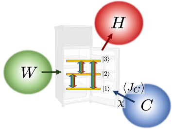
Figure 1: A scheme of the model refrigerator. The three-level system acts as a working material. Transitions between levels are induced by the heat baths. Unlike the optimal design Levy2012 ; Correa2014Nature , several reservoirs may simultaneously couple to the same transition.

Given this out-of-equilibrium, $N$-level, multi-bath model, our objective is to calculate the heat current extracted from the cold bath. We approach this challenge using a full-counting statistics (FCS) formalism EspositoReview ; hanggi-review ; bijay-wang-review . This tool provides the cumulant generating function (CGF) for heat exchange, thus fully characterizing energy exchange in steady state. The FCS treatment is appealing for several reasons: (i) It allows validation of the fluctuation symmetry, thus ensuring the thermodynamical consistency of approximate techniques. (ii) An FCS treatment automatically hands over the averaged current and high order cumulants. (iii) Practically, extending the Markovian population dynamics, Eq. (1), to report on the FCS of heat exchange is quite straightforward, as was exemplified in numerous studies EspositoReview ; Bijay-recon ; HavaNJP .

To derive the characteristic function for heat exchange, we follow the two-time measurement protocol EspositoReview and introduce a counting parameter $\chi$ which tracks thermal energy entering/leaving the cold reservoir. According to our sign convention, heat exchange (heat current) is positive when it flows towards the central system. In principle, one could keep track of energy transfer at each boundary with the system by introducing a counting parameter $\chi_{\mu}$ for each reservoir $\mu$ HavaNJP . However, to simplify our analysis we limit it to a single counting parameter.

In the MQME approach, the FCS is obtained by writing down the counting field-dependent quantum master equation, $\dot{p}(t,\chi)={\cal L(\chi)}\,p(t,\chi)$, with counting-field dependent Liouvillian and population. The microscopic derivation of this equation was detailed e.g. in Ref. HavaNJP , and exemplified in Appendix A and B for two- and three-level models, respectively.

The characteristic function for heat exchange is given by ${\cal Z}(t,\chi)=\langle I|p(t,\chi)\rangle$, where $\langle I|=(1,1,1,...)^{T}$ is the identity vector. The CGF for steady state heat exchange is obtained in the long time limit as

$${\cal G}(\chi)=\lim_{t\to\infty}\frac{1}{t}\ln{\cal Z}(t,\chi).$$ (2)

Differentiating this function $k$ times with respect to $(i\chi)$ brings the $k$th cumulant of the process. Specifically, the first cumulant is the energy current between the system and the reservoir where counting is performed,

$$\langle J\rangle=\frac{\partial\cal G}{\partial(i\chi)}\Big{|}_{\chi=0}.$$ (3)

The second cumulant is the noise of that current.

We obtain the CGF by diagonalizing ${\cal L}(\chi)$ and selecting the eigenvalue corresponding to the long-time limit. This is the eigenvalue with the smallest magnitude for its real part, $\lambda_{\textrm{min. real magnitude}}={\cal G}(\chi)$. Formally, we solve the eigenvalue problem by writing down the characteristic polynomial for the matrix ${\cal L}(\chi)$ in terms of its eigenvalues, $\lambda_{1,2,...,N}$,

$$\lambda_{i}^{N}+a_{1}(\chi)\,\lambda_{i}^{N-1}+...+a_{N-1}(\chi)\,\lambda_{i}+a_{N}(\chi)=0.$$

(4)

The coefficients $a_{j}(\chi)$ are functions of the counting parameter. In what follows, we distinguish between $a_{j}(\chi)$ and $a_{j}(0)$, which are the coefficients of the characteristic polynomials of ${\cal L}(\chi)$ and ${\cal L}(0)={\cal L}$, respectively. We now list several important properties of these elements.

The coefficients of the characteristic polynomial can be expressed in terms of the eigenvalues: $a_{j}(\chi)$ of $\lambda^{N-j}$ is given by the sum of all products of $j$ eigenvalues Brooks ,

$$a_{j}(\chi)=(-1)^{j}\sum_{{\rm all\,sets\,of\,}j\,\lambda^{\prime}s}\lambda_{k}\times\lambda_{p}\times...\times\lambda_{q}.$$ (5)

Specifically,

$$a_{1}(\chi) = -\operatorname{Tr}[{\cal L(\chi)}],$$

$$a_{N}(\chi) = (-1)^{N}\det[{\cal L}(\chi)],$$

$$a_{N}(0) = 0.$$ (6)

For the physical problems that we consider, the trace, $a_{1}(\chi)$ does not depend on the counting field, see Appendices A and B. As for the other coefficients, from the general rule we get e.g. that for a $3\times 3$ matrix, $a_{2}(\chi)=\lambda_{1}\lambda_{2}+\lambda_{1}\lambda_{3}+\lambda_{2}\lambda_{3}$. The last property in Eq. (6) stems from the fact that under our dynamics, the system reaches a unique steady state, thus ${\cal L}(0)$ must acquire a zero eigenvalue, which nullifies the determinant.

From the detailed balance condition it can be shown that the eigenvalues of ${\cal L}(0)$ must be real since the eigenvalue problem can be mapped to a real symmetric matrix. Furthermore, positive values for the eigenvalues are unphysical since that would lead to exponentially growing probabilities. ODEbook ; OQSbook . Therefore, the eigenvalues of the rate matrix ${\cal L}(0)$ are real, negative numbers. With that in mind, based on Eq. (5), we conclude that the coefficients $a_{1,2,...N}(0)$ must be positive. In particular, we later use the fact that $a_{N-1}(0)>0$.

II.2 Current and cooling condition

For an $N\times N$ problem, ${\mathcal{L}}(\chi)$ has $N$ eigenvalues, with ${\cal G}(\chi)$ as the eigenvalue with the smallest-magnitude real part. As discussed in Ref. Dvira2018 , the eigenvalue problem can be greatly simplified if we focus on the heat current only, Eq. (3): Because ${\cal G}(\chi=0)=0$, Eq. (4) can be truncated to first order in $\lambda$ – and would still solve exactly for the first cumulant. More generally, Eq. (4) can be truncated to the order of the desired cumulant.

Truncating the characteristic polynomial (4) to first order we get

$${\cal G}^{(1)}(\chi)=-\frac{a_{N}(\chi)}{a_{N-1}(\chi)}.$$ (7)

To obtain the heat current we differentiate Eq. (7) with respect to $(i\chi)$. Using $a_{N}(0)=0$, we arrive at

$$\langle J\rangle=\frac{\partial{\cal G}^{(1)}(\chi)}{\partial(i\chi)}\Big{|}_{\chi=0}=-\frac{1}{a_{N-1}(0)}\frac{\partial a_{N}(\chi)}{\partial(i\chi)}\Big{|}_{\chi=0}.$$ (8)

We recall that $a_{N}(\chi)=(-1)^{N}\textrm{det}\left[{\cal L}(\chi)\right]$. Applying Jacobi’s formula, which connects the derivative of the determinant to a trace relation, we get an analytic expression for the heat current, from the reservoir where counting is performed towards the quantum system,

$$\langle J\rangle=\frac{(-1)^{N+1}}{a_{N-1}(0)}\operatorname{Tr}\left[\textrm{adj}\left[{\cal L}(0)\right]\ \frac{\partial{\cal L}(\chi)}{\partial(i\chi)}\Bigg{|}_{\chi=0}\right].$$ (9)

Here, $\textrm{adj}\left[{\cal L}\right]$ is the adjugate matrix of the Liouvillian; the transpose of the cofactor matrix of ${\cal L}$. If counting is performed on the cold bath, Eq. (9) provides the cooling current $\langle J_{C}\rangle$. However, the equation can be readily applied to calculate other currents by assigning the counting parameter to the respective heat source.

We now write down a general condition on the cooling window. Since $a_{N-1}(0)>0$, cooling is achieved if

$$(-1)^{N+1}\operatorname{Tr}\left[\textrm{adj}\left[{\cal L}(0)\right]\ \frac{\partial{\cal L}(\chi)}{\partial(i\chi)}\Bigg{|}_{\chi=0}\right]>0.$$ (10)

Equations (9)-(10) are the main results of this paper. They offer the following benefits over standard calculations of the heat current commentJ :

(i) Equation (9) allows us to feasibly calculate heat currents analytically for systems described by the generic evolution, Eq. (1), without a prior knowledge of the steady state population. Similarly, the cooling condition (10) can be evaluated analytically to easily determine if a quantum system is suitable to act as a refrigerator.

(ii) In both Equations (9) and (10) only the diagonal elements of the matrix product are required to perform the trace operation. The matrix $\partial{\cal L}(\chi)/\partial(i\chi)|_{\chi=0}$ is sparse in typical models, thus drastically reducing the complexity of the calculation. Importantly, this matrix can be readily-intuitively constructed, and it does not require knowledge of the principles of the FCS formalism: As we illustrate in the Appendices, when calculating $\langle J_{\nu}\rangle$ the terms surviving in $\partial{\cal L}(\chi)/\partial(i\chi)|_{\chi=0}$ are energy transfer rates to/from the reservoir $\nu$ and the system.

(iii) Eq. (9) can be used to study heat exchange at each contact, thus providing the cooling coefficient of performance, that is the ratio of cooling current to input power extracted from the work reservoir.

(iv) Our derivation for the cooling current does not discriminate between different sources of irreversibility: whether these are due to the competition between different cooling pathways (“internal dissipation”) or due to heat leaks with multiple reservoirs coupled to the driving (work) transition.

(v) Our derivation does not rely on the additivity of the total Liouvillian with the different baths. Therefore, expressions (9)-(10) can be applied to more general setups, such as the non-additive system-bath models discussed in Ref. HavaNJP .

Appendix A exemplifies the evaluation of the heat current in a two-level two-bath setup. In Appendix B, we construct three-level three-bath models and illustrate the calculation of the cooling current and cooling condition in ideal and non-ideal QARs.

II.3 Noise power

It is possible to obtain the noise power of a specific current, $\langle S\rangle=\frac{\partial^{2}\cal G}{\partial(i\chi)^{2}}\Big{|}_{\chi=0}$ by following a similar procedure to the calculation of the heat current. To achieve that, we use a characteristic polynomial truncated to second order in $\lambda$, $a_{N-2}(\chi)\lambda^{2}+a_{N-1}(\chi)\lambda+a_{N}(\chi)=0$, which yields the CGF,

$${\cal G}^{(2)}(\chi)=\frac{-a_{N-1}(\chi)+\sqrt{a_{N-1}(\chi)^{2}-4a_{N}(\chi)a_{N-2}(\chi)}}{2a_{N-2}(\chi)}.$$

The resulting noise expression [after a second derivative in ($i\chi$)] is cumbersome. Therefore, we only consider classes of models for which both $a_{N-1}(\chi)$ and $a_{N-2}(\chi)$ do not depend on the counting parameter. This is the case, for example, for a three level system if we further assume that the cold bath is coupled to a specific transition that no other bath is coupled to commentN3 . Under this approximation, the noise can be received via

$$\langle S\rangle=\frac{(-1)^{N+1}}{a_{N-1}(0)} \operatorname{Tr} \left[\frac{\partial\textrm{adj}[{\cal L(\chi)}]}{\partial(i\chi)}\frac{\partial{\cal L}}{\partial(i\chi)}+\textrm{adj}[{\cal L}(0)]\frac{\partial^{2}{\cal L}}{\partial(i\chi)^{2}}\right]_{\chi=0}$$ (12)

$$- 2\left(\frac{a_{N-2}(0)}{a_{N-1}(0)}\right)\langle J\rangle^{2}.$$

For a given device setup, the noise could be minimized with respect to tunable parameters to determine the fundamental limit of noise reduction. While this expression seems cumbersome, the extreme sparsity of the differentiated Liouvillian matrices drastically simplifies calculations.

III Case study: Three-level QAR with competing cycles and leaks

A QAR is a continuous-cycle heat machine, which operates without external driving. It extracts energy from a cold ($C$) reservoir assisted by heat supplied from a so-called work reservoir ($W$), and it dumps the heat into a hot reservoir ($H$). The simplest version of such a device, the three-level quantum absorption refrigerator Scovil-Schluz-Dubois , has been explored in detail in the weak system-bath coupling limit Kosloff2001 ; Skrzypczyk2010 .

We exemplify the analytic results derived in Sec. (II) on a general, non-ideal three-level QAR. The setup includes three levels, $\ket{1}$, $\ket{2}$, and $\ket{3}$. Transitions between states $\ket{i}$ and $\ket{j}$ are induced by three heat baths, with $\beta_{C}>\beta_{H}>\beta_{W}$; $\beta_{\mu}$ is the inverse temperature of the $\mu$ bath. The Hamiltonian of the setup is given by,

$$\hat{H}=\sum_{j=1}^{3}E_{j}\ket{j}\bra{j}+\sum_{\begin{subarray}{c}\mu=C,H,W\end{subarray}}\sum_{k}\omega_{\mu,k}\,\hat{a}^{\dagger}_{\mu,k}\hat{a}_{\mu,k}$$

$$+\sum_{\begin{subarray}{c}\mu=C,H,W\end{subarray}}\sum_{\begin{subarray}{c}j>i\end{subarray}}\hat{B}_{ij}^{\mu}(\ket{i}\bra{j}+h.c.)$$

(13)

Here, $\hat{a}^{\dagger}_{\mu,k}$ ($\hat{a}_{\mu,k}$) is a bosonic creation (annihilation) operator of mode $k$ in the $\mu$ bath. $\hat{B}_{ij}^{\mu}=\sum_{k}u_{ij}^{\mu,k}\left(\hat{a}^{\dagger}_{\mu,k}+\hat{a}_{\mu,k}\right)$ is a bath operator that couples to the $i\leftrightarrow j$ transition with energy $u_{ij}^{\mu}$, which is assumed to be a real number.

The Hamiltonian (13) is a general version of the ideal 3-level quantum absorption refrigerator, in which only the $u_{12}^{C}$, $u_{23}^{W}$ and $u_{13}^{H}$ transition elements are nonzero; this scenario is ‘ideal’ because tuning the system’s parameters (energy levels) can achieve the Carnot cooling limit, see Appendix B and e.g. Refs. Correa2014Nature ; Dvira2018 .

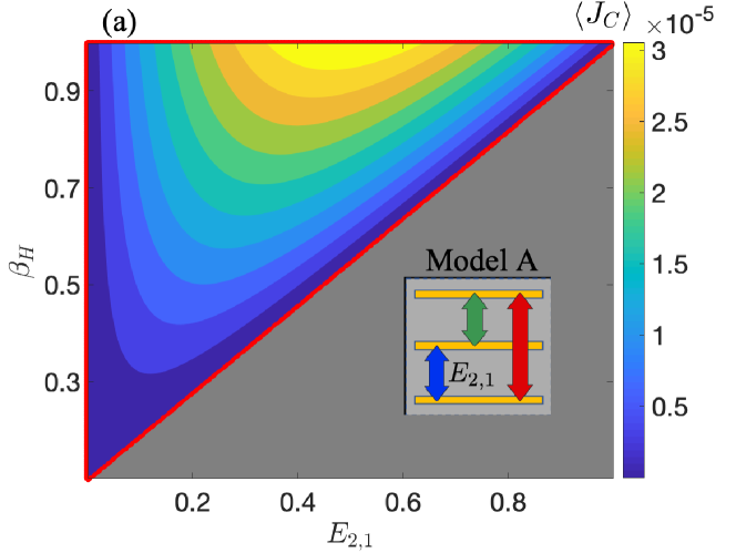
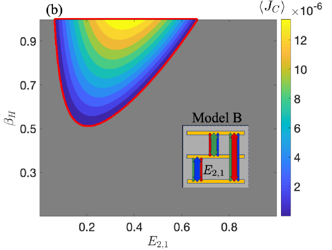
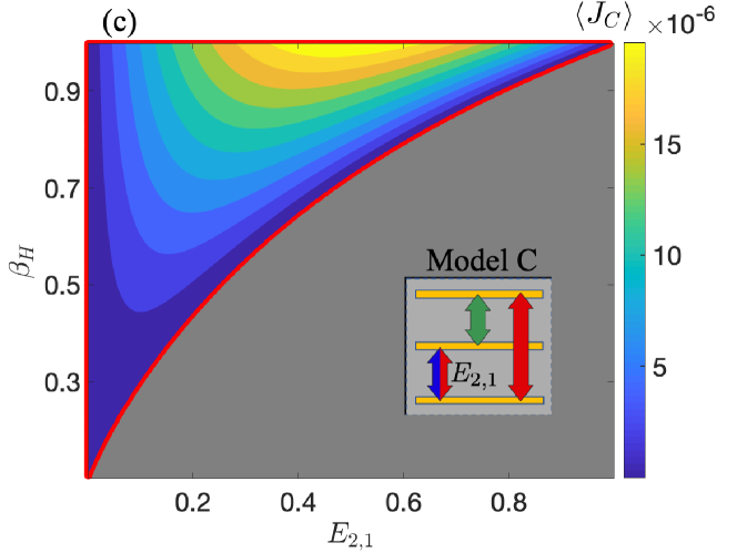
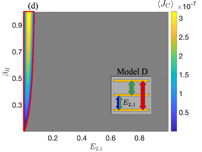
Figure 2: Cooling currents of three-level QAR as a function of energy spacing $E_{2,1}$ and the inverse temperature of the hot reservoir, $\beta_{H}$. The colored region corresponds to a positive current: heat extracted from the cold bath. The red outline encloses the region where Eq. (10) predicts cooling to occur. Parameters are $E_{3,1}=1$, $\beta_{C}=1$, $\beta_{W}=0.1$, $\omega_{C}=10$, $\gamma=0.001$ and $\tilde{\gamma}=\gamma/50$. (a) Model A. Ideal QAR setup, $\gamma=\gamma^{C}_{12}=\gamma^{H}_{13}=\gamma^{W}_{23}$. (b) Model B. QAR with dominant transitions, $\gamma=\gamma^{C}_{12}=\gamma^{H}_{13}=\gamma^{W}_{23}$ and additional weaker transitions, $\tilde{\gamma}=\gamma^{C,W}_{13}=\gamma^{C,H}_{23}=\gamma^{W,H}_{12}$. (c) Model C. QAR with heat leaks from the hot bath, $\gamma=\gamma^{C,H}_{12}=\gamma^{H}_{13}=\gamma^{W}_{13}$. (d) Model D. QAR with heat leaks from the work bath, $\gamma=\gamma^{C,W}_{12}=\gamma^{H}_{13}=\gamma^{W}_{23}$. Coupling coefficients that are not indicated are null.

In what follows, we study the cooling performance of non-ideal setups. Specifically, in our work, the term ‘heat leaks’ refers to having several baths coupled to the same transition. This leads to a competition between the different baths, to either excite or relax population. Internal dissipation arrises when cooling can be achieved by more than one cycle Correa2015PRE .

We can feasibly predict the parameters for the cooling window by writing down the Liouvillian ${\cal L}(\chi)={\cal L}_{C}(\chi)+{\cal L}_{W}+{\cal L}_{H}$. For harmonic baths and bilinear system-bath couplings the Liouvillians are made from the rate constants,

$$k_{i\to j}^{\mu}=\begin{cases}\Gamma^{\mu}_{ij}(E_{j,i})n_{\mu}(E_{j,i})&E_{j}>E_{i}\\ \Gamma^{\mu}_{ij}(E_{i,j})[n_{\mu}(E_{i,j})+1]&E_{j}<E_{i}.\end{cases}$$ (14)

Here, $n_{\mu}(\omega)=[e^{\beta_{\mu}\omega}-1]^{-1}$ is the Bose-Einstein occupation function. $\Gamma^{\mu}_{ij}(\omega)=2\pi\sum_{k}(u_{ij}^{\mu,k})^{2}\delta(\omega-\omega_{\mu,k})$ is the spectral density function of the baths, $E_{i,j}=E_{i}-E_{j}$. Specifically, we employ an ohmic model, $\Gamma^{\mu}_{ij}(\omega)=\gamma_{ij}^{\mu}\omega e^{-|\omega|/\omega_{c}}$ with $\gamma$ as a dimensionless coupling parameter and $\omega_{c}$ the cutoff frequency, assumed to be high. Since we study the problem in the weak-coupling limit, the full functional form of the spectral function carries no impact on the cooling current; only the value in resonance with the system’s transitions is used in calculations.

We examine different configurations of the QAR model in the four panels of Fig. (2). In each case, we indicate schematically the allowed transitions as activated by the different baths using colored arrows: blue for the $C$ bath, red for $H$, and green for $W$. The relative width of the arrows indicate the relative strength of that bath-induced transition. The red curve encloses the region where cooling is predicted according to Eq. (10), and the contours show the positive cooling current calculated numerically. For visibility, negative current (heat flow directed towards the cold bath) is not presented (gray region). As can be seen, the cooling condition (red curve) perfectly predicts the cooling window for each of the QAR setups.

Our analysis demonstrates that the current at the cold contact can be generally written as

$$\langle J_{C}\rangle=\sum_{i>j}F_{cyc}^{i,j}+\sum_{\mu,i>j}F_{leak,\mu}^{i,j}.$$ (15)

Here, $F_{cyc}^{i,j}$ identifies a circuit that can realize a QAR with the cold bath coupled to the $i\leftrightarrow j$ transition and the work and hot baths completing a cycle, e.g. $i\xrightarrow{C}j\xrightarrow{W}j^{\prime}\xrightarrow{H}i$, and the reversed process. ‘Cycle’ contributions must involve the three baths. The second term, $F_{leak,\mu}^{i,j}$, is always negative. It comprises heat leaks from the $\mu$ bath to the cold bath when both reservoirs are coupled to the $i\leftrightarrow j$ transition. Thus, leak terms involve two reservoirs, either $H$ or $W$, and $C$. This classification (see Appendix B) agrees with AlonsoNJP17 . We now use Eq. (15) to explain the results of Fig. 2.

Model A. The ideal QAR setup is constructed by taking nonzero values for $\gamma_{12}^{C}$, $\gamma_{23}^{W}$, $\gamma_{13}^{H}$; all other couplings are null. As we show in panel a, this setup achieves the widest cooling window and the most substantial cooling current. We note that there is an optimal level spacing $E_{2,1}$ for maximizing the cooling current, which depends on the temperature of the cold bath. This setup is termed ‘ideal’ since it can achieve the Carnot bound. Increasing $\beta_{H}$ (decreasing $T_{H}$) is beneficial for cooling: When the temperature gradient between $H$ and $C$ is reduced, heat flow from $H$ to $C$ is minimized. In Appendix B we use Eq. (10) and derive the cooling condition, $F_{cyc}^{2,1}>0$, or explicitly

$$F_{cyc}^{2,1} = E_{2,1}k_{3\to 1}^{H}k_{3\to 2}^{W}k_{2\to 1}^{C}$$ (16)

$$\times \left(e^{-\beta_{W}E_{3,2}}e^{-\beta_{C}E_{2,1}}-e^{-\beta_{H}E_{3,1}}\right)>0.$$

It agrees with previous studies, see e.g. Correa2014Nature . Next, the ideal configuration is compromised by including additional couplings, resulting in heat leaks.

Model B. Here we distinguish between ‘dominant’ couplings, which reproduce the ideal setup, $\gamma=\gamma_{12}^{C}=\gamma_{23}^{W}=\gamma_{13}^{H}$, and secondary-weaker couplings, which lead to heat leakage and competition between cycles, $\tilde{\gamma}=\gamma_{13}^{C,W}=\gamma_{23}^{C,H}=\gamma_{12}^{H,W}$, with $\tilde{\gamma}\ll\gamma$. Results are presented in panel b. We find that the cooling function disappears for small $E_{2,1}$, but it survives in the intermediate $E_{2,1}\sim E_{3,2}$ regime. We can rationalize our observations as follows (Appendix B): While heat directly leaks to the cold bath from both the hot and work reservoirs, we may extract energy from the cold bath using the different cycles. We note that $F_{cyc}^{3,1}$ is always negative thus we are left with two cycles, $F_{cyc}^{2,1}$ and $F_{cyc}^{3,2}$. The cooling condition for cycle $F_{cyc}^{2,1}$ is

$$\frac{E_{2,1}}{E_{3,1}}\leq\frac{\beta_{H}-\beta_{W}}{\beta_{C}-\beta_{W}}.$$ (17)

In contrast, cooling via the cycle $F_{cyc}^{3,2}$ is achieved if we satisfy

$$\frac{E_{2,1}}{E_{3,1}}\geq\frac{\beta_{C}-\beta_{H}}{\beta_{C}-\beta_{W}}.$$ (18)

The two cycles have conflicting requirements on the energy gap $E_{2,1}$, thus cooling is not achievable for either small or large $E_{2,1}$, when one of the cycles delivers heat into the cold bath. Furthermore, heat leaks and the non-cooling $F_{cyc}^{3,1}$ cycle suppress the cooling current for both small and large $E_{2,1}$ spacing.

Model C. In this model (panel c) the hot bath directly competes with the cold bath on the cooling performance. As we show in Appendix B, the cooling condition of the setup can be compactly written as

$$F_{cyc}^{2,1}+F_{leak,H}^{2,1}>0,$$ (19)

with $F_{leak,H}^{2,1}\propto\left(e^{-\beta_{C}E_{2,1}}-e^{-\beta_{H}E_{2,1}}\right)$, which is negative. Therefore, the extracted current is smaller than in Model A, and the cooling condition is more difficult to satisfy, resulting in a more limited window of operation. Specifically, beyond a certain value for $E_{2,1}$, the cooling function is lost since the heat leak term takes over.

Model D. This setup (panel d) is similar to Model C, but with the work bath directly competing with the cold bath. A cooling condition, analogous to Eq. (19), can be written. However, given that $\beta_{W}\ll\beta_{C}$, the cooling performance is significantly reduced, and it survives only for very small energy splitting, $E_{2,1}$.

The secular approximation breaks down when two quasidegenerate levels are coupled to a third level, with the same bath responsible for transitions between the ground and excited states. In Fig. 2, the energy level $E_{2}$ is allowed to move in the full range between $E_{1}$ and $E_{3}$, thus reaching degeneracy in the extreme limits. However, our analysis and conclusions do not pertain to these special limits. Specifically, in panel b the region of no-cooling at small $E_{2,1}$ is controlled by $\tilde{\gamma}$, and not by coherent effects. In panel d, our main observation is the suppression of the central cooling region (when $E_{2}$ is set about halfway in the $E_{3,1}$ gap). This suppression is controlled by a leakage process from the work bath.

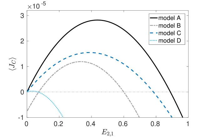
Figure 3: Heat current $\langle J_{C}\rangle$ with varying level spacing, $E_{2,1}$. The different curves correspond to the QAR results as presented in Fig. 2 for $\beta_{H}=0.9$.

In Fig. 3 we display examples based on Fig. 2 and highlight the different magnitudes of the cooling currents. Because $T_{H}$ is close to $T_{C}$, the cooling behavior is moderately-negatively impacted in models B and C relative to model A. In contrast, heat leaks from the work to the cold reservoir (model D) dramatically lessen both the cooling window and the cooling current.

IV Summary

We derived a cooling condition for a multilevel quantum absorption refrigerator described at the level of a Markovian quantum master equation. The obtained cooling condition is given in terms of the generator of the dynamics, and it provides analytical insight to the machine operation. It allows us to determine the effect of heat leaks and competing cycles in the setup, and feasibly identify the parameter space that achieves the desired function. We further obtained a closed-form expression for the currents (cooling or input power) in the model, and described the calculation of the current noise. We expect this work to assist in the quest to realize QARs; a realistic device evidently suffers from leakage and internal dissipation processes. While we exemplified our results on a three-level QAR, the formalism holds for a general $N$-level system, with the heat current combining cycles and leaks as in Eq. (15).

Steady-state coherences arise in $V$ and $\Lambda$-type level structure when nonequilibrium baths are coupled to the energy degenerate transitions Michael2018 . The impact of such coherences on the cooling current can be studied numerically with a non-secular MQME Michael2018 ; Noise2018 ; Pet ; Zambrini . A recent study showed that under some assumptions, quantum coherent devices can be mapped onto a “classical emulator” that reproduces the same thermodynamic performance in the long time limit Correa19PRE , where our formalism could be applied. Achieving a compact, feasible cooling condition in cases that cannot be described by a classical-incoherent emulator is left for future work.

Appendix A: The nonequilibrium spin-boson model

We show that Eqs. (9) and (12) reproduce known results for the heat current and its noise in the nonequilibrium spin boson model ($N=2$), displayed in Fig. (4). The Hamiltonian of the model is

$$\hat{H}=\frac{\omega_{0}}{2}\hat{\sigma}_{z}+\sum_{\begin{subarray}{c}\mu,k\end{subarray}}\omega_{\mu,k}\,\hat{a}^{\dagger}_{\mu,k}\hat{a}_{\mu,k},+\hat{\sigma}_{x}\sum_{\mu}\hat{B}^{\mu},$$ (A1)

where $\hat{B}^{\mu}=\sum u^{\mu,k}(\hat{a}_{\mu,k}^{\dagger}+\hat{a}_{\mu,k})$. The counting field dependent MQME reads ${\dot{p}(t,\chi)}={\cal L}(\chi){p(t,\chi)}$ with the Liouvillian rate matrix HavaNJP ,

$${\cal L}(\chi)=\begin{pmatrix}-k_{1\to 2}^{C}-k_{1\to 2}^{H}&k_{2\to 1}^{C}e^{-i\chi\omega_{0}}+k_{2\to 1}^{H}\\ k_{1\to 2}^{C}e^{i\chi\omega_{0}}+k_{1\to 2}^{H}&-k_{2\to 1}^{C}-k_{2\to 1}^{H}\end{pmatrix}$$

In this equation, rate constants describing heat exchange with the cold bath are decorated by the counting fields. The ‘bare’ rate constants are $k_{1\to 2}^{\mu}=\int_{-\infty}^{\infty}dt\,e^{-i\omega_{0}t}\langle\hat{B}^{\mu}(t)\hat{B}^{\mu}(0)\rangle$, and the detailed balance condition enforces $k_{1\to 2}^{\mu}=e^{-\beta_{\mu}\omega_{0}}k_{2\to 1}^{\mu}$. To use equation (9) we calculate the derivative,

$$\frac{\partial{\cal L}(\chi)}{\partial(i\chi)}\Bigg{|}_{\chi=0}=\begin{pmatrix}0&-\omega_{0}\,k_{2\to 1}^{C}\\ \omega_{0}\,k_{1\to 2}^{C}&0\end{pmatrix}.$$

We note the natural form of this matrix, allowing us to create it intuitively: It includes heat transfer rates to/from the cold bath with the appropriate sign convention.

Using Eq. (9) we can now determine the current from the $C$ bath,

$$\langle J_{C}\rangle=\frac{-1}{a_{1}(0)}\operatorname{Tr}\left[\begin{pmatrix}C_{11}&C_{21}\\ C_{12}&C_{22}\end{pmatrix}\begin{pmatrix}0&-\omega_{0}\,k_{2\to 1}^{C}\\ \omega_{0}\,k_{1\to 2}^{C}&0\end{pmatrix}\right]$$

The matrix filled with the cofactor terms $C_{ij}$ is the adjugate matrix, $\textrm{adj}[{\cal L}(0)]$. $a_{1}(0)$ is the coefficient of $\lambda$ in the characteristic polynomial, Eq. (4). Simplifying, and marking only the relevant terms, while using the fact that $a_{1}(0)=\operatorname{Tr}\left[{\cal L}(0)\right]$, we get

$$\langle J_{C}\rangle=\frac{-1}{\operatorname{Tr}\left[{\cal L}(0)\right]}\operatorname{Tr}\left[\begin{pmatrix}C_{21}\omega_{0}\,k_{1\to 2}^{C}&...\\ ...&-C_{12}\omega_{0}\,k_{2\to 1}^{C}\end{pmatrix}\right].$$

(A2)

We need only solve for $C_{12}$ and $C_{21}$ from the adjugate matrix. Trivially, $C_{12}=-[\mathcal{L}(0)]_{2,1}=(k_{1\to 2}^{C}+k_{1\to 2}^{H})$ and $C_{21}=-[\mathcal{L}(0)]_{1,2}=(k_{2\to 1}^{C}+k_{2\to 1}^{H})$, which results in

$$\langle J_{C}\rangle=\frac{\omega_{0}\left[k_{1\to 2}^{H}k_{2\to 1}^{C}-k_{2\to 1}^{H}k_{1\to 2}^{C}\right]}{k_{1\to 2}^{C}+k_{1\to 2}^{H}+k_{2\to 1}^{C}+k_{2\to 1}^{H}}.$$ (A3)

Using the harmonic bath model and bilinear system-bath coupling the rate constants are $k_{2\to 1}^{\mu}=\Gamma_{\mu}(\omega_{0})[n_{\mu}(\omega_{0})+1]$ and $k_{1\to 2}^{\mu}=\Gamma_{\mu}(\omega_{0})n_{\mu}(\omega_{0})$, therefore

$$\langle J_{C}\rangle=\frac{\omega_{0}\Gamma_{C}(\omega_{0})\Gamma_{H}(\omega_{0})\left[n_{C}(\omega_{0})-n_{H}(\omega_{0})\right]}{\Gamma_{C}(\omega_{0})[1+2n_{C}(\omega_{0})]+\Gamma_{H}(\omega_{0})[1+2n_{H}(\omega_{0})]}.$$

Here, $\Gamma_{\mu}(\omega_{0})=2\pi\sum_{k}(u^{\mu,k})^{2}\delta(\omega_{0}-\omega_{\mu,k})$ is the spectral density of the $\mu$ bath evaluated at $\omega_{0}$ and $n_{\mu}(\omega_{0})=(e^{\beta_{\mu}\omega_{0}}-1)^{-1}$ is the Bose-Einstein distribution function.

Equation (Appendix A: The nonequilibrium spin-boson model) agrees with previous studies Segal04 ; Segal06 ; Yelena10 . However, the present evaluation, which is based on Eq. (A2) is almost trivial compared to the standard approach, which requires one to solve the equation of motion for the population in steady state, then substitute the population in the expression for the current.

Beyond the current, we follow the procedure for calculating the current noise using Eq. (12). In this case we need to examine two matrices $\partial^{2}{\cal L(\chi)}/\partial(i\chi)^{2}$ and $\partial\textrm{adj}\left[{\cal L}(\chi)\right]/\partial(i\chi)$. The former is easy to calculate,

$$\frac{\partial^{2}{\cal L}(\chi)}{\partial(i\chi)^{2}}\Bigg{|}_{\chi=0}=\begin{pmatrix}0&\omega_{0}^{2}\,k_{2\to 1}^{C}\\ \omega_{0}^{2}\,k_{1\to 2}^{C}&0\end{pmatrix}.$$

As for the latter, again, we only need to study two elements,

$$\frac{\partial C_{21}}{\partial(i\chi)}=\omega_{0}k^{C}_{2\to 1},\,\,\,\,\,\,\,\,\,\,\frac{\partial C_{12}}{\partial(i\chi)}=-\omega_{0}k^{C}_{1\to 2}.$$

Altogether, we get

$$\langle S_{C}\rangle = \frac{\omega_{0}^{2}\left[k_{2\to 1}^{H}k_{1\to 2}^{C}+k_{1\to 2}^{H}k_{2\to 1}^{C}\right]-2\langle J_{C}\rangle^{2}}{k_{1\to 2}^{C}+k_{1\to 2}^{H}+k_{2\to 1}^{C}+k_{2\to 1}^{H}},$$

which reduces to the known result Yelena10

$$\langle S_{C}\rangle=\frac{\omega_{0}^{2}\,\Gamma_{C}\Gamma_{H}\left[(1+n_{C})n_{H}+(1+n_{H})n_{C}\right]-2\langle J_{C}\rangle^{2}}{\Gamma_{C}(1+2n_{C})+\Gamma_{H}(1+2n_{H})}.$$

Here, $\Gamma_{\mu}$ and $n_{\mu}$ are evaluated at the frequency of the spin, $\omega_{0}$.

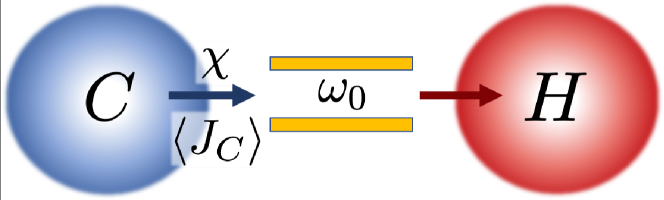
Figure 4: Scheme of the nonequilibrium two-level system. By introducing a counting parameter on the cold bath, we calculate the heat current extracted from this bath to the system, which is negative in this two-terminal problem.

Appendix B: Ideal and non-ideal three-level QAR

We describe here the calculation of the cooling window in the different 3-level models presented in the four panels of Fig. 2.

IV.1 Ideal QAR: Model A

We exemplify our procedure to obtain a cooling condition [Eq. (10)] on the canonical three-level quantum absorption refrigerator with ‘ideal’ coupling operator. The Hamiltonian of the model reads

$$\hat{H} = \sum_{j=1}^{3}E_{j}\ket{j}\bra{j}+\sum_{\begin{subarray}{c}\mu,k\end{subarray}}\omega_{\mu,k}\,\hat{a}^{\dagger}_{\mu,k}\hat{a}_{\mu,k}$$ (B1)

$$+ \hat{B}^{C}_{12}\left(\ket{1}\bra{2}+\ket{2}\bra{1}\right)+\hat{B}^{H}_{13}\left(\ket{1}\bra{3}+\ket{3}\bra{1}\right)$$

$$+ \hat{B}^{W}_{23}\left(\ket{2}\bra{3}+\ket{3}\bra{2}\right).$$

where $\hat{B}^{\mu}_{ij}=\sum_{k}u^{\mu,k}_{ij}(\hat{a}^{\dagger}_{\mu,k}+a_{\mu,k})$ is an operator of the $\mu$ heat bath. The equations of motion for the populations are given by $\dot{p}(t)={\cal L}(0)\,p(t)$ with the population vector $p(t)=(p_{1}(t),p_{2}(t),p_{3}(t))^{T}$ and the Liouvillian

$${\cal L}(0)=\begin{pmatrix}-k_{1\to 2}^{C}-k_{1\to 3}^{H}&k_{2\to 1}^{C}&k_{3\to 1}^{H}\\ k_{1\to 2}^{C}&-k_{2\to 1}^{C}-k_{2\to 3}^{W}&k_{3\to 2}^{W}\\ k_{1\to 3}^{H}&k_{2\to 3}^{W}&-k_{3\to 1}^{H}-k_{3\to 2}^{W}\end{pmatrix}$$

The rate constants are

$$k^{C}_{1\to 2} = \Gamma_{C}(E_{2,1})n_{C}(E_{2,1}),$$

$$k_{1\to 3}^{H} = \Gamma_{H}(E_{3,1})n_{H}(E_{3,1}),$$

$$k_{2\to 3}^{W} = \Gamma_{W}(E_{3,2})n_{W}(E_{3,2}).$$ (B3)

The detailed balance relation dictates the rate constants of reversed processes, e.g., $k_{2\to 1}^{C}=\Gamma_{C}(E_{2,1})\left[n_{C}(E_{2,1})+1\right]$. The system-bath coupling constants (hybridization) are $\Gamma_{\mu}(\omega)=2\pi\sum_{k}(u_{ij}^{\mu,k})^{2}\delta(\omega_{\mu,k}-\omega)$. The Bose-Einstein occupation factors are $n_{\mu}(\omega)=[e^{\beta_{\mu}\omega}-1]^{-1}$, given in terms of the inverse temperature $\beta_{\mu}=1/(k_{B}T_{\mu})$. In the weak-coupling approximation employed here, only resonant processes are allowed.

The cumulant generating function of the model can be derived by following a rigorous procedure EspositoReview ; HavaNJP . Here, we employ a classical, intuitive derivation of the FCS; it agrees with the rigorous method under the weak-coupling, Markovian and secular approximations HavaNJP . We begin by defining $\mathcal{P}_{t}(j,nE_{2,1})$ as the probability that by the (long) time $t$, the thermal energy $nE_{2,1}$ had been absorbed by the system (transferred from the cold bath), and the system occupies the state $j=1,2,3$. Note that, for simplicity, we count energy exchanged with the cold bath only. Here, $n$ is an integer since under the weak coupling approximation heat is transferred into and out of the system in discrete quanta, in resonance with system’s level spacing. We readily write down an equation of motion for $\mathcal{P}_{t}(j,nE_{2,1})$ EspositoReview ; Renjie ; Yelena10 ,

$$\dot{\mathcal{P}}_{t}(1,nE_{2,1}) = -\mathcal{P}_{t}(1,nE_{2,1})(k_{1\rightarrow 2}^{C}+k_{1\rightarrow 3}^{H})+\mathcal{P}_{t}(2,(n+1)E_{2,1})k_{2\rightarrow 1}^{C}+\mathcal{P}_{t}(3,nE_{2,1})k_{3\rightarrow 1}^{H},$$

$$\dot{\mathcal{P}}_{t}(2,nE_{2,1}) = -\mathcal{P}_{t}(2,nE_{2,1})(k_{2\rightarrow 1}^{C}+k_{2\rightarrow 3}^{W})+\mathcal{P}_{t}(1,(n-1)E_{2,1})k_{1\rightarrow 2}^{C}+\mathcal{P}_{t}(3,nE_{2,1})k_{3\rightarrow 2}^{W},$$

$$\dot{\mathcal{P}}_{t}(3,nE_{2,1}) = -\mathcal{P}_{t}(3,nE_{2,1})(k_{3\rightarrow 1}^{H}+k_{3\rightarrow 2}^{W})+\mathcal{P}_{t}(2,nE_{2,1})k_{2\rightarrow 3}^{W}+\mathcal{P}_{t}(1,nE_{2,1})k_{1\rightarrow 3}^{H}.$$ (B4)

The equation is Fourier-transformed with the counting field $\chi$, and we define the counting field dependent population

$$|p(\chi,t)\rangle=\begin{pmatrix}\sum_{n=-\infty}^{\infty}\mathcal{P}_{t}(1,nE_{2,1})e^{inE_{2,1}\chi}\\ \sum_{n=-\infty}^{\infty}\mathcal{P}_{t}(2,nE_{2,1})e^{inE_{2,1}\chi}\\ \sum_{n=-\infty}^{\infty}\mathcal{P}_{t}(3,nE_{2,1})e^{inE_{2,1}\chi}\end{pmatrix}$$

(B5)

Note: the sign convention in the Fourier transform dictates the sign convention for the heat current, with positive current corresponding to heat absorbed by the system. Using Eq. (B4), we write down the set of differential equations,

$$\dot{p}(\chi,t)={\mathcal{L}}(\chi)p(\chi,t)$$ (B6)

with the rate matrix (Liouvillian)

$${\cal L}(\chi)=\begin{pmatrix}-k_{1\to 2}^{C}-k_{1\to 3}^{H}&k_{2\to 1}^{C}e^{-i\chi E_{2,1}}&k_{3\to 1}^{H}\\ k_{1\to 2}^{C}e^{i\chi E_{2,1}}&-k_{2\to 1}^{C}-k_{2\to 3}^{W}&k_{3\to 2}^{W}\\ k_{1\to 3}^{H}&k_{2\to 3}^{W}&-k_{3\to 1}^{H}-k_{3\to 2}^{W}\end{pmatrix}.$$

The characteristic function is given by ${\mathcal{Z}}(\chi,t)=\langle I|p(\chi,t)\rangle$ with the identity vector $\langle I|$. We now employ Eq. (10) to determine the cooling condition for the setup. We calculate the derivatives of the elements in ${\mathcal{L}}(\chi)$,

$$\frac{\partial{\cal L}(\chi)}{\partial(i\chi)}\Bigg{|}_{\chi=0}=\begin{pmatrix}0&-E_{2,1}\,k_{2\to 1}^{C}&0\\ E_{2,1}\,k_{1\to 2}^{C}&0&0\\ 0&0&0\end{pmatrix}.$$

(B8)

Again, we remark on the intuitive form of this matrix, pointing to the cooling processes. It can be constructed without prior knowledge of the FCS method. The cooling condition is

$$\operatorname{Tr}\left[\begin{pmatrix}C_{11}&C_{21}&C_{31}\\ C_{12}&C_{22}&C_{32}\\ C_{13}&C_{23}&C_{33}\end{pmatrix}\begin{pmatrix}0&-E_{2,1}\,k_{2\to 1}^{C}&0\\ E_{2,1}\,k_{1\to 2}^{C}&0&0\\ 0&0&0\end{pmatrix}\right]>0,$$

The matrix filled with the cofactors $C_{ij}$ is the adjugate matrix of the Liouvillian, ${\mathcal{L}}(0)$. This cooling condition condenses into

$$C_{21}e^{-\beta_{C}E_{2,1}}-C_{12}>0.$$ (B9)

If we interpret the cofactors as effective population, $C_{21}\leftrightarrow p_{1}$ and $C_{12}\leftrightarrow p_{2}$, we rationalize the cooling condition as (nonequilibrium) deviations from the detailed balance relation. We now evaluate the cofactors,

$$C_{21} = k^{C}_{2\to 1}k^{W}_{3\to 2}+k^{C}_{2\to 1}k^{H}_{3\to 1}+k^{H}_{3\to 1}k^{W}_{3\to 2}e^{-\beta_{W}E_{3,2}},$$

$$C_{12} = k^{C}_{2\to 1}k^{W}_{3\to 2}e^{-\beta_{C}E_{2,1}}+k^{C}_{2\to 1}k^{H}_{3\to 1}e^{-\beta_{C}E_{2,1}}$$ (B10)

$$+ k^{H}_{3\to 1}k^{W}_{3\to 2}e^{-\beta_{H}E_{3,1}},$$

and substitute them in Eq. (B9). Altogether we get

$$e^{-\beta_{W}E_{3,2}}e^{-\beta_{C}E_{2,1}}-e^{-\beta_{H}E_{3,1}}>0.$$ (B11)

This inequality can be simplified to arrive at the well-known cooling condition

$$\frac{E_{2,1}}{E_{3,1}}<\frac{\beta_{H}-\beta_{W}}{\beta_{C}-\beta_{W}}.$$ (B12)

The formalism provides the cooling current, and following similar steps, we get the heat absorbed from the work reservoir as well, thus the cooling coefficient of performance, $\eta\equiv\langle J_{C}\rangle/\langle J_{W}\rangle=E_{2,1}/E_{3,2}$. Combining this with Eq. (B12) we conclude that $\eta\leq\eta_{c}$ with the Carnot cooling efficiency $\eta_{c}=(\beta_{H}-\beta_{W})/(\beta_{C}-\beta_{H})$. Since one can tune parameters to reach the maximal cooling performance, we refer to this model as ‘ideal’. This concludes the derivation of the cooling window for Model A presented in Fig. 2(a).

IV.2 Non-ideal QAR: Model B

We analyze here Model B, as described and presented in Fig. 2(b). The Hamiltonian is given by

$$\hat{H} = \sum_{j=1}^{3}E_{j}\ket{j}\bra{j}+\sum_{\begin{subarray}{c}\mu,k\end{subarray}}\omega_{\mu,k}\,\hat{a}^{\dagger}_{\mu,k}\hat{a}_{\mu,k}$$ (B13)

$$+ \sum_{\mu\in C,W,H}\sum_{i>j}\hat{B}^{\mu}_{ij}(\ket{i}\bra{j}+\ket{j}\bra{i}).$$

In this model, each transition in the system is coupled to the three reservoirs, albeit we distinguish between ‘dominant’ couplings as in the ideal QAR model, and secondary (weaker) couplings. Following the standard steps as performed for the ideal model, we arrive at an equation of motion for the counting field-dependent population, $\dot{p}(\chi,t)={\mathcal{L}}(\chi)p(\chi,t)$ with the Liouvillian

$${\cal L}(\chi)=\begin{pmatrix}-\sum_{\mu=C,H,W}(k_{1\to 2}^{\mu}+k_{1\to 3}^{\mu})&k_{2\to 1}^{C}e^{-i\chi E_{2,1}}+k_{2\to 1}^{H}+k_{2\to 1}^{W}&k_{3\to 1}^{C}e^{-i\chi E_{3,1}}+k_{3\to 1}^{H}+k_{3\to 1}^{W}\\ k_{1\to 2}^{C}e^{i\chi E_{2,1}}+k_{1\to 2}^{H}+k_{1\to 2}^{W}&-\sum_{\mu=C,H,W}(k_{2\to 1}^{\mu}+k_{2\to 3}^{\mu})&k_{3\to 2}^{C}e^{-i\chi E_{3,2}}+k_{3\to 2}^{H}+k_{3\to 2}^{W}\\ k_{1\to 3}^{C}e^{i\chi E_{3,1}}+k_{1\to 3}^{H}+k_{1\to 3}^{W}&k_{2\to 3}^{C}e^{i\chi E_{3,2}}+k_{2\to 3}^{H}+k_{2\to 3}^{W}&-\sum_{\mu=C,H,W}(k_{3\to 1}^{\mu}+k_{3\to 2}^{\mu})\end{pmatrix}.$$

Recall that counting is performed only at the cold bath. The derivative is given as

$$\frac{\partial{\cal L}(\chi)}{\partial(i\chi)}\Bigg{|}_{\chi=0}=\begin{pmatrix}0&-E_{2,1}k_{2\to 1}^{C}&-E_{3,1}k_{3\to 1}^{C}\\ E_{2,1}k_{1\to 2}^{C}&0&-E_{3,2}k_{3\to 2}^{C}\\ E_{3,1}k_{1\to 3}^{C}&E_{3,2}k_{2\to 3}^{C}&0\end{pmatrix}$$

which generalizes (B8), encompassing additional cold-bath mediated heat exchange processes. Using Eq. (9), we obtain a condition on cooling,

$$E_{2,1}k^{C}_{2\to 1}(C_{21}e^{-\beta_{C}E_{2,1}}-C_{12})$$

$$+E_{3,1}k^{C}_{3\to 1}(C_{31}e^{-\beta_{C}E_{3,1}}-C_{13})$$

$$+E_{3,2}k^{C}_{3\to 2}(C_{32}e^{-\beta_{C}E_{3,2}}-C_{23})>0.$$ (B16)

The three contributions arise due to the coupling of the cold bath to the three transitions, $|1\rangle\leftrightarrow|2\rangle$, $|1\rangle\leftrightarrow|3\rangle$, and $|2\rangle\leftrightarrow|3\rangle$. We begin by analyzing the second term in Eq. (B16), and we write it down in terms of the rate constants,

$$C_{31}e^{-\beta_{C}E_{3,1}}-C_{13}=$$

$$\sum_{\mu,\nu}\Big{[}k_{2\to 1}^{\mu}k_{3\to 2}^{\nu}(e^{-\beta_{C}E_{3,1}}-e^{-\beta_{\mu}E_{2,1}-\beta_{\nu}E_{3,2}})$$

$$+k_{2\to 1}^{\mu}k_{3\to 1}^{\nu}(e^{-\beta_{C}E_{3,1}}-e^{-\beta_{\nu}E_{3,1}})$$

$$+k_{3\to 2}^{\mu}k_{3\to 1}^{\nu}e^{-\beta_{\mu}E_{3,2}}(e^{-\beta_{C}E_{3,1}}-e^{-\beta_{\nu}E_{3,1}})\Big{]}$$

(B17)

Since $\beta_{C}>\beta_{H}>\beta_{W}$, this contribution is always negative hindering cooling through the $1\leftrightarrow 3$ transition. Next, we consider the first row, $(C_{21}e^{-\beta_{C}E_{2,1}}-C_{12})$ in Eq. (B16) and write it explicitly in terms of the rate constants. We find that it includes heat leaks that are always negative, as well as one term that could be positive—depending on the energy structure,

$$E_{2,1}k^{C}_{2\to 1}k^{W}_{3\to 2}k^{H}_{3\to 1}(e^{-\beta_{C}E_{2,1}-\beta_{W}E_{3,2}}-e^{-\beta_{H}E_{3,1}}).$$

(B18)

Similarly, the only potentially-positive combination in the last row of Eq. (B16), $(C_{32}e^{-\beta_{C}E_{3,2}}-C_{23})$, is

$$E_{3,2}k^{C}_{3\to 2}k^{W}_{2\to 1}k^{H}_{3\to 1}(e^{-\beta_{W}E_{2,1}-\beta_{C}E_{3,2}}-e^{-\beta_{H}E_{3,1}}).$$

(B19)

Overall, we can write down the current extracted from the cold bath as

$$\langle J\rangle=\sum_{i>j}F_{cyc}^{i,j}+\sum_{\mu,i>j}F_{leak,\mu}^{i,j}.$$ (B20)

with

$$F_{leak,\mu}^{i,j}\propto e^{-\beta_{C}E_{i,j}}-e^{-\beta_{\mu}E_{i,j}}$$ (B21)

and

$$F_{cyc}^{2,1} \propto e^{-\beta_{C}E_{2,1}}e^{-\beta_{W}E_{3,2}}-e^{-\beta_{H}E_{3,1}}$$

$$F_{cyc}^{3,2} \propto e^{-\beta_{C}E_{3,2}}e^{-\beta_{W}E_{2,1}}-e^{-\beta_{H}E_{3,1}}$$ (B22)

$F_{cyc}^{3,1}$ is given by the first contribution in Eq. (B17), and it is negative.

We conclude that there are two possible cooling cycles in the three level model: (i) $F_{cyc}^{2,1}$: The cold bath excites the system allowing the transition $\ket{1}\to\ket{2}$. The work bath pumps heat and induces the transition $\ket{2}\to\ket{3}$. Heat is released to the $H$ bath with the system relaxing to $\ket{1}$. (ii) $F_{cyc}^{3,2}$: The cold bath excites the system, $\ket{2}\to\ket{3}$. The work bath induces the transition $\ket{1}\to\ket{2}$. Heat is released to the $H$ bath with the system relaxing to $\ket{1}$. These two circuits compete (“internal dissipation”) and it is impossible to maximize the cooling performance simultaneously and achieve maximal (Carnot) cooling: Trying to optimize cycle (i) leads to suppression of the cooling current through cycle (ii), and vice versa Correa2015PRE ; AlonsoNJP17 . Particularly, conditions (B22) are organized into the cooling conditions (17)-(18), illustrating the conflicting requirements that the different cycles impose on the device.

IV.3 Non-ideal QAR: Models C and D

We analyze here Models C and D, as described in Fig. 2(c)-(d). Recalling, in Model C (D) the hot (work) bath leaks energy directly to the cold bath; the cold bath couples at the $\ket{1}\to\ket{2}$ transition. The model’s Hamiltonian is given by

$$\hat{H} = \sum_{j=1}^{3}E_{j}\ket{j}\bra{j}+\sum_{\begin{subarray}{c}\mu,k\end{subarray}}\omega_{\mu,k}\,\hat{a}^{\dagger}_{\mu,k}\hat{a}_{\mu,k}$$

$$+ \hat{B}^{C}_{12}(\ket{1}\bra{2}+\ket{2}\bra{1})+\hat{B}^{H}_{13}(\ket{1}\bra{3}+\ket{3}\bra{1})$$

$$+ \hat{B}^{W}_{23}(\ket{2}\bra{3}+\ket{3}\bra{2})+\hat{B}^{l}_{12}(\ket{1}\bra{2}+\ket{2}\bra{1})$$

The last term describes the ‘leaky’ ($l$) coupling: $l=H$ ($W$) in Model C (D).

Following similar definitions as for the ideal model, we arrive at the equation of motion for the counting field-dependent populations, $\dot{p}(\chi,t)={\mathcal{L}}(\chi)p(\chi,t)$ with the Liouvillian

$${\cal L}(\chi)=\begin{pmatrix}-k_{1\to 2}^{C}-k_{1\to 3}^{H}-k_{1\to 2}^{l}&k_{2\to 1}^{C}e^{-i\chi E_{2,1}}+k_{2\to 1}^{l}&k_{3\to 1}^{H}\\ k_{1\to 2}^{C}e^{i\chi E_{2,1}}+k_{1\to 2}^{l}&-k_{2\to 1}^{C}-k_{2\to 3}^{W}-k_{2\to 1}^{l}&k_{3\to 2}^{W}\\ k_{1\to 3}^{H}&k_{2\to 3}^{W}&-k_{3\to 1}^{H}-k_{3\to 2}^{W}\end{pmatrix}.$$

The derivative matrix $\partial{\cal L}/\partial(i\chi)|_{\chi=0}$ is the same as in the ideal case, resulting in a formally identical cooling condition,

$$C_{21}e^{-\beta_{C}E_{2,1}}-C_{12}>0,$$ (B25)

yet with different cofactors $C_{21}$ and $C_{12}$,

$$C_{21} = k^{C}_{2\to 1}k^{W}_{3\to 2}+k^{C}_{2\to 1}k^{H}_{3\to 1}+k^{H}_{3\to 1}k^{W}_{3\to 2}e^{-\beta_{W}E_{3,2}},$$

$$+ k^{l}_{2\to 1}k^{W}_{3\to 2}+k^{l}_{2\to 1}k^{H}_{3\to 1}$$

$$C_{12} = k^{C}_{2\to 1}k^{W}_{3\to 2}e^{-\beta_{C}E_{2,1}}+k^{C}_{2\to 1}k^{H}_{3\to 1}e^{-\beta_{C}E_{2,1}}$$

$$+ k^{H}_{3\to 1}k^{W}_{3\to 2}e^{-\beta_{H}E_{3,1}}+k^{l}_{2\to 1}k^{W}_{3\to 2}e^{-\beta_{l}E_{2,1}}$$

$$+ k^{l}_{2\to 1}k^{H}_{3\to 1}e^{-\beta_{l}E_{2,1}}.$$

We plug these expressions back into the cooling condition (B25) and get

$$\left[e^{-\beta_{C}E_{2,1}-\beta_{W}E_{3,2}}-e^{-\beta_{H}E_{3,1}}\right]$$

$$+\left[k_{2\to 1}^{l}\left(\frac{1}{k^{H}_{3\to 1}}+\frac{1}{k^{W}_{3\to 2}}\right)(e^{-\beta_{C}E_{2,1}}-e^{-\beta_{l}E_{2,1}})\right]>0$$

The first square-bracket term corresponds to the cooling condition of the ideal model A. The second square bracket describes the heat flow from a hot bath ($H$ or $W$) to the cold bath. Since the second term is always negative, we conclude that (as expected) the cooling condition is more limited in Model C or D, compared to the ideal design, Model A.

References

- (1) S. Vinjanampathy and J. Anders, Quantum thermodynamics, Contemporary Physics 57, 1 Taylor and Francis (2016).
- (2) R. Kosloff and A. Levy, Quantum heat engines and refrigerators: Continuous devices, Annu. Rev. Phys. Chem. 65, 365 (2014).
- (3) R. Alicki, R. Kosloff. Introduction to Quantum Thermodynamics: History and Prospects, in: F. Binder, L. Correa, C. Gogolin, J. Anders, G. Adesso (eds) Thermodynamics in the Quantum Regime, Fundamental Theories of Physics, vol 195. Springer, Cham, 2019.
- (4) H. E. D. Scovil and E. O. Schulz-DuBois, Three-level masers as heat engines, Phys. Rev. Lett. 2, 262 (1959).
- (5) J. P. Palao, R. Kosloff, and J. M. Gordon, Quantum thermodynamic cooling cycle, Phys. Rev. E 64, 056130 (2001).
- (6) A. Levy and R. Kosloff, Quantum absorption refrigerator, Phys. Rev. Lett. 108, 070604 (2012).
- (7) N. Linden, S. Popescu, and P. Skrzypczyk, How small can thermal machines be? The smallest possible refrigerator, Phys. Rev. Lett. 105, 130401 (2010).
- (8) L. A. Correa, J. P. Palao, G. Adesso, and D. Alonso, Performance bound for quantum absorption refrigerators, Phys. Rev. E. 87, 042131 (2013).
- (9) L. A. Correa, J. P. Palao, D. Alonso, and G. Adesso, Quantum-enhanced absorption refrigerators, Sci. Rep. 4, 3949 (2014).
- (10) J. O. González, J. P. Palao, and D. Alonso, Relation between topology and heat currents in multilevel absorption machines, New J. Phys. 19, 113037 (2017).
- (11) D. Segal, Current fluctuations in quantum absorption refrigerators, Phys. Rev. E 97, 052145 (2018).
- (12) Mark T. Mitchison, Quantum thermal absorption machines: refrigerators, engines and clocks, Contemporary Physics, DOI: 10.1080/00107514.2019.1631555.
- (13) J. M. R. Parrondo, J. M. Horowitz, and T. Sagawa, Thermodynamics of information, Nat. Phys. 11, 131 (2015).
- (14) H. J. Briegel and S. Popescu, Intra-molecular refrigeration in enzymes, Proc. R. Soc. A 469, 20110290 (2013).
- (15) S. Carnot, Réflexions sur la puissance motrice du feu et sur les machines propres à développer cette puissance, Annales scientifiques de l’École Normale Supérieure 1, 393 (1872).
- (16) M. T. Mitchison, M. P. Woods, J. Prior, and M. Huber, Coherence-assisted single-shot cooling by quantum absorption refrigerators, New J. Phys. 17, 115013 (2015).
- (17) J. B. Brask and N. Brunner, Small quantum absorption refrigerator in the transient regime: Time scales, enhanced cooling, and entanglement, Phys. Rev. E 92, 062101 (2015).
- (18) M. Kilgour and D. Segal, Coherence and decoherence in quantum absorption refrigerators, Phys. Rev. E 98, 012117 (2018).
- (19) V. Holubec and T. Novotný, Effects of noise-induced coherence on the performance of quantum absorption refrigerators, J. Low Temp. Phys. 192, 147 (2018).
- (20) G. Manzano, G.-L. Giorgi, R. Fazio, and R. Zambrini, Boosting the performance of small autonomous refrigerators via common environmental effects, arXiv:1908.10259.
- (21) A. Streltsov, G. Adesso, and M. B. Plenio, Colloquium: Quantum coherence as a resource, Rev. Mod. Phys. 89, 041003 (2017).
- (22) J. Goold, M. Huber, A. Riera, L. del Rio, and P. Skrzypczyk, The role of quantum information in thermodynamics—A topical review, J. Phys. A: Math. Theor. 49, 143001 (2016).
- (23) C. L. Latune, I. Sinayskiy, and F. Petruccione, Quantum coherence, many-body correlations, and non-thermal effects for autonomous thermal machines, Sci. Rep. 9, 3191 (2019).
- (24) A. Kato and Y. Tanimura, Quantum heat current under non-perturbative and non-Markovian conditions: Applications to heat machines, J. Chem. Phys. 145, 224105 (2016).
- (25) P. Strasberg, G. Schaller, N. Lambert, and T. Brandes, Nonequilibrium thermodynamics in the strong coupling and non-Markovian regime based on a reaction coordinate mapping, New J. Phys. 18, 073007 (2016).
- (26) J.-Y. Du and F.-L. Zhang, Nonequilibrium quantum absorption refrigerator, New J. Phys. 20, 063005 (2018).
- (27) A. Mu, B. K. Agarwalla, G. Schaller, and D. Segal, Qubit absorption refrigerator at strong coupling, New J. Phys. 19, 123034 (2017).
- (28) A. Kato and Y. Tanimura. Hierarchical equations of motion approach to quantum thermodynamics, Thermodynamics in the Quantum Regime, 579-595 (2019).
- (29) Y. Zhou, T.-J. Xiao, J. Cao, and Y.-A. Yan, Energy flux in hierarchical equations of motion method and its application to a three-level heat engine, arXiv:1902.08781.
- (30) S. Seah, S. Nimmrichter, and V. Scarani, Refrigeration beyond weak internal coupling Phys. Rev. E 98, 012131 (2018).
- (31) J.-Y. Du, and F.-L. Zhang, Nonequilibrium quantum absorption refrigerator, New J. Phys. 20, 063005 (2018).
- (32) P. P. Hofer, M. Perarnau-Llobet, J. Bohr Brask, R. Silva, M. Huber, and N. Brunner, Autonomous quantum refrigerator in a circuit QED architecture based on a Josephson junction, Phys. Rev. B 94, 235420 (2016).
- (33) M. T. Mitchison, M. Huber, J. Prior, M. P. Woods, and M. B. Plenio, Realising a quantum absorption refrigerator with an atom-cavity system, Quantum Sci. Technol. 1, 015001 (2016).
- (34) P. A. Erdman, B. Bhandari, R. Fazio, J. P. Pekola, and F. Taddei, Absorption refrigerators based on Coulomb-coupled single-electron systems, Phys. Rev. B 98, 045433 (2018).
- (35) G. Maslennikov, S. Ding, R. Hablützel, J. Gan, A. Roulet, S. Nimmrichter, J. Dai, V. Scarani, and D. Matsukevich, Nat. Commun. 10, 202 (2019).
- (36) L. A. Correa, J. P. Palao, G. Adesso, and D. Alonso, Optimal performance of endoreversible quantum refrigerators, Phys. Rev. E 90, 062124 (2014).
- (37) L. A. Correa, J. P. Palao, and D. Alonso, Internal dissipation and heat leaks in quantum thermodynamic cycles, Phys. Rev. E 92, 032136 (2015).
- (38) R. Silva, P. Skrzypczyk, and N. Brunner, Small quantum absorption refrigerator with reversed couplings, Phys. Rev. E 92, 012136 (2015).
- (39) J. Wang, Y. Lai, Z. Ye, J. He, Y. Ma, and Q. Liao, Four-level refrigerator driven by photons, Phys. Rev. E 91, 050102 (2015).
- (40) F. Barra and C. Lledó, The smallest absorption refrigerator: the thermodynamics of a system with quantum local detailed balance, Euro. Phys. J. Special Topics, 227, 231 (2018).
- (41) S. Nimmrichter, J. Dai, A. Roulet, and V. Scarani, Quantum and classical dynamics of a three-mode absorption refrigerator, Quantum 1, 37 (2017).
- (42) H.-P. Breuer and F. Petruccione, The theory of open quantum systems, Oxford University Press, New York 2002.
- (43) M. Esposito, U. Harbola, and S. Mukamel, Nonequilibrium fluctuations, fluctuation theorems, and counting statistics in quantum systems, Rev. Mod. Phys. 81, 1665 (2009).
- (44) M. Campisi, P. Hänggi, and P. Talkner, Colloquium: Quantum fluctuation relations: Foundations and applications, Rev. Mod. Phys. 83, 771 (2011).
- (45) J.-S. Wang, B. K. Agarwalla, H. Li, and J. Thingna, Nonequilibrium Green’s function method for quantum thermal transport, Front. Physics 9, 673 (2014).
- (46) H. M. Friedman, B. K. Agarwalla, and D. Segal, Quantum energy exchange and refrigeration: A full-counting statistics approach, New J. Phys. 20, 083026 (2018).
- (47) B. K. Agarwalla and D. Segal, Reconciling perturbative approaches in phonon assisted transport junctions, J. Chem. Phys. 144, 074102 (2016).
- (48) B. P. Brooks, The coefficients of the characteristic polynomial in terms of theeigenvalues and the elements of an matrix, Applied Mathematics Letters 19, 511 (2006).
- (49) W. E. Boyce, R. C. DiPrima, and D. B. Meade, Elementary Differential Equations and Boundary Value Problems, John Wiley & Sons, 2017.
- (50) In the standard approach, the heat current from the bath is identified from the change of the energy of the system, , which leads to with as the vector of population in steady state, obtained by solving the MQME in the long time limit.
- (51) For a three level system, , which does not depend on . As for, , if the cold bath (whose energy exchange we count) is separately coupled to a selected transition, it includes multiplications of the form , with ; the transition energy.
- (52) J. O. González, J. P. Palao, D. Alonso, and L. A. Correa, Classical emulation of quantum-coherent thermal machines, Phys. Rev. E 99, 062102 (2019).
- (53) D. Segal and A. Nitzan, Spin-boson thermal rectifier, Phys. Rev. Lett. 94, 034301 (2005).
- (54) D. Segal, Heat flow in nonlinear molecular junctions: Master equation analysis, Phys. Rev. B 73, 205415 (2006).
- (55) L. Nicolin and D. Segal, Non-equilibrium spin-boson model: Counting statistics and the heat exchange fluctuation theorem, J. Chem. Phys. 135, 164106 (2011).
- (56) J. Ren, P. Hänggi, and B. Li, Berry-phase-induced heat pumping and its impact on the fluctuation theorem, Phys. Rev. Lett. 104, 170601 (2010).