Constrained Random Phase Approximation of the effective Coulomb interaction in lattice models of twisted bilayer graphene

Abstract

Recent experiments on twisted bilayer graphene show the urgent need for establishing a low-energy lattice model for the system. We use the constrained random phase approximation to study the interaction parameters of such models taking into account screening from the moire bands left outside the model space. Based on an atomic-scale tight-binding model, we develop a numerically tractable approximation to the polarization function and study its behavior for different twist angles. We find that the polarization has three different momentum regimes. For small momenta, the polarization is quadratic, leading to a linear dielectric function expected for a two-dimensional dielectric material. For large momenta, the polarization becomes independent of the twist angle and approaches that of uncoupled graphene layers. In the intermediate momentum regime, the dependence on the twist-angle is strong. Close to the largest magic angle the dielectric function peaks at a momentum of $~{}1/(4\>nm)$ attaining values of 25, meaning very strong screening at intermediate distances. We also calculate the effective screened Coulomb interaction in real space and give estimates for the on-site and extended interaction terms for the recently developed hexagonal-lattice model. For free-standing TBG the effective interaction decays slower than $1/r$ at intermediate distances $r$, while it remains essentially unscreened at large enough $r$.

I Introduction

There is currently no consensus on an effective low-energy model which can describe the unexpected experimental observation of correlated insulating states and superconductivity in twisted bilayer graphene (TBG) [1, 2, 3, 4, 5]. The non-interacting band structure of TBG is modeled by tight-binding calculations [6, 7], and can also be calculated from a continuum approximation [8]. Close to the charge neutrality point, these calculations reveal a structure of four (spin-degenerate) bands, which can become narrower than $10\>meV$ close to certain “magic” twist angles. The experimentally found insulating states at a doping of $\pm 4$ electrons per moire unit cell are then explained by band gaps separating this structure from the rest of the spectrum. However, the exact bandwidth at a given angle is sensitive to lattice relaxation effects and the choice of the hopping parameters [9, 10, 11]. Recent electron microscopy experiments [12, 13, 14] seem to indicate bandwidths of a several tens of $meV$ at the angle of $\sim 1.1\deg$ where the transport measurements [1, 2] were performed, while the narrowest bandwidths are obtained for smaller twist angles than predicted theoretically [8], possibly due to an interaction-induced renormalization of the single layer Fermi velocity [12]. Instabilities on triangular [15, 16, 17, 18, 19] and hexagonal [20, 21, 22, 23, 24, 25, 26] low-energy lattice models, as well as the full microscopic tight-binding model or the corresponding continuum theory [27, 28, 29, 30, 31, 32] have been studied. The hexagonal lattice model with two spin-degenerate orbitals per site is theoretically sound, as it can be derived from the maximally localized Wannier functions of the four low-energy bands [33, 34, 35, 36], which turn out to have a peculiar three-lobe structure. The triangular lattice models can then be seen as models of the van Hove singularities of either the conduction or the valence bands.

To understand the mechanism of the correlated insulating states and superconductivity, the effective electron-electron interaction needs to be known, which is a central open question. Some mean-field treatments approach the superconductivity by postulating phenomenological attractive interactions [37, 38, 39, 40]. The possibility of a phononic interaction acting as the “pairing glue” for the superconductivity has also been discussed [41, 42, 43, 44]. Explaining the insulating states in this picture might still require dominant Coulomb effects at some fillings, although a bosonic Mott insulator state has also been proposed [44]. Another direction is to start with repulsive Coulomb interactions. Because of the multitude of different models, many insulating states have been proposed, ranging from different magnetic states [23, 24], to spin- [45] and charge-density waves [46] and paramagnetic Mott insulators [47], to name a few.

To narrow down the range of possible models, it is important to better understand the effective interactions within TBG. Here we work towards this goal by analyzing the Coulomb interactions in low-energy lattice models. We work under the assumption that correlation effects mainly happen within the four low-energy bands, and a low-energy lattice model can thus be built on the corresponding Wannier functions [33, 34, 35, 36]. Assuming an unknown dielectric constant, the direct Coulomb and exchange interaction strengths for this model were calculated in [33]. However, it is not clear that the dielectric function can be assumed to be independent of the distance. In fact, it can be argued on quite general grounds that this is not the case: In a two-dimensional dielectric the dielectric function is linear in the wavevector, $\epsilon(\mathbf{q})=1+2\pi\alpha_{2D}|\mathbf{q}|$, and the Coulomb interaction is thus always unscreened at long distances [48]. On the other hand, the short range screening will depend on the details of the specific system. An order of magnitude estimate is given by the RPA result for eight-component Dirac Fermions (from spin, layer and valley degeneracy) at the charge-neutrality point, yielding $\epsilon=1+8\cdot 2\pi k_{c}/(16v_{F})\approx 10$, where $k_{c}$ is the Coulomb constant [49] and $v_{F}$ is the graphene Fermi velocity. One can thus expect rather strong screening for short distances in TBG, and it is interesting to study how this connects to the long-range behavior.

Screening of the effective Coulomb interaction that enters the low-energy model of TBG results from both the environment and from the graphene itself. Intrinsic screening comes from the bands left outside the model space, including the graphene $\sigma$-bands [50] as well as the higher moire bands. Here we concentrate especially on the latter part. We use the microscopic tight-binding model from [51] (without the lattice relaxation) and develop an approximation which allows us to numerically evaluate the RPA polarization function. As we do not want to include the polarizability arising from the low-energy subspace itself, we apply the constrained RPA (cRPA) method [52, 50, 53, 54] where excitations between the low-energy bands are neglected. We find that the dielectric function has three different momentum regimes: The behavior at small momenta is linear, as expected for a two-dimensional dielectric. The linear approximation remains valid up to a momentum scale $\sim\Delta/v_{F}$, where $\Delta$ is related to the energy width of the low-energy subspace and thus becomes small close to the magic angle (see Section II.4). In the intermediate momentum regime the dielectric function attains a maximum value that depends strongly on the twist, reaching $\epsilon\approx 25$ close to the magic angle. For momenta sufficiently larger than $V_{il}/v_{F}\approx 1/nm$, where $V_{il}$ is the scale of the local interlayer coupling, the dielectric function starts to approach that of uncoupled layers and becomes independent of the twist angle.

The cRPA screening for magic angle TBG has been considered in another recent paper [55], where the main focus is on tuning the effective on-site interaction by changing the dielectric environment of the TBG. Here we concentrate especially on the extended interactions, which are found to be strong and long-range in freestanding TBG. In experimental devices, the importance of the long-range part depends especially on the gate electrodes, which provide metallic screening at length scales larger than their distance from the TBG. Changing this distance makes it possible to increase or decrease the effective interaction range. We also calculate the long-range screened interactions in real space, and explicitly estimate interactions for the hexagonal low-energy lattice model [33]. As our results are directly based on the microscopic tight-binding model [51], a similar treatment might be applicable to other systems for which a simple continuum theory [8], as used in [55], is not known.

II Model and method

II.1 Polarization function within microscopic tight-binding model

We model the TBG using the unrelaxed tight binding model from [51] and perform the calculations for strictly periodic moire structures. Using the same notation as in [51], the moire lattice lattice vector can be written as $m\mathbf{a}_{1}+n\mathbf{a}_{2}$, where $m$ and $n$ are integers and $\mathbf{a}_{1}$ and $\mathbf{a}_{2}$ are the lattice vectors of, say, the upper graphene layer. The twist angle $\theta$ of the lower layer is then given by

$$\cos\theta=\frac{1}{2}\frac{m^{2}+n^{2}+4mn}{m^{2}+n^{2}+mn}.$$ (1)

We give the parameters of the systems considered in this paper in Table 1. For the present model the first magic angle, i.e. the largest twist angle where the Fermi velocity is zero, is $1.20\>\deg$ [51]. We also consider several larger angles, as well as the smaller angle $\theta=1.08\deg$. The latter is close to the angle used in the transport experiments [2, 1], but is below the largest magic angle within the present model.

n	m	$\theta$ ($\deg$)	$|\mathbf{L}_{m}|$ ($nm$)	$N_{a}$
$12$	$13$	$2.65$	$5.32$	$1876$
$17$	$18$	$1.89$	$7.46$	$3676$
$22$	$23$	$1.47$	$9.59$	$6076$
$27$	$28$	$1.20$	$11.72$	$9076$
$30$	$31$	$1.08$	$12.99$	$11164$

Table 1: Parameters of the TBG systems considered in this paper. The indices $m$ and $n$ give one moire lattice vector $\mathbf{L}_{m}=m\mathbf{a}_{1}+n\mathbf{a}_{2}$, $\theta$ is the twist angle and $N_{a}$ is the number of atoms in the moire unit cell. Within the present model, the magic angle is $\theta=1.20\deg$.

In general, a tight binding Hamiltonian can be written in the matrix form

$$H=\sum_{\mathbf{R}_{1},\mathbf{R}_{2}}\psi_{\mathbf{R}_{1}}^{\dagger}T_{\mathbf{R}_{1},\mathbf{R}_{2}}\psi_{\mathbf{R}_{2}},$$ (2)

where $\psi_{\mathbf{R}}$ is a vector of annihilation operators in the unit cell at $\mathbf{R}$ and $T_{\mathbf{R}_{1},\mathbf{R}_{2}}$ is a hopping matrix. We denote the orbital positions (in our case the carbon atom positions) within the unit cell by $\mathbf{a}$ and $\mathbf{b}$ so that the matrix element $T_{\mathbf{R}_{1},\mathbf{R}_{2}}(\mathbf{a},\mathbf{b})$ gives the tunneling amplitude from orbital $\mathbf{a}$ in unit cell $\mathbf{R}_{1}$ and orbital $\mathbf{b}$ in unit cell $\mathbf{R}_{2}$. All vectors are two-dimensional: the component perpendicular to the graphene plane is treated separately.

We can perform a Fourier transformation to find the Bloch Hamiltonian matrix elements at momentum $\mathbf{k}$ as

$$T_{\mathbf{k}}(\mathbf{a},\mathbf{b})=\sum_{\mathbf{R}}\exp(ik\cdot\mathbf{R})T_{\mathbf{0},\mathbf{R}}(\mathbf{a},\mathbf{b}).$$ (3)

We denote the Bloch eigenstates as $c_{\mathbf{k},n}(\mathbf{a})$ with eigenvalues $\epsilon_{\mathbf{k},n}$, $n$ being a band index. As our Bloch orbitals have a real space structure, we can further perform a unitary transformation

$$d_{\mathbf{k},n}(\mathbf{a})=\exp(-i\mathbf{k}\cdot\mathbf{a})c_{\mathbf{k},n}(\mathbf{a}).$$ (4)

The states $d$ are then eigenstates of the transformed Bloch hamiltonian

$$\begin{split}T^{\prime}_{\mathbf{k}}(\mathbf{a},\mathbf{b})=\exp(i\mathbf{k}\cdot(\mathbf{b}-\mathbf{a}))T_{\mathbf{k}}(\mathbf{a},\mathbf{b})=\\ \sum_{\mathbf{R}}\exp(ik\cdot(\mathbf{R}+\mathbf{b}-\mathbf{a}))T_{\mathbf{0},\mathbf{R}}(\mathbf{a},\mathbf{b}).\end{split}$$ (5)

We do not include spin-flipping terms in the Hamiltonian, and treat the spin degeneracy implicitly.

Within the RPA the polarization function is given by the bare bubble diagram, which, for a time-reversal-invariant system at zero temperature, can be evaluated as [52, 50, 53, 54]

$$\begin{split}P(\Omega,\mathbf{q};\mathbf{a},\mathbf{b})=\frac{1}{N_{k}}\sum_{\mathbf{k},n,n^{\prime}}c_{\mathbf{k},n}(\mathbf{a})c_{\mathbf{k}^{\prime},n^{\prime}}(\mathbf{a})^{*}c_{\mathbf{k}^{\prime},n^{\prime}}(\mathbf{b})c_{\mathbf{k},n}(\mathbf{b})^{*}\left(\frac{1}{\Omega+\epsilon_{\mathbf{k},n}-\epsilon_{\mathbf{k}^{\prime},n^{\prime}}+i\eta}-\frac{1}{\Omega-\epsilon_{\mathbf{k},n}+\epsilon_{\mathbf{k}^{\prime},n^{\prime}}-i\eta}\right)\cdot\\ \cdot\delta(\epsilon_{\mathbf{k},n}<0\land\epsilon_{\mathbf{k}^{\prime},n^{\prime}}>0),\end{split}$$ (6)

where $\mathbf{k^{\prime}}=\mathbf{k}-\mathbf{q}$, and we again consider $P(\Omega,\mathbf{q})$ to be a matrix in the orbital positions $\mathbf{a}$ and $\mathbf{b}$. For notational convenience we assume here that the band energies $\epsilon_{\mathbf{k},n}$ are measured with respect to the fermi energy. From now on we also leave out the imaginary infinitesimals $i\eta$, which are irrelevant in a gapped system for small $\Omega$. For the constrained RPA the only difference is that terms of the sum where both bands, $n$ and $n^{\prime}$, belong to the chosen subspace are left out of the sum. This is done to avoid double counting, as the screening effects within this subspace will be treated by other methods more suitable for strongly correlated systems.

If the polarization matrix $P$ is known, one can then calculate the screened interaction $W$ for a given momentum exchange and frequency as

$$W(\mathbf{q},\Omega)=\left(I-2V(\mathbf{q})P(\mathbf{q},\Omega)\right)^{-1}V(\mathbf{q}),$$ (7)

wehere $I$ is the identity matrix, $V$ the Coulomb matrix and the factor of $2$ is included to account for the spin. Formally speaking, our goal in the following is to find a basis where the matrices $P$ and $V$ are approximately diagonal, so that the matrix inversion becomes trivial.

II.2 Coulomb interaction

For pure graphene the bare Coulomb interaction (i.e. without the $\sigma$-band screening effects) between the localized Wannier orbitals of the $\pi$-bands has been reported in [50]. For distances larger than a few lattice vectors the potential is well approximated by the simple Coulomb form $V_{0}(r)=e^{2}(4\pi\epsilon_{0}r)^{-1}$. In fact, comparing to the DFT results [50], even the nearest neighbour interaction is given to around $20\%$ accuracy and the next nearest within $10\%$, when $r$ is taken to be the distance between the carbon atoms. It is reasonable to assume that this also holds for the interlayer interactions, while the bare on-site interaction has been estimated [50] as $U=17eV$. We thus define the real space potential $V$ so that $V(\mathbf{b}-\mathbf{a})=V_{0}(r)$ for $r=\left|\mathbf{b}-\mathbf{a}\right|\neq 0$ and $V(0)=U$.

In principle we want to calculate the Fourier transform

$$\tilde{V}^{SL}_{s_{1}l_{1},s_{2}l_{2}}(\mathbf{q},\mathbf{Q}_{1},\mathbf{Q}_{2})=\frac{4A}{N_{a}N_{k}}\sum_{\mathbf{a}\in l_{1}s_{1},\mathbf{b}\in l_{2}s_{2}}\exp(-i(\mathbf{q}+\mathbf{Q}_{1})\cdot\mathbf{a})V(\mathbf{b}-\mathbf{a})\exp(i(\mathbf{q}+\mathbf{Q}_{2})\cdot\mathbf{b}),$$ (8)

where $\mathbf{q}$ is a vector in the first Brillouin zone of the superlattice and $\mathbf{Q}_{1}$ and $\mathbf{Q}_{2}$ are superlattice reciprocal lattice vectors. Here the superscript $SL$ refers to a “sublattice and layer” basis. The summations over $\mathbf{a}$ and $\mathbf{b}$ are restricted to a given sublattice $s_{1/2}\in\{A,B\}$ and layer $l_{1/2}\in\{0,1\}$, and we consider $\tilde{V}^{SL}(\mathbf{q},\mathbf{Q}_{1},\mathbf{Q}_{2})$ to be a $4\times 4$ matrix in the combined sublattice and layer index. The graphene unit cell area $A$ is included for comparison to continuum approximations, and $N_{a}/4$ is the number of graphene cells in the superlattice unit cell.

We evaluate the elements $\tilde{V}^{SL}_{A0,A0}(\mathbf{q},\mathbf{Q},\mathbf{Q})$ and $\tilde{V}^{SL}_{A0,B0}(\mathbf{q},\mathbf{Q},\mathbf{Q})$ numerically from Eq. 8 and use a momentum-diagonal approximation of the form

$$\tilde{V}^{SL}(\mathbf{q},\mathbf{Q}_{1},\mathbf{Q}_{2})=\begin{bmatrix}\tilde{V}^{SL}_{A0,A0}&\tilde{V}^{SL}_{A0,B0}&\tilde{V}_{il}&\tilde{V}_{il}\\ (\tilde{V}^{SL}_{A0,B0})^{*}&\tilde{V}^{SL}_{A0,A0}&\tilde{V}_{il}&\tilde{V}_{il}\\ \tilde{V}_{il}&\tilde{V}_{il}&\tilde{V}^{SL}_{A0,A0}&\tilde{V}^{SL}_{A0,B0}\\ \tilde{V}_{il}&\tilde{V}_{il}&(\tilde{V}^{SL}_{A0,B0})^{*}&\tilde{V}^{SL}_{A0,A0}\\ \end{bmatrix}\delta_{\mathbf{Q}_{1}\mathbf{Q}_{2}}.$$ (9)

Here we approximate the interlayer part using the simple continuum integral

$$\begin{split}\tilde{V}_{0}(\mathbf{q},d)&=\int d^{2}\mathbf{r}\exp(-i\mathbf{q}\cdot\mathbf{r})V_{0}(\sqrt{r^{2}+d^{2}})\\ &=\frac{2\pi e^{2}}{4\pi\epsilon_{0}q}\exp(-dq),\end{split}$$ (10)

so that $\tilde{V}_{il}(\mathbf{q},\mathbf{Q})=\tilde{V}_{0}(\mathbf{Q}+\mathbf{q},d_{il})$, and $d_{il}\approx 0.334\>nm$ is the interlayer distance. This approximation neglects the lattice structure for the interlayer interaction, while the short distance intralayer terms (including the on-site term) are still correctly taken into account. Here we have also neglected the twist of layer $l=1$ by using the intralayer interaction $\tilde{V}^{SL}_{s_{1}0,s_{2}0}$ of layer $l=0$, but for small twist angles this makes little difference.

The interaction becomes approximately diagonal if we apply the transformation matrix $C_{sl,i}$,

$$C=\blockarray{ccccc}0&123\\ \block{[rrrr]r}1111A0\\ 11-1-1B0\\ 1-11-1A1\\ 1-1-11B1\\ ,$$ (11)

where the index $i$ indicates the type of a charge distribution, as explained below. Computing the transformation $\tilde{V}(\mathbf{q},\mathbf{Q}_{1},\mathbf{Q}_{2})=\frac{1}{4}C^{T}\tilde{V}^{SL}(\mathbf{q},\mathbf{Q}_{1},\mathbf{Q}_{2})C$, we obtain the sparse form

$$\tilde{V}(\mathbf{q},\mathbf{Q}_{1},\mathbf{Q}_{2})=\begin{bmatrix}\tilde{V}_{00}&0&\tilde{V}_{02}&0\\ 0&\tilde{V}_{11}&0&\tilde{V}_{02}\\ \tilde{V}_{02}^{*}&0&\tilde{V}_{22}&0\\ 0&\tilde{V}_{02}^{*}&0&\tilde{V}_{22}\\ \end{bmatrix}\delta_{\mathbf{Q}_{1}\mathbf{Q}_{2}},$$ (12)

where

$$\begin{split}\tilde{V}_{00}&=V_{AA}+\Re V_{AB}+2V_{il}\\ \tilde{V}_{11}&=V_{AA}+\Re V_{AB}-2V_{il}\\ \tilde{V}_{22}&=V_{AA}-\Re V_{AB}\\ \tilde{V}_{02}&=-\Im V_{AB}\\ \end{split}$$ (13)

The elements of the interaction matrix are plotted in Fig. 1. One can see that the off-diagonal element $\tilde{V}_{02}$ is small and the dominant contributions are $\tilde{V}_{00}$ and $\tilde{V}_{11}$. The component $\tilde{V}_{00}$ is associated with interactions between unpolarized charge distributions, where the charge density is the same in both layers, while $\tilde{V}_{11}$ is the interaction between polarized charge distributions, where the two layers have opposite charge. The components $2$ and $3$ are then associated with distributions where the sublattices are oppositely charged.

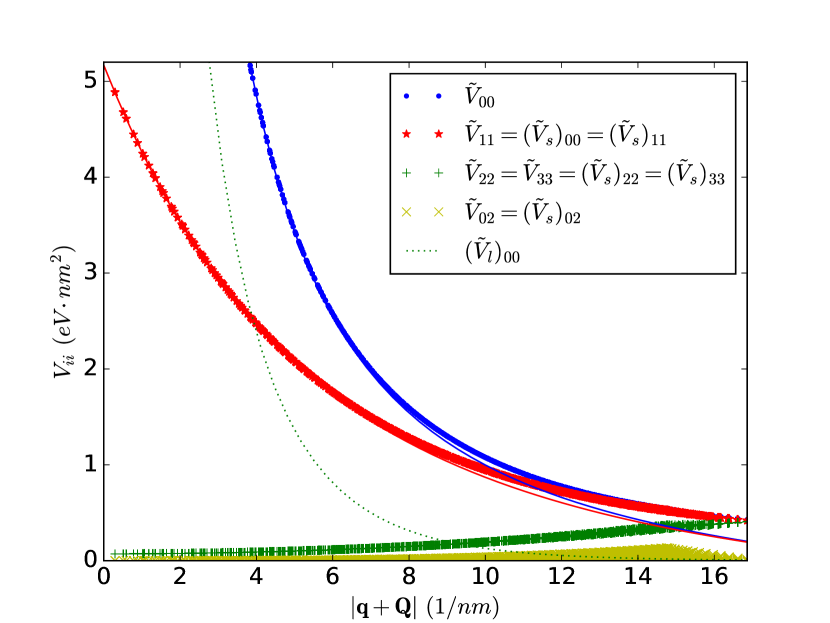
Figure 1: Components of the bare Coulomb interaction in momentum space within the present approximation. The solid lines represent Eqns. 14 and 15, while the dashed line is the long-range part of the interaction, Eqn. 17.

We can also construct a long-wavelength approximation with

$$\tilde{V}_{00}(\mathbf{q},\mathbf{Q},\mathbf{Q})=2\left(\tilde{V}_{0}(|\mathbf{q}+\mathbf{Q}|,0)+\tilde{V}_{0}(|\mathbf{q}+\mathbf{Q}|,d_{il})\right)+u,$$ (14)

where the fitted constant $u=-0.8755\>eV\cdot nm^{2}$ models the short range deviations from the Coulomb law. A corresponding approximation for the interaction between interlayer “dipoles” is given by

$$\tilde{V}_{11}(\mathbf{q},\mathbf{Q},\mathbf{Q})=2\left(\tilde{V}_{0}(|\mathbf{q}+\mathbf{Q}|,0)-\tilde{V}_{0}(|\mathbf{q}+\mathbf{Q}|,d_{il})\right)+u,$$ (15)

where $u$ is the same constant, as it mainly originates from the intralayer interaction. These approximations work well for $|\mathbf{q}+\mathbf{Q}|\lesssim 6$, as can be seen in Fig. 1. At this level of approximation the interaction $\tilde{V}_{ij}$ is diagonal in the indices $i,j$ and the diagonal elements $\tilde{V}_{22}$ and $\tilde{V}_{33}$ are zero.

For the calculation of the dielectric function and the screened interaction we divide the interaction in long-range and short-range parts as follows. We write the intralayer part in real space as

$$V(\mathbf{b}-\mathbf{a})=V_{0}(\sqrt{r^{2}+d_{il}^{2}})+V_{s}(\mathbf{b}-\mathbf{a}),$$ (16)

which defines the short range part $V_{s}$ and includes all contributions beyond the interlayer form $V_{0}(\sqrt{r^{2}+d_{il}^{2}})$. For large values of $r$, $V_{s}$ decays as $r^{-3}$. As the short range part is purely intralayer, the transformed potential $\tilde{V}_{s}$ has the additional symmetry $\tilde{V}_{s,00}=\tilde{V}_{s,11}$ (see Eq. 13). The long-range part $\tilde{V}_{l}$ is not much affected by the short-range intralayer details, and is well-approximated by the continuum form

$$(\tilde{V}_{l})_{ij}(\mathbf{q},\mathbf{Q}_{1},\mathbf{Q}_{2})=4\tilde{V}_{0}(\mathbf{q}+\mathbf{Q}_{1},d_{il})\delta_{\mathbf{Q}_{1}\mathbf{Q}_{2}}\delta_{i0}\delta_{j0},$$ (17)

which includes the convenient cutoff $\exp(-d_{il}q)$, and only the element $\tilde{V}_{l,00}$ is nonzero. The long- and short-range parts are also plotted in Fig. 1.

II.3 Evaluating the matrix elements of P

The computational cost of calculating the Bloch states and energies of the system for some $\mathbf{k}$-grid with $N_{k}$ points scales as $O(N_{a}^{3}N_{k})$, where $N_{a}$ is the number of orbitals in the unit cell. As the Bloch states are needed multiple times during the calculation of the polarization function, we save them to disk and read them back to memory as needed. Calculating the polarization matrix $P(\Omega,\mathbf{q})$ for fixed $\Omega$ and $\mathbf{q}$ from Eq. 6 then scales as $O(N_{a}^{4}N_{k})$, where $N_{a}$ is the number of orbitals in the unit cell. As the moire unit cells of twisted bilayer graphene close to the first magic angle contain of the order of $10^{4}$ atoms, it is not practically possible to evaluate all matrix elements of $P(\Omega,\mathbf{q})$. However, selected matrix elements can be evaluated much faster. Analogously to the interaction in Eqn. 8, we consider the fourier transform

$$\tilde{P}^{SL}_{s_{1}l_{1},s_{2}l_{2}}(\Omega,\mathbf{q},\mathbf{Q}_{1},\mathbf{Q}_{2})=\frac{4}{N_{a}A}\sum_{\mathbf{a}\in l_{1}s_{1},\mathbf{b}\in l_{2}s_{2}}\exp(-i(\mathbf{q}+\mathbf{Q}_{1})\cdot\mathbf{a})P(\Omega,\mathbf{q};\mathbf{a},\mathbf{b})\exp(i(\mathbf{q}+\mathbf{Q}_{2})\cdot\mathbf{b}),$$ (18)

where $\tilde{P}^{SL}(\Omega,\mathbf{q},\mathbf{Q}_{1},\mathbf{Q}_{2})$ is again a matrix in the combined sublattice and layer indices, and the summation is over orbitals in the specific sublattice and layer within the superlattice unit cell.

We can write $\tilde{P}$ in the basis corresponding to Eqn. 12 by performing the transformation $\tilde{P}(\Omega,\mathbf{q},\mathbf{Q}_{1},\mathbf{Q}_{2})=\frac{1}{4}C^{T}\tilde{P}^{SL}(\Omega,\mathbf{q},\mathbf{Q}_{1},\mathbf{Q}_{2})C$. If we define the notation $C_{i}(\mathbf{a})=C_{s(\mathbf{a})l(\mathbf{a}),i}$, where $i$ is again the charge distribution index defined in Eqn. 11 and $s(\mathbf{a})$ and $l(\mathbf{a})$ are the sublattice and layer of the atom at $\mathbf{a}$, we can also write

$$\tilde{P}_{i,j}(\Omega,\mathbf{q},\mathbf{Q}_{1},\mathbf{Q}_{2})=\frac{1}{N_{a}A}\sum_{\mathbf{a},\mathbf{b}}C_{i}(\mathbf{a})\exp(-i(\mathbf{q}+\mathbf{Q}_{1})\cdot\mathbf{a})P(\Omega,\mathbf{q};\mathbf{a},\mathbf{b})\exp(i(\mathbf{q}+\mathbf{Q}_{2})\cdot\mathbf{b})C_{j}(\mathbf{b}),$$ (19)

where the summation goes over all orbitals in the unit cell. This Fourier transform is unitary in the sense that one can think of the factors $C_{i}(\mathbf{b})\exp(i(\mathbf{q}+\mathbf{Q}_{2})\cdot\mathbf{b})/\sqrt{N_{a}}$ as columns in a unitary transformation matrix applied to the matrix $P(\Omega,\mathbf{q})$. Like the interaction $\tilde{V}$, the polarization matrix $\tilde{P}(\Omega,\mathbf{q},\mathbf{Q},\mathbf{Q})$ is approximately diagonal especially at low momenta, as discussed in Section III.1.

The equation for the Fourier transformed polarization function can be written compactly using the overlap

$$M_{n,n^{\prime},i}(\mathbf{q},\mathbf{Q},\mathbf{k})=\frac{1}{\sqrt{N_{a}}}\sum_{\mathbf{b}}C_{i}(\mathbf{b})\exp(i(\mathbf{q}+\mathbf{Q})\cdot\mathbf{b})c_{\mathbf{k},n}(\mathbf{b})^{*}c_{\mathbf{k}-\mathbf{q},n^{\prime}}(\mathbf{b})=\frac{1}{\sqrt{N_{a}}}\sum_{\mathbf{b}}C_{i}(\mathbf{b})\exp(i\mathbf{Q}\cdot\mathbf{b})d_{\mathbf{k},n}(\mathbf{b})^{*}d_{\mathbf{k}-\mathbf{q},n^{\prime}}(\mathbf{b}),$$ (20)

We then have

$$\begin{split}\tilde{P}_{ij}(\Omega,\mathbf{q},\mathbf{Q}_{1},\mathbf{Q}_{2})=\frac{1}{N_{k}A}\sum_{\mathbf{k},n,n^{\prime}}M_{n,n^{\prime},i}(\mathbf{q},\mathbf{Q}_{1},\mathbf{k})^{*}M_{n,n^{\prime},j}(\mathbf{q},\mathbf{Q}_{2},\mathbf{k})\left(\frac{1}{\Omega+\epsilon_{\mathbf{k},n}-\epsilon_{\mathbf{k}^{\prime},n^{\prime}}}-\frac{1}{\Omega-\epsilon_{\mathbf{k},n}+\epsilon_{\mathbf{k}^{\prime},n^{\prime}}}\right)\cdot\\ \cdot\delta(\epsilon_{\mathbf{k},n}<0\land\epsilon_{\mathbf{k}^{\prime},n^{\prime}}>0).\end{split}$$ (21)

Naively evaluating the $M$-factors for fixed $\mathbf{q}$ scales as $O(N_{Q}N_{a}^{3}N_{k})$, where $N_{Q}$ is the number of superlattice momenta. The computation can also be performed as an optimized matrix product by considering the matrices $D^{l}(i,\mathbf{q},\mathbf{Q},\mathbf{k})_{n,\mathbf{b}}=C_{i}(\mathbf{b})\exp(i\mathbf{Q}\cdot\mathbf{b})d_{\mathbf{k},n}(\mathbf{b})^{*}$ and $D^{r}(i,\mathbf{q},\mathbf{Q},\mathbf{k})_{\mathbf{b},n}=d_{\mathbf{k}-\mathbf{q},n}(\mathbf{b})$, so that $M_{i}(\mathbf{q},\mathbf{Q},\mathbf{k})=D^{l}(i,\mathbf{q},\mathbf{Q},\mathbf{k})D^{r}(i,\mathbf{q},\mathbf{Q},\mathbf{k})/\sqrt{N_{a}}$, which is considered as a matrix equation in the $n$ and $\mathbf{b}$ indices.

We can calculate a momentum-space submatrix of $\tilde{P}$ by selecting only some momenta $\mathbf{Q}$. For example, if we only want the momentum-diagonal element, then $N_{Q}=1$. Once the $M$-factors are known, computing $\tilde{P}(\Omega,\mathbf{q})$ from Eq. 21 scales as $O(N_{Q}^{2}N_{a}^{2}N_{k})$, and is subdominant for large enough $N_{a}$, if $N_{Q}$ is kept constant. If we take the full momentum basis, then $N_{Q}=N_{a}/4$ and we regain the $O(N_{a}^{4}N_{k})$ scaling.

II.4 Perturbation theory at $q\rightarrow 0$

For a dieletric where the Fermi energy lies in a gap, the relevant component of the polarization function goes to zero quadratically as $q\rightarrow 0$. This long wavelength component $P_{l}$ can be defined as $P_{l}(\Omega,\mathbf{q})=\tilde{P}_{00}(\Omega,\mathbf{q},\mathbf{0},\mathbf{0})$. We then only need a simplified M-factor that is given by

$$M_{n,n^{\prime}}(\mathbf{q},\mathbf{k})=M_{n,n^{\prime},0}(\mathbf{q},\mathbf{Q}=0,\mathbf{k})=\frac{1}{\sqrt{N_{a}}}\braket{d_{\mathbf{k},n}}{d_{\mathbf{k}^{\prime},n^{\prime}}}.$$ (22)

From the orthogonality of the eigenstates we find that $M_{n,n^{\prime}}(\mathbf{q}=0,\mathbf{k})=\frac{\delta_{n,n^{\prime}}}{\sqrt{N_{a}}}$. The next order term is given by perturbation theory as

$$M_{n,n^{\prime}}(\mathbf{q},\mathbf{k})=\frac{\delta_{n,n^{\prime}}}{\sqrt{N_{a}}}+\frac{1}{\sqrt{N_{a}}}\frac{\braket{d_{\mathbf{k},n}}{-\frac{\partial T^{\prime}_{\mathbf{k}}}{\partial\mathbf{k}}}{d_{\mathbf{k},n^{\prime}}}}{\epsilon_{\mathbf{k},n^{\prime}}-\epsilon_{\mathbf{k},n}}\cdot\mathbf{q}+O(q^{2})$$ (23)

It should be noted that this equation does not hold for degenerate bands $n$ and $n^{\prime}$. However, the degenerate case is never actually needed when the Fermi level is in a gap, or when we calculate the constrained polarization and the Fermi level is within the strongly correlated subspace.

Using the overlap $M$ the long range polarization function can be written as

$$\begin{split}P_{l}(\Omega,\mathbf{q})=\frac{1}{N_{k}A}\sum_{\mathbf{k},n,n^{\prime}}M_{n,n^{\prime}}(\mathbf{q},\mathbf{k})^{*}M_{n,n^{\prime}}(\mathbf{q},\mathbf{k})\cdot\\ \cdot\left(\frac{1}{\Omega+\epsilon_{\mathbf{k},n}-\epsilon_{\mathbf{k}^{\prime},n^{\prime}}}-\frac{1}{\Omega-\epsilon_{\mathbf{k},n}+\epsilon_{\mathbf{k}^{\prime},n^{\prime}}}\right)\cdot\\ \cdot\delta(\epsilon_{\mathbf{k},n}<0\land\epsilon_{\mathbf{k}^{\prime},n^{\prime}}>0).\end{split}$$ (24)

From Eq. 23 it then follows that $P_{l}(\Omega,\mathbf{q}=0)=0$, and

$$\left.\frac{\partial P_{l}(\Omega,\mathbf{q})}{\partial q_{i}}\right|_{\mathbf{q}=0}=0.$$ (25)

Taking the Jacobian, we get

$$\begin{split}\left.\frac{\partial^{2}P_{l}(\Omega,\mathbf{q})}{\partial q_{i}\partial q_{j}}\right|_{\mathbf{q}=0}=\frac{1}{N_{k}N_{a}A}\sum_{\mathbf{k},n,n^{\prime}}\left(\frac{\braket{d_{\mathbf{k},n^{\prime}}}{\frac{\partial T^{\prime}_{\mathbf{k}}}{\partial k_{i}}}{d_{\mathbf{k},n}}}{\epsilon_{\mathbf{k},n^{\prime}}-\epsilon_{\mathbf{k},n}}\frac{\braket{d_{\mathbf{k},n}}{\frac{\partial T^{\prime}_{\mathbf{k}}}{\partial k_{j}}}{d_{\mathbf{k},n^{\prime}}}}{\epsilon_{\mathbf{k},n^{\prime}}-\epsilon_{\mathbf{k},n}}+c.c.\right)\\ \cdot\left(\frac{1}{\Omega+\epsilon_{\mathbf{k},n}-\epsilon_{\mathbf{k},n^{\prime}}}-\frac{1}{\Omega-\epsilon_{\mathbf{k},n}+\epsilon_{\mathbf{k},n^{\prime}}}\right)\delta(\epsilon_{\mathbf{k},n}<0\land\epsilon_{\mathbf{k},n^{\prime}}>0).\end{split}$$ (26)

For the static case $\Omega=0$ this simplifies to

$$\left.\frac{\partial^{2}P_{l}(\Omega=0,\mathbf{q})}{\partial q_{i}\partial q_{j}}\right|_{\mathbf{q}=0}=\frac{-2}{N_{k}N_{a}A}\sum_{\mathbf{k},n,n^{\prime}}\left(\frac{\braket{d_{\mathbf{k},n^{\prime}}}{\frac{\partial T^{\prime}_{\mathbf{k}}}{\partial k_{i}}}{d_{\mathbf{k},n}}\braket{d_{\mathbf{k},n}}{\frac{\partial T^{\prime}_{\mathbf{k}}}{\partial k_{j}}}{d_{\mathbf{k},n^{\prime}}}+c.c.}{(\epsilon_{\mathbf{k},n^{\prime}}-\epsilon_{\mathbf{k},n})^{3}}\right)\delta(\epsilon_{\mathbf{k},n}<0\land\epsilon_{\mathbf{k},n^{\prime}}>0).$$ (27)

One can estimate the region where the quadratic approximation holds by estimating the characteristic scale of the current operator as $\frac{\partial T^{\prime}_{\mathbf{k}}}{\partial k_{i}}\sim v_{F}$, where $v_{F}$ is the Fermi velocity of a single graphene layer, $v_{F}\approx 0.52eVnm$ for our model. The perturbation theory is then expected to be valid as long as $v_{F}q\ll\Delta$. For the full RPA $\Delta$ would be the gap between the subspaces above and below the Fermi level, but for the cRPA it is the gap from the highest state below the Fermi level to the lowest state above the Fermi level that is not within the chosen correlated subspace. Close to the first magic angle the cRPA gap is of the order of $10meV$, which gives a momentum scale of $0.02/nm$. Thus the polarization function should cross over to the dielectric behavior at a relatively large length scale of the order of $50\>nm$. However, the actual gap at $\theta\approx 1.1\>\deg$ is experimentally seen to be closer to $50\>meV$, which is consistent with renormalization of the single layer Fermi velocity by interactions [12], and thus the 2D dielectric behavior might extend to much shorter length scales of $~{}10\>nm$.

III Results

III.1 Polarization function

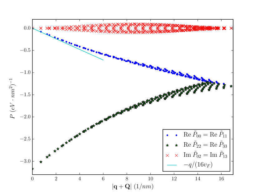
Figure 2: Polarization function of uncoupled graphene layers as a function of the momentum magnitude. The spreading of the points at a given momentum is because the polarization function is not exactly isotropic, especially at larger momenta.

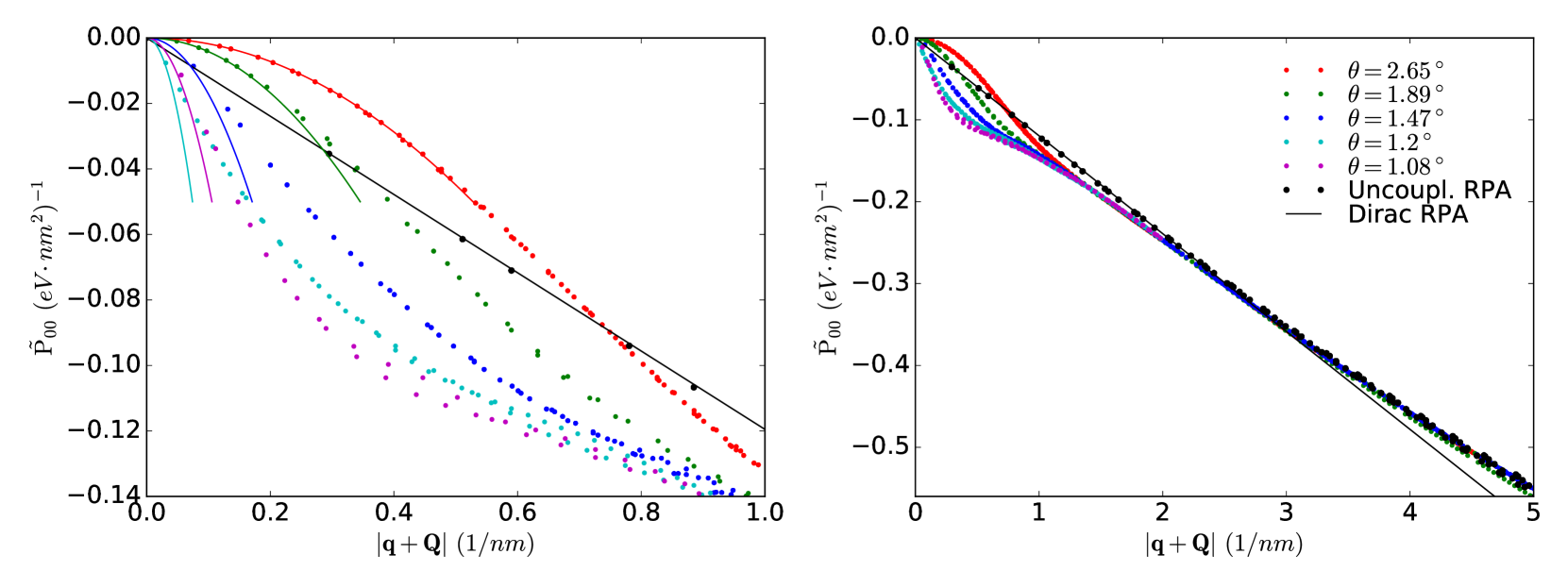
Figure 3: Component $\tilde{P}_{00}$ of the polarization function for different twist angles. Uncoupled RPA refers to the full RPA result for untwisted, uncoupled layers, while Dirac RPA is the analytical result for the Dirac approximation of graphene. The solid curves in the left panel represent the long-wavelength quadratic approximation $\tilde{P}_{00}=-Cq^{2}$, where $C$ is given in table 2. The right panel shows how the polarization approaches the case of uncoupled layers for large momenta.

In this section we present the results for the cRPA polarization function for the TBG $\pi$-band electrons in the static case, i.e. $\Omega=0$. The discussion of the dielectric function and the screening from the $\sigma$-bands and the environment is left to the next section. To better understand the effect of the interlayer coupling, we first briefly discuss the full RPA result for uncoupled, untwisted layers which is plotted in Fig. 2. In this case the polarization is fully momentum diagonal, and has the same form as the short-range part of the interaction,

$$\tilde{P}=\begin{bmatrix}\tilde{P}_{00}&0&\tilde{P}_{02}&0\\ 0&\tilde{P}_{00}&0&\tilde{P}_{02}\\ \tilde{P}_{02}^{*}&0&\tilde{P}_{22}&0\\ 0&\tilde{P}_{02}^{*}&0&\tilde{P}_{22}\\ \end{bmatrix},$$ (28)

where the off-diagonal elements are purely imaginary, and diagonal elements are real so that the whole matrix is hermitian. For small momenta the polarization function $\tilde{P}_{ij}$ is nearly diagonal in the indices $i,j$, and has two branches. The branch $\tilde{P}_{00}=\tilde{P}_{11}$ approaches zero linearly as $\tilde{P}_{00}(q)=-q/(16v_{F})$, which can be derived using the Dirac Hamiltonian approximation of graphene [49]. This branch is associated with charge distributions that are equally distributed between the graphene sublattices. The branch $\tilde{P}_{22}=\tilde{P}_{33}$ is then associated with oppositely charged sublattices, and approaches a constant value for $q\rightarrow 0$. For large enough momenta the polarization starts to deviate from the Dirac approximation and also gains some off-diagonal elements.

We now consider the full tight-binding model of TBG. As for the interaction, we consider an approximation where $\tilde{P}_{i,j}(\Omega,\mathbf{q},\mathbf{Q}_{1},\mathbf{Q}_{2})$ is diagonal in the moire reciprocal lattice momenta $\mathbf{Q}_{1}$ and $\mathbf{Q}_{2}$. We first diagonalize the Bloch Hamiltonian on a momentum grid storing the Bloch states on hard disk, and then evaluate Eq. 21 using the cached results. The grid sizes used were $20\times 20$ moire unit cells for $n=12$ and $n=17$ and $n=27$ and $10\times 10$ for $n=22$ and $n=30$.

Let us first discuss the long-wavelength behavior of the polarization, starting with the component $\tilde{P}_{00}$, which is plotted in Fig. 3. This is the most relevant component of the polarization at long wavelengths, as it couples to the divergent $1/q$-part of the potential. For small enough momentum exchange the polarization becomes quadratic in $q$, $P_{00}(\mathbf{q})=-Cq^{2}$, as discussed in Section II.4. The results for $C$ are presented in table 2. For the smaller unit cells ($n=12$ and $n=17$) we have evaluated the coefficient using numerical integration of Eq. 26 over $\mathbf{k}$. As the numerical integration procedure requires thousands of integrand evaluations, we cannot perform this procedure for the larger unit cells, and instead evaluate Eq. 26 on the same momentum grid as the full polarization function, yielding less accurate estimates. The coefficient $C$ can be converted to the $2D$ polarizability $\alpha_{2D}$ by multiplying with the constant $8k_{c}e^{2}$, where $k_{c}=(4\pi\epsilon_{0})^{-1}$ is the Coulomb constant and the factor of $8$ takes into account layer, sublattice and spin degeneracies. The polarizability $\alpha_{2D}$ determines the crossover scale $r_{0}=2\pi\alpha_{2D}$ such that the interaction is unscreened for $r\gg r_{0}$ [48].

$\theta$ ($\deg$)	$C$ ($1/eV$)	$\alpha_{2D}$ $(nm)$	$r_{0}$ $(nm)$
$2.65$	$0.1796\pm 0.0002$	$2.1$	$13$
$1.89$	$0.419\pm 0.002$	$4.8$	$30$
$1.47$	$1.7$	$20$	$124$
$1.20$	$9.1$	$105$	$659$
$1.08$	$4.5$	$52$	$325$

Table 2: The coefficient $C$ of the quadratic part of the polarization $P_{00}$ and the corresponding 2D polarization length. The length $r_{0}$ determines a scale such that the interaction in freestanding TBG is unscreened for $r\gg r_{0}$. The long-range screening is strongest at the magic angle $\theta=1.20\deg$, and decreases when the angle is either increased or decreased.

Figure 4: Components $\tilde{P}_{11}$, $\tilde{P}_{22}$ and $\tilde{P}_{33}$ of the polarization function for different twist angles. Uncoupled RPA refers to the full RPA result for untwisted, uncoupled layers, while Dirac RPA is the analytical result for the Dirac approximation of graphene.

In contrast to the component $\tilde{P}_{00}$, the other components do not have a fixed value at $q\rightarrow 0$. For the components $\tilde{P}_{22}$ and $\tilde{P}_{33}$ the deviation from the RPA result of uncoupled layers is not very important, as the shift of $\tilde{P}_{22}(q=0)$ and $\tilde{P}_{33}(q=0)$ is small relative to the large absolute value of these components. For $\tilde{P}_{11}$ the effect of the interlayer coupling is more significant, as it lifts the degeneracy between the components $\tilde{P}_{00}$ and $\tilde{P}_{11}$ and makes $\tilde{P}_{11}(q=0)$ non-zero.

For large enough momenta all diagonal components of the polarization function become independent of the twist angle, and approach the polarization of uncoupled layers. This can be understood in a real space perspective: As the coupling between layers is weak relative to the intralayer couplings, the Green’s function for short distances is governed by the intralayer Hamiltonian, and only over longer distances the interlayer scattering processes have sufficient time to affect the propagation. The characteristic time scale of interlayer processes is proportional to $1/V_{il}$, where $V_{il}=0.48eV$ is the hopping amplitude between atoms in the upper and lower layer directly on top of each other, while the characteristic speed of propagation is the Fermi velocity $v_{F}\approx 0.52\>eV\cdot nm$. This gives a length scale of $v_{F}/V_{il}\approx 1\>nm$. For momenta larger than a few times $1/nm$ the polarization is thus expected to be perturbative in $V_{il}$ and not depend on the twist angle, as the average local environment for all twist angles is similar.

In the intermediate momentum regime, where neither the quadratic approximation nor the approximation of uncoupled layers holds, the polarization depends strongly on the twist angle. Close to the magic angle, $|\tilde{P}_{00}|$ is found to be significantly larger than for uncoupled layers. It is interesting to note that the existence of this intermediate region is related to the two independent energy scales: The hopping parameter $V_{il}$ governing the local effect of the interlayer coupling, and the cRPA gap $\Delta$ governing the low-energy, small-$q$ details. In contrast, in most scenarios of gapped graphene the gap $\Delta$ has essentially the same magnitude as the local perturbation, and the crossing from the quadratic behavior to the short range regime happens directly at the momentum scale $\Delta/v_{F}$ with a simpler structure [57, 58].

We have been unable to find a simple model with a few parameters that would satisfactorily fit the polarization function for different angles at all momenta. The model proposed in [55] (Eqn. (4)) for the magic angle case reproduces the large polarization in the intermediate region and the asymptotic Dirac behaviour at large momenta, although we find that the quantitative fit for our magic angle data is not as good as in the case of reference [55]. If it also becomes necessary to model the small-momentum quadratic behaviour, which is not important for the on-site interaction at the magic angle discussed in [55], then a more complicated model with the two crossover scales discussed above is needed. This is important to consider, as the width of the low-energy subspace at $\theta\approx 1.1\>\deg$ is experimentally found to be wider than in theoretical magic-angle models [12, 13, 14], and thus the gap $\Delta$ is also larger, and the quadratic behaviour extends to larger momenta.

III.2 Dielectric function and the long-range interaction

Within the cRPA the screened interaction is calculated from Eq. 7 with the interaction and polarization function discussed in the previous sections. Taking into account background screening from other sources, such as the graphene $\sigma$-bands [50], the total dielectric function can be expressed as

$$\epsilon(\mathbf{q})=\epsilon_{bg}(\mathbf{q})-V(\mathbf{q})P(\mathbf{q}),$$ (29)

where $V$ and $P$ are taken to be $4\times 4$ matrices. We will first discuss the long-range part of the interaction. For the long-range part we assume that the polarization and interaction are diagonal, so that the dielectric function relevant to the long-range interaction is simply $\epsilon(\mathbf{q})=\epsilon_{bg}(\mathbf{q})-V_{00}(\mathbf{q})P_{00}(\mathbf{q})$. We then use Eq. 14 to approximate the interaction $V_{00}$ and a smoothed spline fitted to the polarization data in Fig. 3 to represent the polarization $P_{00}$. The resulting dielectric function with $\epsilon_{bg}=1$, is shown in Fig. 5.

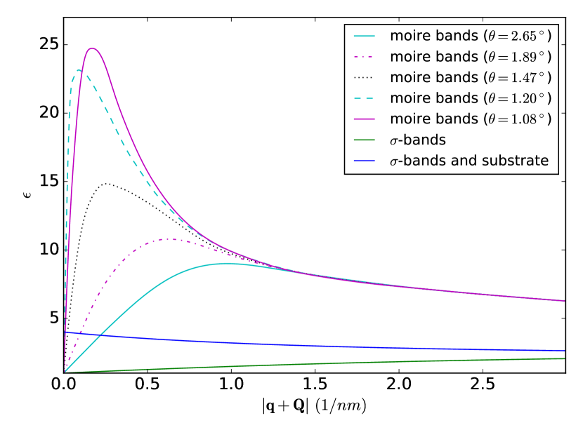
Figure 5: Comparison of the long-range component $\epsilon_{00}$ of the moire band dielectric function without background screening and the background dielectric function $e_{bg}$ with and without the substrate contribution.

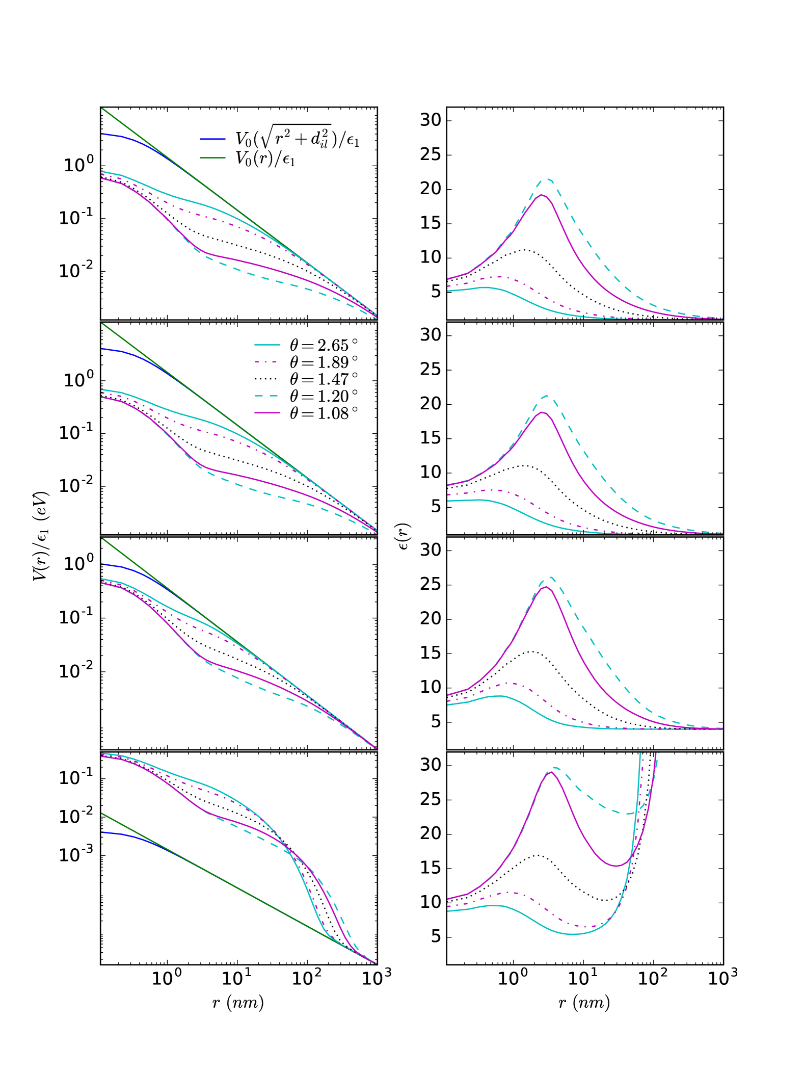
Figure 6: The left panels show the screened long-range part of the coulomb interaction for different twist angles compared to the unscreened interaction, while the right panels show the real-space dielectric function defined as $\epsilon(r)=V_{0}(\sqrt{r^{2}+d^{2}})/W(r)$, where $W(r)$ is the screened interaction. The top row includes screening only from the moire bands, the second highest row from moire bands and graphene $\sigma$-bands, and the second lowest row also from the boron nitride substrate. The lowest row shows how a metallic screening from an electrode $30\>nm$ away from the TBG cuts off the interaction in real space.

To model the screening sources other than the moire bands we use a model where a classical dielectric layer of thickness $D$ and dielectric constant $\epsilon_{2}$ is embedded in a dielectric environment with dielectric constant $\epsilon_{1}$. Following [59] we evaluate the potential in the middle of the layer and calculate the effective dielectric function to be

$$\epsilon_{bg}(q)=\epsilon_{2}\frac{\epsilon_{1}\cosh(qD/2)+\epsilon_{2}\sinh(qD/2)}{\epsilon_{2}\cosh(qD/2)+\epsilon_{1}\sinh(qD/2)},$$ (30)

A special case of this model with $\epsilon_{1}=1$ was used in [50] as an approximation to screening from the $\sigma$-bands of single layer graphene, which we expect to be the main additional source of screening also in free-standing TBG. For the single layer case the parameters are $\epsilon_{2}=2.4$ and $D=D_{graphene}=0.28\>nm$. Expanding Eq. 30 in powers of $q$ gives

$$\epsilon_{bg}(q)=\epsilon_{1}+Dq\frac{\epsilon_{2}^{2}-\epsilon_{1}^{2}}{2\epsilon_{2}}+O(q^{2})=\epsilon_{1}+2\pi\alpha_{2D,\sigma}q+O(q^{2}).$$ (31)

The effective 2D screening constant for the single layer case is then $\alpha^{graphene}_{2D,\sigma}\approx 0.044\>nm$. For TBG this value is expected to double to $\alpha^{TBG}_{2D,\sigma}\approx 0.088\>nm$, as the $\sigma$-band screening now comes from both layers. Comparing this value to table 2, we see that the $\sigma$-bands are insignificant for the long-range screening in comparison to the moire bands.

To fully treat the local and intermediate-range effects of the $\sigma$-bonding orbitals would require DFT calculations for the bilayer system, which is beyond the scope of this work. However, it is reasonable to assume that the short range screening constant is roughly the same as for the single layer case. To estimate the overall importance of the $\sigma$-bands we then use Eq. 30 and set $D=D_{TBG}=0.56\>nm$, i.e. twice the value found in [50], which correctly produces the long-distance and short-distance limits discussed above. The true $\epsilon_{\sigma}$ is expected to have a more complicated structure, but the relevant length scales $D_{graphene}$, $D_{TBG}$ and the interlayer distance $d_{il}\approx 0.334\>nm$ are of similar magnitude, so that the crossover to the large-momentum behaviour is expected to happen at a scale of $2...4\>/nm$. The estimated contribution of the $\sigma$-bands to the dielectric function is plotted in Fig. 5.

In real experiments the TBG is not free-standing, but typically sandwiched between boron nitride layers with thickness of $10\>nm$ to $30\>nm$ [2]. This can be at least qualitatively modeled by setting $\epsilon_{1}\approx 4$ [60], leading to a background screening with a negative $\alpha_{2D}$. This background screening model is also shown in Fig. 5. On top of the boron nitride layers the experimental devices also contain metallic gate electrodes, which are used e.g. to tune the fermi level in the system. This will provide metallic screening [55], which cuts off the interaction at the momentum scale $1/D_{gate}$, where $D_{gate}\approx 10\>nm...30\>nm$ is the distance of the electrode from the TBG. The corresponding background dielectric function (not shown) can be modeled qualitatively by neglecting the $\sigma$-band screening and setting $D=2D_{gate}\approx 60\>nm$, $\epsilon_{1}=1000$ and $\epsilon_{2}=4.0$, similarly to the model in [55]. In the following we will calculate the interaction in real space, and show the effect of the different background dielectric functions.

We numerically calculate the Fourier transform of the screened long-range part of the interaction defined in equation 17. This leads to the integral

$$W(r)=\int\frac{d^{2}\mathbf{q}}{(2\pi)^{2}}\exp(i\mathbf{r}\cdot\mathbf{q})\tilde{V}_{0}(\mathbf{q},d_{il})/\epsilon_{00}(\mathbf{q}),$$ (32)

where $\tilde{V}_{0}$ is defined in equation 10. Here the factor $\exp(-qd_{il})$ included in $\tilde{V}_{0}$ provides a convenient cutoff with the scale $1/d_{il}\approx 3/nm$. We plot the screened real-space interaction in the left column of Fig. 6, and the real-space dielectric function defined as $\epsilon(r)=V_{0}(\sqrt{r^{2}+d^{2}})/W(r)$ in the right column. In the long-range limit the moire bands do not provide any screening, so that $\epsilon(r\rightarrow\infty)=\epsilon_{bg}(q=0)=\epsilon_{1}$. The peak in the momentum-space dielectric function (Fig. 5), which close to the magic angle is found at $q\sim 0.25/nm$, translates into a real space peak at $r\sim 4\>nm$. Comparing the two upper rows in Fig. 6, the $\sigma$-band screening is found to be rather insignificant. When the boron nitride substrate is taken into account (third row of Fig. 6), the peak value of the dielectric function at the magic angle reaches $\epsilon\sim 25$. In this model the boron nitride layers are infinitely thick, so that the screening continues to long distances. Finally, the lowest panels demonstrate how the interaction is cut off by screening from metallic electrodes $30\>nm$ away from the TBG.

The Coulomb interaction screened by a classical two-dimensional dielectric layer with polarizability $\alpha_{2D}$ can also be calculated analytically, yielding [48]

$$W_{2D}(r)=k_{c}\frac{e^{2}}{4\alpha_{2D}}\left(H_{0}(r/r_{0})-Y_{0}(r/r_{0})\right),$$ (33)

where the $r_{0}=2\pi\alpha_{2D}$, $k_{c}$ is the Coulomb constant, $H_{0}$ is a Struve function and $Y_{0}$ is a Bessel function of the second kind. This is a good approximation to the screened interaction of freestanding TBG beyond a length scale that is essentially determined by the cRPA gap as discussed in section II.4. We plot a comparison of this approximation and the full screened Coulomb interaction in Fig. 7. The screening effect is well-approximated beyond a few tens of nanometers at the magic angle, and the approximation improves when moving away from the magic angle.

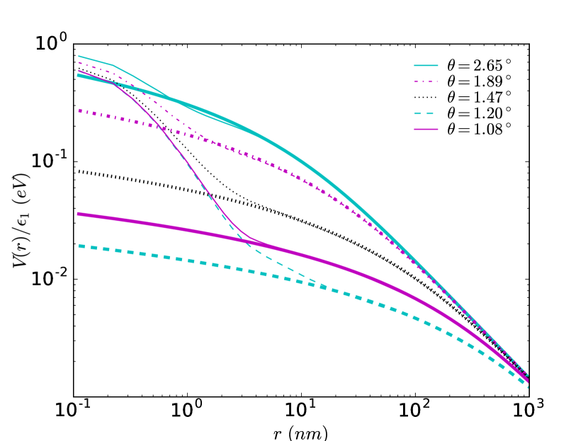
Figure 7: Comparison of the long-range component of the screened Coulomb interaction (thin lines) to the 2D dielectric screening form, Eq. 33 (thick lines). Here we have used the interaction without the screening from the $\sigma$-bands and the environment.

III.3 Interactions in the hexagonal lattice models

The real-space dielectric function is useful in connection with the “fractional point charge approximation” introduced in [33]. Within this approximation, each Wannier orbital consists of three point charges of strength $e/3$ positioned in the middle of three neighbouring AA-regions of the moire lattice. In this section we will estimate the screened direct Coulomb potential between these $e/3$ charges based on the screened interaction taking into account the screening from the substrate (i.e. the second lowest panel in Fig. 6).

To estimate the “on-site term” $U$ for the $e/3$ charges we calculate the potential between two identical gaussian charge distributions with different variances $\sigma$ and plot the result in Fig. 8. We also calculate an effective dielectric constant $\epsilon_{U}$ for the on-site contribution as the ratio of the screened and unscreened potentials. This yields values in the range $18$ to $22$ for a wide range of $\sigma$. Using numerical data for the Wannier functions and assuming a constant dielectric function $\epsilon$, the on-site interaction $U$ was evaluated in [33] to be $U\approx(e/3)^{2}/(0.28\epsilon L_{m})$. Here we take the value of the dielectric function $\epsilon_{U}$ from Fig. 8 at $\sigma=0.28L_{m}$, and then plug in the moire lattice constant $L_{m}$ and the effective dielectric constant $\epsilon=4\pi\epsilon_{0}\epsilon_{U}$ to the above expression for $U$. Directly reading off $U$ from the upper panel of Fig. 8 at $\sigma=0.28L_{m}$ yields similar results. For the rest of the potentials we use the point charge approximation [33] and directly use the value of the real-space dielectric function for the distance between the point charges. The results for the magic angle are plotted in Fig. 9. It is interesting to observe that the screened interaction decays slower than $1/r$ for intermediate length scales, as demonstrated in the inset, which is a feature of the 2D screened interaction, Eqn. 33.

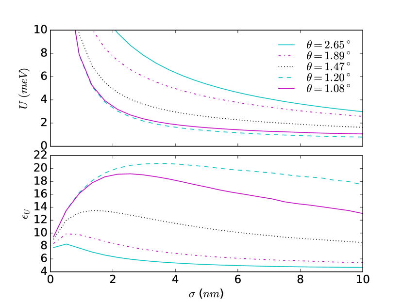
Figure 8: Upper panel: The screened potential between two gaussian charge distributions of total charge $e/3$ and width $\sigma$. This approximates the on-site contribution of the $e/3$ fractional charge approximation [33]. Lower panel: The ratio of the screened potential and the bare potential, giving the effective dielectric constant of the on-site contribution for the fractional charges.

We end this section by tabulating the Coulomb interaction terms for the full Wannier orbitals in the magic angle case up to the fourth nearest neighbour in Table 3, which can easily be evaluated using Fig. 9. We have also similarly evaluated the interaction parameters for two other twist angles with the corresponding values of $L_{m}$ and $\epsilon_{U}$. For the magic angle case the short-range interaction terms are about $10\>meV$, which is roughly the same as the total bandwidth of the four low-energy bands, and the Coulomb effects are thus expected to be important. However, as mentioned in the introduction section, it could be that the actual bandwidth at the angle $\theta\approx 1.1\>\deg$ used in the transport experiments [1, 2, 3, 4, 5] is considerably larger, several tens of $meV$ [12, 13, 14]. Nevertheless, the Coulomb interaction is of the same order of magnitude as the experimentally measured width of the van Hove singularities [12]. Our estimate of the on-site interaction $V_{0}$ of the full Wannier orbitals is a bit smaller than the estimates of the on-site interaction given in [55]. The differences are perhaps partly because our dielectric function attains slightly larger values than that in reference [55], but also because we use the fractional charge picture of the Wannier functions, while reference [55] uses a momentum space integral.

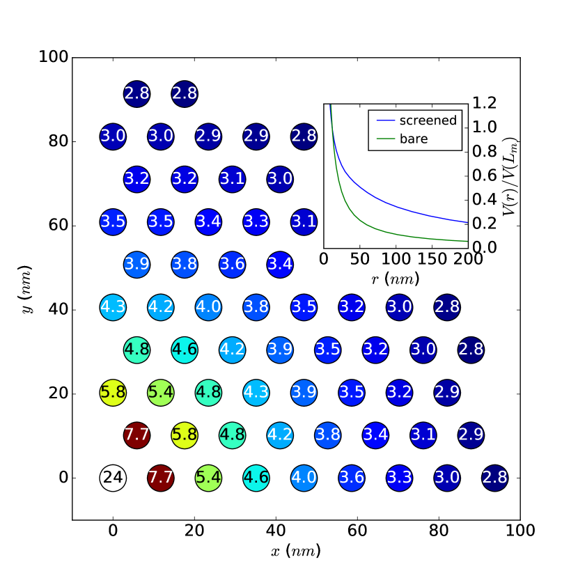
Figure 9: Main panel: The potential between the $e/3$ charges in the AA-regions of the moire lattice in units of $0.1\>meV$. Inset: Comparison of the decay of the bare and the screened interaction.

$\theta$	$\epsilon_{U}$	$U$	$V_{0}$	$V_{1}$	$V_{2}$	$V_{3}$	$V_{4}$
$1.47\deg$	$13$	$4.6$	$25$	$22$	$19$	$18$	$14$
$1.20\deg$	$20$	$2.4$	$12$	$10$	$8.0$	$7.7$	$5.5$
$1.08\deg$	$19$	$2.3$	$13$	$12$	$9.8$	$9.5$	$7.6$

Table 3: Estimated $n$:th nearest neighbour interactions $V_{n}$ (energy unit $meV$) for the full Wannier orbitals for the magic angle case $\theta=1.20$ and for TBG slightly above and below the magic angle. This can be compared with Table I in [33]. U here denotes the “on-site” term of the $e/3$ charges, while $V_{0}$ is the on-site term for the full Wannier orbitals.

III.4 Short range contributions

In the previous section we discussed the screening of the long-range part of the interaction. To complete the treatment we also need to estimate the remaining short-range contribution. To ensure a hermitian interaction matrix we write the screened interaction in the form

$$\begin{split}W(\mathbf{q})&=\epsilon(\mathbf{q})^{-1}V(\mathbf{q})\\ &=\frac{1}{2}\left(\epsilon(\mathbf{q})^{-1}V(\mathbf{q})+V(\mathbf{q})(\epsilon(\mathbf{q})^{\dagger})^{-1}\right).\end{split}$$ (34)

The short range part $W_{s}(\mathbf{q})$ of the interaction is then obtained by replacing $V$ on the second line by the bare short-range interaction. As the short-range interaction is insensitive to the small-$q$ details of the polarization function, we use here simply the RPA dielectric function of uncoupled graphene layers. We do not consider here the screening from the $\sigma$-bands or the substrate. We take the Fourier transform of the bare intralayer interaction numerically, and use the continuum approximation 10 for the bare interlayer interaction.

The screened short-range part of the interaction is plotted in Fig. 10. We note that, although the bare short range interaction defined in Eq. 16 is purely intralayer, the screened interaction has an interlayer component due to the interlayer parts of the dielectric matrix, where the full interaction still enters. The interlayer part of the screened short-range interaction is negative, which compensates for some screening missing from the long-range part, but the total Coulomb interaction is still always positive. The intralayer part is positive and compensates for the “artificial” short-range screening $\exp(-qd_{il})$ introduced to the long-range part.

The short-range part produces non-negligible corrections to intra- and interlayer interactions even beyond $r\sim 10\>nm$. However, the mean of the interlayer and intralayer corrections is quite small already for $r\gtrsim 0.25\>nm$, corresponding to the next-nearest neighbour interaction within the graphene layer. Thus the long-range part of the interaction should be a reasonably good approximation for everything but the on-site and nearest neighbour interactions provided that the charge distribution is equal in both layers. The correction for the intralayer on-site term of the microscopic model is roughly $5\>eV$. Within the fractional charge picture the $e/3$ charge is distributed to one AA-region of the unit cell. Estimating that this region contains of the order of $1000$ atoms and the charge is equally distributed over each atom, the on-site terms contribute an energy of $0.5\>meV$. Thus the contribution from the short-range part to the on-site term of the $e/3$ charges is likely to be less than $1\>meV$. Using similar arguments it was concluded in [61] that the microscopic on-site contribution is relatively unimportant. Taking into account the distance dependent screening from the moire bands increases the importance of the short range contributions because of the stronger screening at intermediate distances compared to very short ones. This can be taken into account by slightly reducing $\epsilon_{U}$ (see table 3).

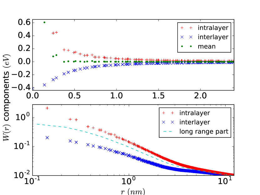
Figure 10: Upper panel: Intralayer and interlayer components of the short-range part of the screened interaction as a function of the planar distance. The mean of the two components is also shown. Lower panel: The full intralayer and interlayer interaction for $\theta=1.2$ calculated as the sum of the long-range part and the short-range components. Here only the screening from the moire bands has been taken into account.

IV Discussion and Conclusions

An accurate low-energy theory of twisted bilayer graphene based on microscopic tight-binding models seems to be a realistic goal, although a more complete understanding of e.g. lattice relaxation effects is still needed. The simplest models have been built on the four lowest moire bands [33, 34, 35]. Here we have discussed screening of the Coulomb interaction by the moire bands outside this model space. As expected for a two-dimensional gapped system, the cRPA polarization function is quadratic for small momentum exchange with a 2D polarizability $\alpha_{2D}$ depending on the twist angle. The polarizability attains a peak value of $\alpha_{2D}\approx 100\>nm$ at the magic angle, and is of the order of tens of nanometers when the angle is tuned $\sim 0.3$ degrees away from the peak. The quadratic approximation is valid up to a momentum scale that is expected to follow $q\sim\Delta/v_{F}$, where $\Delta$ is the distance from the Fermi level to the lowest screening bands. In freestanding TBG the 2D screened Coulomb interaction [48] is then a reasonable approximation for $r\gtrsim v_{F}/\Delta$. At the magic angle with $\Delta\sim 10\>meV$ this is a relatively large distance, $r\sim 50\>nm$. However, as the experimentally observed bandwidth and $\Delta$ e.g. at the angle $\theta\approx 1.1\deg$ seem significantly larger [12, 13, 14], this approximation might be sufficient for length scales somewhat larger than the moire lattice constant.

For large enough momenta the polarization and the dielectric function of freestanding TBG become independent of the twist angle and start to approach that of unhybridized graphene layers. The momentum scale for this transition is expected to depend on the strength $V_{il}$ of the interlayer hopping parameters as $q\sim V_{il}/v_{F}\approx 1\>nm$. In the intermediate region between the low- and high-momentum limits the dielectric function has a maximum which is largest for twist angles close to the magic angle, attaining values of $\epsilon(q_{max})\approx 25$. Screening from the moire bands dominates effects from the graphene $\sigma$-bands, although a more accurate estimation of $\sigma$-band effects at short distances would require density functional theory calculations.

While dealing with the full tight-binding model is computationally costly, it is also flexible and can easily be adapted to changes in the tight-binding parameters, for example. Preliminary results indicate that doping the system by two electrons per moire cell does not change the essential features of the polarization function. An interesting experimental development is increasing the interlayer coupling with pressure [3], which would mean increasing the local interlayer hopping scale $V_{il}$. Increased pressure is thus expected to enlarge the region where the polarization function shows strong dependence on the twist angle.

Screening from the TBG environment includes contributions from the substrate, typically boron nitride, and metallic screening from the gate electrodes. The effect of the boron nitride layers is mainly to renormalize the long-range interaction, while most of the momentum dependence of the dielectric function still arises from the intrinsic TBG screening. In contrast, metallic screening from the electrodes will provide an interaction cutoff distance proportional to their distance from the TBG. This provides interesting possibilities for experiments: As a result of the 2D screening behaviour, the long-range interaction without the metallic screening decays slowly, even slower than $1/r$. A device with a large separation of the electrodes from the TBG is thus expected to have strong extended interactions, while a small separation leads to more local interactions. A comparison of the phase diagrams for such devices might give clues about the mechanism of the superconductivity. For instance, it is theoretically expected that the $d$-wave superconductivity in the square lattice Hubbard model is suppressed by nearest neighbour repulsion [62], although retardation effects could reverse this picture [63].

Our results can be compared to the continuum model calculations of reference [55], where especially the tuning of the short-range interaction by changing the dielectric environment is discussed. There the cRPA screened on-site interaction in the magic-angle case was found to be $40\>meV$ for the freestanding TBG, while a metallic gate $3\>nm$ from the TBG reduces this to $28\>meV$. Thus the gate has to be relatively close to significantly alter the on-site interaction, and at larger gate distances the main effect is on the long-range part. Quantitatively our estimates for the on-site contribution in the freestanding case are a bit smaller than in [55], $12\>meV$ to $25\>meV$ within $\pm 0.3\deg$ of the magic angle. While the calculations in [55] and our work provide a reasonable picture of the screening, improved microscopic models with the magic angles and bandwidths coinciding with the experimentally measured ones are still needed to truly fix the parameters of the low-energy model. It has also been shown that the cRPA can overestimate the screening in some models [64, 65], especially at short distances. Indeed, a more accurate treatment of the short-range interactions free of the momentum-diagonal approximation made in our work would be desirable.

Assuming that the superconductivity and insulating states close to half-filling of the conduction and valence bands result from strong correlation effects, the scale of the interaction should roughly correspond to the width of the van Hove singularities, which has been measured to be of the order of $10\>meV$ [12]. This is indeed the scale of the interactions produced by the cRPA calculation, and thus our results are compatible with a picture where the screened Coulomb interaction is the driving force behind the observed insulating states. As noted e.g. in [55], one thing that speaks against this picture is the very small thermal activation gap of $0.3\>meV$ in the insulating states at half-filling of the valence or conduction bands [2], as compared to the effective interaction strength, although spectroscopy experiments indicate larger gaps by an order of magnitude [12], and it has been suggested that the small transport gaps could be due to disorder averaging [12].

Finally, we consider TBG at the charge neutrality point. A long-standing theoretical problem has been the stability of Dirac liquids under the Coulomb interaction [66, 67, 68, 69], and it would be interesting to study how this problem is modified by the 2D screening and the doubling of the number of components as compared to single-layer graphene. It has been proposed that TBG at charge neutrality is close to a quantum critical point where a Dirac mass term is spontaneously generated [70]. As the extended interaction terms play an important role for such phase transitions in Dirac systems [70, 69], the possibility to tune them experimentally is interesting also in this context.

Note added: After the completion of this work, we became aware of a recent preprint that also considers the cRPA polarization function of twisted bilayer graphene [71].

References

- Cao et al. [2018a] Y. Cao, V. Fatemi, S. Fang, K. Watanabe, T. Taniguchi, E. Kaxiras, and P. Jarillo-Herrero, Unconventional superconductivity in magic-angle graphene superlattices, Nature 556, 43 (2018a).
- Cao et al. [2018b] Y. Cao, V. Fatemi, A. Demir, S. Fang, S. L. Tomarken, J. Y. Luo, J. D. Sanchez-Yamagishi, K. Watanabe, T. Taniguchi, E. Kaxiras, R. C. Ashoori, and P. Jarillo-Herrero, Correlated insulator behaviour at half-filling in magic-angle graphene superlattices, Nature 556, 80 (2018b).
- Yankowitz et al. [2019] M. Yankowitz, S. Chen, H. Polshyn, Y. Zhang, K. Watanabe, T. Taniguchi, D. Graf, A. F. Young, and C. R. Dean, Tuning superconductivity in twisted bilayer graphene, Science 363, 1059 (2019).
- Codecido et al. [2019] E. Codecido, Q. Wang, R. Koester, S. Che, H. Tian, R. Lv, S. Tran, K. Watanabe, T. Taniguchi, F. Zhang, M. Bockrath, and C. N. Lau, Correlated Insulating and Superconducting States in Twisted Bilayer Graphene Below the Magic Angle, arXiv e-prints , arXiv:1902.05151 (2019).
- Sharpe et al. [2019] A. L. Sharpe, E. J. Fox, A. W. Barnard, J. Finney, K. Watanabe, T. Taniguchi, M. A. Kastner, and D. Goldhaber-Gordon, Emergent ferromagnetism near three-quarters filling in twisted bilayer graphene, 365, 605 (2019).
- Lopes dos Santos et al. [2007] J. M. B. Lopes dos Santos, N. M. R. Peres, and A. H. Castro Neto, Graphene bilayer with a twist: Electronic structure, Phys. Rev. Lett. 99, 256802 (2007).
- Suárez Morell et al. [2010] E. Suárez Morell, J. D. Correa, P. Vargas, M. Pacheco, and Z. Barticevic, Flat bands in slightly twisted bilayer graphene: Tight-binding calculations, Phys. Rev. B 82, 121407 (2010).
- Bistritzer and MacDonald [2011] R. Bistritzer and A. H. MacDonald, Moiré bands in twisted double-layer graphene, Proceedings of the National Academy of Sciences of the United States of America 108, 12233 (2011).
- Yoo et al. [2019] H. Yoo, R. Engelke, S. Carr, S. Fang, K. Zhang, P. Cazeaux, S. H. Sung, R. Hovden, A. W. Tsen, T. Taniguchi, K. Watanabe, G.-C. Yi, M. Kim, M. Luskin, E. B. Tadmor, E. Kaxiras, and P. Kim, Atomic and electronic reconstruction at the van der Waals interface in twisted bilayer graphene, Nature Materials 18, 448 (2019).
- Guinea and Walet [2019] F. Guinea and N. R. Walet, Continuum models for twisted bilayer graphene: Effect of lattice deformation and hopping parameters, Phys. Rev. B 99, 205134 (2019).
- Lin and Tománek [2018] X. Lin and D. Tománek, Minimum model for the electronic structure of twisted bilayer graphene and related structures, Phys. Rev. B 98, 081410 (2018).
- Kerelsky et al. [2019] A. Kerelsky, L. J. McGilly, D. M. Kennes, L. Xian, M. Yankowitz, S. Chen, K. Watanabe, T. Taniguchi, J. Hone, C. Dean, A. Rubio, and A. N. Pasupathy, Maximized electron interactions at the magic angle in twisted bilayer graphene, Nature 572, 95 (2019).
- Choi et al. [2019] Y. Choi, J. Kemmer, Y. Peng, A. Thomson, H. Arora, R. Polski, Y. Zhang, H. Ren, J. Alicea, G. Refael, F. von Oppen, K. Watanabe, T. Taniguchi, and S. Nadj-Perge, Imaging Electronic Correlations in Twisted Bilayer Graphene near the Magic Angle, arXiv e-prints , arXiv:1901.02997 (2019).
- Liu et al. [2019] Y.-W. Liu, J.-B. Qiao, C. Yan, Y. Zhang, S.-Y. Li, and L. He, Magnetism near half-filling of a van hove singularity in twisted graphene bilayer, Phys. Rev. B 99, 201408 (2019).
- Classen et al. [2019] L. Classen, C. Honerkamp, and M. M. Scherer, Competing phases of interacting electrons on triangular lattices in moiré heterostructures, Phys. Rev. B 99, 195120 (2019).
- Dodaro et al. [2018] J. F. Dodaro, S. A. Kivelson, Y. Schattner, X. Q. Sun, and C. Wang, Phases of a phenomenological model of twisted bilayer graphene, Phys. Rev. B 98, 075154 (2018).
- Fidrysiak et al. [2018] M. Fidrysiak, M. Zegrodnik, and J. Spałek, Unconventional topological superconductivity and phase diagram for an effective two-orbital model as applied to twisted bilayer graphene, Phys. Rev. B 98, 085436 (2018).
- Guo et al. [2018] H. Guo, X. Zhu, S. Feng, and R. T. Scalettar, Pairing symmetry of interacting fermions on a twisted bilayer graphene superlattice, Phys. Rev. B 97, 235453 (2018).
- Xu and Balents [2018] C. Xu and L. Balents, Topological superconductivity in twisted multilayer graphene, Phys. Rev. Lett. 121, 087001 (2018).
- Kang and Vafek [2019] J. Kang and O. Vafek, Strong coupling phases of partially filled twisted bilayer graphene narrow bands, Phys. Rev. Lett. 122, 246401 (2019).
- Kennes et al. [2018] D. M. Kennes, J. Lischner, and C. Karrasch, Strong correlations and superconductivity in twisted bilayer graphene, Phys. Rev. B 98, 241407 (2018).
- Tang et al. [2019] Q.-K. Tang, L. Yang, D. Wang, F.-C. Zhang, and Q.-H. Wang, Spin-triplet -wave pairing in twisted bilayer graphene near -filling, Phys. Rev. B 99, 094521 (2019).
- Thomson et al. [2018] A. Thomson, S. Chatterjee, S. Sachdev, and M. S. Scheurer, Triangular antiferromagnetism on the honeycomb lattice of twisted bilayer graphene, Phys. Rev. B 98, 075109 (2018).
- Venderbos and Fernandes [2018] J. W. F. Venderbos and R. M. Fernandes, Correlations and electronic order in a two-orbital honeycomb lattice model for twisted bilayer graphene, Phys. Rev. B 98, 245103 (2018).
- Pizarro et al. [2019] J. M. Pizarro, M. J. Calderón, and E. Bascones, The nature of correlations in the insulating states of twisted bilayer graphene, Journal of Physics Communications 3, 035024 (2019).
- Yuan and Fu [2018] N. F. Q. Yuan and L. Fu, Model for the metal-insulator transition in graphene superlattices and beyond, Phys. Rev. B 98, 045103 (2018).
- Roy and Juričić [2019] B. Roy and V. Juričić, Unconventional superconductivity in nearly flat bands in twisted bilayer graphene, Phys. Rev. B 99, 121407 (2019).
- Sherkunov and Betouras [2018] Y. Sherkunov and J. J. Betouras, Electronic phases in twisted bilayer graphene at magic angles as a result of van hove singularities and interactions, Phys. Rev. B 98, 205151 (2018).
- You and Vishwanath [2019] Y.-Z. You and A. Vishwanath, Superconductivity from valley fluctuations and approximate SO(4) symmetry in a weak coupling theory of twisted bilayer graphene, npj Quantum Materials 4, 16 (2019).
- Laksono et al. [2018] E. Laksono, J. N. Leaw, A. Reaves, M. Singh, X. Wang, S. Adam, and X. Gu, Singlet superconductivity enhanced by charge order in nested twisted bilayer graphene fermi surfaces, Solid State Communications 282, 38 (2018).
- Padhi et al. [2018] B. Padhi, C. Setty, and P. W. Phillips, Doped twisted bilayer graphene near magic angles: Proximity to wigner crystallization, not mott insulation, Nano Letters 18, 6175 (2018), pMID: 30185049.
- González and Stauber [2019] J. González and T. Stauber, Kohn-luttinger superconductivity in twisted bilayer graphene, Phys. Rev. Lett. 122, 026801 (2019).
- Koshino et al. [2018] M. Koshino, N. F. Q. Yuan, T. Koretsune, M. Ochi, K. Kuroki, and L. Fu, Maximally localized wannier orbitals and the extended hubbard model for twisted bilayer graphene, Phys. Rev. X 8, 031087 (2018).
- Kang and Vafek [2018] J. Kang and O. Vafek, Symmetry, maximally localized wannier states, and a low-energy model for twisted bilayer graphene narrow bands, Phys. Rev. X 8, 031088 (2018).
- Po et al. [2018] H. C. Po, L. Zou, A. Vishwanath, and T. Senthil, Origin of mott insulating behavior and superconductivity in twisted bilayer graphene, Phys. Rev. X 8, 031089 (2018).
- Seo et al. [2019] K. Seo, V. N. Kotov, and B. Uchoa, Ferromagnetic mott state in twisted graphene bilayers at the magic angle, Phys. Rev. Lett. 122, 246402 (2019).
- Su and Lin [2018] Y. Su and S.-Z. Lin, Pairing symmetry and spontaneous vortex-antivortex lattice in superconducting twisted-bilayer graphene: Bogoliubov-de gennes approach, Phys. Rev. B 98, 195101 (2018).
- Peltonen et al. [2018] T. J. Peltonen, R. Ojajärvi, and T. T. Heikkilä, Mean-field theory for superconductivity in twisted bilayer graphene, Phys. Rev. B 98, 220504 (2018).
- Julku et al. [2019] A. Julku, T. J. Peltonen, L. Liang, T. T. Heikkilä, and P. Törmä, Superfluid weight and Berezinskii-Kosterlitz-Thouless transition temperature of twisted bilayer graphene, arXiv e-prints , arXiv:1906.06313 (2019).
- Hu et al. [2019] X. Hu, T. Hyart, D. I. Pikulin, and E. Rossi, Geometric and conventional contribution to superfluid weight in twisted bilayer graphene, arXiv e-prints , arXiv:1906.07152 (2019).
- Choi and Choi [2018] Y. W. Choi and H. J. Choi, Strong electron-phonon coupling, electron-hole asymmetry, and nonadiabaticity in magic-angle twisted bilayer graphene, Phys. Rev. B 98, 241412 (2018).
- Wu et al. [2018] F. Wu, A. H. MacDonald, and I. Martin, Theory of phonon-mediated superconductivity in twisted bilayer graphene, Phys. Rev. Lett. 121, 257001 (2018).
- Wu [2019] F. Wu, Topological chiral superconductivity with spontaneous vortices and supercurrent in twisted bilayer graphene, Phys. Rev. B 99, 195114 (2019).
- Lian et al. [2019] B. Lian, Z. Wang, and B. A. Bernevig, Twisted bilayer graphene: A phonon-driven superconductor, Phys. Rev. Lett. 122, 257002 (2019).
- Liu et al. [2018] C.-C. Liu, L.-D. Zhang, W.-Q. Chen, and F. Yang, Chiral spin density wave and superconductivity in the magic-angle-twisted bilayer graphene, Phys. Rev. Lett. 121, 217001 (2018).
- Isobe et al. [2018] H. Isobe, N. F. Q. Yuan, and L. Fu, Unconventional superconductivity and density waves in twisted bilayer graphene, Phys. Rev. X 8, 041041 (2018).
- Rademaker and Mellado [2018] L. Rademaker and P. Mellado, Charge-transfer insulation in twisted bilayer graphene, Phys. Rev. B 98, 235158 (2018).
- Cudazzo et al. [2011] P. Cudazzo, I. V. Tokatly, and A. Rubio, Dielectric screening in two-dimensional insulators: Implications for excitonic and impurity states in graphane, Phys. Rev. B 84, 085406 (2011).
- Kotov et al. [2012] V. N. Kotov, B. Uchoa, V. M. Pereira, F. Guinea, and A. H. Castro Neto, Electron-electron interactions in graphene: Current status and perspectives, Rev. Mod. Phys. 84, 1067 (2012).
- Wehling et al. [2011] T. O. Wehling, E. Şaşıoğlu, C. Friedrich, A. I. Lichtenstein, M. I. Katsnelson, and S. Blügel, Strength of effective coulomb interactions in graphene and graphite, Phys. Rev. Lett. 106, 236805 (2011).
- Nam and Koshino [2017] N. N. T. Nam and M. Koshino, Lattice relaxation and energy band modulation in twisted bilayer graphene, Phys. Rev. B 96, 075311 (2017).
- Aryasetiawan et al. [2004] F. Aryasetiawan, M. Imada, A. Georges, G. Kotliar, S. Biermann, and A. I. Lichtenstein, Frequency-dependent local interactions and low-energy effective models from electronic structure calculations, Phys. Rev. B 70, 195104 (2004).
- Vaugier et al. [2012] L. Vaugier, H. Jiang, and S. Biermann, Hubbard and hund exchange in transition metal oxides: Screening versus localization trends from constrained random phase approximation, Phys. Rev. B 86, 165105 (2012).
- Shinaoka et al. [2015] H. Shinaoka, M. Troyer, and P. Werner, Accuracy of downfolding based on the constrained random-phase approximation, Phys. Rev. B 91, 245156 (2015).
- Pizarro et al. [2019] J. M. Pizarro, M. Rösner, R. Thomale, R. Valentí, and T. O. Wehling, Internal screening and dielectric engineering in magic-angle twisted bilayer graphene, arXiv e-prints , arXiv:1904.11765 (2019).
- Note [1] In our notation the polarization function corresponds to that of a single Dirac cone, while the interaction in the long range limit (see Eq. 10) gets a factor of 4 corresponding to two sublattices and two layers.
- Scholz et al. [2012] A. Scholz, T. Stauber, and J. Schliemann, Dielectric function, screening, and plasmons of graphene in the presence of spin-orbit interactions, Phys. Rev. B 86, 195424 (2012).
- Pyatkovskiy [2008] P. K. Pyatkovskiy, Dynamical polarization, screening, and plasmons in gapped graphene, Journal of Physics: Condensed Matter 21, 025506 (2008).
- Emelyanenko and Boinovich [2008] A. Emelyanenko and L. Boinovich, On the effect of discrete charges adsorbed at the interface on nonionic liquid film stability: charges in the film, Journal of Physics: Condensed Matter 20, 494227 (2008).
- Katsnelson [2012] M. I. Katsnelson, Graphene: carbon in two dimensions (Cambridge university press, 2012).
- Guinea and Walet [2018] F. Guinea and N. R. Walet, Electrostatic effects, band distortions, and superconductivity in twisted graphene bilayers, Proceedings of the National Academy of Sciences 115, 13174 (2018).
- Jiang et al. [2018] M. Jiang, U. R. Hähner, T. C. Schulthess, and T. A. Maier, -wave superconductivity in the presence of nearest-neighbor coulomb repulsion, Phys. Rev. B 97, 184507 (2018).
- Reymbaut et al. [2016] A. Reymbaut, M. Charlebois, M. F. Asiani, L. Fratino, P. Sémon, G. Sordi, and A.-M. S. Tremblay, Antagonistic effects of nearest-neighbor repulsion on the superconducting pairing dynamics in the doped mott insulator regime, Phys. Rev. B 94, 155146 (2016).
- Honerkamp [2018] C. Honerkamp, Efficient vertex parametrization for the constrained functional renormalization group for effective low-energy interactions in multiband systems, Phys. Rev. B 98, 155132 (2018).
- Honerkamp et al. [2018] C. Honerkamp, H. Shinaoka, F. F. Assaad, and P. Werner, Limitations of constrained random phase approximation downfolding, Phys. Rev. B 98, 235151 (2018).
- Castro Neto et al. [2009] A. H. Castro Neto, F. Guinea, N. M. R. Peres, K. S. Novoselov, and A. K. Geim, The electronic properties of graphene, Rev. Mod. Phys. 81, 109 (2009).
- Hofmann et al. [2014] J. Hofmann, E. Barnes, and S. Das Sarma, Why does graphene behave as a weakly interacting system?, Phys. Rev. Lett. 113, 105502 (2014).
- Tupitsyn and Prokof’ev [2017] I. S. Tupitsyn and N. V. Prokof’ev, Stability of dirac liquids with strong coulomb interaction, Phys. Rev. Lett. 118, 026403 (2017).
- Tang et al. [2018] H.-K. Tang, J. N. Leaw, J. N. B. Rodrigues, I. F. Herbut, P. Sengupta, F. F. Assaad, and S. Adam, The role of electron-electron interactions in two-dimensional dirac fermions, Science 361, 570 (2018).
- Da Liao et al. [2019] Y. Da Liao, Z. Y. Meng, and X. Y. Xu, Is magic-angle twisted bilayer graphene near a quantum critical point?, arXiv e-prints , arXiv:1901.11424 (2019).
- Goodwin et al. [2019] Z. A. H. Goodwin, F. Corsetti, A. A. Mostofi, and J. Lischner, Attractive electron-electron interactions from internal screening in magic angle twisted bilayer graphene, arXiv e-prints , arXiv:1909.00591 (2019).