Process Query Language:
Design, Implementation, and Evaluation

Abstract.

Organizations can benefit from the use of practices, techniques, and tools from the area of business process management. Through the focus on processes, they create process models that require management, including support for versioning, refactoring and querying. Querying thus far has primarily focused on structural properties of models rather than on exploiting behavioral properties capturing aspects of model execution. While the latter is more challenging, it is also more effective, especially when models are used for auditing or process automation. The focus of this paper is to overcome the challenges associated with behavioral querying of process models in order to unlock its benefits. The first challenge concerns determining decidability of the building blocks of the query language, which are the possible behavioral relations between process tasks. The second challenge concerns achieving acceptable performance of query evaluation. The evaluation of a query may require expensive checks in all process models, of which there may be thousands. In light of these challenges, this paper proposes a special-purpose programming language, namely Process Query Language (PQL) for behavioral querying of process model collections. The language relies on a set of behavioral predicates between process tasks, whose usefulness has been empirically evaluated with a pool of process model stakeholders. This study resulted in a selection of the predicates to be implemented in PQL, whose decidability has also been formally proven. The computational performance of the language has been extensively evaluated through a set of experiments against two large process model collections.

1. Introduction

Through the application of methods and techniques from the field of business process management, organizations can identify, model, analyze, redesign, automate, monitor, and query their business processes (Ouyang et al., 2009; Weske, 2012; Dumas et al., 2013; Polyvyanyy et al., 2017). This process-oriented thinking provides great benefits as making processes explicit through conceptual representations, i.e., process models, allows organizations to subject these processes to various forms of analysis, to use them as the basis for automated support, and to adapt them more easily as well as more rapidly to continual changes imposed by the organization’s environment, both internal and external. As a consequence, some organizations have collected large numbers of process models. Examples of large process model collections reported in the literature are the SAP R/3 reference model (600+ models) (Curran et al., 1998), the IBM BIT collection in finance, telecommunication and other domains (700+ models) (Fahland et al., 2011), a collection of healthcare process models from a German health insurance company (4,000+ models) (Polyvyanyy et al., 2008), and a collection of insurance process models from Suncorp—one of the largest insurance groups in Australia (6,000+ models) (La Rosa et al., 2013).

Process model collections evolve over time through model adaptations, mergers, and additions and their maintenance poses significant challenges. To support these activities, it should be possible to query a potentially large repository of process model to retrieve models with certain characteristics. Process querying studies automated methods for managing, e.g., retrieving or manipulating, process models and relationships between process models (Polyvyanyy et al., 2017). A process querying method is a technique that given a process model repository and a formal specification of an instruction to manage the repository, i.e., a process query, systematically implements the query in the repository.

Existing languages for specifying process queries, for example BP-QL (Beeri et al., 2005) and BPMN-Q (Awad, 2007), predominantly focus on structural aspects of process models (Wang et al., 2014; Polyvyanyy et al., 2017). Specifically, they treat process models as annotated directed graphs, where annotations are used to denote types of graph nodes, e.g., process tasks, activities, events, and decisions. The semantics of such queries is based on analysis of paths and patterns in the process model graphs. A more convenient and precise way to query a process model repository, though, is by using behavioral relations between model elements, e.g., relations which capture that process tasks can be performed in certain order, in parallel, or can never be performed as part of the same process instance. Process querying methods based on process model graphs are not suitable to adequately analyze behavioral relations induced by process models for at least two reasons. Firstly, behavioral relations are often defined over the collection of all process instances of a process model, which can be infinite. This poses a significant challenge to specify the corresponding query condition over the finite process model graph. Secondly, it is well-known that infinitely many structurally different process models can describe the same behavioral relations (Polyvyanyy, 2012; Polyvyanyy et al., 2016). This poses a significant challenge to specify a finite query condition that caters for infinitely many structural patterns of process models.

The process model in Figure LABEL:fig:EPC was extracted from the SAP R/3 reference model (Curran et al., 1998). It is captured using the EPC language (Scheer et al., 2005). In this language, hexagons represent events, rounded rectangles encode functions, arrows capture the control flow, and circles represent logical connectors. The model in Figure LABEL:fig:EPC should be retrieved as a response to the user’s intent to discover all process models that describe executions in which event “Physical inventory is active” (denoted by $e_{8}$ in the figure) can be triggered concurrently (at the same time) with any occurrence of function “Start inventory recount” ($f_{7}$), and all occurrences of function $f_{7}$ precede, or are the cause for, all the subsequent occurrences of functions with a label that is similar to  “Clear differences” (assuming that labels “Clear differences WM” ($f_{8}$) and “Clear differences IM” ($f_{9}$) are considered to be similar to “Clear differences”). Due to the above outlined reasons, one cannot express the above  intent to  retrieve

process models using existing query languages based on process model structure, such as BP-QL or BPMN-Q.

The added expressiveness of a query language grounded in behavioral relations comes at a price. Behavioral relations cover a broad spectrum of inter-task dependencies that may be captured using special property specification languages, e.g., temporal logics. Temporal logics are powerful enough to be able to express properties that are undecidable (Esparza and Nielsen, 1994; Esparza and Heljanko, 2008). Hence, a query language that exploits behavioral relations needs to be carefully designed in terms of the behavioral inter-task dependencies that it supports.

While some relations are decidable, their use may not be very intuitive to the stakeholders of the language, i.e., the business analysts that will end up formulating queries. Thus, it is important that a relation is likely to be frequently used in queries in practice to warrant support, and that its formal meaning is close to its perceived meaning. Another consideration is that query evaluations are performed in a “reasonable” amount of time. In fact, it is anticipated that process model stakeholders may wish to see the answers to their queries in (almost) real-time, so as to be able to quickly evaluate different scenarios when updating existing models or creating new ones.

This paper proposes Process Query Language (PQL)—a special-purpose programming language for querying repositories of process models based on information about executions, i.e., process instances, that these models describe. PQL programs are called queries. PQL allows formulating queries for retrieving models from repositories thereof using a selected number of behavioral inter-task relations, called predicates. The PQL predicates are built upon the 4C spectrum (Polyvyanyy et al., 2014b)—a systematic classification of possible behavioral relations between process model tasks according to four categories: conflict, co-occurrence, causality and concurrency.

PQL implements the process querying compromise, refer to Section 4.4 in (Polyvyanyy et al., 2017), by supporting useful and efficiently computable process queries, whosepractical relevance has been validated with practitioners in terms of their perceived usefulness, importance, and intensity of use. We demonstrate that the PQL predicates are decidable over a given process model by reducing their computations to the reachability problem (Hack, 1975), the covering problem (Rackoff, 1978), or the problem of structural analysis over a complete prefix (McMillan, 1992; Esparza et al., 2002) of the unfolding (Nielsen et al., 1981) of the model. Despite the fact that the techniques for computing the PQL predicates are complex, e.g., solving the reachability problem required exponential space (of Computer Science and Lipton, 1976), the conducted experiments demonstrate the feasibility of using PQL in practical settings.

To facilitate query formulation, PQL is provided with the abstract syntax and a concrete syntax, the latter inspired by the SQL language. To tackle the performance problem typical for checking behavioral properties of process models, the implemented PQL runtime environment relies on the use of indexed behavioral relations, i.e., behavioral relations get precomputed and reused during evaluation of PQL queries. The performance of PQL query evaluation is assessed through an extensive set of experiments with real-life and synthetic process model collections.

In summary, the contributions of this paper are as follows:

• Empirical evidence of the appropriateness of behavioral process querying, i.e., the quality of behavioral process querying to be a proper method for retrieving process models from repositories based on behavioral inter-task relations;

• A selection of empirically justified behavioral inter-task relations for behavioral process querying based on quantitative feedback from prospective users;

• Design of a query language, viz. PQL, based on the selected behavioral inter-task relations and qualitative feedback from prospective users;

• An open-source implementation of the proposed query language;

• A performance evaluation of the PQL implementation that demonstrates the feasibility of running PQL queries in (almost) real-time over industrial process repositories;

• A procedure for deciding whether two tasks are in the TotalConcurrent behavioral relation, which is one of the empirically justified PQL predicates;

• Application of the label unification principle proposed in (Polyvyanyy et al., 2014b) to implement an approach for exploratory behavioral process querying.

These contributions build on and extend our prior work. For example, PQL adopts the abstract syntax of A Process-model Query Language (APQL) (ter Hofstede et al., 2013) and proposes new concrete syntax and dynamic semantics. The dynamic semantics of PQL is grounded in the behavioral relations of the 4C spectrum and label unification principle (Polyvyanyy et al., 2014b).

The remainder of the paper is structured as follows. The next section motivates PQL by discussing several example PQL queries. Section 3 introduces basic notions that are used to convey the denotational semantics of PQL queries. Section 4 addresses the design of the PQL language. It starts by reporting on an empirical study with process model stakeholders that has led to the selection of behavioral predicates to implement in PQL and discussing the principles that were followed in the design of PQL. Then, it presents the abstract syntax, the concrete syntax, and the dynamic semantics of PQL. The section concludes by discussing techniques for computing the selected predicates. Section 5 presents the software implementation of PQL, while Section 6 reports results of an evaluation of this implementation using one industrial and one synthetic process model collection. Finally, Section 7 talks about related work, whereas Section 8 states concluding remarks.

2. Motivating Examples

This section introduces key elements of PQL via discussions of three example queries. The model in Figure LABEL:fig:EPC is used to set the context for the examples. Table 1 lists six scenarios of behavioral inter-task relations and the corresponding behavioral predicates to capture these relations. These scenarios informally introduce behavioral predicates that specify typical behavioral relations between tasks and serve as underlying constructs of PQL. Precise definitions of these predicates and their computations are provided later in the paper. We assume that the model is stored in the “/SAP-R3-EPC-Repo” location of the process repository.

Table 1. Scenarios and behavioral predicates of inter-task relations from the process in Figure LABEL:fig:EPC.

No.	Scenario description	Behavioral predicate
1	“Start inventory recount” ($f_{7}$) occurs in at least one process instance	CanOccur($f_{7}$)
2	“Print inventory list” ($f_{5}$) occurs in every process instance	AlwaysOccurs($f_{5}$)
3	“Storage type is blocked” ($e_{2}$) and “Annual inventory WM to be performed” ($e_{3}$)	Cooccur($e_{2}$,$e_{3}$)
	either both occur or neither occur in a process instance
4	“No variance is determined” ($e_{13}$) and “Clear differences WM” ($f_{8}$)	Conflict($e_{13}$,$f_{8}$)
	never both occur in a process instance
5	All occurrences of “Start inventory recount” ($f_{7}$) precede (i.e. cause) all those of	TotalCausal($f_{7}$,$f_{9}$)
	“Clear differences IM” ($f_{9}$) in every process instance where they both occur
6	“Physical inventory is active” ($e_{8}$) occurs concurrently with any occurrence of	TotalConcurrent($e_{8}$,$f_{7}$)
	“Start inventory recount” ($f_{7}$) in every process instance where they both occur

Example 1.

Recall the example query from the Introduction: The model in Figure LABEL:fig:EPC should be retrieved as a response to the user’s intent to discover, from the repository, all process models that describe executions in which $e_{8}$ can be triggered concurrently with any occurrence of $f_{7}$, see Scenario 6 in Table 1, and all occurrences of $f_{7}$ precede all occurrences of functions with a label that is similar to “Clear differences”, such as the label of $f_{8}$ and that of $f_{9}$, see Scenario 5 in Table 1.

This user’s intent can be captured in the following PQL query (Q1):

SELECT "ID" FROM "$/$SAP-R3-EPC-Repo"

WHERE TotalConcurrent("Physical inventory is active","Start inventory recount")

AND TotalCausal("Start inventory recount",$\sim$"Clear differences");

This query expects to retrieve the process models and their IDs, where "$/$SAP-R3-EPC-Repo" is the location where SAP models are stored in the repository, and $\sim$"Clear differences" specifies a task (which is either an event or a function in EPC) with a label that is similar to “Clear differences”.

Example 2.

The user’s intent is to retrieve the models, with their IDs and titles, where at least one of the functions “Continuous inventory WM” ($f_{2}$), “Annual inventory WM” ($f_{3}$), and “Print inventory list” ($f_{5}$) occurs in every process instance, see Scenario 2 in Table 1; or for events “Storage type is blocked” ($e_{2}$) and “Annual inventory WM to be performed” ($e_{3}$), either both or neither occur in a process instance, see Scenario 3 in Table 1. A PQL query (Q2) to capture this intent follows.

SELECT "ID","Title" FROM "$/$SAP-R3-EPC-Repo"

WHERE AlwaysOccurs({"Continuous inventory WM","Annual inventory WM",

"Print inventory list"},ANY)

OR Cooccur("Storage type is blocked","Annual inventory WM to be performed");

Note that this query utilizes a well-known mechanism of macros for combining results of two or more predicate checks into a result of a single statement. Concretely, in query Q2, three behavioral predicates connected via the logic OR operator: AlwaysOccurs($f_{2}$) OR AlwaysOccurs($f_{3}$) OR AlwaysOccurs($f_{5}$), are combined into one marco AlwaysOccurs({$f_{2}$,$f_{3}$,$f_{5}$},ANY).

Example 3.

The user’s intent is to retrieve the process models, with all their attributes information (e.g., ID, title, version, author, etc.), which satisfy all the four conditions listed below:

• Function “Start inventory recount” ($f_{7}$), event “No variance is determined” ($e_{13}$), function or event having a label similar to “Clear differences” ($f_{8}$ or $f_{9}$), and function or event having a label similar to “Difference is posted” ($e_{16}$ or $e_{18}$), occur in at least one process instance;

• Inventory recount is optional, i.e., $f_{7}$ does not occur in every process instance;

• None of the tasks with a label similar to “Clear differences” ($f_{8}$ and $f_{9}$) occurs if no variance is determined (i.e., when $e_{13}$ takes place); and

• All occurrences of $f_{7}$ precede all occurrences of functions or events having a label similar to “Clear differences” ($f_{8}$ and $f_{9}$) and all occurrences of functions or events having a label similar to “Difference is posted” ($e_{16}$ and $e_{18}$).

The following PQL query (Q3) can be specified to capture the above user’s intent.

$x=$ {"Start inventory recount","No variance is determined"};

$y=$ {$\sim$"Clear differences"};

$z=$ $y$ UNION {$\sim$"Difference is posted"};

$w=$ GetTasksAlwaysOccurs(GetTasks());

SELECT * FROM "$/$SAP-R3-EPC-Repo"

WHERE CanOccur($x$ UNION $z$,ALL) AND                                       – – (C1)

(NOT ("Start inventory recount" IN $w$)) AND              – – (C2)

Conflict("No variance is determined",$y$,ALL) AND       – – (C3)

TotalCausal("Start inventory recount",$z$,ALL);          – – (C4)

To facilitate the query definition, variables are used to store sets of tasks. Variable $x$ stores tasks $f_{7}$ and $e_{13}$, $y$ contains one task which refers to labels of $f_{8}$ and $f_{9}$, and $z$ stores a set of tasks as a result of combining the task in $y$ and tasks referring to labels of $e_{16}$ and $e_{18}$. Variable $w$ collects the set of tasks that occur in every process instance of a process model being examined. Note that GetTasks() retrieves all the tasks in a process model and GetTasksAlwaysOccurs() selects the tasks that occur in every process instance from an input set of tasks.

The WHERE clause captures the four conditions (C1 to C4) of the above user’s query intent, as marked in the comments (starting with ‘– –’). Firstly, predicate macro CanOccur($x$ UNION $z$, ALL) checks if every task in the set of tasks combined from $x$ and $z$ occurs in at least one process instance, e.g., CanOccur($f_{7}$), see Scenario 1 in Table 1, is part of the check. Next, predicate (NOT ("Start inventory recount" IN $w$)) checks if the occurrence of $f_{7}$ is optional. Then, predicate macro Conflict("No variance is determined",$y$,ALL) checks if $e_{13}$ occurs in conflict with each of the tasks stored in variable $y$, e.g., it is necessary to check Conflict($e_{13}$,$f_{8}$), see Scenario 4 in Table 1. Finally, predicate macro TotalCausal("Start inventory recount",$z$,ALL) checks if all occurrences of $f_{7}$ precede all occurrences of every task stored in variable $z$, e.g., TotalCausal($f_{7}$,$f_{9}$) is one of the required checks, see Scenario 5 in Table 1.

3. Preliminaries

This section introduces basic notions that are related to Petri net systems. These notions are used in the next section to support discussions on the dynamic semantics of PQL.

3.1. Multisets, Sequences, and Strings

A multiset, or a bag, is a generalization of the concept of a set that allows a multiset to contain multiple instances of the same element. Let $A$ be a set. By $\mathcal{P}(A)$ and $\mathcal{B}(A)$, we denote the power set of $A$ and the set of all finite multisets over $A$, respectively. For some multiset $B\in\mathcal{B}(A)$, $B(a)$ is the multiplicity of element $a$ in $B$, i.e., the number of times element $a\in A$ appears in $B$; we define a multiset $B\in\mathcal{B}(A)$ as a function $B:A\rightarrow\mathbb{N}_{0}$. For example, $B_{1}:=[]$, $B_{2}:=[a]$, $B_{3}:=[a,b,a]$, $B_{4}:=[a^{2},b^{1},a^{0}]$ are multisets over $A:=\{a,b\}$. Multiset $B_{1}$ is empty, i.e., contains no elements. Multiset $B_{2}$ contains a single element $a\in A$. Multiset $B_{3}$ contains three elements: two occurrences of element $a\in A$ and one occurrence of element $b\in A$. Multisets $B_{3}$ and $B_{4}$ are equal, i.e., $B_{3}=[a^{2},b]=B_{4}$. The above examples demonstrate the notation for describing multisets and suggest that the ordering of elements in multisets is irrelevant.

The standard set operations have been extended to deal with multisets as follows. If element $a$ is a member of multiset $B$, this is denoted by $a\in B$, while if element $b$ is not a member of $B$, we write $b\not\in B$. For example, for the multisets defined above, it holds that $a\in B_{2}$, $b\not\in B_{2}$, and $a,b\in B_{3}$. The union of two multisets $C$ and $D$, denoted by $C\cupplus D$, is the multiset that contains all elements of $C$ and $D$ such that the multiplicity of an element in the resulting multiset is equal to the sum of multiplicities of this element in $C$ and $D$. For example, $[a,b,a^{2}]=B_{2}\cupplus B_{3}=[a^{3},b]$. The difference of two multisets $C$ and $D$, denoted by $C\setminus D$, is the multiset that for every element $x$ in $C$ contains $\mathit{max}(0,C(x)-D(x))$ occurrences of element $x$. For example, it holds that $B_{4}\setminus B_{2}=[a,b]$ and $B_{3}\setminus B_{4}=[]$. Finally, the cardinality of a multiset $B$, denoted by $|B|$, is the sum of the occurrences of its members. For example, it holds that $|B_{1}|=0$, $|B_{2}|=1$, $|B_{3}|=3=|B_{4}|$.

In mathematics, a sequence is an ordered list of elements. Similar to multisets, in a sequence, instances of the same element can appear multiple times. However, unlike in multisets, positions of element occurrences in the sequence matter. By $\sigma:=\left\langle a_{1},a_{2},\ldots,a_{n}\right\rangle\in A^{*}$, we denote a sequence of length $n\in\mathbb{N}_{0}$ over a set $A$, $a_{i}\in A$, $i\in[1..\,n]$. The empty sequence, i.e., the sequence without elements, is denoted by $\left\langle\right\rangle$. By $|\sigma|$, we indicate the number of all occurrences of elements in $\sigma$. By $\mathit{prefix}(\sigma,i)$, we denote the prefix of $\sigma$ up to but excluding position $i$, whereas $\mathit{suffix}(\sigma,i)$ is the suffix of $\sigma$ starting from and including position $i$, $i\in\mathbb{N}$. Let $\eta:=\left\langle\texttt{a},\texttt{b},\texttt{a},\texttt{b},\texttt{a},\texttt{h},\texttt{a},\texttt{l},\texttt{a},\texttt{m},\texttt{a},\texttt{h},\texttt{a}\right\rangle$ be a sequence. Then, $|\eta|=13$, $\mathit{prefix}(\eta,6)=\left\langle\texttt{a},\texttt{b},\texttt{a},\texttt{b},\texttt{a}\right\rangle$, and $\mathit{suffix}(\eta,6)=\left\langle\texttt{h},\texttt{a},\texttt{l},\texttt{a},\texttt{m},\texttt{a},\texttt{h},\texttt{a}\right\rangle$.

An alphabet is any non-empty finite set. The elements of an alphabet are also called characters. A character string over some alphabet is a finite sequence of characters from that alphabet. The characters of a string are usually written next to one another. For example, $q:=\texttt{101011}$ is a character string over $\{\texttt{0},\texttt{1}\}$. The character string of length zero is called the empty string and is denoted by $\epsilon$.

By $\mathbb{C}$, we denote the universe of all finite character strings over letters of the English alphabet (both lower- and uppercase), numerals, punctuation, and whitespace characters.

3.2. Petri Net Systems, Workflow Systems, and Soundness

A Petri net system is a model of a distributed system.

Definition 3.1 (Petri net system).

A Petri net system, or a system, is a 5-tuple $S:=(P,T,F,\lambda,M)$, where $P$ and $T$ are finite disjoint sets of places and transitions, respectively, $F\subseteq(P\times T)\cup(T\times P)$ is the flow relation, $\lambda:T\to\mathbb{C}$ is a labeling function that assigns labels to transitions, and $M\in\mathcal{B}(P)$ is a marking of $S$. $\lrcorner$

Transitions of Petri net systems can be used to encode actions. It is convenient to distinguish between observable and silent transitions to describe actions that have a well-defined meaning and those that have no domain interpretation, respectively. In addition, one may be willing to assign the same application domain semantics to several distinct transitions. If $\lambda(t)\neq\epsilon$, $t\in T$, then $t$ is observable; otherwise, $t$ is silent. An element $x\in P\cup T$ is a node of $S$. A node $x$ is an input of a node $y$ iff $(x,y)\in F$, while a node $y$ is an output of $x$. By $\bullet{x}$, we denote the preset of node $x$, i.e., the set of all input nodes of $x$, while by ${x}\bullet$, we denote the postset of $x$, i.e., the set of all output nodes of $x$.

The execution semantics of a Petri net system is defined in terms of possible states and state transitions. A marking of a system encodes its state. A marking $M$ is often interpreted as an assignment of tokens to places, i.e., marking $M$ ‘puts’ $M(p)$ tokens at place $p$, $p\in P$.

Let $S:=(P,T,F,\lambda,M)$ be a system. A transition $t\in T$ is enabled in $M$, denoted by $M[t\rangle$, iff every input place of $t$ contains at least one token, i.e., $\forall p\in\bullet{t}:M(p)>0$. If a transition $t\in T$ is enabled in $M$, then $t$ can occur, which leads to a fresh marking $M^{\prime}:=(M\setminus\bullet{t})\cupplus{t}\bullet$ of $S$, i.e., transition $t$ ‘consumes’ one token from every input place of $t$ and ‘produces’ one token for every output place

of $t$. By $M[t\rangle M^{\prime}$, we denote the fact that an occurrence of $t$ leads from $M$ to $M^{\prime}$. A finite sequence of transitions $\sigma:=\left\langle t_{1},t_{2},\ldots,t_{n}\right\rangle\in T^{*}$, $n\in\mathbb{N}_{0}$, is an occurrence sequence of $S$ iff $\sigma$ is empty or there exists a sequence of markings $\left\langle M_{0},M_{1},\ldots,M_{n}\right\rangle$, such that $M_{0}=M$ and for every position $i\in[1..\,n]$ in $\sigma$ it holds that $M_{i-1}[t_{i}\rangle M_{i}$; we say that $\sigma$ leads from $M_{0}$ to $M_{n}$ and denote this by $M_{0}[\sigma\rangle M_{n}$.

Petri net systems have a well-established graphical notation. In this notation, places are visualized as circles, transitions are drawn as rectangles, where a label is depicted within the boundaries of the corresponding rectangle, every pair of nodes $(x,y)$ in the flow relation is drawn as a directed arc that leads from $x$ to $y$, and tokens induced by the marking of the Petri net system are depicted as black dots inside the assigned places. Figure LABEL:fig:system shows a Petri net system that encodes the execution semantics of the model in Figure LABEL:fig:EPC. It is a common practice to explain the execution semantics ofmodels captured using business process modelling languages through their translations to Petri nets. Techniques for translating BPMN, BPEL, EPC, and YAWL models to Petri net systems are proposed in (Dijkman et al., 2008), (Lohmann et al., 2009b), (van der Aalst, 1999), and (Verbeek et al., 2007), respectively. The system in Figure LABEL:fig:system was obtained by first translating the model in Figure LABEL:fig:EPC into a Petri net system using the technique in (van Dongen et al., 2007) and then completing the system to a workflow system (van der Aalst, 1997). The fresh elements introduced during the completion are highlighted in gray, while the fresh arcs, in addition, are drawn using dashed lines.

In Figure LABEL:fig:system, transitions are labeled with short names while the full names are given in Figure LABEL:fig:EPC. For example, transitions with labels $f_{7}$ and $e_{9}$ represent function “Start inventory recount” and event “Physical inventory list is printed” in the EPC model, respectively. Transitions $t_{1}$, $t_{2}$, $t_{3}$, $t_{4}$, $t_{5}$, and $t_{6}$ introduced during the completion procedure, as well as transitions $c_{1}$, $c_{3}$ and $c_{6}$ that correspond to the logical AND connectors in Figure LABEL:fig:EPC, are silent, while all the other transitions in Figure LABEL:fig:system are observable.

A workflow system is a system with one source place, one sink place, every its node on a directed path from the source to the sink, and with marking that puts one token at the source place and no tokens elsewhere. The system in Figure LABEL:fig:system is a workflow system with source $i$ and sink $o$. Workflow systems are used as abstract models for the explicit representation, validation, and verification of business procedures. Every execution of a workflow system that leads to the marking that puts one token at the sink place and no tokens elsewhere describes one business scenario (van der Aalst, 1997).

Definition 3.2 (Execution).

An execution of a workflow system $S:=(P,T,F,\lambda,[i])$ with the source place $i\in P$ is an occurrence sequence of $S$ that leads to $[o]$, where $o\in P$ is the sink place of $S$. $\lrcorner$

Given a workflow system $S$, by $\mathbb{E}_{S}$ we denote the set of all executions of $S$. Let $\sigma:=\left\langle t_{1},t_{2},\ldots,t_{n}\right\rangle\in\mathbb{E}_{S}$, $n\in\mathbb{N}_{0}$, be an execution of $S$. Then, $\alpha:=\left\langle\lambda(t_{1}),\lambda(t_{2}),\ldots,\lambda(t_{n})\right\rangle$ is the label execution of $S$ induced by $\sigma$. The sequences of transitions $\left\langle t_{2},e_{1},f_{1},e_{3}\right\rangle$ and $\left\langle t_{3},e_{5},f_{4},c_{3},e_{7},f_{5},e_{9},e_{8},f_{6},e_{6},e_{13},t_{5},t_{6}\right\rangle$ are two example occurrence sequences of the system $S$ in Figure LABEL:fig:system, whereas the latter is also an execution of $S$. Note that $\mathbb{E}_{S}$, where $S$ is the workflow system in Figure LABEL:fig:system, is infinite.

Petri net and workflow systems are subjects to semantic correctness constrains. One widely-used semantic correctness criterion for workflow systems is soundness (van der Aalst, 1997). Intuitively, every occurrence sequence of a sound workflow system can be extended (via occurrences of its enabled transitions) to an execution of the system, and every transition is an element of at least one execution of the system. For example, the workflow system in Figure LABEL:fig:system is sound.

We define the dynamic semantics of PQL over sound workflow systems. This correctness requirement is rather technical and is imposed to simplify the definition and subsequent discussions of the proposed techniques for computing the PQL predicates, refer to Section 4.6.

A Petri net system can often be transformed into a behaviorally equivalent workflow system. For example, one can use the technique from (Polyvyanyy et al., 2012) to introduce the source place, while the technique from (Kiepuszewski et al., 2003) can be applied to introduce the sink place. These two techniques are computationally intensive. One can often perform the completion efficiently. For example, to obtain the workflow system in Figure LABEL:fig:system we used the generalized Refined Process Structure Tree (RPST) (Polyvyanyy et al., 2010) of the underlying Petri net system. The RPST is the most fine-granular decomposition of a workflow graph into its single-entry-single-exit (SESE) components. In turn, the generalized version of the RPST is the most fine-granular decomposition of a workflow graph with multiple sources and multiple sinks into quasi SESE components, where quasi SESE components have multiple entries or multiple exits that correspond to sources or sinks of the underlying workflow graph. The construction of the generalized RPST requires time that is linear in the size of the input graph (Polyvyanyy et al., 2010).

Among others, the generalized RPST of the graph in Figure LABEL:fig:system (without highlighted elements), identifies a quasi SESE component with entries $p_{2},p_{3}$ and exit $c_{1}$, and a quasi SESE component with entries $p_{1},p_{2},p_{3},p_{4}$ and exit $c_{2}$. One can introduce single entry in each of these components. Concretely, one can introduce transition $t_{2}$ as the counterpart to transition $c_{1}$ and place $i$ as the counterpart to place $c_{2}$. Note that place $i$ is the fresh source of the system. Similarly, one can introduce the sink in the system by introducing exits that match to entries of single entry quasi SESE components. In the example Petri net system, one can introduce transition $t_{4}$ as the counterpart of entry $c_{6}$ of the component with exits $p_{6}$, $p_{7}$, $p_{8}$, and $p_{9}$, place $p_{12}$ as the counterpart of entry $c_{5}$ of the component with exits $p_{6}$, $p_{7}$, $p_{8}$, $p_{9}$, and $p_{10}$ (note for fresh transition $t_{5}$), and transition $t_{6}$ as the counterpart of entry $c_{3}$ of the component with exits $p_{5}$, $p_{6}$, $p_{7}$, $p_{8}$, $p_{9}$, $p_{10}$, and $p_{11}$. To obtain a workflow system, one also needs to introduce the sink place $o$ as the only output of transition $t_{6}$. This completion procedure runs in the time that is linear in the size of the input Petri net system.

4. Design

This section discusses the design of PQL. It defines the main building blocks of the language, i.e., its syntactic and semantic rules. Section 4.1 discusses the procedure we employed to select the basic behavioral predicates to include in the language. Then, Section 4.2 summarizes the core principles followed in the design of PQL. Section 4.3 presents the abstract syntax of PQL; in an abstract syntax one can avoid committing to specific choices for keywords or to the order of various statements and concentrate on the design of the core structure of the language. Section 4.4 is devoted to the discussion of a concrete syntax of the language, which constitutes its machine- and human-readable specification. Section 4.5 breathes life into PQL queries by detailing their dynamic semantics, i.e., the meaning of PQL queries. Section 4.6 states denotations of the PQL predicates and proposes techniques for computing them. Section 4.7 discusses sample PQL queries. The reader can refer to Section 3 to get acquainted with some basic notions used in the subsequent discussions.

4.1. Behavioral Querying and Basic Predicates

This section presents the results of an empirical study with process modeling experts that serve two purposes. These results confirm that process querying based on behavioral inter-task relations is an appropriate method for retrieving process models from repositories. Moreover, they suggest a selection of basic behavioral predicates for inclusion in PQL. The section starts by introducing a repertoire of behavioral predicates from our previous work (Polyvyanyy et al., 2014b), refer to Section 4.1.1. Then, Section 4.1.2 presents the design of our empirical experiment. Finally, Section 4.1.3 summarizes the results of the experiment.

4.1.1. Behavioral Predicates

A behavioral relation over process tasks in a model specifies an ordering constraint for occurrences of the tasks in the executions of the model. It has been shown that there are four fundamental categories of binary behavioral relations over process tasks: conflict, causality, concurrency and co-occurrence. These four categories of relations can be used to fully characterize any constraints over occurrences of process tasks (Nielsen et al., 1981; Engelfriet, 1991; Haar et al., 2013). An occurrence of a process task implies that all its causally dependent tasks have already occurred and none of the conflicting tasks has been or will be observed, whereas two concurrent tasks can be enabled for simultaneous execution. Finally, co-occurrence describes two process tasks that both occur in the same execution of a process model.

The 4C spectrum (Polyvyanyy et al., 2014b) is a systematic classification of behavioral relations grounded in the four categories of conflict, co-occurrence, causality, and concurrency. The spectrum proposes 18 basic relations over process tasks that can be combined using logical connectives into 318 predicates (63 conflict, 15 co-occurrence, 120 causality and 120 concurrency predicates). The basic relations are specified at different levels of ‘granularity’, i.e., given two process tasks they assess whether in all or some instances of the model, all or some occurrences of one task are in a relation with all or some occurrences of the other task. For example, one of the 4C relations specifies that all occurrences of task A are concurrent to all occurrences of task B in all instances of a model, while another relation assesses whether at least one occurrence of A is concurrent to at least one occurrence of B in at least one instance of the process model.

We decided to use a subset of the 4C spectrum predicates to assess the relevance of using behavioral relations over process tasks for the purpose of querying process model collections. Specifically, the selection of the predicates was driven by three factors:

• The selected predicates must cover all the four behavioral categories.

• The selected predicates must cover predicates of different granularity.

• The list of selected predicates must be concise.

As a result, ten 4C predicates were selected: one conflict, one co-occurrence, four causality, and four concurrency predicates. In addition, in line with our previous work, we included two unary predicates that can be used to check if a given task can occur or always occurs in the executions of a process model (ter Hofstede et al., 2013; Polyvyanyy et al., 2014a). This led to the total of twelve predicates, which are reported with their names and text definitions in Table 2. The reason for selecting only one conflict and one co-occurrence predicate is that all the 63 conflict and 15 co-occurrence predicates of the 4C spectrum stem from logical expressions over two basic relations, each addressing one of the respective behavioral categories. Four causal and four concurrent predicates were selected from the eight basic causal relations and the eight basic concurrency relations (as per the 4C spectrum), respectively. These predicates explore the different granularities of causality and concurrency. For example, one can use ExistCausal("Ship Order","Pay Order") predicate to check if there exists an instance of a business process where shipment of order occurs before payment, which may signal a compliance issue. Alternatively, one can use TotalCausal("Pay Order","Ship Order") to discover all the process models in which all the payments are finalized before all the shipments of the order take place and, thus, the aforementioned compliance issue does not manifest. Finally, note that the ten 4C predicates assume an implicit condition that tasks A and B can occur in the model, i.e., each of the tasks occurs in at least one possible execution of the model.

Table 2. Twelve behavioral predicates.

Behavioral predicate	Definition
CanOccur(A)	Find all process models where task A occurs in at least one instance.
AlwaysOccurs(A)	Find all process models where task A occurs in every instance.
Cooccur(A,B)	Find all process models where it holds that if task A occurs in some instance then task B occurs in the same instance, and vice versa.
Conflict(A,B)	Find all process models where it holds that there is no instance in which tasks A and B both occur.
ExistCausal(A,B)	Find all process models where in at least one instance it holds that some occurrence of task A precedes some occurrence of task B.
ExistTotalCausal(A,B)	Find all process models where in at least one instance it holds that tasks A and B both occur and every occurrence of task A precedes every occurrence of task B.
TotalExistCausal(A,B)	Find all process models where for every instance in which tasks A and B both occur, it holds that some occurrence of task A precedes some occurrence of task B.
TotalCausal(A,B)	Find all process models where for every instance in which tasks A and B both occur, it holds that every occurrence of task A precedes every occurrence of task B.
ExistConcurrent(A,B)	Find all process models where in at least one instance it holds that some occurrence of task A can be executed at the same time with some occurrence of task B.
ExistTotalConcurrent(A,B)	Find all process models where in at least one instance it holds that tasks A and B both occur and every occurrence of task A can be executed at the same time with every occurrence of task B.
TotalExistConcurrent(A,B)	Find all process models where for every instance in which tasks A and B both occur, it holds that some occurrence of task A can be executed at the same time with some occurrence of task B.
TotalConcurrent(A,B)	Find all process models where for every instance in which tasks A and B both occur, it holds that every occurrence of task A can be executed at the same time with every occurrence of task B.

4.1.2. Experiment Design

Armed with the list of predicates from Table 2, we designed an experiment with two aims: (i) to gain understanding of the practical relevance of using behavioral predicates for querying process repositories, and (ii) to identify the most relevant predicates to implement in our query language. The experiment took the form of a one-hour semi-structured interview to seek expert opinions from practitioners that actively work with process models. The practitioners were contacted via public posting in dedicated Internet groups in the areas of business process management and process mining, or approached directly using our industry network.

As part of the interview, we first explained the rationale of the experiment and introduced the notion and main characteristics of the envisioned process query language. Next, we explained each of the twelve predicates in Table 2 using a simple example, and conducted a short test to ensure that the interviewee had grasped the meaning of each predicate. Each predicate was presented in the form of a “type of question” that a process stakeholder, such as a business analyst, may need to get an answer to, about the process models that exist in their organization. For example, for the unary predicate CanOccur, we used the question “Find all process models where task A occurs in at least one instance”, while for the binary predicate Conflict we used the question “Find all process models where it holds that there is no instance in which tasks A and B both occur”.

We then proceeded with the actual questionnaire, which was divided into three parts. In the first part, we collected demographic information on the participants, such as role and experience with management of process models. The latter revolved around the number and type of process models managed, the key problems faced with these models, and the extent of process analysis conducted on these models on a daily basis.

Next, in the second part of the interview, we used four established metrics of data quality (usefulness, importance, likelihood, and frequency) as proxies for relevance, by asking the following four questions for each predicate, using 5-point Likert-type scales for the answers:

• How useful would an answer to such a question type be for your process analysis work?

• How important is such a question type to your process analysis work?

• During process analysis, how likely does such a question type occur?

• During process analysis, how frequently does such a question type occur?

Usefulness and importance are two external metrics on data quality (Wand and Wang, 1996). They focus on the use and effect of an information system (in our case, of a given predicate in the PQL language) addressing the purpose and justification of the system, and its deployment in an organization. In the study, we adopted the definition of usefulness from (Davis, 1989), which states that perceived usefulness of a system is “the degree to which a person believes that using a particular system would enhance his or her job performance”. Importance of information is defined in (Larcker and Lessig, 1980) as a degree to which information is a necessary input for task accomplishment. Thus, usefulness and importance are measures of performance-enhancement and appropriateness, and are both task- and user-dependent.

While Wand and Wang present a range of external metrics (such as timeliness, flexibility, sufficiency, conciseness) (Wand and Wang, 1996), we deemed usefulness and importance to be the most representative ones in our context (assessing the relevance of a given behavioral predicate), in light of the need to keep the interview brief. Internal metrics such as accuracy have been proven formally in this paper.

We complemented usefulness and importance with likelihood and frequency, two other data quality metrics which act as proxy for the occurrence of a given predicate during process analysis. More specifically, these latter two metrics measure the intensity of using a predicate in an organization, i.e., the more likely and frequently a predicate occurs, the more intense is its use (Mendling et al., 2012). Thus, likelihood and frequency are measures of significance and volume of a problem occurrence. Likelihood is commonly understood as the condition of something being likely, or probable, while frequency is the rate at which something occurs over a period of time.

In the last part of the questionnaire, we allowed the interviewees to provide any additional comments on the above aspects of the envisioned query language.

The complete interview instrument is provided in Appendix A. Presentation slides used to explain and test the understanding of the behavioral predicates are publicly available.

4.1.3. Experiment Results

We conducted the interviews with 25 practitioners. The results of two interviews were discarded, one because of inconsistency in the obtained feedback and the other because the interviewee background (CEO of a tool vendor with the experience of managing internal processes only), leading to a total of 23 interviews taken further to the analysis phase.

All the interviewees work, or have worked in the past (for a significant time period), with process models and, hence, all of them are potential future users of PQL. Most of the participants of our study have a degree in Information Technology, Computer Science, Information Systems, Engineering, or Economics; at the undergraduate and/or graduate level. Many of the study participants hold dual degrees, including degrees in psychology, accounting, biology, political science, business and marketing, management, and business process management (BPM). Four participants received a Ph.D. degree. In their organizations, they have various roles, for example they are employed as business process analysts, business excellence managers, business architects, process architects, and BPM consultants. The professional experience of the participants ranges from half a year to over 40 years, with most of the interviewees having more than 7 years of professional experience (12.5 years on average). The interviewees reported that the number of process models they managed/analyzed in their practice varies from dozens to thousands (2,780 models on average). These models belong to different domains: insurance, banking, investment and business recovery, HR, finance and budgeting, procurement, product lifecycle, IT and change management, media and healthcare. The type of models is also varied, ranging from simple and structured to large, complex, and unstructured models, captured using EPC and BPMN languages. The most recurring problems faced in managing process models are related to maintenance and understandability, validation, compliance management, standardization, and audit.

We analyzed the transcripts of the third parts of the interviews, refer to Appendix A, to identify themes/categories (Ryan and Bernard, 2003) that relate to the motivation/design of a language for behavioral querying of process model repositories. As a result, we identified these themes: relevance of behavioral querying, use cases of behavioral querying, relevance of behavioral predicates for querying, label similarity, and concrete syntax. These themes informed the design of PQL, refer to Section 4.2. In the end, 18 out of 23 interviewees have explicitly commented on the usefulness and importance of behavioral querying. Next, we list some direct quotes in support of this claim.

• “Yes, definitely, it would be a good idea to be able to analyze our process repository in a way like this [behavioral querying].” (Business analyst that manages 420 process models).

• “If you’re trying to look for something that you can improve on, having these queries and trying to find processes would help, so rather than businesses coming to you, you can be a bit more proactive.” (Business excellence manager with 18 month experience in this role).

• “That [behavioral querying] would be extremely useful. It would save enormous amounts of time. Actually, it would enable us to undertake an analysis that we can’t do at the moment. So, it would open more doors for us to actually be able to do different, potentially more valuable things.” (Senior business excellence manager with 20 years experience in analysis of process models).

• “This [behavioral querying] can be useful from a governance perspective, i.e., to be able to check process controls are in place. This also can assist with risks associated with the process.” (Business analyst with 15 years experience).

• “I’ve been looking for years for some solutions in this field [behavioral querying] … it’s for me very important and it is extremely useful to get this information” (BPM software product manager and business analyst with over 15 years experience).

• “I think from an overall strategic level it’ll bring a lot of benefits because different parts of the organization operate in different ways and being able to actually analyze it through kind of a structured query language could be useful for an analyst. I can see it being quite highly useful because repositories right now are static and searching through can be time-consuming.” (Business analyst with six months experience).

To identify relevant predicates to include in our query language, we analyzed the central tendency of the responses obtained in the second parts of the interviews and selected predicates with high scores. Because collected responses are ordinal, refer to Appendix A, for each combination of a question and predicate, we analyzed the median and mode of the responses. The results are reported in Table 3. Each cell of the table between rows two and five and between columns two and thirteen reports the median and mode (median/mode) of the 23 responses collected for the question indicated in the first column of the corresponding row and the predicated indicated in the first row of the corresponding column; for example the median and mode of the 23 collected responses on the usefulness for the Conflict predicate are 4 (very useful) and 5 (extremely useful), respectively. The last row in Table 3 reports the sums of medians/modes over the four questions.

We decided to include six, i.e., half of the tested, most relevant, i.e., those with highest median and mode values, behavioral predicates in PQL. Consequently, CanOccur, AlwaysOccurs, Cooccur, Conflict, TotalCausal, and TotalConcurrent predicates were selected for inclusion in PQL; the corresponding columns in the table are highlighted in bold font. Each of these predicates has scored a sum of at least 15, both for median and mode, of perceived usefulness, importance, likelihood, and frequency of usage for the purpose of behavioral querying of process repositories. Moreover, all the median and mode values for the selected predicates are at least 3, indicating that the respondents tended to rank these predicates as (at least) moderately useful, moderately important, occasionally frequent, and neutrally likely to be used for querying. Remarkably, the selected predicates cover all the four behavioral categories, i.e., conflict, causality, concurrency, and co-occurrence. Interestingly, the causality and concurrency predicates with the total property were perceived as being more relevant than their existential counterparts (“Exist”, “ExistTotal” and “TotalExist”). The “total” version is arguably simpler to understand and to relate to practice (e.g., for compliance purposes), since it requires all instances of a process model to satisfy the behavioral relation captured by the predicate. Finally, because Cooccur and Conflict are defined as macros over CanCooccur and CanConflict predicates of the 4C spectrum, refer to (Polyvyanyy et al., 2014b) for details, we included CanCooccur and CanConflict in the selection to result in the repertoire of eight core PQL predicates. CanCooccur(A,B) verifies if the model specifies at least one instance that contains tasks A and B, while CanConflict(A,B) checks if the model describes an instance that contains task A but does not contain task B; Section 4.6 gives rigorous definitions of all the PQL predicates.

Table 3. Medians and modes of the responses to the four questions on the relevance of evaluated behavioral predicates obtained in 23 interviews with business analysts (Median/Mode).

	CanOccur	AlwaysOccurs	Cooccur	Conflict	ExistCausal	ExistTotalCausal	TotalExistCausal	TotalCausal	ExistConcurrent	ExistTotalConcurrent	TotalExistConcurrent	TotalConcurrent
Useful	4/5	4/4	4/5	4/4	3/2	4/4	3/4	4/5	3/4	3/4	4/4	4/4
Important	4/4	4/4	4/5	4/4	3/2	4/4	3/2	4/5	3/2	3/2	3/4	4/4
Likely	5/5	4/4	4/4	4/4	3/4	3/4	4/4	4/4	3/4	3/3	3/4	4/4
Frequent	4/3	3/3	3/3	3/3	3/3	3/3	3/3	3/3	3/3	3/3	3/3	3/3
Total	17/15	15/15	15/17	15/15	12/11	14/15	13/13	15/17	12/13	12/12	13/15	15/15

To generalize the results, we performed sign tests to check if the medians of the responses are significantly greater than certain values. The sign test is a nonparametric test for hypotheses about a population median given a sample of observations from that population (Sprent, 2011). The decision to perform sign tests is justified by these three observations: (i) the scales used to collect the responses, except for the likelihood scale, are not symmetric, (ii) the distances between the answers are not always uniform, and (iii) the collected responses are often not normally distributed.

For each pair of a question and behavioral predicate, we performed three one-tailed sign tests to test hypotheses of the form $H^{x}_{0}:M\leq x$, where $M$ is the median response to the question w.r.t. the predicate and $x\in\{1.5,2.5,3.5\}$. Thus, if one succeeds in rejecting, for example, hypothesis $H^{2.5}_{0}$, then the expected median response to the corresponding question w.r.t. the behavioral predicate is greater than 2.5. Table 4 reports expected values of the answers to the four questions for the six selected predicates, obtained by rejecting the corresponding hypothesis based on p-values of at most 0.05. For example, the value of 4 for the usefulness of the CanOccur predicate reported in Table 4 indicates that we, based on the collected responses, were able to reject hypothesis $H^{3.5}_{0}$ for the corresponding combination of question and predicate. Thus, if one repeats the study, we are at least 95% confident that the median response on the usefulness of the CanOccur predicate will be at least 4. Therefor, the expected responses to the four questions w.r.t. the six selected predicates are at least: ‘moderately useful’ or ‘very useful’ (usefulness), ‘moderately important’ or ‘very important’ (importance), ‘neutral’ or ‘likely’ (likelihood), and ‘occasionally’ or ‘almost every time’ (frequency).

Table 4. Expected minimal medians of responses calculated using sign tests (p-value of 0.05).

	CanOccur	AlwaysOccurs	Cooccur	Conflict	TotalCausal	TotalConcurrent
Useful	4	3	4	3	4	4
Important	4	3	3	3	3	3
Likely	4	3	4	3	4	3
Frequent	3	3	3	4	3	3

To check whether the number of conducted interviews was sufficient, we estimated the statistical power of our study using G*Power 3.1 (Faul et al., 2009). Given a sample size of $n=23$, and expecting a medium effect size (0.3) and an $\alpha$ error probability of 0.05, our experiment design achieves a statistical power of 0.93, which is well above the suggested threshold of 0.8.

4.2. Design Principles

PQL has been designed using the principles of suitability, simplicity, orthogonality, portability, decidability, and exploratory search support. Most of these principles are the standard principles of programming language design (Hoare, 1973; Louden, 2011), whereas “exploratory search support”, motivated by the empirical evaluation reported in Section 4.1, is borrowed from information retrieval.

• Suitability. PQL queries should allow fulfilling practical tasks. This is achieved by grounding the language in the behavioral predicates that are of practical relevance to process practitioners, refer to the previous section for details.

• Simplicity. PQL queries should allow capturing intents in short, succinct programs. They should be easy to read and comprehend. The concrete syntax of PQL is inspired by SQL, which is a well-known language for querying relational databases, refer to Section 4.4 for further details including a justification for this decision. Out of 25 interviewees who participated in our empirical evaluation six have explicitly suggested that the invisaged process querying language should resemble SQL, with most of the participants being familiar with SQL. Some direct quotes from the interviewees on the use of an SQL-like syntax include:

  • “SQL-like query language would be good … people will adopt it if they can relate it so something familiar, like SQL.” (BPM consultant with 30 years experience in IT).

  • “SQL-like language is a science with which you can pose precise questions.” (Management consultant with 21 years of experience in design and setup of business processes).

  • “I think from an overall strategic level it’ll bring a lot of benefits because different parts of the organization operate in different ways and being able to actually analyze it [process repository] through kind of a structured query language could be useful for an analyst.” (Business analyst with six months of experience).

  Finally, to keep queries short, PQL macros provide users with a mechanism to express several atomic statements using a single PQL construct.

• Orthogonality. PQL should be based on a small number of behavioral predicates that address orthogonal behavioral phenomena and allow combining them in many different ways to express complex queries. PQL relies on the use of predicates grounded in the behavioral relations of the 4C spectrum (Polyvyanyy et al., 2014b), which systematizes the four orthogonal behavioral relations of causality, conflict, concurrency and co-occurrence, refer to Section 4.1.1. Furthermore, PQL allows combining the predicates into propositional logic formulas to express complex query intents and supports set operations that can be used, for instance, to construct inputs to PQL macros.

• Portability. PQL queries should be independent of implementation and execution environments, and data formats. This is achieved by providing rigorous definitions of both the syntax and semantics of the language. Thus, one can implement PQL using different technologies that target various execution environments. The semantics of PQL operates over Petri net systems, refer to Section 4.6.1. This allows using PQL over process models captured in a wide range of modeling languages, e.g., BPMN, EPC, or YAWL, as models captured using most of the well-established process modeling languages can be translated to Petri net systems (Lohmann et al., 2009a).

• Decidability. PQL queries should be decidable, i.e., given a PQL query and a process model it should always be possible to decide if the model’s behavior satisfies the query. For each PQL predicate, it is either already known that it is decidable (Polyvyanyy et al., 2014b) or we show that it indeed can be computed, refer to Section 4.6.2.

• Exploratory search support. An exploratory search is an approach to information exploration which represents the activities carried out by users who are unfamiliar with the domain, or unsure about their goals and/or ways to achieve their goals (White and Roth, 2009). Often, these users apply querying to study the domain and/or foster learning.

  A user of PQL may be unfamiliar with process models stored in the repository or exact labels used to specify process tasks. Indeed, process models often suffer from the inconsistent usage of labels, even when developed for the same domain (Leopold, 2013). Consequently, a search procedure that relies on the exact comparison of task labels is likely to miss some important matches of similar tasks. To address this issue in PQL, task labels can be expanded. In information retrieval, a query expansion is a process of reformulating the query to improve the effectiveness of search results (Manning et al., 2008). A task label can be reformulated into a similar label, e.g., using the technique proposed in (Awad et al., 2008). A fresh label can then be used to replace the original label in the seed query to obtain a new expanded query that can contribute the otherwise unanticipated relevant matches to the search procedure. For example, the user may be inclined to accept that the label “Print inventory list” used to model a function in Figure LABEL:fig:EPC is similar to the label “Produce inventory document” that is used in a query. Several interviewees, refer to Section 4.1.3, suggested that the language for behavioral querying of process models should support the users in performing exploratory search, which lead to identification of the corresponding theme. Some direct quotes of the participants of our study from this theme are listed below:

  • “It should be possible to specify activities where tasks similar to ‘Apply discount’ can occur because having the exact string gets very difficult …someone thinks ‘apply discount’ …someone calls it ‘discount the thing’ or whatever. Is it something you also consider? I think this is something that makes such a query language quite powerful” (CEO of a company working in BPM and process mining consultancy)

  • “Sometimes the customers’ language is different, but they mean the same thing …that [support for label similarities] would be something helpful that I would definitely use.” (Senior consultant with three years experience)

  • “I think that [support for label similarities] will be interesting because people look for something at different angles to see the same thing.” (Business analyst with ten years experience)

4.3. Abstract Syntax

This section discusses the syntax of PQL in the form of an abstract syntax, which is also often referred to as an (abstract) grammar. An example of a PQL query represented in its abstract syntax is provided at the end of the section.

The grammar of PQL is defined using the notation introduced in (Meyer, 1990). In this notation, the abstract grammar of a programming language consists of a finite set of names of constructs and a finite set of productions, each associated with a construct. Each construct describes the structure of a set of objects, also called specimens of the language, using productions of three types; these are the aggregate, choice, and list productions.

The top construct of the PQL grammar is Query. It captures the core structure of all PQL programs.

Query $$\triangleq \mathit{vars}:\texttt{Variables};\;\mathit{atts}:\texttt{Attributes};\;\mathit{locs}:\texttt{Locations};\;\mathit{pred}:\texttt{Predicate}$$

The Query construct is defined as an aggregate production composed of four components. In general, an aggregate production defines a construct that is made of a fixed number of components. The components are separated by semicolons, each preceded by a tag indicating its role within the construct. Thus, every PQL query is composed of variables, attributes, locations, and a predicate, which are distinguished via tags $\mathit{vars}$, $\mathit{atts}$, $\mathit{locs}$, and $\mathit{pred}$, respectively. Intuitively, a PQL query specifies an intent to discover models, and their attributes, that are identified by the locations and satisfy the predicate, where the evaluation of the predicate relies on information stored in the variables; note that the detailed discussion of the precise meaning of PQL queries is postponed until Section 4.5. The order in which the various specimens are listed in aggregate productions is irrelevant for the sake of the abstract grammar specification. This order is important in the context of the next section, in which one possible concrete syntax of PQL is proposed.

The Query construct defines the collection of all PQL queries. One can capture a PQL query using abstract syntactic expressions. For example, the statement $\texttt{q}\;\triangleq\;\texttt{Query}(\mathit{vars}:\mathit{vs};\,\,\mathit{atts}:\mathit{as};\,\,\mathit{locs}:\mathit{ls};\,\,\mathit{pred}:p)$ defines a query having $vs$, $\mathit{as}$, $\mathit{ls}$, and $\mathit{p}$, as variables, attributes, locations, and a predicate, respectively (assuming that all the specimens, i.e., $\mathit{vs}$, $\mathit{as}$, $\mathit{ls}$, and $p$, are provided).

In PQL, variables, attributes, and locations are defined as list productions, where a list production defines a sequence of zero, one, or more specimens of another construct.

Variables $$\triangleq \texttt{Variable}^{*}$$

Attributes $$\triangleq \texttt{Attribute}^{+}$$

Locations $$\triangleq \texttt{Location}^{+}$$

Therefore, a PQL query defines a sequence of zero, one, or more variables, denoted by $\texttt{Variable}^{*}$; the asterisk symbol stands for the Kleene star—its standard language theory meaning. Every sequence of attributes must contain at least one attribute, denoted by $\texttt{Attribute}^{+}$; note that the asterisk symbol is replaced by a plus sign to signify that the list of locations cannot be empty. Similarly, every sequence of locations must contain at least one location specimen.

PQL introduces a dedicated construct, denoted by Variable, to define variables.

Variable $$\triangleq \mathit{name}:\texttt{VariableName};\;\mathit{tasks}:\texttt{SetOfTasks}$$

A PQL variable associates a symbolic name with a set of tasks, or to be more precise, with a collection of PQL tasks, i.e., abstract concepts that represent tasks. Tasks are introduced in the language to refer to atomic units of observable behavior captured in process models, i.e., they are the smallest irreducible concepts that can be observed during execution of process models. Each variable is an aggregate of two constructs: a variable name ($\mathit{name}:\texttt{VariableName}$) and a collection of tasks ($\mathit{tasks}:\texttt{SetOfTasks}$). Such a separation of the variable name from its associated content allows the name to be used independently of the exact information it represents. Thus, a variable name can be bound to a set of tasks during run time, and the content of the set may change during evaluation of the query. When a predicate of some PQL query gets evaluated, every variable name that is mentioned in the predicate is replaced by the corresponding set of tasks.

PQL introduces the Attribute construct to allow specifying process model properties that must be retrieved in a response to a successful query matching exercise.

Attribute $$\triangleq \texttt{Universe}\;\;|\;\;\texttt{AttributeName}$$

A PQL attribute identifies a single property of a process model. The Attribute construct is specified as a choice production with two alternatives. In general, a choice production defines a construct as a set of alternatives. The alternatives are separated by vertical bar symbols. Hence, every PQL attribute is either the universe attribute, denoted by Universe, or the name attribute, denoted by AttributeName. The universe attribute refers to the list of all attributes of process models in the repository. The name attribute is introduced in PQL to allow searching for repository specific properties of process models, e.g., unique identifier, creation date, author, version, title, description. The user can specify arbitrary name attributes in queries. However, only those supported by the repository will be returned in response to a successful query execution.

In a query, locations are used to refer to process models that should be matched with the query, i.e., checked on whether they make the predicate of the query evaluate to true.

Location $$\triangleq \texttt{Universe}\;\;|\;\;\texttt{LocationPath}$$

A location identifies a single process model or a collection of process models. It is defined as a choice production. A location is either the universe location, denoted by Universe, or a path location, denoted by LocationPath. The universe location is introduced in the language to refer to all process models in the scope of the query (usually, all process models in the repository). Path locations are introduced in PQL to allow fine-grained targeting of models based on paths in the repository. Here, we assume that repositories do indeed have mechanisms in place to address models via unique path identifiers, e.g., using URIs (URI Planning Interest Group, 2001) or XPath expressions (W3C XSL/XML Query Working Groups, 2007).

PQL provides several alternatives for specifying a set of tasks. A set of tasks can be defined as an enumeration of tasks, a result of standard operations on sets of tasks, information stored in a variable, a construction macro, or a dynamically-valued constant. These various possibilities are captured in the SetOfTasks construct of the PQL grammar.

SetOfTasks $$\triangleq \texttt{VariableName}\;\;|\;\;\texttt{SetOfAllTasks}\;\;|\;\;\texttt{SetOfTasksLiteral}$$

$$|\;\;\texttt{SetOfTasksConstruction}\;\;|\;\;\texttt{Union}\;\;|\;\;\texttt{Intersection}\;\;|\;\;\texttt{Difference}$$

The SetOfTasks construct is defined as a choice production. One can use the VariableName construct to refer to the set of tasks associated with (a name of) some variable. Alternatively, one can specify a set of tasks using the SetOfAllTasks construct. The SetOfAllTasks construct constitutes a dynamically-valued constant that refers to the set of all tasks of the process model currently being matched to the query, refer to Section 4.5 for details.

PQL proposes a notation to specify a set of tasks literal, i.e., a notation for representing a set of tasks as a fixed value. A set of tasks literal can be defined using the SetOfTasksLiteral construct, which is specified as a list production of zero, one, or more tasks.

SetOfTasksLiteral $$\triangleq \texttt{Task}^{*}$$

As mentioned above, tasks are abstract representations of atomic units of observable behavior. PQL offers three ways to specify a task. These are captured in the definition of the Task construct below.

Task $$\triangleq \texttt{ExactTask}\;\;|\;\;\texttt{DefSimTask}\;\;|\;\;\texttt{SimTask}$$

ExactTask $$\triangleq \mathit{label}:\texttt{Label}$$

DefSimTask $$\triangleq \mathit{label}:\texttt{Label}$$

SimTask $$\triangleq \mathit{label}:\texttt{Label};\;\mathit{sim}:\texttt{Similarity}$$

Intuitively, a PQL task is a collection of labels, i.e., character strings, which are similar with a given label up to a given similarity degree threshold, refer to Section 4.2. Note that the ExactTask construct and the DefSimTask construct, which are both defined by means of production $\mathit{label}:\texttt{Label}$, are distinguished at the level of concrete syntax, refer to Section 4.4. The explanation of the differences in meanings of the three constructs that define a PQL task is proposed in Section 4.5.

Another way to specify a set of tasks is to construct it. To implement the construction, one can use the SetOfTasksConstruction construct, which is defined as a choice production below.

SetOfTasksConstruction $$\triangleq \texttt{UnaryPredicateConstruction}\;\;|\;\;\texttt{BinaryPredicateConstruction}$$

Given a set of tasks and a unary behavioral predicate, UnaryPredicateConstruction can be used to construct a set of tasks that contains every task from the given set for which the given behavioral predicate holds, and contains no other tasks. The given behavioral predicate must be evaluated in the context of the process model that is being matched to the query. Similarly, BinaryPredicateConstruction is introduced in PQL to allow selecting those tasks from a given set of tasks for which certain binary behavioral predicate holds, either with at least one or with all tasks taken from another given set of tasks. The choice of a quantifier type, either existential or universal, to be used during the above described selections is implemented via the AnyAll construct.

UnaryPredicateConstruction $$\triangleq \mathit{name}:\texttt{UnaryPredicateName};\;\mathit{tasks}:\texttt{SetOfTasks}$$

BinaryPredicateConstruction $$\triangleq \mathit{name}:\texttt{BinaryPredicateName};\;\mathit{tasks}_{1}:\texttt{SetOfTasks};$$

$$\mathit{tasks}_{2}:\texttt{SetOfTasks};\;q:\texttt{AnyAll}$$

AnyAll $$\triangleq \texttt{Any}\;\;|\;\;\texttt{All}$$

UnaryPredicateConstruction and BinaryPredicateConstruction are associated with aggregate productions. The AnyAll construct is specified as a choice between the Any qualifier and the All qualifier, where Any and All stand for the existential quantifier type and the universal quantifier type, respectively. PQL uses UnaryPredicateName and BinaryPredicateName constructs to refer to unary and binary behavioral predicates, respectively. PQL supports two unary and six binary behavioral predicates, refer to Section 4.1. These are the CanOccur and AlwaysOccurs unary behavioral predicates, and the CanConflict, CanCooccur, Conflict, Cooccur, TotalCausal, and TotalConcurrent binary behavioral predicates.

UnaryPredicateName $$\triangleq \texttt{CanOccur}\;\;|\;\;\texttt{AlwaysOccurs}$$

BinaryPredicateName $$\triangleq \texttt{CanConflict}\;\;|\;\;\texttt{CanCooccur}\;\;|\;\;\texttt{Conflict}$$

$$\;\;|\;\;\texttt{Cooccur}\;\;|\;\;\texttt{TotalCausal}\;\;|\;\;\texttt{TotalConcurrent}$$

Finally, a set of tasks can be constructed from other sets of tasks via the application of the fundamental set operations of union, intersection, and difference, denoted by the Union, Intersection, and Difference constructs, respectively.

PQL proposes several ways to specify predicates in queries. All the options are captured in the choice production that is associated with the Predicate construct shown below.

Predicate $$\triangleq \texttt{UnaryPredicate}\;\;|\;\;\texttt{BinaryPredicate}\;\;|\;\;\texttt{UnaryPredicateMacro}$$

$$\;\;|\;\;\texttt{BinaryPredicateMacro}\;\;|\;\;\texttt{SetPredicate}\;\;|\;\;\texttt{TruthValue}\;\;|\;\;\texttt{Negation}$$

$$\;\;|\;\;\texttt{Conjunction}\;\;|\;\;\texttt{Disjunction}\;\;|\;\;\texttt{LogicalTest}$$

For example, predicates can be captured as specimens of the UnaryPredicate construct or the BinaryPredicate construct.

UnaryPredicate $$\triangleq \mathit{name}:\texttt{UnaryPredicateName};\;\mathit{task}:\texttt{Task}$$

BinaryPredicate $$\triangleq \mathit{name}:\texttt{BinaryPredicateName};\;\mathit{task}_{1}:\texttt{Task};\;\mathit{task}_{2}:\texttt{Task}$$

The UnaryPredicate construct and the BinaryPredicate construct are introduced in PQL to allow checking unary behavioral predicates and binary behavioral predicates, respectively. Both these constructs are aggregations of a name (specified by the UnaryPredicateName construct or the BinaryPredicateName construct) and a respective number of Task constructs; one for the UnaryPredicate construct and two for the BinaryPredicate construct. PQL utilizes a well-known mechanism of macros for combining results of several UnaryPredicate or BinaryPredicate checks into a result of a single statement.

UnaryPredicateMacro $$\triangleq \mathit{name}:\texttt{UnaryPredicateName};\;\mathit{tasks}:\texttt{SetOfTasks};\;q:\texttt{AnyAll}$$

BinaryPredicateMacro $$\triangleq \texttt{BinaryPredicateMacroTaskSet}\;\;|\;\;\texttt{BinaryPredicateMacroSetSet}$$

The aggregate production associated with the UnaryPredicateMacro construct is composed of a reference to a unary behavioral predicate ($name:\texttt{UnaryPredicateName}$), a set of tasks ($tasks:\texttt{SetOfTasks}$), and a quantifier ($q:\texttt{AnyAll}$). Intuitively, a single macro statement $p\triangleq\texttt{UnaryPredicateMacro}(\mathit{name}:n;\,\,\mathit{tasks}:\mathit{ts};\,\,\mathit{q}:x)$ is equivalent to a complex check of whether it holds that for at least one (if $x$ is set to Any) or for every (if $x$ is set to All) task $t$ in set of tasks $\mathit{ts}$ statement $\texttt{UnaryPredicate}(p.\mathit{name};\,\,\mathit{task}:t)$ evaluates to true. Similarly, one can rely on the BinaryPredicateMacro construct to combine results of multiple BinaryPredicate checks.

BinaryPredicateMacroTaskSet $$\triangleq \mathit{name}:\texttt{BinaryPredicateName};\;\mathit{task}:\texttt{Task};$$

$$\mathit{tasks}:\texttt{SetOfTasks};\;q:\texttt{AnyAll}$$

BinaryPredicateMacroSetSet $$\triangleq \mathit{name}:\texttt{BinaryPredicateName};\;\mathit{tasks}_{1}:\texttt{SetOfTasks};$$

$$\mathit{tasks}_{2}:\texttt{SetOfTasks};\;q:\texttt{AnySomeEachAll};$$

AnySomeEachAll $$\triangleq \texttt{Any}\;\;|\;\;\texttt{Some}\;\;|\;\;\texttt{Each}\;\;|\;\;\texttt{All}$$

The BinaryPredicateMacroTaskSet construct is designed to allow checking whether a certain binary behavioral predicate ($\mathit{name}:\texttt{BinaryPredicateName}$) holds between a given task ($\mathit{task}:\texttt{Task}$) and either at least one (if the AnyAll construct is instantiated with the Any specimen) or every (if the AnyAll construct is instantiated with the All specimen) task in a given set of tasks ($\mathit{tasks}:\texttt{SetOfTasks}$). Similarly, the BinaryPredicateMacroSetSet construct can be used to check whether a binary behavioral predicate of interest evaluates to true for certain pairs of tasks in the Cartesian product of two given sets of tasks.

Note for the options to use Some and Each qualifier as a specimen of the AnySomeEachAll construct in the AnySomeEachAll production. When the Some option is used, one requests to check whether for some task in one given set of tasks the specified behavioral relation holds with each task from the other given set of tasks. The Each option induces a check of whether for each task in one set of tasks the specified behavioral relation holds with some task from the other set of tasks.

PQL supports checks of basic binary relations between (elements of) sets of tasks. These are captured by the choice production associated with the SetPredicate construct.

SetPredicate $$\triangleq \texttt{TaskInSetOfTasks}\;\;|\;\;\texttt{SetComparison}$$

TaskInSetOfTasks $$\triangleq \mathit{task}:\texttt{Task};\;\mathit{tasks}:\texttt{SetOfTasks}$$

SetComparison $$\triangleq \mathit{tasks}_{1}:\texttt{SetOfTasks};\;\mathit{oper}:\texttt{SetComparisonOperator};\;\mathit{tasks}_{2}:\texttt{SetOfTasks}$$

SetComparisonOperator $$\triangleq \texttt{Identical}\;\;|\;\;\texttt{Different}\;\;|\;\;\texttt{OverlapsWith}\;\;|\;\;\texttt{SubsetOf}\;\;|\;\;\texttt{ProperSubsetOf}$$

PQL can be used to check if a task is a member of a given set of tasks. This check can be accomplished using the TaskInSetOfTasks construct, which is specified as an aggregation of a task ($\mathit{task}:\texttt{Task}$) and a set of tasks ($\mathit{tasks}:\texttt{SetOfTasks}$). In addition, PQL can be used to compare sets of tasks using the SetComparison construct. The SetComparison construct is composed of two sets of tasks ($\mathit{tasks}_{1}:\texttt{SetOfTasks}$ and $\mathit{tasks}_{2}:\texttt{SetOfTasks}$) and a reference to a set comparison operator ($\mathit{oper}\,:\,\texttt{SetComparisonOperator}$). PQL supports five set comparison operations. These operations refer to checks of whether two sets of tasks are identical (Identical), different (Different), overlap (OverlapsWith), or whether one set of tasks is a subset (SubsetOf) or a proper subset (ProperSubsetOf) of another set of tasks.

PQL operates with two truth values: true and false. This is reflected in the two literals of the choice production associated with the TruthValue construct, see below.

TruthValue $$\triangleq \texttt{True}\;\;|\;\;\texttt{False}$$

To allow complex logical statements, PQL supports standard logical operations. These are negation (Negation), conjunction (Conjunction), and disjunction (Disjunction).

PQL allows testing whether a given logic value is true or false. These checks are reflected in the options of the LogicalTest construct proposed below.

LogicalTest $$\triangleq \texttt{IsTrue}\;\;|\;\;\texttt{IsNotTrue}\;\;|\;\;\texttt{IsFalse}\;\;|\;\;\texttt{IsNotFalse}$$

For a grammar of a language to be complete, all its constructs must be specified in terms of well-defined components, called the terminal constructs. For example, the following constructs are the terminal constructs of the PQL grammar: Any, Some, Each, All, Universe, Identical, Different, OverlapsWith, SubsetOf, ProperSubsetOf, True, False, as well as all the constructs that are parts of the choice productions associated with the UnaryPredicateName and BinaryPredicateName constructs. All the above mentioned constructs do not have an internal structure and, thus, are atomic constructs of PQL. Several of the proposed PQL constructs can be defined in terms of special sets. For example, PQL specifies VariableName, AttributeName, LocationPath, Label, and Similarity, as $\texttt{VariableName}\;\triangleq\;\mathit{id}:\mathbb{V}$, $\texttt{AttributeName}\;\triangleq\;\mathit{id}:\mathbb{C}$, $\texttt{LocationPath}\;\triangleq\;\mathit{id}:\mathbb{C}$, $\texttt{Label}\;\triangleq\;\mathit{value}:\mathbb{C}$, and $\texttt{Similarity}\;\triangleq\;\mathit{value}:[0\,..\,1]$, respectively. Recall that $\mathbb{C}$ is the universe of all finite character strings. By $\mathbb{V}$, we denote the set of all legal PQL variable names.

Figure 3. Abstract syntax tree of the example PQL query Q3 in Section 2. The numbers in parenthesis are used in Section 4.5 to explain the meaning of the query.

PQL defines the Negation construct and all the four options associated with the LogicalTest construct in terms of a single Predicate component, e.g., $\texttt{Negation}\triangleq\mathit{pred}:\texttt{Predicate}$, $\texttt{IsTrue}\triangleq\mathit{pred}:\texttt{Predicate}$, etc. For the sake of space considerations, at this stage we omit rigorous definitions of five PQL constructs: Conjunction, Disjunction, Union, Intersection, and Difference. Intuitively, Conjunction and Disjunction can be defined as collections of predicates, whereas Union, Intersection, and Difference can be specified as collections of sets of tasks. However, any definition of priorities for the operations that the above stated constructs represent in terms of grammar rules is rather lengthy and is driven by semantic, rather than syntactic, rules.

In the next section, we discuss priorities of various operations that are supported in PQL, whereas missing rigorous specifications of the five mentioned constructs can be found in Appendix B.

An example of PQL’s abstract syntax. The abstract syntax of a PQL query can be represented as an abstract syntax tree. Each node of such an abstract syntax tree denotes a PQL construct. For example, Figure 3 depicts the abstract syntax tree of sample PQL query Q3 introduced in Section 2.

4.4. Concrete Syntax

The abstract syntax of PQL is independent of any particular representation. This section proposes a specific encoding of the abstract syntax of PQL. This encoding constitutes one possible concrete syntax of PQL, i.e., its machine- and human-readable representation.

The concrete syntax of PQL proposed in this section is inspired by SQL—a programming language for managing data stored in a relational database management system (DBMS) (Date and Darwen, 1996). Recall the three PQL query examples introduced in Section 2. All of them are specified using the concrete syntax of PQL, and it can be observed that they follow the concrete syntax of SQL. Being inspired by SQL, we keep the core structure of PQL queries as similar as possible to that of SQL queries and reuse SQL keywords in PQL, given that the contexts are similar. The reason for this is threefold:

• Despite addressing different domains, i.e., dynamic processes versus static data, both languages serve the same purpose—the purpose of querying for information. Note that SQL was originally proposed to retrieve data stored in quasi-relational DBMS (Chamberlin and Boyce, 1974).

• SQL is a widely used standard that is supported by just about every DBMS on the market. As a result, its syntax is well-recognized by technical specialists and analysts. By closely following the concrete syntax of SQL, PQL becomes readily usable by a wide range of stakeholders.

• As suggested by interviewees of the study reported in Section 4.1, it would be beneficial for the syntax of the query language to resemble the syntax of SQL. One interviewee commented: “From an overall strategic point of view it’ll bring a lot of benefits because different parts of the organization will be able to work together by using some kind of a structured query language”.

Given a construct, one can specify its concrete syntax as a function that yields all its specific forms. PQL is defined as a textual language. Hence, for each PQL construct, its concrete syntax is given as a function that takes a specimen of the respective abstract construct as input and returns a collection of character strings that are accepted as its concrete encoding. We denote such a function by the name of the construct with subscript c.

For example, the concrete syntax of a specimen of the Query construct is defined as follows.

$$\texttt{Query}_{\texttt{c}}(\mathit{q}:\texttt{Query}) \triangleq \texttt{Variables}_{\texttt{c}}(\mathit{q.vars})$$

$$\texttt{`{\small{{SELECT}}\normalsize}'}\;\;\texttt{Attributes}_{\texttt{c}}(\mathit{q.atts})$$

$$\texttt{`{\small{{FROM}}\normalsize}'}\;\;\texttt{Locations}_{\texttt{c}}(\mathit{q.locs})$$

$$(\texttt{`{\small{{WHERE}}\normalsize}'}\;\;\texttt{Predicate}_{\texttt{c}}(\mathit{q.pred}))?\;\;\texttt{`{;}'}$$

We use regular expressions (Aho and Ullman, 1992) to define the concrete syntax of PQL specimens. Hence, as per the above definition, a PQL query is a character string that starts with a specification of variables, followed by the SELECT keyword, followed by a specification of attributes, followed by the FROM keyword, followed by a specification of locations, followed by the WHERE keyword, followed by a specification of a predicate, followed by the semicolon mark, i.e., ‘;’. There can be an arbitrary number of whitespace characters between any two subsequent components of a query string. The order of various components is fixed. Note that the presence of the WHERE clause in a PQL query is optional, i.e., the WHERE keyword and the specification of the predicate can be skipped.

The reader might have already noticed that the core structure of a PQL query is similar to that of an SQL query signified with the declarative SELECT statement and used to formulate an intent for retrieving data from one or more database tables or expressions.

Specimens of PQL constructs that are associated with list productions are encoded as string concatenations of concrete forms of their components and whitespace characters. Often, we inject special symbols between every two subsequent components and/or at the beginning and end of the respective encodings. For example, the concrete syntax of a list of variables is defined as follows.

$$\texttt{Variables}_{\texttt{c}}(\mathit{vs}:\texttt{Variables}) \triangleq \mathit{isEmpty(vs)}\;\;?\;\;\texttt{`{}'}:\texttt{Variable}_{\texttt{c}}(\mathit{vs}.\mathit{FIRST})\;\;\texttt{Variables}_{\texttt{c}}(\mathit{vs}.\mathit{TAIL})$$

That is, the encoding of the empty list of variables is the empty string. However, if a list of variables contains at least one element, its encoding is constructed as a concatenation of a concrete form of its first element, denoted by $\mathit{vs}.\mathit{FIRST}$, and an encoding of the list of its all other elements, denoted by $\mathit{vs}.\mathit{TAIL}$. The concrete syntax of a PQL variable is defined below.

$$\texttt{Variable}_{\texttt{c}}(\mathit{v}:\texttt{Variable}) \triangleq \texttt{VariableName}_{\texttt{c}}(\mathit{v}.\mathit{name})\;\;\texttt{`{=}'}\;\;\texttt{SetOfTasks}_{\texttt{c}}(\mathit{v}.\mathit{tasks})\;\;\texttt{`{;}'}$$

The concrete syntax of every other specimen of a PQL construct that is associated with a list production is defined similar to that of the Variables construct seen above. However, every such encoding expects to include a special symbol between every two subsequent components. This is the comma symbol, i.e., ‘,’, for specimens of Attributes, Locations, and SetOfTasksLiteral, and the PQL keywords UNION, INTERSECT, EXCEPT, AND, and OR, for specimens of Union, Intersection, Difference, Conjunction, and Disjunction, respectively. Additionally, every encoding of a specimen of the SetOfTasksLiteral construct must begin with the opening curly bracket, i.e., ‘{’, and end with the closing curly bracket, i.e., ‘}’. For example, the character string ‘{"Buy item","Purchase product"}’ is a valid encoding of a specimen of the SetOfTasksLiteral construct that contains two elements; here, we follow the standard notation for specifying fixed sets. In the example , strings "Buy item" and "Purchase product" are valid encodings of tasks. PQL supports three alternative concrete encodings of a PQL task.

$$\texttt{ExactTask}_{\texttt{c}}(\mathit{t}:\texttt{ExactTask}) \triangleq \texttt{`{"}'}\;\;\texttt{Label}_{\texttt{c}}(\mathit{t}.\mathit{label})\;\;\texttt{`{"}'}$$

$$\texttt{DefSimTask}_{\texttt{c}}(\mathit{t}:\texttt{DefSimTask}) \triangleq \texttt{`{$\sim$}'}\;\;\texttt{`{"}'}\;\;\texttt{Label}_{\texttt{c}}(\mathit{t}.\mathit{label})\;\;\texttt{`{"}'}$$

$$\texttt{SimTask}_{\texttt{c}}(\mathit{t}:\texttt{SimTask}) \triangleq \texttt{`{"}'}\;\;\texttt{Label}_{\texttt{c}}(\mathit{t}.\mathit{label})\;\;\texttt{`{"}'}\;\;\texttt{`{[}'}\;\;\texttt{Similarity}_{\texttt{c}}(\mathit{t}.\mathit{sim})\;\;\texttt{`{]}'}$$

Labels of PQL tasks must be enclosed in double quotes. A label can be preceded by the tilde symbol, i.e., ‘$\sim$’, or succeeded by an encoding of a similarity degree threshold enclosed in square brackets. The tilde symbol denotes that one is interested in all the tasks of which the label has a degree of similarity to the specified label that is equal or larger than some preconfigured value. A degree of similarity must be specified as a decimal representation of a real number greater or equal to zero and less than or equal to one, e.g., $0.5$ or $.95$. A specimen associated with a choice production is a specimen of one of the constructs from the list of alternatives of the production. Hence, a concrete syntax of an abstract grammar can (and often does) omit special encodings to signify choice productions, which is the case for the concrete syntax of PQL that is being proposed here. Thus, in the sequel, we only propose concrete encodings of the remaining aggregate productions of PQL.

A specimen of Attribute is a specimen of either the Universe or the AttributeName construct, whereas a specimen of the Location construct is a specimen of either the Universe or the LocationPath construct. The Universe construct is denoted by ‘*’. The AttributeName and LocationPath specimens are denoted by character strings enclosed in double quotes. However, we acknowledge that subsequent versions of PQL may adopt other concrete encodings for specimens of AttributeName and LocationPath, as well as for specimens of the VariableName construct discussed below.

A concrete encoding of a specimen of the VariableName construct may contain lower case letters from the English alphabet, digits, and the underscore symbol, i.e., ‘_’. It is necessary to use a letter or the underscore symbol at the start of a variable name; a digit at the start is not allowed. Subsequent characters may be letters, digits, or underscore symbols.

Next, we define possible concrete encodings for specimens of the SetOfAllTasks construct, the UnaryPredicateConstruction construct, and the BinaryPredicateConstruction construct.

$$\texttt{SetOfAllTasks}_{\texttt{c}}(\mathit{ts}:\texttt{SetOfAllTasks}) \triangleq$$ ‘GetTasks’‘(’‘)’

$$\texttt{UnaryPredicateConstruction}_{\texttt{c}}(\mathit{upc}:\texttt{UnaryPredicateConstruction})\;\;\triangleq$$

$$\;\;\;\;\;\;\;\;\;\;\;\;\texttt{`{GetTasks}'}\texttt{UnaryPredicateName}_{\texttt{c}}(\mathit{upc}.\mathit{name})\;\;\texttt{`{(}'}\;\;\texttt{SetOfTasks}_{\texttt{c}}(\mathit{upc}.\mathit{tasks})\;\;\texttt{`{)}'}$$

$$\texttt{BinaryPredicateConstruction}_{\texttt{c}}(\mathit{bpc}:\texttt{BinaryPredicateConstruction})\;\;\triangleq$$

$$\;\;\;\;\;\;\;\;\;\;\;\;\texttt{`{GetTasks}'}\texttt{BinaryPredicateName}_{\texttt{c}}(\mathit{bpc}.\mathit{name})$$

$$\;\;\;\;\;\;\;\;\;\;\;\;\texttt{`{(}'}\;\;\texttt{SetOfTasks}_{\texttt{c}}(\mathit{bpc}.\mathit{tasks}_{1})\;\;\texttt{`{,}'}\;\;\texttt{SetOfTasks}_{\texttt{c}}(\mathit{bpc}.\mathit{tasks}_{2})\;\;\texttt{`{,}'}\;\;\texttt{AnyAll}_{\texttt{c}}(\mathit{bpc}.q)\;\;\texttt{`{)}'}$$

The concrete encodings of specimens of these constructs follow the syntax for specifying function calls used in many programming languages, i.e., a name of a function to be called is followed by a comma-separated list of parameters which is enclosed in parentheses. For instance, one possible concrete encoding of a SetOfAllTasks specimen is ‘GetTasks()’. In the case of specimens of the UnaryPredicateConstruction construct and the BinaryPredicateConstruction construct, the names of functions are obtained by prefixing ‘GetTasks’ to names of unary and binary predicates, respectively. The remaining components are used as parameters of the corresponding functions. PQL exercises similar principles when specifying the concrete syntax of predicates and macros, both for the unary and binary cases. The concrete syntax for predicates proceeds as follows.

$$\texttt{UnaryPredicate}_{\texttt{c}}(\mathit{up}:\texttt{UnaryPredicate})\;\;\triangleq$$

$$\;\;\;\;\;\;\;\;\;\;\;\;\texttt{UnaryPredicateName}_{\texttt{c}}(\mathit{up}.\mathit{name})\;\;\texttt{`{(}'}\;\;\texttt{Task}_{\texttt{c}}(\mathit{up}.\mathit{task})\;\;\texttt{`{)}'}$$

$$\texttt{BinaryPredicate}_{\texttt{c}}(\mathit{bp}:\texttt{BinaryPredicate})\;\;\triangleq$$

$$\;\;\;\;\;\;\;\;\;\;\;\;\texttt{BinaryPredicateName}_{\texttt{c}}(\mathit{bp}.\mathit{name})\;\;\texttt{`{(}'}\;\;\texttt{Task}_{\texttt{c}}(\mathit{bp}.\mathit{task}_{1})\;\;\texttt{`{,}'}\;\;\texttt{Task}_{\texttt{c}}(\mathit{bp}.\mathit{task}_{2})\;\;\texttt{`{)}'}$$

The only difference is that the names of these imitated function calls are not prefixed, but are solely composed of the concrete encodings of the respective predicate names.

The concrete syntax for denoting the PQL macros overloads the syntax for specifying function calls which encode the PQL predicates, i.e., names of functions and types of outputs are the same, both for a given predicate and the corresponding macro. However, the types of inputs differ.

$$\texttt{UnaryPredicateMacro}_{\texttt{c}}(\mathit{upm}:\texttt{UnaryPredicateMacro})\;\;\triangleq$$

$$\;\;\;\;\;\;\;\;\;\;\;\;\texttt{UnaryPredicateName}_{\texttt{c}}(\mathit{upm}.\mathit{name})\;\;\texttt{`{(}'}\;\;\texttt{SetOfTask}_{\texttt{c}}(\mathit{upm}.\mathit{tasks})\;\;\texttt{`{,}'}\;\;\texttt{AnyAll}_{\texttt{c}}(\mathit{upm}.\mathit{q})\;\;\texttt{`{)}'}$$

$$\texttt{BinaryPredicateMacroTaskSet}_{\texttt{c}}(\mathit{bpm}:\texttt{BinaryPredicateMacroTaskSet})\;\;\triangleq$$

$$\;\;\;\;\;\;\;\;\;\;\;\;\texttt{BinaryPredicateName}_{\texttt{c}}(\mathit{bpm}.\mathit{name})$$

$$\;\;\;\;\;\;\;\;\;\;\;\;\texttt{`{(}'}\;\;\texttt{Task}_{\texttt{c}}(\mathit{bpm}.\mathit{task})\;\;\texttt{`{,}'}\;\;\texttt{SetOfTask}_{\texttt{c}}(\mathit{bpm}.\mathit{tasks})\;\;\texttt{`{,}'}\;\;\texttt{AnyAll}_{\texttt{c}}(\mathit{bpm}.\mathit{q})\;\;\texttt{`{)}'}$$

$$\texttt{BinaryPredicateMacroSetSet}_{\texttt{c}}(\mathit{bpm}:\texttt{BinaryPredicateMacroSetSet})\;\;\triangleq$$

$$\;\;\;\;\;\;\;\;\;\;\;\;\texttt{BinaryPredicateName}_{\texttt{c}}(\mathit{bpm}.\mathit{name})$$

$$\;\;\;\;\;\;\;\;\;\;\;\;\texttt{`{(}'}\;\;\texttt{SetOfTask}_{\texttt{c}}(\mathit{bpm}.\mathit{tasks}_{1})\;\;\texttt{`{,}'}\;\;\texttt{SetOfTask}_{\texttt{c}}(\mathit{bpm}.\mathit{tasks}_{2})\;\;\texttt{`{,}'}\;\;\texttt{AnySomeEachAll}_{\texttt{c}}(\mathit{bpm}.\mathit{q})\;\;\texttt{`{)}'}$$

These syntax rules rely on the concrete encodings of AnyAll and AnySomeEachAll, which when instantiated are specified as a specimen of the Any, Some, Each, or All construct and are denoted by the PQL keywords ANY, SOME, EACH, and ALL, respectively.

A specimen of the TaskInSetOfTasks construct can be specified as follows.

$$\texttt{TaskInSetOfTasks}_{\texttt{c}}(\mathit{in}:\texttt{TaskInSetOfTasks}) \triangleq \texttt{Task}_{\texttt{c}}(\mathit{in}.\mathit{task})\;\;\texttt{`{\small{{IN}}\normalsize}'}\;\;\texttt{SetOfTask}_{\texttt{c}}(\mathit{in}.\mathit{tasks})$$

That is, every character string that starts with an encoding of a task that is followed by the PQL keyword IN and ends with an encoding of a set of tasks specifies a specimen of TaskInSetOfTasks.

A specimen of the SetComparison construct can be specified in the concrete syntax of PQL as two encodings of sets of tasks with a representation of a comparison operator in between.

$$\texttt{SetComparison}_{\texttt{c}}(\mathit{comp}:\texttt{SetComparison})\;\;\triangleq$$

$$\;\;\;\;\;\;\;\;\;\;\;\;\texttt{SetOfTask}_{\texttt{c}}(\mathit{comp}.\mathit{tasks}_{1})\;\;\texttt{SetComparisonOperator}_{\texttt{c}}(\mathit{comp}.\mathit{oper})\;\;\texttt{SetOfTask}_{\texttt{c}}(\mathit{comp}.\mathit{tasks}_{2})$$

A set comparison operator is instantiated in PQL via a choice between specimens of terminal constructs Identical, Different, OverlapsWith, SubsetOf, and ProperSubsetOf, encoded using the keywords EQUALS, NOT EQUALS, OVERLAPS WITH, IS SUBSET OF, and, IS PROPER SUBSET OF, respectively. The terminal constructs True and False get encoded as the keywords TRUE and FALSE, respectively.

Predicate names in PQL are encoded as names of the respective terminal constructs, e.g., CanOccur and TotalCausal have concrete encodings ‘CanOccur’ and ‘TotalCausal’, respectively. Finally, the concrete encodings of Negation and the four logical test constructs are proposed below.

$$\texttt{Negation}_{\texttt{c}}(\mathit{not}:\texttt{Negation}) \triangleq \texttt{`{\small{{NOT}}\normalsize}'}\;\;\texttt{Predicate}_{\texttt{c}}(\mathit{not}.\mathit{pred})$$

$$\texttt{IsTrue}_{\texttt{c}}(\mathit{test}:\texttt{IsTrue}) \triangleq \texttt{Predicate}_{\texttt{c}}(\mathit{test}.\mathit{pred})\;\;\texttt{`{\small{{IS}}\normalsize}'}\;\;\texttt{`{\small{{TRUE}}\normalsize}'}$$

$$\texttt{IsNotTrue}_{\texttt{c}}(\mathit{test}:\texttt{IsNotTrue}) \triangleq \texttt{Predicate}_{\texttt{c}}(\mathit{test}.\mathit{pred})\;\;\texttt{`{\small{{IS}}\normalsize}'}\;\;\texttt{`{\small{{NOT}}\normalsize}'}\;\;\texttt{`{\small{{TRUE}}\normalsize}'}$$

$$\texttt{IsFalse}_{\texttt{c}}(\mathit{test}:\texttt{IsFalse}) \triangleq \texttt{Predicate}_{\texttt{c}}(\mathit{test}.\mathit{pred})\;\;\texttt{`{\small{{IS}}\normalsize}'}\;\;\texttt{`{\small{{FALSE}}\normalsize}'}$$

$$\texttt{IsNotFalse}_{\texttt{c}}(\mathit{test}:\texttt{IsNotFalse}) \triangleq \texttt{Predicate}_{\texttt{c}}(\mathit{test}.\mathit{pred})\;\;\texttt{`{\small{{IS}}\normalsize}'}\;\;\texttt{`{\small{{NOT}}\normalsize}'}\;\;\texttt{`{\small{{FALSE}}\normalsize}'}$$

These encodings rely on the use of the PQL keywords NOT, IS, TRUE, FALSE, and the concrete encoding of the Predicate construct, which is defined by concrete encodings of all the alternatives associated with the corresponding choice production.

As future work, we envision introduction of other specific encodings of the PQL grammar. We believe that availability of different concrete encodings will make PQL accessible to a wider audience.

4.5. Dynamic Semantics

This section specifies the dynamic semantics of PQL. As an example, at the end of this section, the reader will find a detailed explanation of the dynamic semantics of query Q3 from Section 2. The dynamic semantics of PQL is proposed using meaning functions that specify the effects of its valid constructs using mathematical denotations. These mathematical denotations are defined over the following domains:

• $\mathbb{A}$, a universe of attribute names;

• $\mathbb{B}$, a universe of attribute values;

• $\mathbb{L}$, a universe of locations;

• $\mathbb{S}$, a universe of Petri net systems;

• $\mathbb{T}:=\powerset_{\geq 1}{(\mathbb{C})}$, the universe of all tasks over the universe of character strings.

Let $\chi:\mathbb{A}\rightarrow\powerset_{\geq 1}{(\mathbb{B})}$ be a function that maps attribute names onto sets of permissible attribute values. A PQL query formulates a request to retrieve process models (and their attributes) from a given process model repository. Hence, every PQL query is executed in the context of a repository. To permit subsequent formal discussions, we give a rigorous definition of a process model repository.

Definition 4.1 (Repository).

A process model repository, or a repository, is a 6-tuple $R:=(S,A,L,\mathit{val},\mathit{loc},\precsim)$, where $S\subseteq\mathbb{S}$ is a finite set of systems, $A\subseteq\mathbb{A}$ is a finite set of attribute names, $L\subseteq\mathbb{L}$ is a set of locations, $\mathit{val}:S\times A\rightarrow\mathbb{B}$ is the attribute value assignment function, such that $\forall s\in S\;\forall a\in A:\mathit{val}(s,a)\in\chi(a)$, $\mathit{loc}:S\rightarrow L$ is the location assignment function, and $\precsim$ is a reflexive binary relation over $L$, called location map. $\lrcorner$

A system, refer to Definition 3.1, is a specification of a process model that is stored in the repository. Function $\mathit{val}$ assigns values to attributes of systems, i.e., an attribute $a\in\mathbb{A}$ of a system $s\in\mathbb{S}$ has value $\mathit{val}(s,a)$. Function $\mathit{loc}$ assigns locations to systems, i.e., a system $s\in\mathbb{S}$ is located at $\mathit{loc}(s)$. Finally, the location map is introduced to implement nesting of locations, i.e., a location $l_{1}\in L$ is said to be nested in a location $l_{2}\in L$ if and only if it holds that $l_{1}\precsim l_{2}$. By Repository, we denote the universe of all possible repositories. Let $k:=(k_{1},k_{2},\ldots,k_{n})\in K_{1}\times K_{2}\times\ldots\times K_{n}$ be a point in $n$-dimensional space, where $K_{1},K_{2},\ldots,K_{n}$ are some sets. The projection function $\pi_{i}(k)$, $i\in[1\,..\,n]$, is defined as $\pi_{i}(k):=k_{i}$, where $k_{i}$ is the $i$-th coordinate of $k$.

The meaning function of the Query construct is defined as follows.

$$M_{\texttt{Query}} : \texttt{Query}\times\texttt{Repository}\rightarrow\mathbb{S}\times\powerset{(\mathbb{A}\times\mathbb{B})}$$

$$M_{\texttt{Query}}[q:\texttt{Query},(S,A,L,\mathit{val},\mathit{loc},\precsim):\texttt{Repository}] \triangleq \{(s,x)\in\mathbb{S}\times\powerset{(\mathbb{A}\times\mathbb{B})}\divides$$

$$(\exists\;l\in M_{\texttt{Locations}}(q.locs):loc(s)\precsim l)\;\land$$

$$(\pi_{1}(x)=M_{\texttt{Attributes}}(q.atts))\;\land$$

$$(\forall(a,v)\in x:v=val(s,a))\;\land$$

$$(M_{\texttt{Predicate}}(q.pred,s,M_{\texttt{Variables}}(q.vars,s)))\}$$

Similar as in (Meyer, 1990), we denote the meaning function of a construct c by $M_{\texttt{c}}$.

The signature of the meaning function of the Query construct determines that its specimen defines a set of pairs, each composed of a system and a set of attribute-value pairs. The result of executing a query $q$ in the context of a repository consists of all the systems at locations nested in $q.\mathit{locs}$ that satisfy predicate $q.\mathit{pred}$, and attribute values of these systems requested in $q.\mathit{atts}$. The meaning of a specimen of the Locations construct is defined below.

$$M_{\texttt{Locations}} : \texttt{Locations}\rightarrow\powerset_{\geq 1}{(\mathbb{L})}$$

$$M_{\texttt{Locations}}[ls:\texttt{Locations}] \triangleq \bigcup_{i\,\in\,[1..|\mathit{ls}|]}M_{\texttt{Location}}(\mathit{ls}_{i})$$

$$M_{\texttt{Location}} : \texttt{Location}\rightarrow\powerset_{\geq 1}{(\mathbb{L})}$$

$$M_{\texttt{Location}}[l:\texttt{Location}] \triangleq \begin{cases}\;\mathbb{L}&l\,\,\,\textbf{{is}}\,\,\,\texttt{Universe}\\ \;\{M_{\texttt{LocationPath}}(l)\}&\mathit{otherwise}\end{cases}$$

$$M_{\texttt{LocationPath}} : \texttt{LocationPath}\rightarrow\mathbb{L}$$

The denotation of a specimen of the Locations construct is a non-empty subset of $\mathbb{L}$, which results from the union of meanings of its elements. The meaning of an element of a Locations specimen, i.e., the meaning of a specimen of the Location construct, is, again, a non-empty set of locations. If a location is a specimen of Universe, then its denotation is the universe of locations $\mathbb{L}$. Alternatively, if a location is a specimen of LocationPath, then its denotation is a singleton that contains a location that is associated with the specimen. The association between specimens of LocationPath and locations is implemented in the meaning function of the LocationPath construct, see the signature above. Here, we refrain from giving a specific definition to the function, but assume the use of some such function definition.

Note the use of the is operator above. We use this operator to specify a boolean expression that checks if a given specimen is a specimen of some given construct. For example, the expression $l\,\,\,\textbf{{is}}\,\,\,\texttt{Universe}$ used above evaluates to true if and only if $l$ is a specimen of the Universe construct.

The meaning of a specimen of the Attributes construct is defined similarly to that of the Locations construct and is proposed below.

$$M_{\texttt{Attributes}} : \texttt{Attributes}\rightarrow\powerset_{\geq 1}{(\mathbb{A})}$$

$$M_{\texttt{Attributes}}[as:\texttt{Attributes}] \triangleq \bigcup_{i\,\in\,[1..|\mathit{as}|]}M_{\texttt{Attribute}}(\mathit{as}_{i})$$

$$M_{\texttt{Attribute}} : \texttt{Attribute}\rightarrow\powerset_{\geq 1}{(\mathbb{A})}$$

$$M_{\texttt{Attribute}}[a:\texttt{Attribute}] \triangleq \begin{cases}\;\mathbb{A}&a\,\,\,\textbf{{is}}\,\,\,\texttt{Universe}\\ \;\{M_{\texttt{AttributeName}}(a)\}&\mathit{otherwise}\end{cases}$$

$$M_{\texttt{AttributeName}} : \texttt{AttributeName}\rightarrow\mathbb{A}$$

Hence, the denotation of a specimen of the Attributes construct is a non-empty subset of $\mathbb{A}$. In line with LocationPath, we assume the existence of some function that maps specimens of AttributeName onto $\mathbb{A}$ that is used as the meaning function of the AttributeName construct.

The overriding union of $f:X_{1}\rightarrow Y_{1}$ by $g:X_{2}\rightarrow Y_{2}$, denoted by $f\oplus g$, is defined by $g\cup\{(x,f(x))\!\divides\!x\in\mathit{dom}(f)\setminus\mathit{dom}(g)\}$. Given a sequence of functions $\mathit{fs}$, $|\mathit{fs}|=n$, $\bigoplus_{i=1}^{n}\mathit{fs}_{i}$ denotes the expression $((\ldots((\mathit{fs}_{1}\oplus\,\mathit{fs}_{2})\oplus\,\mathit{fs}_{3})\oplus\ldots\,\mathit{fs}_{n-1})\oplus\,\mathit{fs}_{n})$.

Next, we propose the denotation of a specimen of the Variables construct.

$$M_{\texttt{Variables}} : \texttt{Variables}\times\mathbb{S}\rightarrow\powerset{(\mathbb{V}\times\powerset{(\mathbb{T})})}$$

$$M_{\texttt{Variables}}[vs:\texttt{Variables}\!,\,s:\mathbb{S}] \triangleq \bigoplus_{i=1}^{|\mathit{vs}|}\,\{M_{\texttt{Variable}}(\mathit{vs}_{i},s,M_{\texttt{Variables}}(\mathit{prefix}(\mathit{vs},i),s))\}$$

$$M_{\texttt{Variable}} : \texttt{Variable}\times\mathbb{S}\times\powerset{(\mathbb{V}\times\powerset{(\mathbb{T})})}\rightarrow\mathbb{V}\times\powerset{(\mathbb{T})}$$

$$M_{\texttt{Variable}}[v:\texttt{Variable},\,s:\mathbb{S},\,vals:\powerset{(\mathbb{V}\times\powerset{(\mathbb{T})})}] \triangleq (v.\mathit{name}.\mathit{id},M_{\texttt{SetOfTasks}}(\mathit{v.\mathit{tasks},s,\mathit{vals}}))$$

Recall that $\mathbb{V}$ refers to the set of all legal PQL variable names. The denotation of a specimen $\mathit{vs}$ of Variables is a set of variable-value pairs, where a value is a set of tasks, computed in the context of some process model $s\in\mathbb{S}$ as the overriding union of meanings of the individual elements of $\mathit{vs}$. Note that the overriding union is applied in the order the elements appear in $\mathit{vs}$. An element of $\mathit{vs}$ at position $i\in[1..|vs|]$ is a specimen $v$ of Variable. The meaning of $v$ is derived in the context of $s$ and variable-value pairs $\mathit{vals}$ computed based on the prefix of $\mathit{vs}$ up to but excluding position $i$, i.e., values of variables declared prior to $v$, and is defined as a pair composed of a legal PQL variable name associated with $v.\mathit{name}$ and a set of tasks that stems from the denotation of $v.\mathit{tasks}$.

Let $\mathit{labels}:\mathbb{S}\rightarrow\powerset{(\mathbb{C})}$, be a function that given a system results in the set of all the labels of its observable transitions. Let $\mathit{similar}:\mathbb{C}\times[0\,..\,1]\rightarrow\powerset_{\geq 1}{(\mathbb{C})}$ be a function that given a label and a similarity level threshold results in the set of all labels in $\mathbb{C}$ that have similarity scores with the given label that are equal to or greater than the given threshold. Note that different implementations of PQL may rely on different techniques for scoring label similarities. However, it must hold that $c\in\mathit{similar}(c,x)$, $c\in\mathbb{C}$ and $x\in[0\,..\,1]$. Then, the denotation of the SetOfTasks construct is as follows.

$$M_{\texttt{SetOfTasks}} : \texttt{SetOfTasks}\times\mathbb{S}\times\powerset{(\mathbb{V}\times\powerset{(\mathbb{T})})}\rightarrow\powerset{(\mathbb{T})}$$

$$\begin{split}M_{\texttt{SetOfTasks}}[\mathit{ts}:\texttt{SetOfTasks},\\ s:\mathbb{S},\,\mathit{vals}:\powerset{(\mathbb{V}\times\powerset{(\mathbb{T})})}]\end{split} \triangleq \begin{cases}\;\mathit{vals}(\mathit{ts}.\mathit{id})&\mathit{ts}\,\,\,\textbf{{is}}\,\,\,\texttt{VariableName}\\ \;\{\{\lambda\}\in\mathbb{T}\!\divides\!\lambda\in\mathit{labels}(s)\}&\mathit{ts}\,\,\,\textbf{{is}}\,\,\,\texttt{SetOfAllTasks}\\ \;\bigcup_{i\,\in\,[1..|\mathit{ts}|]}\{M_{\texttt{Task}}(\mathit{ts}_{i})\}&\mathit{ts}\,\,\,\textbf{{is}}\,\,\,\texttt{SetOfTasksLiteral}\\ \;M_{\texttt{SetOfTasksConstruction}}(\mathit{ts},s,\mathit{vals})&\mathit{ts}\,\,\,\textbf{{is}}\,\,\,\texttt{SetOfTasksConstruction}\\ \;\bigcup_{i\in[1..|\mathit{ts}|]}M_{\texttt{SetOfTasks}}(\mathit{ts}_{i},s,\mathit{vals})&\mathit{ts}\,\,\,\textbf{{is}}\,\,\,\texttt{Union}\\ \;\bigcap_{i\in[1..|\mathit{ts}|]}M_{\texttt{SetOfTasks}}(\mathit{ts}_{i},s,\mathit{vals})&\mathit{ts}\,\,\,\textbf{{is}}\,\,\,\texttt{Intersection}\\ \;M_{\texttt{Difference}}(\mathit{ts},s,\mathit{vals})&\mathit{ts}\,\,\,\textbf{{is}}\,\,\,\texttt{Difference}\end{cases}$$

If a set of tasks is specified as a specimen $\mathit{ts}$ of VariableName, then its denotation is the value associated with $\mathit{ts}.\mathit{id}$, i.e., $\mathit{vals}(\mathit{ts}.\mathit{id})$, where $\mathit{vals}$ maps variable names onto their values. If a set of tasks is specified as a specimen of the SetOfAllTasks construct, then its denotation is the set of all ‘singleton’ tasks of system $s$ that is currently being matched with the query, i.e., the set that for every observable label $\lambda\in\mathit{labels(s)}$ of $s$ contains task $\{\lambda\}$ and does not contain any other tasks. If a set of tasks is given as a specimen of SetOfTasksLiteral, then its denotation is the set composed of meanings of its elements, where each element is a specimen of the Task construct.

The denotation of the Task construct is as follows.

$$M_{\texttt{Task}} : \texttt{Task}\rightarrow\mathbb{T}$$

$$M_{\texttt{Task}}[t:\texttt{Task}] \triangleq \begin{cases}\;\{t.\mathit{label}\}&\mathit{t}\,\,\,\textbf{{is}}\,\,\,\texttt{ExactTask}\\ \;\mathit{similar}(t.\mathit{label},\mathit{defSim})&\mathit{t}\,\,\,\textbf{{is}}\,\,\,\texttt{DefSimTask}\\ \;\mathit{similar}(t.\mathit{label},t.\mathit{sim}.\mathit{value})&\mathit{t}\,\,\,\textbf{{is}}\,\,\,\texttt{SimTask}\end{cases}$$

A specimen of Task denotes a PQL task, i.e., a non-empty set of character strings. The meaning of a specimen $t$ of ExactTask is a singleton that contains label $t.\mathit{label}$. If $t$ is a specimen of DefSimTask or SimTask, then its denotation is the set of all labels in $\mathbb{C}$ that have similarity scores with $t.\mathit{label}$ greater than or equal to the default similarity threshold $\mathit{defSim}$ or $t.\mathit{sim}.\mathit{value}$, respectively. Here, $\mathit{defSim}\in[0\,..\,1]$ is some global constant that specifies the default label similarity threshold.

A set of tasks can be constructed by selecting tasks from a given set of tasks, where the selection is implemented using a behavioral relation. To this end, one can use the SetOfTasksConstruction construct. For brevity and presentation considerations, we omit the precise definition of the meaning of SetOfTasksConstruction and revert to definitions of denotations of the two constructs that constitute the choice production associated with SetOfTasksConstruction.

$$\begin{split}M_{\texttt{UnaryPredicateConstruction}}[\mathit{upc}:\\ \texttt{UnaryPredicateConstruction},\\ s:\mathbb{S},\,\mathit{vals}:\powerset{(\mathbb{V}\times\powerset{(\mathbb{T})})}]\end{split} \triangleq \begin{cases}\begin{split}\;\{t\in M_{\texttt{SetOfTasks}}(\mathit{upc}.\mathit{tasks},\\ s,\mathit{vals})\mid\mathit{canOccur}(s,t)\}\end{split}&\mathit{upc}.\mathit{name}\,\,\,\textbf{{is}}\,\,\,\texttt{CanOccur}\\ &\\ \begin{split}\;\{t\in M_{\texttt{SetOfTasks}}(\mathit{upc}.\mathit{tasks},s,\\ \mathit{vals})\!\divides\!\mathit{alwaysOccurs}(s,t)\}\end{split}&\mathit{upc}.\mathit{name}\,\,\,\textbf{{is}}\,\,\,\texttt{AlwaysOccurs}\end{cases}$$

The denotation of a specimen $\mathit{upc}$ of UnaryPredicateConstruction is a set that contains every task from the set defined by $\mathit{upc}.\mathit{tasks}$ for which a behavioral relation denoted by $\mathit{upc}.\mathit{name}$ holds (in the system which is being matched to the query). If $\mathit{upc}.\mathit{name}$ is of type CanOccur, the $\mathit{canOccur}$ relation is used. Otherwise, the $\mathit{alwaysOccurs}$ relation is employed to select tasks. Note that denotations of $\mathit{canOccur}$ and $\mathit{alwaysOccurs}$ predicates are proposed in Section 4.6.

The meaning of a specimen of BinaryPredicateConstruction is defined similarly to the meaning of the UnaryPredicateConstruction construct. However, the selection of tasks is carried out based on a binary behavioral predicate.

$$\begin{split}M_{\texttt{BinaryPredicateConstruction}}[\mathit{bpc}:\\ \texttt{BinaryPredicateConstruction},\\ s:\mathbb{S},\,\mathit{vals}:\powerset{(\mathbb{V}\times\powerset{(\mathbb{T})})}]\end{split} \triangleq \begin{cases}\begin{split}\;\{t_{1}\in M_{\texttt{SetOfTasks}}(\mathit{bpc}.\mathit{tasks}_{1},s,\mathit{vals})\mid\\ \exists\;t_{2}\in M_{\texttt{SetOfTasks}}(\mathit{bpc}.\mathit{tasks}_{2},s,\mathit{vals})\;:\\ \mathit{canConflict}(s,t_{1},t_{2})\}\end{split}&\begin{split}(\mathit{bpc}.\mathit{q}\,\,\,\textbf{{is}}\,\,\,\texttt{Any})\,\land\,\\ (\mathit{bpc}.\mathit{name}\,\,\,\textbf{{is}}\\ \texttt{CanConflict})\end{split}\\ &\\ \begin{split}\;\{t_{1}\in M_{\texttt{SetOfTasks}}(\mathit{bpc}.\mathit{tasks}_{1},s,\mathit{vals})\mid\\ \forall\;t_{2}\in M_{\texttt{SetOfTasks}}(\mathit{bpc}.\mathit{tasks}_{2},s,\mathit{vals})\;:\\ \mathit{canConflict}(s,t_{1},t_{2})\}\end{split}&\begin{split}(\mathit{bpc}.\mathit{q}\,\,\,\textbf{{is}}\,\,\,\texttt{All})\,\land\,\\ (\mathit{bpc}.\mathit{name}\,\,\,\textbf{{is}}\\ \texttt{CanConflict})\end{split}\\ \;\;\;\ldots&\end{cases}$$

Thus, given a specimen $\mathit{bpc}$ of BinaryPredicateConstruction, its denotation is a set that contains every task from the set defined by $\mathit{bpc}.\mathit{tasks}_{1}$ which is in a binary behavioral relation with some or all tasks in the set defined by $\mathit{bpc}.\mathit{tasks}_{2}$. The choice of the quantifier is guided by the type of $\mathit{bpc}.q$, i.e., existential if $\mathit{bpc}.q$ is of type Any and universal if $\mathit{bpc}.q$ is of type All. The use of a binary behavioral relation is determined by $\mathit{bpc}.\mathit{name}$. For example, $\mathit{bpc}.\mathit{name}$ of type CanConflict calls for the use of the $\mathit{CanConflict}$ relation (see above). Similarly, a specimen $\mathit{bpc}.\mathit{name}$ of type CanCooccur, Conflict, Cooccur, TotalCausal, and TotalConcurrent, signifies the use of the $\mathit{canCooccur}$, $\mathit{conflict}$, $\mathit{cooccur}$, $\mathit{totalCausal}$, and $\mathit{totalConcurrent}$ relation, respectively (not shown because of space considerations). Again, the denotations of all the binary predicates of PQL are proposed in Section 4.6. A set of tasks can be defined as a result of well-known operations on other sets of tasks, such as union, intersection, and difference.

As an example, the denotation of the Difference construct is proposed below.

$$\begin{split}M_{\texttt{Difference}}[\mathit{d}:\texttt{Difference},\\ s:\mathbb{S},\,\mathit{vals}:\powerset{(\mathbb{V}\times\powerset{(\mathbb{T})})}]\end{split} \triangleq \begin{cases}M_{\texttt{SetOfTasks}}(\mathit{d}_{1},s,\mathit{vals})\setminus M_{\texttt{SetOfTasks}}(\mathit{d}_{2},s,\mathit{vals})&|d|=2\\ M_{\texttt{SetOfTasks}}(\mathit{d}_{1},s,\mathit{vals})\setminus M_{\texttt{Difference}}(\mathit{suffix}(d,2),s,\mathit{vals})&|d|>2\end{cases}$$

The PQL grammar in Appendix B specifies that brackets () have the highest priority, then difference $\setminus$, then intersection $\cap$, and finally union $\cup$. Hence, the PQL grammar in Appendix B specifies that expression $A\cup B\,\cap\,C\setminus(D\cup E)\setminus F$ must be evaluated as $A\cup(B\,\cap\,(C\setminus((D\cup E)\setminus F)))$.

The denotation of Predicate is as follows.

$$M_{\texttt{Predicate}} : \texttt{Predicate}\times\mathbb{S}\times\powerset{(\mathbb{V}\times\powerset{(\mathbb{T})})}\rightarrow\{\mathit{true},\,\mathit{false}\}$$

The signature above specifies that Predicate denotes a boolean value and is evaluated in the context of a system and variable-value pairs. The Predicate construct is defined as a choice production of ten alternatives. In what follows, we define and discuss the meaning of each of the alternatives.

The TruthValue construct is introduced in PQL to refer to values of $\mathit{true}$ and $\mathit{false}$ from classical logic. Its denotation is given below.

$$M_{\texttt{TruthValue}}[p:\texttt{TruthValue},s:\mathbb{S},\mathit{vals}:\powerset{(\mathbb{V}\times\powerset{(\mathbb{T})})}] \triangleq \begin{cases}\;\mathit{true}&\mathit{p}\,\,\,\textbf{{is}}\,\,\,\texttt{True}\\ \;\mathit{false}&\mathit{p}\,\,\,\textbf{{is}}\,\,\,\texttt{False}\end{cases}$$

A predicate can be defined as a negation, conjunction, or disjunction of other predicates.

$$M_{\texttt{Negation}}[p:\texttt{Negation},s:\mathbb{S},\mathit{vals}:\powerset{(\mathbb{V}\times\powerset{(\mathbb{T})})}] \triangleq \neg\,M_{\texttt{Predicate}}(p.\mathit{pred},s,\mathit{vals})$$

$$M_{\texttt{Conjunction}}[p:\texttt{Conjunction},s:\mathbb{S},\mathit{vals}:\powerset{(\mathbb{V}\times\powerset{(\mathbb{T})})}] \triangleq \bigwedge_{i\,\in\,[1..|\mathit{p}|]}M_{\texttt{Predicate}}(\mathit{p}_{i},s,\mathit{vals})$$

$$M_{\texttt{Disjunction}}[p:\texttt{Disjunction},s:\mathbb{S},\mathit{vals}:\powerset{(\mathbb{V}\times\powerset{(\mathbb{T})})}] \triangleq \bigvee_{i\,\in\,[1..|\mathit{p}|]}M_{\texttt{Predicate}}(\mathit{p}_{i},s,\mathit{vals})$$

The PQL grammar in Appendix B specifies that brackets () have the highest priority, then negation $\neg$, then conjunction $\land$, and finally disjunction $\lor$. Thus, in PQL, expression $\neg(a\lor b\land c)\lor d\land e$ is evaluated as $(\neg(a\lor(b\land c)))\lor(d\land e)$.

One can test whether a predicate evaluates to true or false as follows.

$$\begin{split}M_{\texttt{LogicalTest}}[p:\texttt{LogicalTest},\\ s:\mathbb{S},\mathit{vals}:\powerset{(\mathbb{V}\times\powerset{(\mathbb{T})})}]\end{split} \triangleq \begin{cases}\;M_{\texttt{Predicate}}(p.\mathit{pred},s,\mathit{vals})&p\,\,\,\textbf{{is}}\,\,\,\texttt{IsTrue}\lor p\,\,\,\textbf{{is}}\,\,\,\texttt{IsNotFalse}\\ \;\neg\,\,M_{\texttt{Predicate}}(p.\mathit{pred},s,\mathit{vals})&p\,\,\,\textbf{{is}}\,\,\,\texttt{IsFalse}\lor p\,\,\,\textbf{{is}}\,\,\,\texttt{IsNotTrue}\\ \end{cases}$$

The TaskInSetOfTasks construct tests if a task is a member of a set of tasks.

$$\begin{split}M_{\texttt{TaskInSetOfTasks}}[p:\texttt{TaskInSetOfTasks},\\ s:\mathbb{S},\mathit{vals}:\powerset{(\mathbb{V}\times\powerset{(\mathbb{T})})}]\end{split} \triangleq M_{\texttt{Task}}(p.\mathit{task})\;\in\;M_{\texttt{SetOfTasks}}(p.\mathit{tasks},s,\mathit{vals})$$

Every specimen of SetComparison denotes a set comparison operation.

$$\begin{split}M_{\texttt{SetComparison}}\\ [p:\texttt{SetComparison},\\ s:\mathbb{S},\mathit{vals}:\powerset{(\mathbb{V}\times\powerset{(\mathbb{T})})}]\end{split} \triangleq \begin{cases}\;\begin{split}M_{\texttt{SetOfTasks}}(p.\mathit{tasks}_{1},s,\mathit{vals})=\;\;\;\;\;\;\;\;\;\;\\ M_{\texttt{SetOfTasks}}(p.\mathit{tasks}_{2},s,\mathit{vals})\;\;\;\;\;\;\;\;\;\;\end{split}&\begin{split}p.\mathit{oper}\,\,\,\textbf{{is}}\;\;\;\\ \texttt{Identical}\end{split}\\[9.00002pt] \;\begin{split}M_{\texttt{SetOfTasks}}(p.\mathit{tasks}_{1},s,\mathit{vals})\neq\\ M_{\texttt{SetOfTasks}}(p.\mathit{tasks}_{2},s,\mathit{vals})\end{split}&\begin{split}p.\mathit{oper}\,\,\,\textbf{{is}}\;\;\;\\ \texttt{Different}\end{split}\\[9.00002pt] \;\begin{split}M_{\texttt{SetOfTasks}}(p.\mathit{tasks}_{1},s,\mathit{vals})\,\,\cap\\ M_{\texttt{SetOfTasks}}(p.\mathit{tasks}_{2},s,\mathit{vals})\neq\emptyset\end{split}&\begin{split}p.\mathit{oper}\,\,\,\textbf{{is}}\;\;\;\;\;\;\;\;\;\;\;\\ \texttt{OverlapsWith}\end{split}\\[9.00002pt] \;\begin{split}M_{\texttt{SetOfTasks}}(p.\mathit{tasks}_{1},s,\mathit{vals})\,\,\subseteq\\ M_{\texttt{SetOfTasks}}(p.\mathit{tasks}_{2},s,\mathit{vals})\end{split}&\begin{split}p.\mathit{oper}\,\,\,\textbf{{is}}\;\\ \texttt{SubsetOf}\end{split}\\[9.00002pt] \;\begin{split}M_{\texttt{SetOfTasks}}(p.\mathit{tasks}_{1},s,\mathit{vals})\,\,\subset\\ M_{\texttt{SetOfTasks}}(p.\mathit{tasks}_{2},s,\mathit{vals})\end{split}&\begin{split}p.\mathit{oper}\,\,\,\textbf{{is}}\;\;\;\;\;\;\;\;\;\;\;\;\;\;\;\;\\ \texttt{ProperSubsetOf}\end{split}\\ \end{cases}$$

The denotation of a specimen of UnaryPredicate is a unary behavioral relation.

$$\begin{split}M_{\texttt{UnaryPredicate}}[p:\texttt{UnaryPredicate},\\ s:\mathbb{S},\mathit{vals}:\powerset{(\mathbb{V}\times\powerset{(\mathbb{T})})}]\end{split} \triangleq \begin{cases}\;\mathit{canOccur(s,M_{\texttt{Task}}(p.\mathit{task}))}&p.\mathit{name}\,\,\,\textbf{{is}}\,\,\,\texttt{CanOccur}\\ \;\mathit{alwaysOccurs(s,M_{\texttt{Task}}(p.\mathit{task}))}&p.\mathit{name}\,\,\,\textbf{{is}}\,\,\,\texttt{AlwaysOccurs}\end{cases}$$

Note that the respective behavioral relation is computed for the system that is being matched to the query. Similarly, the meaning of a specimen of BinaryPredicate is a binary behavioral relation.

$$\begin{split}M_{\texttt{BinaryPredicate}}\\ [p:\texttt{BinaryPredicate},\\ s:\mathbb{S},\mathit{vals}:\powerset{(\mathbb{V}\times\powerset{(\mathbb{T})})}]\end{split} \triangleq \begin{cases}\;\begin{split}\mathit{canConflict}(s,M_{\texttt{Task}}(p.\mathit{task}_{1}),\;\;\;\;\;\;\;\;\;\;\;\;\;\;\;\;\;\\ M_{\texttt{Task}}(p.\mathit{task}_{2}))\;\;\;\;\;\;\;\;\;\end{split}&\begin{split}p.\mathit{name}\,\,\,\textbf{{is}}\;\;\;\;\;\;\;\\ \texttt{CanConflict}\end{split}\\[9.00002pt] \;\begin{split}\mathit{canCooccur}(s,M_{\texttt{Task}}(p.\mathit{task}_{1}),\;\;\;\;\;\;\,\\ M_{\texttt{Task}}(p.\mathit{task}_{2}))\end{split}&\begin{split}p.\mathit{name}\,\,\,\textbf{{is}}\;\;\;\;\\ \texttt{CanCooccur}\end{split}\\[9.00002pt] \;\begin{split}\mathit{conflict}(s,M_{\texttt{Task}}(p.\mathit{task}_{1}),\;\;\;\;\;\;\;\;\;\;\;\;\;\;\;\;\,\\ M_{\texttt{Task}}(p.\mathit{task}_{2}))\end{split}&\begin{split}p.\mathit{name}\,\,\,\textbf{{is}}\!\!\\ \texttt{Conflict}\end{split}\\[9.00002pt] \;\begin{split}\mathit{cooccur}(s,M_{\texttt{Task}}(p.\mathit{task}_{1}),\;\;\;\;\;\;\;\;\;\;\;\;\;\;\;\\ M_{\texttt{Task}}(p.\mathit{task}_{2}))\end{split}&\begin{split}p.\mathit{name}\,\,\,\textbf{{is}}\!\!\!\!\!\!\!\\ \texttt{Cooccur}\end{split}\\[9.00002pt] \;\begin{split}\mathit{totalCausal}(s,M_{\texttt{Task}}(p.\mathit{task}_{1}),\;\;\;\;\;\;\;\;\,\\ M_{\texttt{Task}}(p.\mathit{task}_{2}))\end{split}&\begin{split}p.\mathit{name}\,\,\,\textbf{{is}}\;\;\;\;\;\;\;\\ \texttt{TotalCausal}\end{split}\\[9.00002pt] \;\begin{split}\mathit{totalConcurrent}(s,M_{\texttt{Task}}(p.\mathit{task}_{1}),\\ M_{\texttt{Task}}(p.\mathit{task}_{2}))\end{split}&\begin{split}p.\mathit{name}\,\,\,\textbf{{is}}\;\;\;\;\;\;\;\;\;\;\;\;\;\;\;\;\;\\ \texttt{TotalConcurrent}\end{split}\\ \end{cases}$$

As of today, PQL offers two unary and six binary behavioral predicates, refer to Section 4.1.3. We expect that future studies will justify the use of other behavioral predicates for process querying, which consequently will result in the introduction of new predicates in PQL, ultimately improving its expressiveness. The reader can refer to Section 4.6 to learn about methods for computing the PQL predicates (both unary and binary predicates).

As already mentioned, PQL utilizes a well-known mechanism of macros to combine results of several unary or binary relations. A specimen of UnaryPredicateMacro combines several results of unary behavioral relations using existential and universal quantifiers as follows.

$$\begin{split}M_{\texttt{UnaryPredicateMacro}}\\ [p:\texttt{UnaryPredicateMacro},\\ s:\mathbb{S},\mathit{vals}:\powerset{(\mathbb{V}\times\powerset{(\mathbb{T})})}]\end{split} \triangleq \begin{cases}\begin{split}\;\exists\,\,t\in M_{\texttt{SetOfTasks}}(p.\mathit{tasks},s,\mathit{vals}):\\ \mathit{canOccur}(s,t)\end{split}&\begin{split}(p.\mathit{name}\,\,\,\textbf{{is}}\,\,\,\texttt{CanOccur})\,\land\\ (p.q\,\,\,\textbf{{is}}\,\,\,\texttt{Any})\end{split}\\[9.00002pt] \begin{split}\;\forall\,t\in M_{\texttt{SetOfTasks}}(p.\mathit{tasks},s,\mathit{vals}):\\ \mathit{canOccur}(s,t)\end{split}&\begin{split}(p.\mathit{name}\,\,\,\textbf{{is}}\,\,\,\texttt{CanOccur})\,\land\\ (p.q\,\,\,\textbf{{is}}\,\,\,\texttt{All})\end{split}\\[9.00002pt] \begin{split}\;\exists\,\,t\in M_{\texttt{SetOfTasks}}(p.\mathit{tasks},s,\mathit{vals}):\\ \mathit{alwaysOccurs}(s,t)\end{split}&\begin{split}(p.\mathit{name}\,\,\,\textbf{{is}}\,\,\,\texttt{AlwaysOccurs})\,\land\\ (p.q\,\,\,\textbf{{is}}\,\,\,\texttt{Any})\end{split}\\[9.00002pt] \begin{split}\;\forall\,t\in M_{\texttt{SetOfTasks}}(p.\mathit{tasks},s,\mathit{vals}):\\ \mathit{alwaysOccurs}(s,t)\end{split}&\begin{split}(p.\mathit{name}\,\,\,\textbf{{is}}\,\,\,\texttt{AlwaysOccurs})\,\land\\ (p.q\,\,\,\textbf{{is}}\,\,\,\texttt{All})\end{split}\\[9.00002pt] \end{cases}$$

For example, a specimen $p$ of UnaryPredicateMacro such that $p.\mathit{name}$ is of type AlwaysOccurs and $p.q$ is of type All denotes the truth value of true in the context of system $s$ iff for every task $t$ in the set of tasks defined by $p.\mathit{tasks}$ it holds that $t$ occurs in every instance of $s$.

PQL offers two types of binary predicate macros: macros that relate a task to a set of tasks, and macros that relate two sets of tasks. One can use a specimen of the BinaryPredicateMacroTaskSet construct to test if a task is in a binary behavioral relation with some (or all) tasks in a given set.

$$\begin{split}M_{\texttt{BinaryPredicateMacroTaskSet}}\\ [p:\texttt{BinaryPredicateMacroTaskSet},\\ s:\mathbb{S},\mathit{vals}:\powerset{(\mathbb{V}\times\powerset{(\mathbb{T})})}]\end{split} \triangleq \begin{cases}\begin{split}\;\exists\,\,t\in M_{\texttt{SetOfTasks}}(p.\mathit{tasks},s,\mathit{vals}):\;\;\;\;\;\;\;\\ \mathit{canConflict}(s,M_{\texttt{Task}}(p.\mathit{task}),t)\;\;\;\;\;\;\;\end{split}&\begin{split}(p.\mathit{name}\,\,\,\textbf{{is}}\\ \texttt{CanConflict})\,\land\\ (p.q\,\,\,\textbf{{is}}\,\,\,\texttt{Any})\end{split}\\[22.50003pt] \begin{split}\;\forall\,t\in M_{\texttt{SetOfTasks}}(p.\mathit{tasks},s,\mathit{vals}):\\ \mathit{canConflict}(s,M_{\texttt{Task}}(p.\mathit{task}),t)\end{split}&\begin{split}(p.\mathit{name}\,\,\,\textbf{{is}}\\ \texttt{CanConflict})\,\land\\ (p.q\,\,\,\textbf{{is}}\,\,\,\texttt{All})\end{split}\\ \;\;\;\ldots&\end{cases}$$

We only specify the denotation of a specimen $p$ for which it holds that $p.\mathit{name}$ is of type CanConflict. Note that the denotations of specimens for other binary predicate names are defined analogously. E.g., one can use a specimen $p$ of BinaryPredicateMacroTaskSet such that $p.\mathit{name}$ is of type TotalCausal and $p.q$ is of type All to check if the task defined by $p.\mathit{task}$ is in the TotalCausal behavioral relation with every task in the set of tasks defined by $p.\mathit{tasks}$, etc.

Finally, the denotation of a specimen of BinaryPredicateMacroSetSet is as follows.

$$\begin{split}M_{\texttt{BinaryPredicateMacroSetSet}}\\ [p:\texttt{BinaryPredicateMacroSetSet},\\ s:\mathbb{S},\mathit{vals}:\powerset{(\mathbb{V}\times\powerset{(\mathbb{T})})}]\end{split} \triangleq \begin{cases}\begin{split}\;\exists\,t_{1}\in M_{\texttt{SetOfTasks}}(p.\mathit{tasks}_{1},s,\mathit{vs})\;\;\;\;\;\;\;\\ \exists\,t_{2}\in M_{\texttt{SetOfTasks}}(p.\mathit{tasks}_{2},s,\mathit{vs}):\;\;\;\;\;\;\;\\ \mathit{canConflict}(s,t_{1},t_{2})\;\;\;\;\;\;\;\end{split}&\begin{split}(p.\mathit{name}\,\,\,\textbf{{is}}\\ \texttt{CanConflict})\,\land\\ (p.q\,\,\,\textbf{{is}}\,\,\,\texttt{Any})\end{split}\\[22.50003pt] \begin{split}\;\exists\,t_{1}\in M_{\texttt{SetOfTasks}}(p.\mathit{tasks}_{1},s,\mathit{vs})\;\;\;\;\;\;\;\\ \forall\,t_{2}\in M_{\texttt{SetOfTasks}}(p.\mathit{tasks}_{2},s,\mathit{vs}):\;\;\;\;\;\;\;\\ \mathit{canConflict}(s,t_{1},t_{2})\;\;\;\;\;\;\;\end{split}&\begin{split}(p.\mathit{name}\,\,\,\textbf{{is}}\\ \texttt{CanConflict})\,\land\\ (p.q\,\,\,\textbf{{is}}\,\,\,\texttt{Some})\end{split}\\[22.50003pt] \begin{split}\;\forall\,t_{1}\in M_{\texttt{SetOfTasks}}(p.\mathit{tasks}_{1},s,\mathit{vs})\\ \exists\,t_{2}\in M_{\texttt{SetOfTasks}}(p.\mathit{tasks}_{2},s,\mathit{vs}):\\ \mathit{canConflict}(s,t_{1},t_{2})\end{split}&\begin{split}(p.\mathit{name}\,\,\,\textbf{{is}}\\ \texttt{CanConflict})\,\land\\ (p.q\,\,\,\textbf{{is}}\,\,\,\texttt{Each})\end{split}\\[22.50003pt] \begin{split}\;\forall\,t_{1}\in M_{\texttt{SetOfTasks}}(p.\mathit{tasks}_{1},s,\mathit{vs})\\ \forall\,t_{2}\in M_{\texttt{SetOfTasks}}(p.\mathit{tasks}_{2},s,\mathit{vs}):\\ \mathit{canConflict}(s,t_{1},t_{2})\end{split}&\begin{split}(p.\mathit{name}\,\,\,\textbf{{is}}\\ \texttt{CanConflict})\,\land\\ (p.q\,\,\,\textbf{{is}}\,\,\,\texttt{All})\\ \end{split}\\ \;\;\ldots&\end{cases}$$

Again, for space considerations, we omit the precise definitions of denotations of all specimens of the BinaryPredicateMacroSetSet construct. Note that the missing definitions are similar to those shown above for a specimen $p$ for which $p.\mathit{name}$ is of type CanConflict. For example, one can use a specimen $p$ of BinaryPredicateMacroSetSet such that $p.\mathit{name}$ is of type conflict and $p.q$ is of type Any to check if some task in the set of tasks defined by $p.\mathit{tasks}_{1}$ is in the Conflict behavioral relation with some task in the set of tasks defined by $p.\mathit{tasks}_{2}$, etc.

In Table LABEL:tab:semantics:Q3, we detail the meaning of query Q3 from Section 2 matched to the model in Figure LABEL:fig:EPC. In the table, the numbers in the first column refer to nodes in the abstract syntax tree in Figure 3, e.g., number 1 in the first column refers to node “Task (1)” in the figure. The second column contains denotations of the corresponding constructs, while the third column contains further comments.

Table 5. Meaning of the example PQL query Q3 in Section 2 explained using Figure 3.

No.	Denotation	Comment
1	$\{$“Start inventory recount”$\}$	This is a specimen of ExactTask and, thus, it denotes a singleton of its label.
2	$\{$“No variance is determined”$\}$	This is a specimen of ExactTask and, thus, it denotes a singleton of its label.
3	$\{\{$“Start inventory recount”$\}$, $\{$“No variance is determined”$\}\}$	This set of tasks is specified as a fixed value composed of tasks denoted by 1 and 2.
4	$(x,\{\{$“Start inventory recount”$\}$, $\{$“No variance is determined”$\}\})$	This variable associates symbolic name $x$ with the set of tasks denoted by $3$.
5	$\{$“Clear differences”, “Clear differences WM”, “Clear differences IM”$\}$	This is a specimen of DefSimTask and, thus, denotes the set of all labels in the repository that are similar to its label.
6	$\{\{$“Clear differences”, “Clear differences WM”, “Clear differences IM”$\}\}$	This set of tasks is specified as a fixed value composed of the task denoted by 5.
7	$(y,\{\{$“Clear differences”, “Clear differences WM”, “Clear differences IM”$\}\})$	This variable associates symbolic name $y$ with the set of tasks denoted by $6$.
8	$\{\{$“Clear differences”, “Clear differences WM”, “Clear differences IM”$\}\}$	This set of tasks is specified as the value associated by 7 with symbolic name $y$.
9	$\{$“Difference is posted”, “Difference is posted to interface”, “Difference is posted to IM”$\}$	This is a specimen of DefSimTask and, thus, denotes the set of all labels in the repository that are similar to its label.
10	$\{\{$“Difference is posted”, “Difference is posted to interface”, “Difference is posted to IM”$\}\}$	This set of tasks is specified as a fixed value composed of the task denoted by 9.
11	$\{\{$“Clear differences”, “Clear differences WM”, “Clear differences IM”$\}$, $\{$“Difference is posted”, “Difference is posted to interface”, “Difference is posted to IM”$\}\}$	This set of tasks is computed as the union of sets denoted by 8 and 10.
12	$(z,\{\{$“Clear differences”, “Clear differences WM”, “Clear differences IM”$\}$, $\{$“Difference is posted”, “Difference is posted to interface”, “Difference is posted to IM”$\}\})$	This variable associates symbolic name $z$ with the set of tasks denoted by $11$.
13	$\{\{$“Storage type is to be blocked for inventory”$\}$, $\{$“Storage type block”$\}$, $\{$“Storage type is blocked”$\}$, $...\,\,\}$	This set of tasks is defined by all the labels in the model from Figure LABEL:fig:EPC; each function and event defines one PQL task in the set.
14	$\{\{$“Storage bin is blocked”$\}$, $\{$“System inventory record is created”$\}$, $\{$“Physical inventory is active”$\}$, $\{$“Print inventory list”$\}$, $\{$“Physical inventory list is printed”$\}$, $\{$“Enter count results”$\}\}$	The set of tasks from the set denoted by 13 that occur in every instance of the model in Figure LABEL:fig:EPC; the checks are performed on the workflow system in Figure LABEL:fig:system using the result of Lemma 4.11.
15	$(w,\{\{$“Storage bin is blocked”$\}$, $\{$“System inventory record is created”$\}$, $\{$“Physical inventory is active”$\}$, $\{$“Print inventory list”$\}$, $\{$“Physical inventory list is printed”$\}$, $\{$“Enter count results”$\}\})$	This variable associates symbolic name $z$ with the set of tasks denoted by $14$.
16	$\{(x,\{\{$“Start inventory recount”$\}$, $\{$“No variance is determined”$\}\})$, … $\}$	The set contains values of all the variables used in the query, i.e., it contains denotations of 4, 7, 12, and 15.
17	$\mathbb{A}$	All the attribute names used in the repository.
18	$\{/\texttt{SAP-R3-EPC-Repo}\}$	The set composed of one location specified by the location path "/SAP-R3-EPC-Repo".
19	$\{\{$“Start inventory recount”$\}$, $\{$“No variance is determined”$\}\}$	This set of tasks is specified as the value associated by 4 with symbolic name $x$.
20	$\{\{$“Clear differences”, “Clear differences WM”, “Clear differences IM”$\}$, $\{$“Difference is posted”, “Difference is posted to interface”, “Difference is posted to IM”$\}\}$	This set of tasks is specified as the value associated by 12 with symbolic name $z$.
21	$\{\{$“Start inventory recount”$\}$, $\{$“No variance is determined”$\}$, $\{$“Clear differences”, “Clear differences WM”, “Clear differences IM”$\}$, $\{$“Difference is posted”, “Difference is posted to interface”, “Difference is posted to IM”$\}\}$	This set of tasks is computed as the union of sets denoted by 19 and 20.
22	$\mathit{true}$; every task in the set denoted by 21 occurs in at least one instance of the model in Figure LABEL:fig:EPC.	The checks are performed on the workflow system in Figure LABEL:fig:system using the result of Lemma 4.9.
23	$\{$“Start inventory recount”$\}$	This is a specimen of ExactTask and, thus, it denotes a singleton of its label.
24	$\{\{$“Storage bin is blocked”$\}$, $\{$“System inventory record is created”$\}$, $\{$“Physical inventory is active”$\}$, $\{$“Print inventory list”$\}$, $\{$“Physical inventory list is printed”$\}$, $\{$“Enter count results”$\}\}$	This set of tasks is specified as the value associated by 15 with symbolic name $w$.
25	$\mathit{false}$	The task denoted by 23 is not a member of the set of tasks denoted by 24.
26	$\mathit{true}$	Negation of denotation of 25.
27	$\{$“No variance is determined”$\}$	This is a specimen of ExactTask and, thus, it denotes a singleton of its label.
28	$\{\{$“Clear differences”, “Clear differences WM”, “Clear differences IM”$\}\}$	This set of tasks is specified as the value associated by 8 with symbolic name $y$.
29	$\mathit{true}$; the task denoted by 27 is in conflict with every task in the set denoted by 28.	The checks are performed on the workflow system in Figure LABEL:fig:system based on Definition 4.7 using the technique proposed in (Polyvyanyy et al., 2014b).
30	$\{$“Start inventory recount”$\}$	This is a specimen of ExactTask and, thus, it denotes a singleton of its label.
31	$\{\{$“Clear differences”, “Clear differences WM”, “Clear differences IM”$\}$, $\{$“Difference is posted”, “Difference is posted to interface”, “Difference is posted to IM”$\}\}$	This set of tasks is specified as the value associated by 12 with symbolic name $z$.
32	$\mathit{true}$; the task denoted by 30 is in the total causal relation with every task in the set denoted by 31.	The checks are performed on the workflow system in Figure LABEL:fig:system based on Definition 4.7 using the technique proposed in (Polyvyanyy et al., 2014b).
33	$\mathit{true}$	Conjunction of denotations of 22, 26, 29, and 32.
34	$\{(s,\{($Author, SAP$),...\}),...\}$	A result of query Q3 from Section 2.

Thus, the meaning of Q3 is a set of pairs, where the first element of each pair is a model nested in a location from the set denoted by 18 and the second element is the set of attribute-value pairs for the attribute names contained in the set denoted by 17. In Table LABEL:tab:semantics:Q3, $s$ in row 34 is the system in Figure LABEL:fig:system.

4.6. Denotations of Basic Predicates

This section presents denotations of the basic PQL predicates and techniques for computing them.

4.6.1. Definitions of the PQL Predicates

Note that all the subsequent discussions are restricted to workflow systems. Before providing denotations of the predicates over PQL tasks, as demanded by the dynamic semantics of PQL, refer to Section 4.5, we give definitions of the PQL predicates over character strings.

Predicates over character strings. Given a workflow system, the $\mathit{canOccur}$ and $\mathit{alwaysOccurs}$ unary predicates on an input character string are defined below.

Definition 4.2 (Can occur and always occurs).

Let $S:=(P,T,F,\lambda,M)$ be a workflow system and let $x\in\mathbb{C}$ be a non-empty character string.

• $x$ can occur in $S$, denoted by $\mathit{canOccur}(S,x)$, iff there is a label execution $\eta$ of $S$ such that $x\in\eta$.

• $x$ always occurs in $S$, denoted by $\mathit{alwaysOccurs}(S,x)$, iff for every label execution $\eta$ of $S$ it holds that $x\in\eta$. $\lrcorner$

Hence, a character string $x\in\mathbb{C}$ can occur in a workflow system $S$ iff one can observe $x$ in some execution of $S$, i.e., an activity denoted by $x$ can be performed in some business scenario captured in $S$. In turn, $x$ always occurs in $S$, iff it is observed in every execution of $S$.

As already mentioned, the binary predicates of PQL are grounded in the behavioral relations of the 4C spectrum. In (Polyvyanyy et al., 2014b), the authors define the 4C spectrum on systems in which transitions have distinct labels and then extend those relations to the general case when the same label can be assigned to several transitions in the system. The PQL predicates are grounded in these generalized relations. Thus, the $\mathit{canConflict}$ and $\mathit{canCooccur}$ predicates are defined as follows.

Definition 4.3 (Basic conflict and co-occurrence).

Let $S:=(P,T,F,\lambda,M)$ be a workflow system and let $x,y\in\mathbb{C}$ be two non-empty character strings.

• $x$ can conflict with $y$ in $S$, denoted by $\mathit{canConflict}(S,x,y)$, iff there is a label execution $\eta$ of $S$ such that $x\in\eta$ and $y\not\in\eta$.

• $x$ and $y$ can co-occur in $S$, denoted by $\mathit{canCooccur}(S,x,y)$, iff there is a label execution $\eta$ of $S$ such that $x\in\eta$ and $y\in\eta$. $\lrcorner$

Intuitively, $x$ can conflict with $y$ iff there exists an execution of $S$ which performs $x$ but not $y$, whereas $x$ and $y$ can co-occur iff they both can be observed in some execution of $S$.

The 4C spectrum uses the basic conflict and co-occurrence relations as building blocks to define several other relations, two of which are among the selected PQL predicates.

Definition 4.4 (Conflict and co-occurrence).

Let $S:=(P,T,F,\lambda,M)$ be a workflow system and let $x,y\in\mathbb{C}$ be two non-empty character strings.

• $x$ and $y$ are in conflict in $S$, denoted by $\mathit{conflict}(S,x,y)$, iff 
  $\mathit{canConflict}(S,x,y)\;\land\;\mathit{canConflict}(S,y,x)\;\land\;\neg\;\mathit{canCooccur}(S,x,y)$.

• $x$ and $y$ co-occur in $S$, denoted by $\mathit{cooccur}(S,x,y)$, iff 
  $\neg\;\mathit{canConflict}(S,x,y)\;\land\;\neg\;\mathit{canConflict}(S,y,x)\;\land\;\mathit{canCooccur}(S,x,y)$. $\lrcorner$

Accordingly, $x$ and $y$ are in conflict in $S$ iff they cannot co-occur but can conflict with each other, i.e., they can be observed in some executions of $S$, but never together in the same execution. In contrast, $x$ and $y$ co-occur in $S$ iff they can co-occur but cannot conflict, i.e., they can be observed together in some executions of $S$, $x$ is never observed in an execution that does not include an occurrence of $y$, and $y$ is never observed in an execution that does not include an occurrence of $x$.

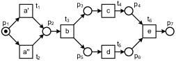
Figure 4. A workflow system.

To give an example, consider the workflow system $S$ in Figure 4. For this system, the expression $\mathit{canOccur(S,\texttt{a}^{\prime})}\land\neg\;\mathit{alwaysOccurs(S,\texttt{a}^{\prime})}$ evaluates to true. Indeed, there exists a label execution $\eta_{1}:=\left\langle\texttt{a}^{\prime},\texttt{b},\texttt{c},\texttt{d},\texttt{e}\right\rangle$ of $S$ that justifies the fact that $\texttt{a}^{\prime}$ can occur in $S$, and a label execution $\eta_{2}:=\left\langle\texttt{a}^{\prime\prime},\texttt{b},\texttt{c},\texttt{d},\texttt{e}\right\rangle$ of $S$ that justifies the fact that $\texttt{a}^{\prime}$ does not always occur in $S$. Note that strings b, c, d, and e, always occur in $S$ as they are present in all of the four label executions of $S$. Furthermore, both $\mathit{canConflict}(S,\texttt{b},\texttt{a}^{\prime})$ and $\mathit{canCooccur}(S,\texttt{b},\texttt{a}^{\prime})$ evaluate to true, because b can be observed without $\texttt{a}^{\prime}$, for example in $\eta_{2}$, and with $\texttt{a}^{\prime}$, for example in $\eta_{1}$. Note that a and $\texttt{a}^{\prime}$ are in conflict, i.e., $\mathit{conflict}(S,\texttt{a},\texttt{a}^{\prime})$ evaluates to true, as these two strings are never observed together. Finally, b and e are example strings that co-occur in $S$, i.e., $\mathit{cooccur}(S,\texttt{b},\texttt{e})$ evaluates to true.

Executions of workflow systems capture orderings of transition occurrences. One can rely on processes to adequately represent causality and concurrency relations on transition occurrences (Goltz and Reisig, 1983).

Definition 4.5 (Process).

A process of a system $S:=(P,T,F,\lambda,M)$ is a 4-tuple $\pi:=(B,E,G,\rho)$, where $B$ is a set of conditions, $E$ is a set of events, $G\subseteq(B\times E)\cup(E\times B)$ is the flow relation, such that $G^{+}$ is irreflexive and $\forall\,b\in B:|\{e\in E\!\divides\!(e,b)\in G\}|\leq 1\;\land\;|\{e\in E\!\divides\!(b,e)\in G\}|\leq 1$, and $\rho:B\cup E\rightarrow P\cup T$ is such that:

• $\rho(B)\subseteq P$ and $\rho(E)\subseteq T$, i.e., $\rho$ preserves the nature of nodes,

• $\forall\,b_{1},b_{2}\in\mathit{Min}(\pi):(b_{1},b_{2})\not\in G^{+}\land(b_{2},b_{1})\not\in G^{+}$, $\forall\,b_{1}\in B\setminus\mathit{Min}(\pi)\exists\,b_{2}\in\mathit{Min}(\pi):(b_{2},b_{1})\!\in G^{+}$, and $\forall p\in P:M(p)=|\rho^{-1}(p)\cap\mathit{Min}(\pi)|$, i.e., $\pi$ starts at $M$, and

• for every event $e\in E$ and for every place $p\in P$ it holds that
  $|\{(p,t)\in F\!\divides\!t=\rho(e)\}|=|\rho^{-1}(p)\cap\bullet{e}\,|$ and $|\{(t,p)\in F\!\divides\!t=\rho(e)\}|=|\rho^{-1}(p)\cap{e\!}\bullet|$,
  i.e., $\rho$ respects the environment of transitions. $\lrcorner$

A process of a Petri net system is an acyclic bipartite graph, in which conditions and events are two disjoint sets of nodes, and a mapping from nodes of the process to nodes of the system. Figure 5 shows three processes of the system in Figure 4. Conditions and events of a process are drawn as places and transitions, respectively. The labels in the figures encode mappings of nodes of processes to nodes of the system. In particular, each condition $b_{i}$ maps to place $p_{i}$, $i\in[1..7]$, and each event $e_{j}$ maps to transition $t_{j}$, $j\in[1..6]$. In general, several conditions (events) of a process can refer to the same place (transition) of the corresponding system. For example, there exist processes of the system in Figure LABEL:fig:system in which several conditions and several events refer to the same place and transition, respectively. These are the processes that describe multiple occurrences of transitions in the loop with entry place $c_{4}$ and exit place $c_{5}$.

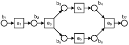
Figure 5. Three processes of the system in Figure 4.

Given a process $\pi$ of a system $S$, by $E_{\pi}$ and $\rho_{\pi}$ we refer to events of $\pi$ and the function that maps nodes of $\pi$ to nodes of $S$, respectively. A process $\pi$ of $S$ can be interpreted as a collection of occurrence sequences of $S$, where every event $e\in E_{\pi}$ describes an occurrence of transition $\rho_{\pi}(e)$. For example, the process in Figure 5 describes a single occurrence sequence of the system in Figure 4, namely $\left\langle t_{1},t_{3},t_{5}\right\rangle$, whereas the process in Figure 5 describes two occurrence sequences of the system in Figure 4, namely $\left\langle t_{1},t_{3},t_{4},t_{5},t_{6}\right\rangle$ and $\left\langle t_{1},t_{3},t_{5},t_{4},t_{6}\right\rangle$. Given a workflow system $S$, by $\Pi_{S}$ we denote the set that contains all and only processes of $S$ (up to isomorphism) that describe all the executions of $S$. Note that the set of all processes of a workflow system can be infinite. For example, the set of all processes of the system in Figure LABEL:fig:system that describe all its executions is infinite. Let $S$ be the workflow system in Figure 4. Then, $\Pi_{S}$ is composed of the two processes shown in Figs. 5 and 5; these two processes describe all the four executions of the system. Note that the process from Figure 5 is not in $\Pi_{S}$ because the occurrence sequence it describes is not an execution of $S$. Finally, by $\Delta_{S}(x,y)$, where $x,y\in\mathbb{C}$, we refer to the set $\{\pi\in\Pi_{S}\!\divides\!\exists\,e_{1},e_{2}\in E_{\pi}:\lambda(\rho_{\pi}(e_{1}))=x\;\land\;\lambda(\rho_{\pi}(e_{2}))=y\}$, i.e., the set that consists of every process from $\Pi_{S}$ which contains an event that describes an occurrence of a transition with label $x$ and an event that describes an occurrence of a transition with label $y$.

Processes of systems can be characterized by the causality and concurrency relations over their nodes (Nielsen et al., 1981; Goltz and Reisig, 1983). An event $e_{1}\in E_{\pi}$ causes event $e_{2}\in E_{\pi}$ of a process $\pi$, denoted by $e_{1}\rightarrowtail_{\pi}e_{2}$, iff $(e_{1},e_{2})\in G^{+}$. Two events $e_{1}\in E_{\pi}$ and $e_{2}\in E_{\pi}$ are concurrent in $\pi$, denoted by $e_{1}\;||_{\pi}\;e_{2}$, iff $(e_{1},e_{2})\not\in G^{+}$ and $(e_{2},e_{1})\not\in G^{+}$. Intuitively, the fact that event $e_{1}$ is a cause for event $e_{2}$ means that one has to observe an occurrence of transition described by $e_{1}$ prior to observing an occurrence of transition described by $e_{2}$. The fact that two events are concurrent means that the corresponding transitions can be enabled simultaneously in some occurrence sequence of the system and be performed one after another in any order. For process $\pi$ in Figure 5 it holds that $e_{2}\rightarrowtail_{\pi}e_{6}$, $e_{3}\rightarrowtail_{\pi}e_{4}$, and $e_{5}\;||_{\pi}\;e_{4}$.

The total causal and total concurrent relations are now defined as follows.

Definition 4.6 (Total causality and total concurrency).

Let $S:=(P,T,F,\lambda,M)$ be a workflow system and let $x,y\in\mathbb{C}$ be two non-empty character strings.

• $x$ and $y$ are total causal in $S$, denoted by $\mathit{totalCausal}(S,x,y)$, iff 
  $\forall\,\pi\in\Delta_{S}(x,y)\;\forall\,e_{1}\in E_{\pi}\;\forall\,e_{2}\in E_{\pi}:(e_{1}\neq e_{2}\;\land\;\lambda(\rho_{\pi}(e_{1}))=x\;\land\;\lambda(\rho_{\pi}(e_{2}))=y)\Rightarrow e_{1}\;\rightarrowtail_{\pi}\;e_{2}$.

• $x$ and $y$ are total concurrent in $S$, denoted by $\mathit{totalConcurrent}(S,x,y)$, iff 
  $\forall\,\pi\in\Delta_{S}(x,y)\;\forall\,e_{1}\in E_{\pi}\;\forall\,e_{2}\in E_{\pi}:(e_{1}\neq e_{2}\;\land\;\lambda(\rho_{\pi}(e_{1}))=x\;\land\;\lambda(\rho_{\pi}(e_{2}))=y)\Rightarrow e_{1}\;||_{\pi}\;e_{2}$. $\lrcorner$

For example, $\mathit{totalCausal(S,\texttt{a}^{\prime},\texttt{c})}$ holds for workflow system $S$ in Figure 4; in every execution of $S$ in which $\texttt{a}^{\prime}$ and c both occur it holds that every occurrence of $\texttt{a}^{\prime}$ precedes every occurrence of c. As another example, $\mathit{totalConcurrent(S,\texttt{c},\texttt{d})}$ holds for the same system.

Predicates over PQL tasks. Next, we lift the PQL predicates from individual labels to PQL tasks, i.e., to sets of character strings. To this end, we employ the label unification principle proposed in (Polyvyanyy et al., 2014b). Given a system $S$ and a character string $x\in\mathbb{C}$, label unification of $x$ in $S$ is a transformation of $S$ into a fresh system $S^{\prime}$ that is behaviorally equivalent to $S$ but in which every occurrence of $x$ is guaranteed to be triggered by a (fresh) dedicated transition, refer to Definition 6.2 and Lemma 6.5 in (Polyvyanyy et al., 2014b). Let $X$ be the set of all transitions of $S$ that have label $x$ such that $|X|>1$. The label unification of $x$ in $S$ augments $S$ to result in a system $S^{\prime}$ that is behaviorally equivalent to $S$ but ‘forbids’ occurrences of transitions in $X$ and ensures that tokens from the input places of transitions in $X$ are ‘rerouted’ to the only input place of the dedicated transition $\hat{t}$ that has label $x$. Note that if $X$ is a singleton, then all occurrences of $x$ generated by $S$ are guaranteed to be triggered by transition $t\in X$ and, hence, there is no need to transform $S$, i.e., it holds that $S^{\prime}=S$.

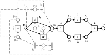
Figure 6. A system obtained via unification of the set of labels $\{\texttt{a},\texttt{a}^{\prime}\}$ in the workflow system in Figure 4.

The concept of a PQL task is introduced in the language to allow handling several distinct labels as if they all represent the same activity. For example, two character strings $\texttt{a}^{\prime}:=$“process payment by cash” and $\texttt{a}^{\prime\prime}:=$“process payment by check” may be seen as sufficiently similar to represent activity $\texttt{a}:=$“process payment”. PQL adapts the label unification principle to operationalize the above sketched intuition. Figure 6 shows the result of performing label unification for labels $\texttt{a}^{\prime}$ and $\texttt{a}^{\prime\prime}$ in the system in Figure 4. The fresh elements introduced during the unification are highlighted in gray, while the fresh arcs, in addition, are depicted using the dashed lines. Unlike in the system in Figure 4, transitions with labels $\texttt{a}^{\prime}$ and $\texttt{a}^{\prime\prime}$ cannot occur in executions of the system in Figure 6. However, in the transformed system, the tokens from the input places of the “forbidden” transitions $t_{1}$ and $t_{2}$ can be rerouted to enable the fresh transition $\hat{t}$ that has label a and can occur instead of both forbidden transitions; transition $\hat{t}$ is called the solitary transition for labels $\texttt{a}^{\prime}$ and $\texttt{a}^{\prime\prime}$.

By $\mathit{unify}(S,X)$, $X\in\powerset_{\geq 1}{(\mathbb{C})}$, we denote the result of the adapted label unification of $X$ in $S$. This result is a pair $(S^{\prime},\hat{t})$, where $S^{\prime}$ is the transformed system and $\hat{t}$ is the fresh solitary transition for labels in $X$. For example, it holds that $\mathit{unify}(S,X)=(S^{\prime},\hat{t})$, where $S$ is the system in Figure 4, $S^{\prime}$ is the system in Figure 6, and $X=\{\texttt{a}^{\prime},\texttt{a}^{\prime\prime}\}$.

It is easy to see that the order of applying different label unifications has no impact on the resulting system as long as fresh solitary transitions have unique labels. Finally, the predicates over PQL tasks are defined as follows.

Definition 4.7 (Predicates over PQL tasks).

Let $S:=(P,T,F,\lambda,M)$ be a workflow system and let $X,Y\in\powerset_{\geq 1}{(\mathbb{C})}$ be two non-empty sets of non-empty character strings.

• $X$ can occur in $S$, denoted by $\mathit{canOccur}(S,X)$, iff 
  it holds that $\mathit{canOccur}(S^{\prime},x)$, where $\mathit{unify}(S,X)=(S^{\prime},x)$.

• $X$ always occurs in $S$, denoted by $\mathit{alwaysOccurs}(S,X)$, iff 
  it holds that $\mathit{alwaysOccurs}(S^{\prime},x)$, where $\mathit{unify}(S,X)=(S^{\prime},x)$.

• $X$ can conflict with $Y$ in $S$, denoted by $\mathit{canConflict}(S,X,Y)$, iff it holds that $\mathit{canConflict}(S^{\prime\prime}\!,x,y)$, where $\mathit{unify}(S,X)=(S^{\prime},x)$ and $\mathit{unify}(S^{\prime},Y)=(S^{\prime\prime}\!,y)$.

• $X$ and $Y$ can co-occur in $S$, denoted by $\mathit{canCooccur}(S,X,Y)$, iff it holds that $\mathit{canCooccur}(S^{\prime\prime}\!,x,y)$, where $\mathit{unify}(S,X)=(S^{\prime},x)$ and $\mathit{unify}(S^{\prime},Y)=(S^{\prime\prime}\!,y)$.

• $X$ and $Y$ are in conflict in $S$, denoted by $\mathit{conflict}(S,X,Y)$, iff 
  it holds that $\mathit{conflict}(S^{\prime\prime}\!,x,y)$, where $\mathit{unify}(S,X)=(S^{\prime},x)$ and $\mathit{unify}(S^{\prime},Y)=(S^{\prime\prime}\!,y)$.

• $X$ and $Y$ co-occur in $S$, denoted by $\mathit{cooccur}(S,X,Y)$, iff 
  it holds that $\mathit{cooccur}(S^{\prime\prime}\!,x,y)$, where $\mathit{unify}(S,X)=(S^{\prime},x)$ and $\mathit{unify}(S^{\prime},Y)=(S^{\prime\prime}\!,y)$.

• $X$ and $Y$ are total causal in $S$, denoted by $\mathit{totalCausal}(S,X,Y)$, iff 
  it holds that $\mathit{totalCausal}(S^{\prime\prime}\!,x,y)$, where $\mathit{unify}(S,X)=(S^{\prime},x)$ and $\mathit{unify}(S^{\prime},Y)=(S^{\prime\prime}\!,y)$.

• $X$ and $Y$ are total concurrent in $S$, denoted by $\mathit{totalConcurrent}(S,X,Y)$, iff 
  it holds that $\mathit{totalConcurrent}(S^{\prime\prime}\!,x,y)$, where $\mathit{unify}(S,X)=(S^{\prime},x)$ and $\mathit{unify}(S^{\prime},Y)=(S^{\prime\prime}\!,y)$. $\lrcorner$

Using the proposed denotations, one can verify that, for instance, $\mathit{alwaysOccurs}(S,\{\texttt{a}^{\prime},\texttt{a}^{\prime\prime}\})$ evaluates to true, where $S$ is the system in Figure 4. Hence, for example, one can retrieve the system in Figure 4 by issuing the query “SELECT * FROM * WHERE AlwaysOccurs($\sim$a);”, given that $\sim$a evaluates to $\{\texttt{a}^{\prime},\texttt{a}^{\prime\prime}\}$. One can use queries like the one exemplified to perform exploratory querying or address the problem of the inconsistent usage of labels in process repositories, where label a from the user specified query gets replaced by labels $\texttt{a}^{\prime}$ and $\texttt{a}^{\prime\prime}$ from the process repository.

4.6.2. Computations of the PQL Predicates

Definition 4.7 specifies the eight selected predicates over PQL tasks in terms of the corresponding predicates over transitions. The reader can find techniques to compute the $\mathit{canConflict}$, $\mathit{canCooccur}$, and $\mathit{totalCausal}$ predicates over transitions in (Polyvyanyy et al., 2014b). Using $\mathit{canConflict}$ and $\mathit{canCooccur}$, one can compute the $\mathit{conflict}$ and $\mathit{cooccur}$ predicates, refer to Definition 4.7. Next, we propose techniques that given a sound workflow system $S:=(P,T,F,\lambda,M)$ compute whether $t\in T$ can occur in $S$, $t\in T$ always occurs in $S$, and $t_{1}\in T$ and $t_{2}\in T$ are total concurrent in $S$. PQL performs these computations on systems obtained via unifications of sets of labels, refer to Section 4.6.1 and (Polyvyanyy et al., 2014b) for details. Note that label unification in a sound workflow system often leads to a system that is not even a workflow system; due to the introduction of dead transitions, where a dead transition is a transition which is not part of any occurrence sequence of the system; see for example transitions $t_{1}$ and $t_{2}$ in Figure 6. Dead transitions are kept in the resulting systems as they may be required to perform subsequent transformations. However, once all the transformations are applied, dead transitions can be removed from the system to result in a sound workflow system; this trivially follows from the definition of label unification. Note that in what follows, we restrict some discussions to sound workflow systems.

Can occur transition. One can check whether a transition can occur in a workflow system by solving a reachability problem on a transformed version of the system.

Definition 4.8 (Can occur transition).

A transition $t\in T$ can occur in a workflow system $S:=(P,T,F,\lambda,M)$ iff there exists an execution $\sigma$ of $S$ such that $t\in\sigma$. $\lrcorner$

Given a system and marking, the reachability problem consists of deciding if there is an occurrence sequence of the system that leads to the marking. Note that the reachability problem is decidable (Hack, 1975).

Lemma 4.9 (Can occur transition).

Let $S:=(P,T,F,\lambda,M)$ be a workflow system with a sink place $o\in P$. A transition $t\in T$ can occur in $S$ iff there exists an occurrence sequence $\sigma$ of $S^{\prime}:=(P\cup\{p^{\prime}\},T\cup\{t^{\prime}\},F\cup\{(p^{\prime},t^{\prime})\}\cup\{(p,t^{\prime})\!\divides\!p\in\bullet{t}\}\cup\{(t^{\prime},p)\!\divides\!p\in{t}\bullet\},\lambda\cup\{(t^{\prime},\epsilon)\},M\cupplus[p^{\prime}])$, where $p^{\prime}\not\in P$ and $t^{\prime}\not\in T$ are a fresh place and transition, respectively, such that $t^{\prime}$ is an element of $\sigma$, i.e., $t^{\prime}\in\sigma$, and $\sigma$ leads to $[o]$. $\lrcorner$

The proof of Lemma 4.9 is straightforward due to the construction of $S^{\prime}$. If $t$ can occur in $S$, then there exists an execution $\gamma$ of $S$ that contains $t$ at some position $j$ of $\gamma$. A sequence of transitions obtained from $\gamma$ by replacing $t$ at position $j$ with $t^{\prime}$ is an occurrence sequence of $S^{\prime}$ that leads to $[o]$. Let $\sigma$ be an occurrence sequence of $S^{\prime}$ that leads to $[o]$ and $t^{\prime}\in\sigma$. Then, a sequence of transitions obtained from $\sigma$ by replacing $t^{\prime}$ with $t$ and keeping the order of the remaining elements is an execution of $S$; note that $\sigma$ contains exactly one occurrence of $t^{\prime}$.

Always occurs transition. Next, we present a technique for checking whether a transition always occurs in a sound workflow system.

Definition 4.10 (Always occurs transition).

A transition $t\in T$ always occurs in a sound workflow system $S:=(P,T,F,\lambda,M)$ iff for every execution $\sigma$ of $S$ it holds that $t\in\sigma$. $\lrcorner$

One can check whether a transition always occurs in a sound workflow system by solving a reachability problem on a transformed version of the system.

Lemma 4.11 (Always occurs transition).

Let $S:=(P,T,F,\lambda,M)$ be a workflow system with a sink place $o\in P$. A transition $t\in T$ always occurs in $S$ iff there exists no occurrence sequence $\sigma$ of $S^{\prime}:=(P\cup\{p^{\prime}\},T,F\cup\{(p^{\prime},t)\},\lambda,M\cupplus[p^{\prime}])$, where $p^{\prime}\not\in P$ is a fresh place, that leads to $[p^{\prime},o]$. $\lrcorner$

The proof of Lemma 4.11 is straightforward due to the construction of $S^{\prime}$. If $t$ always occurs in $S$, then every execution of $S$ contains $t$. Let $\gamma$ be an execution of $S$ without $t$, then $\gamma$ is an occurrence sequence of $S^{\prime}$ that leads to $[p^{\prime},o]$. Finally, let $\sigma$ be an occurrence sequence of $S^{\prime}$ that leads to $[p^{\prime},o]$. Then, clearly, $\sigma$ is an execution of $S$ without $t$.

Total concurrent transitions. Let $S:=(P,T,F,\lambda,M)$ be a workflow system. By $\Xi_{S}(t_{1},t_{2})$, where $t_{1},t_{2}\in T$, we denote the set $\{\pi\in\Pi_{S}\!\divides\!\exists\,e_{1},e_{2}\in E_{\pi}:\rho_{\pi}(e_{1})=t_{1}\;\land\;\rho_{\pi}(e_{2})=t_{2}\}$.

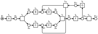
Figure 7. A workflow system.

Definition 4.12 (Total concurrent transitions).

Transitions $t_{1}\in T$ and $t_{2}\in T$ are total concurrent in a sound workflow system $S:=(P,T,F,\lambda,M)$ iff $\forall\,\pi\in\Xi_{S}(t_{1},t_{2})\;\forall\,e_{1}\in E_{\pi}\;\forall\,e_{2}\in E_{\pi}:(e_{1}\neq e_{2}\;\land\;\rho_{\pi}(e_{1})=t_{1}\;\land\;\rho_{\pi}(e_{2})=t_{2})\Rightarrow e_{1}\;||_{\pi}\;e_{2}$. $\lrcorner$

The unfolding of a Petri net system is an acyclic graph that encodes all the processes of the system in a possibly infinite, tree-like structure (McMillan, 1992; Esparza et al., 2002). In (McMillan, 1992), McMillan proposed an algorithm for constructing a finite initial part of the unfolding, called a complete prefix of the unfolding, which contains full information about the behavior of the system, i.e., all the processes of the system.

Figure 7 shows a workflow system $S$ obtained by translating the process model shown later in Figure 9 (model 9), refer to Section 4.7, into a Petri net system. Figure 8 shows a complete prefix of the unfolding $U$ of $S$. A complete prefix of the unfolding of a system $S:=(P,T,F,\lambda,M)$ is a 4-tuple $U:=(B,E,G,\rho)$, where $B$ and $E$ are disjoint sets of conditions and events, respectively, $G\subseteq(B\times E)\cup(E\times B)$ is the flow relation, such that $G^{+}$ is irreflexive, and $\rho:B\cup E\rightarrow P\cup T$ is a function that maps conditions to places and events to transitions. Thus, a complete prefix of the unfolding is a process that allows forward conflicts (McMillan, 1992).

Figure 8. A complete prefix of the unfolding of the system in Figure 7.

In Figure 8, conditions and events are shown as circles and rectangles, respectively. Every condition $b_{i},b^{\prime}_{i},\ldots$ represents one token at place $p_{i}$, $i\in\mathbb{N}$, refer to (Polyvyanyy et al., 2015b). Every event $e_{j},e^{\prime}_{j},\ldots$ represents one occurrence of transition $t_{j}$, $j\in\mathbb{N}$. McMillan proposes to associate every event $e$ of a compete prefix of the unfolding of a Petri net system with a marking that one reaches by firing all the transitions encoded by the events in the local configuration of $e$. The local configuration of an event $e$, denoted by $\left\lceil e\right\rceil$, is the set of events composed of $e$, all the events from which there is a directed path to $e$, and no other events. For example, $\left\lceil e_{4}\right\rceil=\{e_{1},e_{2},e_{3},e_{4}\}$ and $\left\lceil e_{7}\right\rceil=\{e_{1},e_{2},e_{3},e_{4},e_{5},e_{6},e_{7}\}$. One reaches the marking $[p_{5},p_{6}]$ by firing transitions represented by the events in $\left\lceil e_{4}\right\rceil$, and the marking $[p_{9}]$ by firing transitions represented by the events in $\left\lceil e_{7}\right\rceil$. These markings are encoded by the sets of conditions $\{b_{5},b_{6}\}$ and $\{b_{9}\}$ in Figure 8, respectively, and are denoted by $\mathit{Cut}(\left\lceil e_{4}\right\rceil)$ and $\mathit{Cut}(\left\lceil e_{7}\right\rceil)$, respectively. Note that the marking $[p_{9}]$ can also be reached in the system in Figure 7 after occurrences of transitions encoded by the events in the local configuration of event $e^{\prime}_{7}$.

Intuitively, if one continues constructing the prefix in Figure 8, the part that will follow $\mathit{Cut}(\left\lceil e^{\prime}_{7}\right\rceil)$ will be isomorphic to the part of the prefix that will follow $\mathit{Cut}(\left\lceil e_{7}\right\rceil)$. Hence, McMillan proposed to stop the construction at $\mathit{Cut}(\left\lceil e^{\prime}_{7}\right\rceil)$ and refers to $e^{\prime}_{7}$ and $e_{7}$ as a cutoff and its corresponding event, respectively. We denote the set of all the cutoff events of a complete prefix of the unfolding $U$ by $\mathit{cutoffs}(U)$. Given a cutoff event $e$, by $\mathit{corr}(e)$, we denote the corresponding event of $e$. Thus, $\mathit{cutoffs}(U)$, where $U$ is a complete prefix of the unfolding in Figure 8, is equal to $\{e^{\prime}_{7}\}$, and $\mathit{corr}(e^{\prime}_{7})=e_{7}$. In the figure, the relation between the cutoff and its corresponding event is shown by the dotted arrow. For further details on (complete prefixes of) the unfoldings please refer to (McMillan, 1992; Esparza et al., 2002).

Let $U:=(B,E,G,\rho)$ be a complete prefix of the unfolding of a system $S:=(P,T,F,\lambda,M)$. Then, it holds that $\mathit{path}(U,e_{1},e_{2})$ iff $(e_{1},e_{2})\in G^{+}$, or $(e_{2},e_{1})\in G^{+}$, or there exists a sequence of cutoffs $c\in\mathit{cutoffs}(U)^{*}$ such that (i) $\exists\,b\in\mathit{Cut}(\left\lceil c_{1}\right\rceil):(e_{1},b)\in G^{+}$, (ii) $\exists\,b\in\mathit{Cut}(\left\lceil\mathit{corr}(c_{|c|})\right\rceil):(b,e_{2})\in G^{+}$, and (iii) $\forall\,i\in[1..(|c|-1)]\exists\,b_{1}\in\mathit{Cut}(\left\lceil\mathit{corr}(c_{i})\right\rceil)\exists\,b_{2}\in\mathit{Cut}(\left\lceil c_{i+1}\right\rceil):(b_{1},b_{2})\in G^{*}$.

Lemma 4.13 (Total concurrent transitions).

Let $S:=(P,T,F,\lambda,M)$ be a sound workflow system and let $U:=(B,E,G,\rho)$ be a complete prefix of the unfolding of $S$. Transitions $t_{1}\in T$ and $t_{2}\in T$ are total concurrent in $S$ iff $\forall e_{1}\!\in E\,\forall e_{2}\!\in E:(e_{1}\neq e_{2}\;\land\;\rho(e_{1})=t_{1}\;\land\;\rho(e_{2})=t_{2})\Rightarrow\neg\;\mathit{path}(U,e_{1},e_{2})$. $\lrcorner$

Let us assume that $t_{1}$ and $t_{2}$ are total concurrent in $S$ and there exist two distinct events $e_{1}$ and $e_{2}$ that describe occurrences of $t_{1}$ and $t_{2}$, respectively, such that $\mathit{path}(U,e_{1},e_{2})$. Then, there is a process in $\Xi_{S}(t_{1},t_{2})$ that contains two distinct causal events that refer to $t_{1}$ and $t_{2}$. This follows immediately from the definition of a complete prefix of the unfolding, cf. (Esparza et al., 2002), and the fact that every occurrence sequence of $S$ can be extended to an execution. If for every two distinct events $e_{1}$ and $e_{2}$ that describe occurrences of $t_{1}$ and $t_{2}$ it holds that $\neg\,\mathit{path}(U,e_{1},e_{2})$, then $t_{1}$ and $t_{2}$ are total concurrent in $S$, as according to the definition of a complete prefix of the unfolding there exists no process in $\Xi_{S}(t_{1},t_{2})$ that evidences that some occurrences of $t_{1}$ and $t_{2}$ are causal.

Note that one can always construct a complete prefix of the unfolding of a bounded system (Esparza et al., 2002), i.e., a system with a finite number of reachable states, while a sound workflow system is guaranteed to be bounded (van der Aalst, 1997). Using the prefix in Figure 8 and Lemma 4.13 one can verify whether two given transitions are total concurrent in the system $S$ in Figure 7. For example, transitions $t_{3}$ and $t_{5}$ are total concurrent in $S$. Transitions $t_{3}$ and $t_{6}$ are not total concurrent in $S$ because of events $e_{3}$ and $e^{\prime}_{6}$ and the fact that $(e_{3},e^{\prime}_{6})\in G^{+}$. Transitions $t_{9}$ and $t_{11}$ are also not total concurrent in $S$ because of events $e_{9}$ and $e_{11}$ and the sequence of cutoff events $\left\langle e^{\prime}_{7}\right\rangle$; note that $(e_{9},b^{\prime}_{9})\in G^{+}$ and $(b_{9},e_{11})\in G^{+}$.

4.7. Sample PQL Queries

We now consider an example process repository consisting of ten process models that are sourced from the collection of the SAP R/3 reference model (Curran et al., 1998) as well as from Polyvyanyy’s PhD thesis (Polyvyanyy, 2012). Figure 9 depicts the ten process models using BPMN. In a BPMN model, activities are used to model tasks and are drawn as rectangles. Gateways are visualized as diamonds. Exclusive gateways use a marker which is shaped like “$\times$” inside the diamond shape, wheres parallel gateways use a marker which is shaped like “$+$” inside the diamond shape. Directed arcs encode control flow dependencies. For simplicity, the models in Figure 9 use only abstract task labels (which are alphabet letters). In addition, the attributes information of each process model, including its ID, version, date created, and author, is shown in the text annotation under the model.

The example process model repository discussed in this section can be formalized as the 6-tuple $(S,A,L,\mathit{val},\mathit{loc},\precsim)$, refer to Definition 4.1, where $S$ is the set of ten Petri net systems $\{s_{1},\ldots,s_{10}\}$, $s_{i}$, $i\in\{1..10\}$, captures the behavior of model $i$ in Figure 9; the corresponding net systems can be obtained from BPMN models using the approach from (Dijkman et al., 2008), $A:=$ {ID, Version, Date, Author} is the set of attribute names, $L:=\{/,\,\,/\texttt{Ten-Models-BPMN},\,\,/\texttt{SAP-R3-EPC-Repo}\}$ is the set of locations, $\mathit{val}:=$ {($s_{1}$, ID, 1), ($s_{1}$, Version, 1.0), ($s_{1}$, Date, 01-June-2017), $\ldots$} is the attribute value assignment function, $\mathit{loc}:=\cup_{i\in\{1..10\}}(s_{i},/\texttt{Ten-Models-BPMN})$ is the location assignment function, and $\precsim$ is the location map such that $(l,l)\in\,\,\precsim$ for every $l\in L$, and $(/\texttt{Ten-Models-BPMN},/)\in\,\,\precsim$ and $(/\texttt{SAP-R3-EPC-Repo},/)\in\,\,\precsim$.

Figure 9. A repository of ten process models (in BPMN) with their attributes information and results of evaluation of ten sample queries over each of these models.

The process models in Figure 9 have various structural features and are sound. The first five models (models 1 to 5) capture acyclic processes and the other five (models 6 to 10) specify processes that contain cycles. Models 1, 2, 6, and 10 are well-structured, where a process model is well-structured if and only if every node with multiple outgoing arcs (a split) has a corresponding node with multiple incoming arcs (a join), and vice versa, such that the set of nodes between the split and the join induces a SESE component (Polyvyanyy et al., 2010); otherwise the model is said to be unstructured (Polyvyanyy, 2012). Models 3, 4, 5, 7, 8, and 9 in Figure 9 are unstructured. Model 7, 8, and 9 can be mapped to well-structured models. For example, model 10 is equivalent to model 9 and is well-structured. Note that models 3 to 5 are inherently unstructured, i.e., the behaviors they describe do not have equivalent well-structured representations (if the concurrency relations between process tasks must be preserved) (Polyvyanyy, 2012). Among these models, model 4 has a typical Z-structure (Kiepuszewski et al., 2000), which is formed by the control flow dependencies between tasks $A$, $B$, $C$, and $D$.

Next, we propose ten sample queries:

• SELECT "Author" FROM "/Ten-Models-BPMN"

• WHERE CanOccur("D") AND Conflict("D","E");
  

• SELECT "Version" FROM "/Ten-Models-BPMN"

• WHERE AlwaysOccurs("C") OR Cooccur("B","C");
  

• SELECT "Date" FROM "/Ten-Models-BPMN"

• WHERE (CanOccur("G") AND (NOT Conflict("E","G"))) OR 

• (TotalConcurrent("C","D") AND AlwaysOccurs("D"));
  

• SELECT "Author","Version" FROM "/Ten-Models-BPMN"

• WHERE CanOccur({"F","G"},ALL) AND AlwaysOccurs({"F","G"},ANY);
  

• SELECT "Version","Date" FROM "/Ten-Models-BPMN"

• WHERE Cooccur("B",{"C","D"},ALL) AND TotalConcurrent("B",{"C","D"},ANY);
  

• SELECT "Version","Author" FROM "/Ten-Models-BPMN"

• WHERE Conflict({"A","B"},{"E","F"},ANY) OR 

• (Cooccur({"A","B"},{"E","F"},EACH) AND 

• TotalCausal({"A","B"},{"E","F"},ALL));
  

• SELECT "Date","Author" FROM "/Ten-Models-BPMN"

• WHERE "C" IN (GetTasksAlwaysOccurs({"C"}) UNION 

• GetTasksTotalCausal({"C"},{"B","D"},ALL));
  

• SELECT "Date","Version" FROM "/Ten-Models-BPMN"

• WHERE "G" IN (GetTasksCanOccur({"G"}) INTERSECT 

• GetTasksConflict({"G"},{"D","E","F"},ANY));
  

• SELECT "Version","Date","Author" FROM "/Ten-Models-BPMN"

• WHERE GetTasksCooccur({"A","B","C"},{"D","E"},ANY) NOT EQUALS 

• GetTasksTotalConcurrent({"A","B","C"},{"D","E"},ANY);
  

• SELECT * FROM "/Ten-Models-BPMN" WHERE ({"A","B","E","F"} EXCEPT 

• GetTasksCooccur({"A","B","E","F"},{"C","D"},ALL)) OVERLAPS WITH 

• GetTasksConflict({"A","B","E","F"},{"C","D"},ANY);

The PQL constructs used to specify these queries include the atomic behavioral predicates, the corresponding predicate macros, logical operations (over predicates and predicate macros), construction of task sets using predicates, set operations, and set comparison operations. Note that these sample queries (named Q1–Q10), are instantiations of ten query templates (out of a total of 150 query templates listed in Appendix C) to be used for evaluation of PQL in Section 6.1.

We executed the above ten queries on the repository of ten process models shown in Figure 9. Each query was evaluated over each of these ten process models according to the semantics of PQL (defined in Sections 4.5 and 4.6). The evaluation result indicates whether a process model satisfies the condition specified in the WHERE clause of a specific query. In Figure 9, this is depicted by a query name being ticked or not ticked under each process model. Note that since models 9 and 10 are behaviorally equivalent, every query evaluation over these models yields the same result.

Table 6. Answers to ten sample queries over the repository of ten process models in Figure 9.

Query	Query result
Q1	{($s_{1}$,{(Author, SAP)}), ($s_{5}$,{(Author, Polyvyanyy)})}
Q2	{($s_{1}$,{(Version, 1.0)}), ($s_{4}$,{(Version, 1.2)}), ($s_{6}$,{(Version, 2.0)}), ($s_{7}$,{(Version, 1.2)}),
	($s_{9}$,{(Version, 1.2)}), ($s_{10}$,{(Version, 2.0)})}
Q3	{($s_{4}$,{(Date, 31-May-2017)}), ($s_{6}$, {(Date, 01-June-2017)}), ($s_{7}$,{(Date, 01-June-2017)}),
	($s_{9}$,{(Date, 05-June-2017)}), ($s_{10}$,{(Date, 05-June-2017)})}
Q4	{($s_{6}$,{(Author, SAP), (Version, 2.0)}), ($s_{9}$,{(Author, Polyvyanyy), (Version, 1.2)}),
	($s_{10}$,{(Author, Polyvyanyy), (Version, 2.0)})}
Q5	{($s_{4}$,{(Version, 1.2), (Date, 31-May-2017)}), ($s_{9}$,{(Version, 1.2), (Date, 05-June-2017)}),
	($s_{10}$,{(Version, 2.0), (Date, 05-June-2017)})}
Q6	{($s_{1}$,{(Version, 1.0), (Author, SAP)}), ($s_{2}$,{(Version, 1.1), (Author, SAP)}),
	($s_{3}$,{(Version, 2.0), (Author, Polyvyanyy)})}
Q7	{($s_{1}$,{(Date, 01-June-2017), (Author, SAP)}), ($s_{2}$,{(Date, 31-May-2017), (Author, SAP)}),
	($s_{3}$,{(Date, 03-June-2017), (Author, Polyvyanyy)}), ($s_{4}$,{(Date, 31-May-2017), (Author, SAP)}),
	($s_{7}$,{(Date, 01-June-2017), (Author, SAP)}), ($s_{9}$,{(Date, 05-June-2017), (Author, Polyvyanyy)}),
	($s_{10}$,{(Date, 05-June-2017), (Author, Polyvyanyy)})}
Q8	{($s_{8}$, {(Date, 03-June-2017), (Version, 2.0)})}
Q9	{($s_{3}$,{(Version, 2.0), (Date, 03-June-2017), (Author, Polyvyanyy)}), ($s_{4}$,{(Version, 1.2),
	(Date, 31-May-2017), (Author, SAP)}), ($s_{5}$,{(Version, 1.2), (Date, 03-June-2017),
	(Author, Polyvyanyy)}), ($s_{6}$,{(Version, 2.0), (Date, 01-June-2017), (Author, SAP)}),
	($s_{7}$,{(Version, 1.2), (Date, 01-June-2017), (Author, SAP)}), ($s_{9}$,{(Version, 1.2),
	(Date, 05-June-2017), (Author, Polyvyanyy)}), ($s_{10}$,{(Version, 2.0),
	(Date, 05-June-2017), (Author, Polyvyanyy)})}
Q10	{($s_{1}$,{(ID, 1), (Version, 1.0), (Date, 01-June-2017), (Author, SAP)}), ($s_{2}$,{(ID, 2), (Version, 1.1),
	(Date, 31-May-2017), (Author, SAP)}), ($s_{3}$,{(ID, 3), (Version, 2.0), (Date, 03-June-2017),
	(Author, Polyvyanyy)}), ($s_{5}$,{(ID, 5), (Version, 1.2), (Date, 03-June-2017), (Author, Polyvyanyy)}),
	($s_{6}$,{(ID, 6), (Version, 2.0), (Date, 01-June-2017), (Author, SAP)})}

Table 6 summarizes the results of executing the ten sample queries. For each query, only the corresponding systems (and their attributes) that satisfy the WHERE condition of the query are retrieved. For example, Query Q1 is designed to retrieve those process models where (i) task labeled "D" (task D for short) occurs in at least one process instance (CanOccur("D")) and (ii) there is no process instance in which tasks D and E both occur (Conflict("D","E")). The first condition holds in all models in Figure 9, while the second condition holds in models 1 and 5 only. It is important to understand the behavior of a process model when evaluating the second condition. For example, in model 8, although tasks D and E are on two exclusive branches (subsequent to task B), both tasks may occur in one process instance since task D is part of a cycle. Another interesting example concerns query Q3, in particular, the condition TotalConcurrent("C","D") in the query. This condition holds for a process model if and only if for every instance in which tasks C and D both occur every occurrence of task C can be executed at the same time with every occurrence of task D. For example, due to the characteristics of model 3, i.e., it is unstructured, it is hard to evaluate this condition without knowledge of the model’s behavior.

5. Implementation

The proposed in the previous section querying method has been implemented and is publicly available. The implementation exhibits a well-defined application programming interface (API) to facilitate its integration with other software products. This API can be accessed by the users via command-line interfaces (CLIs) of two utilities: the PQL bot and the PQL tool. We refer to them as PQL Tools and, conjointly, they implement the PQL environment. The PQL bot is used to prepare models for querying, while the PQL tool is used to execute PQL queries over the indexed models.

The PQL environment is implemented using Java, ANTLR, and MySQL technologies. The Java language is chosen due to its “architecture-neutral and portable” principle. As a result, the environment can be deployed on various platforms running different operating systems. The PQL tool uses an ANTLR (Parr, 2013) generated parser that can build and walk syntax trees of PQL queries. Given a context-free grammar expressed using extended Backus-Naur Form (Hopcroft et al., 2006) as input, ANTLR automatically generates Java code of a parser of the grammar. The PQL grammar, which incorporates both the abstract and concrete syntax proposed in Section 4.3 and Section 4.4, respectively, captured using ANTLR notation is listed in Appendix B. To improve execution times of PQL queries, the PQL tool relies on an index of behavioral relations—a special data structure that improves the computation speed of behavioral relations at the cost of time for its construction and space for its storage. The tool uses this index at runtime to avoid having to freshly compute PQL predicates every time a new query is issued. The index is stored in a MySQL relational database system.

The two PQL utilities load their configuration parameters from the global initialization file. These parameters set values to configure database connections, a path to a model checker used by PQL bots, configuration parameters of an information retrieval engine for assessment of label similarities, the default and indexed label similarity thresholds, the maximum number of threads used by the PQL tool when executing queries, the time that PQL bots sleep (i.e., stay idle) between two subsequent indexing jobs, and the maximal allowed time to index a single model. It is easy to configure the PQL environment to use any third-party tool for scoring label similarities, to fulfill the process querying requirements. At the moment, one can configure the PQL environment to use one of the three integrated information retrieval engines to be used when scoring label similarities. These are Apache Lucene, Themis-IR (Polyvyanyy, 2007), and an implementation of the label similarity scoring approach based on the Levenshtein distance. The Apache Lucene and Themis-IR engines are configured to use the vector space model to perform label similarity assessments, while the approach based on the Levenshtein distance is implemented based on the principles proposed in (Li and Liu, 2007).

The PQL bot and the PQL tool are discussed in Section 5.1 and Section 5.2, respectively. Section 5.3 is devoted to the discussion of the integration of the PQL environment with Apromore—an open source process model repository (La Rosa et al., 2011).

5.1. The PQL Bot

The PQL bot is a standalone utility that can be used to systematically index models stored by the PQL tool. Once a model is indexed, it can be matched to a query. One can start multiple PQL bot instances simultaneously to index multiple models in parallel. To construct an index, a PQL bot instance computes all the behavioral predicates over all the PQL tasks of the model and stores them in the database. A call to the PQL indexing routine takes a workflow system described in the Petri Net Markup Language (PNML) format as input. The PNML format is an XML-based syntax for high-level Petri nets, which has been designed as a standard interchange format aimed at enabling Petri net tools to exchange Petri net models (Billington et al., 2003). For many high-level process modeling languages, such as WS-BPEL, EPC, and BPMN, there exist mappings to the Petri net formalism. As a result, the PQL environment can work with models developed using a wide range of modeling tools captured using many mainstream notations. For more information on Petri nets and workflow systems refer to Section 3.2. This section also summarizes the technique for translating process models into workflow systems that was used in the reported implementation of the PQL bot; it is the technique for converting the EPC in Figure LABEL:fig:EPC into the workflow system in Figure LABEL:fig:system.

When initializing a PQL bot instance one can configure it via CLI. Some options of the PQL bot CLI are listed in Table 7. Every PQL bot instance has a unique name, which can be assigned using option -n. If this option is not used, a random unique name is assigned. Once started, a PQL bot instance indexes stored (but not yet indexed) models in succession. One can use CLI options -s and -i to specify time to sleep, i.e., to stay idle, between two successive indexing tasks, and the maximal time to attempt indexing of a model. If these options are not used, the parameters get configured based on the values in the global configuration file. If indexing of a model could not be completed within the given time frame, the model is marked as such that can not be indexed using this version of the bot, and the bot proceeds with indexing the next model. The -h and -v CLI options, respectively, print the help message and get the version of the invoked PQL bot instance.

Table 7. CLI options of the PQL bot.

Option	Option (short)	Parameter	Description
--help	-h		Print help message
--index	-i	<number>	Maximal indexing time (in seconds)
--name	-n	<string>	Name of this bot (maximum 36 characters)
--sleep	-s	<number>	Time to sleep between indexing jobs (in seconds)
--version	-v		Get version of this bot

Once started, a PQL bot instance run as a daemon, i.e., a background process, until it is shut down. An example of the command line output of a PQL bot instance is listed below.

>> java -jar PQL.BOT-1.0.jar -n=Brisbane -s=60 -i=86400
>> =======================================================================
>> Process Query Language (PQL) Bot ver. 1.0
>> =======================================================================
>> Name: Brisbane
>> Sleep time: 60s
>> Max. index time: 86400s
>> =======================================================================
>> 10:45:18.487 Brisbane - There are no pending jobs
>> 10:45:18.487 Brisbane - Sent an alive message
>> 10:45:18.497 Brisbane - Going to sleep for 60 seconds
>> 10:46:18.505 Brisbane - Woke up
>> 10:46:18.525 Brisbane - Retrieved indexing job for the model with ID 1
>> 10:46:18.575 Brisbane - Start checking model with ID 1
>> 10:46:23.506 Brisbane - Finished checking model with ID 1
>> 10:46:23.506 Brisbane - Start indexing model with ID 1
>> 10:47:03.608 Brisbane - Finished indexing model with ID 1
>> 10:47:03.608 Brisbane - Going to sleep for 60 seconds
>> 10:48:03.613 Brisbane - Woke up
>> 10:48:03.623 Brisbane - Retrieved indexing job for the model with ID 2
>> 10:48:03.673 Brisbane - Start checking model with ID 2
>> 10:48:13.248 Brisbane - Finished checking model with ID 2
>> 10:48:13.249 Brisbane - Start indexing model with ID 2
>> 10:49:52.679 Brisbane - Finished indexing model with ID 2
>> 10:49:52.679 Brisbane - Going to sleep for 60 seconds
>> 10:50:52.704 Brisbane - Woke up
>> 10:50:52.704 Brisbane - There are no pending jobs
>> ...

The computation of a PQL predicate reduces to one of these three problems: the reachability problem (Hack, 1975), the covering problem (Rackoff, 1978), or the structural analysis over a complete prefix (McMillan, 1992; Esparza et al., 2002) of the unfolding (Nielsen et al., 1981) of the system; refer to Section 4.6 and (Polyvyanyy et al., 2014b). The PQL bot uses the solutions to the reachability and covering problems implemented in the LoLA tool version 2.0 (Schmidt, 2000). LoLA uses state-of-the-art state space reduction techniques to check whether a Petri net system satisfies a given property. When constructing finite complete prefixes of unfoldings, the PQL bot reuses the implementation of the algorithm from (Esparza et al., 2002) available as part of the jBPT initiative (Polyvyanyy and Weidlich, 2013).

5.2. The PQL Tool

The PQL tool can be used to store, index, delete, and query process models. Table 8 lists some CLI options of the PQL tool. For example, the PQL tool allows a user to store a given model (option -s), check if a model can be indexed (option -c), index a model (option -i), delete a model and its index (option -d), visualize the parse tree of a given query (option -p), execute a query (options -q), and reset the PQL environment (option -r). The CLI can be used to access help information (option -h) and the version of the tool (option -v).

Table 8. CLI options of the PQL tool.

Option	Option (short)	Parameter	Description	Requires option
--check	-c		Check if model can be indexed	-id
--delete	-d		Delete model (and its index)	-id
--help	-h		Print help message
--index	-i		Index model	-id
--identifier	-id	<string>	Model identifier	-id
--parse	-p		Show PQL query parse tree	-pql
--pnmlPath	-pnml	<path>	PNML path
--pqlPath	-pql	<path>	PQL path
--query	-q		Execute PQL query	-pql
--reset	-r		Reset this PQL instance
--store	-s		Store model	-pnml (-id)
--version	-v		Get version of this tool

To store models, the CLI option -s must be accompanied by option -pnml that specifies a path either to a single PNML file or to a directory that contains PNML files. If a path to a PNML file is used, the call to the PQL tool must include option -id to specify a unique identifier to associate with the model. Otherwise, models are attempted to be stored using their file names as unique identifiers. Once stored, a model can be indexed by a PQL bot instance or by the PQL tool using the CLI option -i accompanied by option -id that specifies the unique identifier that was used to store the model. When indexing a model, the PQL tool uses the same routines as the PQL bot.

Note that the dynamic semantics of PQL is implemented over sound workflow systems—a special class of Petri net systems, refer to Section 4.6 for details. One can check whether a given Petri net system is a sound workflow system by calling the PQL tool with option -c. Note that every request to index a model in the PQL environment is automatically preceded by a soundness check of this model. Alternatively, a user may delete a model using option -d. By deleting a model, the user also deletes its index. Both options -c and -d require option -id to uniquely identify a model to be checked and deleted, respectively. To execute a PQL query, a user can use option -q together with option -pql that specifies a path to a file that contains a PQL query captured using the concrete syntax proposed in Section 4.4. To visualize the parse tree of a PQL query, one can use option -p together with option -pql. Finally, one can reset the PQL environment using option -r. By resetting the environment, one deletes all stored models and indexes.

An example command line output of executing a PQL query that is discussed in detail in Section 4.6 using the PQL tool is shown below.

>> java -jar PQL.TOOL-1.0.jar -q -pql=query.pql
>> PQL query: SELECT * FROM * WHERE AlwaysOccurs("process payment"[0.75]);
>> Attributes: [UNIVERSE]
>> Locations: [UNIVERSE]
>> Task: "process payment"[0.75] -> ["process payment by cash","process payment by check"]
>> Result: [Fig.4.pnml]

The PQL tool supports multi-threaded querying. A user can configure the number of query threads to be used when evaluating queries in the global configuration file. As a result of executing a PQL query, the tool returns a collection of matching models and PQL tasks (sets of activity labels) that were used to retrieve the models.

5.3. Integration with Apromore

PQL tools have been integrated with Apromore—an open source process model repository (La Rosa et al., 2011), refer to (Polyvyanyy et al., 2015a) for details. Apromore can store models developed using many of the commonly used notations. It allows users to edit and analyze the stored models.

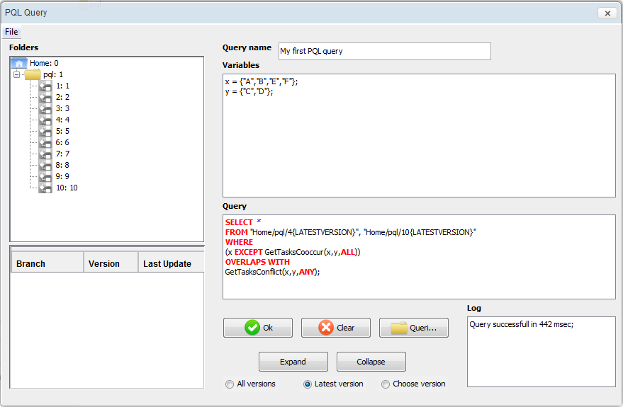
Figure 10. The PQL query editor in Apromore.

Process models in the Apromore repository get converted to Petri net systems and then indexed by the PQL bots. The interface of Apromore has been extended to allow users to specify PQL queries. The interface is designed to improve user experience, for example, by suggesting standard PQL keywords and allowing to drag-and-drop process models to be considered as part of the FROM clause. A PQL query entered using the Apromore interface is passed to the PQL tool. Based on the constructed indexes, the PQL tool evaluates the query. The result of the query, i.e., a set of the unique identifiers of models that match the query, is channeled back to Apromore. Apromore then displays to the user the list of models (and their attributes) that match the query. The user can examine the matching models using the Apromore’s model editor.

The reader can take a look at a screencast that demonstrates the use of PQL in Apromore, cf. https://www.youtube.com/watch?v=S_U6frTWd3M. Figure 10 shows a screenshot of the Apromore’s PQL query editor. The editor specifies a query similar to query Q10 from Section 4.7. In contrast to query Q10, the query in Figure 10 uses two variables ‘x’ and ‘y’, and requests to be executed over the latest versions of two models with names ‘4’ and ‘10’ located in folder ‘Home/pql/’.

Figure 11 shows another screenshot with information on the execution of yet another PQL query. Concretely, the information displayed is the explanation of the label similarities used to execute the query. As label “compensation plan is approved” is an instance of the ExactTask construct, according to the semantics of PQL, it resolves into the singleton that contains the label. Note that label “delegation of requirement for planning” is an instance of the DefSimTask construct. The PQL Tool used to execute this query was configured to use the default label similarity threshold of 0.75. Based on the configured engine for scoring label similarities, and the threshold, the PQL tool has discovered three similar labels shown in the figure.

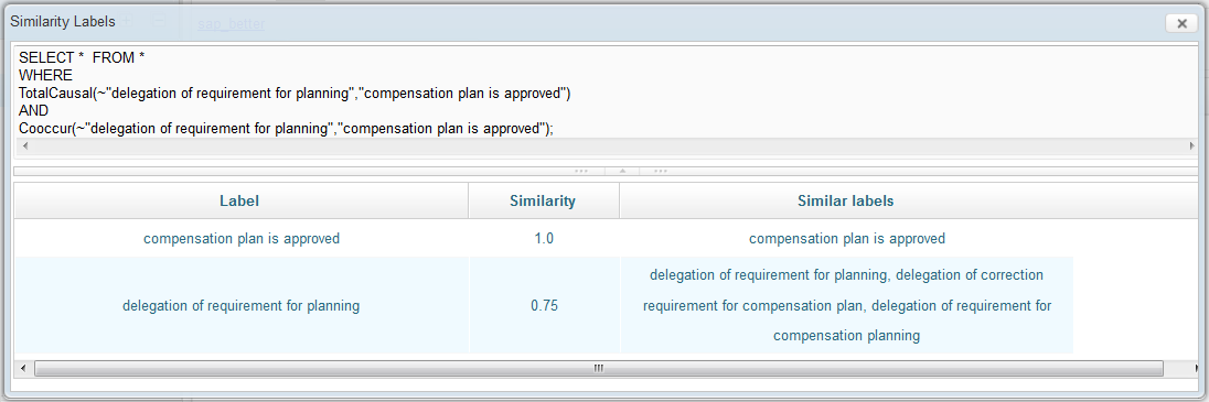
Figure 11. The PQL query info window, borrowed from (Polyvyanyy et al., 2015a).

6. Evaluation

Using the implementation from Section 5, we conducted a series of experiments to assess the performance of PQL in terms of indexing and querying time. The experiments were performed on a computer with 8GB of RAM and 3.4GHz quad-core Intel Core CPU (8 logical processors), running Windows 7 and JVM 1.7. The results demonstrate the feasibility and scalability of using PQL in industrial settings. Section 6.1 proceeds with a presentation of the datasets used in the evaluation.

6.1. Datasets

Process models. The study was conducted using 493 industrial and 1,000 synthetic process models. All the 1,493 models are sound workflow systems; the reader can refer to Section 3 for more information on sound workflow systems. We obtained the industrial models from the SAP R/3 Reference Model (Curran et al., 1998), which is a collection of 604 EPCs in various domains such as sales, production, and procurement used to customize the SAP R/3 ERP system. We converted the EPCs to Petri net systems and then completed them to workflow systems. Next, we filtered out the unsound systems, resulting in 493 sound models. We complemented this collection of real-life models with a collection of synthetic workflow systems, which we generated using the tool described in (Yan et al., 2015). This tool takes a seed process model collection and generates models that share similar structural and label characteristics to the seed. We used the 604 EPCs in the SAP R/3 collection as a seed, with a multiplier of 50, to generate 30,200 artificial EPCs. We converted these EPCs into workflow systems and filtered out the unsound models, leading to 16,769 sound workflow systems. Finally, from these 16,769 systems, we randomly selected 1,000 systems, each with more than 10 nodes.

Table 9. Structural characteristics of the industrial process models.

	#P	#T	#F	#OT	#XS	#XJ	#AS	#AJ	#PG	#B	#R
Average	17.85	15.91	35.7	8.57	0.64	0.65	1.13	1.13	5.73	1.78	0.002
Minimum	4	3	6	2	0	0	0	0	1	0	0
Maximum	74	86	180	35	6	6	6	6	31	9	1
Std. Dev.	12.73	11.89	27.61	6.21	0.89	0.91	1.21	1.22	4.93	1.66	0.05

Tables 9 and 10 provide statistics on the structural properties of the two model collections. The tables list basic statistics on the number of places (#P), transitions (#T), flow arcs (#F), observable transitions (#OT), XOR-splits (#XS), XOR-joins (#XJ), AND-splits (#AS), AND-joins (#AJ), polygons (#PG), bonds (#B), and rigids (#R) in the models of both collections, which are the metrics for comparing the structural properties of model collections employed in (Yan et al., 2015). By XOR-join and XOR-split we refer to a place with multiple input transitions and a place with multiple output transitions, respectively. By AND-join and AND-split we refer to a transition with multiple input places and a transition with multiple output places, respectively. Polygons, bonds and rigids are different types of SESE components in the WF-tree of a workflow system (Weidlich et al., 2011), where a polygon is a sequence of SESE components in which every two subsequent components share one node, a bond is a collection of SESE components that share entry and exit nodes, and a rigid is an unstructured component (Polyvyanyy, 2012). The tables demonstrate that industrial and synthetic models have similar structural characteristics.

Table 10. Structural characteristics of the synthetic process models.

	#P	#T	#F	#OT	#XS	#XJ	#AS	#AJ	#PG	#B	#R
Average	16.63	13.52	32.4	10.95	0.45	0.43	1.26	1.22	6.192	1.609	0.116
Minimum	5	5	10	3	0	0	0	0	1	0	0
Maximum	86	84	190	67	8	5	7	6	39	8	2
Std. Dev.	11.14	9.01	23.08	7.48	0.85	0.77	1.04	0.98	4.99	1.15	0.34

Queries. We designed 150 PQL query templates. Each template is a PQL query with placeholders for activity labels. During the experiments, the placeholders were instantiated with random labels. The query templates were developed to exploit the various features of the PQL grammar. According to the PQL features they support, these query templates were divided into three categories and further subdivided into groups and subgroups. Table 11 lists all the PQL query categories, groups, and subgroups, and provides numbers of query templates accordingly (see column “# Templates”). All the PQL query templates used in the experiments are listed in Appendix C.

Table 11. Categories, Groups, and Subgroups of PQL query templates.

Category.Group.Subgroup	Name	# Templates
1.a	Unary atomic predicates	2
1.b	Binary atomic predicates	4
2.a.1	Negations of predicates (Same)	6
2.a.2	Conjunctions of predicates (Same)	18
2.a.3	Disjunctions of predicates (Same)	18
2.b.1	Conjunctions of predicates (Mixed)	3
2.b.2	Disjunctions of predicates (Mixed)	3
2.b.3	Combinations of logical operations	2
3.a.1	Unary predicate macros	12
3.a.2	Binary predicate macros (Task-Set)	24
3.a.3	Binary predicate macros (Set-Set)	36
3.b.1	Constructions via unary predicates	2
3.b.2	Constructions via binary predicates	8
3.b.3	Constructions with set operations	5
3.b.4	Constructions with set comparisons	7

The first category contains six query templates capturing individual atomic behavioral predicates. These can be divided into two groups, one covering the two unary predicates (1.a), the other covering the four binary predicates (1.b).

The second category is a result of combining atomic predicates via logical operations. There are two groups, one for connecting the same predicates (2.a), the other for connecting mixed predicates (2.b). The former group can be further divided into three subgroups which capture, respectively, the negation of each predicate (2.a.1), the conjunctions of each predicate twice, three, or four times (2.a.2), and the disjunctions of each predicate twice, three, or four times (2.a.3). The latter group also has three subgroups which capture, respectively, the conjunctions of any two, three, or four different predicates (2.b.1), the disjunctions of any two, three, or four different predicates (2.b.2), and a couple of different combinations of three logical operations between mixed predicates (2.b.3).

The third category captures predicate macros in one group (3.a) and construction of task sets using predicates in the other group (3.b). The first group has three subgroups. One applies each of the unary predicate macros over a task set of two, three, or four tasks in conjunction (ALL) or in disjunction (ANY) (3.a.1); one applies each of the binary predicate macros between a single task and a task set of two, three, or four tasks in conjunction or in disjunction (3.a.2); and one applies each of the binary predicate macros between two task sets each consisting of two, three, or four tasks (3.a.3). The second group has four subgroups. The first two subgroups apply the set predicate TaskInSetOfTasks to a task set that is constructed using unary behavioral predicates (3.b.1) or using binary predicates (3.b.2). The last two subgroups capture task set constructions using mixed behavioral predicates with set operations (3.b.3) or set comparisons (3.b.4).

6.2. Indexing Performance

We conducted four experiments to measure the performance of PQL bots and the impact of different factors on indexing time. In what follows, for each of these four experiments, we detail its setup and discuss the obtained measurements.

Experiment 1.1: Impact of PQL bots on indexing time. The goal of this experiment was to measure the performance of PQL bots. We measured the time of indexing the industrial and synthetic models using different numbers of bots (from 1 to 8). Each indexing exercise was repeated three times and we recorded the average indexing times of the three runs. In all the runs, the bots were configured to only index the label similarity threshold of 1.0. The procedure was repeated for different parts of the process model collections, i.e., using 25%, 50%, 75% and 100% of models in each collection. Models for each part of each process model collection were selected randomly.

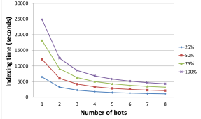
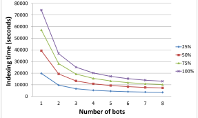
Figure 12. Impact of PQL bots on indexing time: (a) industrial models and (b) synthetic models.

Figure 12 plots the indexing times (in seconds) for different parts of process model collections against different numbers of PQL bots for (a) the industrial models and (b) the synthetic models. The two plots demonstrate that adding bots decreases indexing time, though the decrease in indexing time gets less pronounced with the increase of the number of bots. Indexing of the whole collection of industrial models with one bot took 6 hours and 54 minutes. Two bots managed to index 493 systems in 3 hours and 28 minutes (approximately two times faster than with one bot). Note that eight bots spent 1 hour and 12 minutes indexing the same collection (5.8 times faster than with one bot). A similar trend can be observed for the synthetic models. The relationship between the indexing time and the number of bots is best described by the power function $y=t\times x^{k}$, where $x$ is the number of bots and $y$ is the indexing time. For the industrial process models, the estimated values for constant $t$ are 6,065.6, 11,241, 16,735, and 23,071, for 25%, 50%, 75%, 100% of models in the collection, respectively. The estimated values for coefficient $k$ are -0.845, -0.834, -0.826, and -0.839, for 25%, 50%, 75%, 100% of models in the industrial collection, respectively. For the synthetic process models, the estimated values for constant $t$ are 17,991, 35,494, 52,086, and 68,077, for 25%, 50%, 75%, 100% of models in the collection, respectively. The estimated values for coefficient $k$ are -0.833, -0.806, -0.827, and -0.834, for 25%, 50%, 75%, 100% of models in the synthetic collection, respectively. The coefficient of determination $R^{2}$ ranges from 0.9901 to 0.9936 for the industrial process models and from 0.9834 to 0.9884 for the synthetic process models, indicating that the fitted functions can explain most of the variance in the indexing time.

This experiment also shows that the indexing time grows linearly with the size of a process model collection. Using one PQL bot, 25% of models in the industrial collection were indexed in 1 hour and 48 minutes, 50% were indexed in 3 hours and 22 minutes, 75% in 5 hours and 2 minutes, and the whole collection was indexed in 6 hours and 54 minutes. This relationship between the indexing time and the size of the collection is best captured by the linear function $y=49.549x+158.65$, where $x$ is the number of models in the collection and $y$ is the indexing time. The coefficient of determination $R^{2}$ for the above example is 0.9985. The coefficients of determination $R^{2}$ for the fitted linear functions on four data points range from 0.9985 to 0.9997 (for different numbers of bots). We observed the same trend for the synthetic collection, with $R^{2}$ values ranging from 0.9949 to 0.9992.

Experiment 1.2: Impact of model size on indexing time. The goal of this experiment was to assess the impact of size of a model on its indexing time. The two model collections were indexed three times (using one bot) and for each model we recorded the average indexing time of the three runs. The bot was configured to only index the label similarity threshold of 1.0.

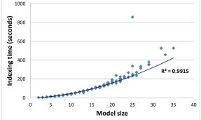
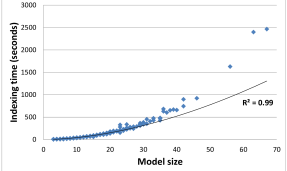
Figure 13. Impact of model size on indexing time: (a) industrial models and (b) synthetic models.

Figure 13 plots the indexing times (in seconds) against different sizes of workflow systems for (a) the industrial models and (b) the synthetic models. In this experiment, the size of a workflow system is measured as the number of its observable transitions; the reason for this is that bots index behavioral relations over observable transitions. The observed average indexing time of a model in the industrial collection is 50.3 seconds, with a minimum of 4.0 seconds (for a model with 2 observable transitions) and a maximum of 858.7 seconds (for a model with 25 observable transitions). We have also observed that 95% of models in the industrial collection can be indexed in less than 200 seconds. The average indexing time of a model in the synthetic collection is 74.0 seconds, with a minimum of 6.3 seconds (for a model with 3 observable transitions) and a maximum of 2,465.7 seconds (for a model with 67 observable transitions). The obtained measurements report that 95% of models in the synthetic collection can be indexed in less than 250 seconds.

The relation between the indexing time and the model size in the industrial collection is best approximated by the power function $y=0.8171\times x^{1.7579}$, which results in a coefficient of determination $R^{2}$ of 0.9915. One obvious outlier workflow system in the industrial collection (a model with 25 observable transitions whose indexing took 858.7 seconds) can be explained by the much bigger size of its state space (2,097,422 reachable states, measured by the LoLA tool) compared to the sizes of state spaces of the other models in the collection (equal or less than 262,156 reachable states). For the synthetic models, the relation between the indexing time and the model size is best explained by the power function $y=0.7423\times x^{1.7775}$, which results in $R^{2}$ = 0.99.

Given a system, either industrial or synthetic, we have noticed that it can be classified as an outlier using the value $f(x,y)=x^{2}\times\mathit{log}(y)$, where $x$ is the number of observable transitions of the system and $y$ is the size of the state space of the system in terms of the number of its reachable states. The Pearson’s correlation coefficient between the indexing times and the values of $f$ is $0.9426$ and $0.9692$ for the industrial and synthetic models, respectively. The residual analysis has revealed that the four outliers in the industrial collection are among the six models with the highest values of $f$, while the seven outliers in the synthetic collection are among the eight models with the highest values of $f$. The outliers were identified as models with the standardized residuals beyond $\pm 3$ units. The four outliers in the industrial collection have 25 (5 minutes and 38 seconds to index), 25 (14 minutes and 19 seconds), 32 (8 minutes and 48 seconds) and 35 (8 minutes and 48 seconds) observable transitions. Their state spaces comprise 114,717,  2,097,422,  390,  and 882 reachable states, respectively. The seven outliers in the synthetic collection have 36 (11 minutes and 23 seconds to index), 36 (10 minutes and 30 seconds), 42 (14 minutes and 58 seconds), 46 (15 minutes and 23 seconds), 56 (27 minutes and 10 seconds), 63 (39 minutes and 59 seconds), 67 (41 minutes and 6 seconds) observable transitions. Their state spaces have 303,118,  131,108,  103,694,  1,602,  5,730,  311,306,  and 6,818 reachable states, respectively.

Experiment 1.3: Impact of label similarity threshold on indexing time. The goal of this experiment was to assess the impact of different label similarity thresholds on the average time required to index a model. In this experiment, we varied the label similarity threshold (0.5, 0.6, 0.7, 0.8, 0.9 and 1.0) used to index the models. Both process model collections, i.e., the industrial and the synthetic, were indexed with one bot three times (for each similarity threshold), and average indexing times for the three runs were recorded. The Lucene-VSM label comparison method was used in all the runs, refer to Section 5 for details. The measured average indexing times of an industrial model for the label similarity thresholds 0.5, 0.6, 0.7, 0.8, 0.9, and 1.0 are 49.73, 50.3, 50.44, 50.48, 50.3, 50.31 seconds, respectively, with the standard deviation in the range from 80.28 to 81.35 seconds. The measured average indexing times of a synthetic model for the label similarity thresholds 0.5, 0.6, 0.7, 0.8, 0.9, and 1.0 are 74.53, 74.63, 74.62, 74.57, 74.61, 74.48 seconds, respectively, with the standard deviation in the range from 154.62 to 155.26 seconds.

There is no strong observed relation between the label similarity thresholds and the measured average indexing times, both for industrial and synthetic models. We conclude that the impact of different label similarity thresholds on indexing times is negligible. This can be explained by the small number of unique labels in both collections (2,278 unique labels across the industrial models and 10,473 unique labels across the synthetic models) and the fact that the labels are short character strings (on average 4.84 and 6.08 words in a label of an industrial and a synthetic model, respectively), whereas modern information retrieval engines are known to be efficient on collections that comprise millions of natural language documents of much larger sizes (Baeza-Yates and Ribeiro-Neto, 2011).

Experiment 1.4: Impact of index size on indexing time. The goal of this experiment was to measure the impact of index size on the average time required to index a model. To this end, we randomly split the industrial collection into four sets of (approximately) the same size (Sets 1–4). Each set was indexed four times: once when the index was empty, and then after 25%, 50% and 75% of the collection was indexed. In total, we performed four indexing runs. In the first run, Set 1 was indexed first, followed by indexing of Set 2, followed by Set 3, and finally concluded by indexing Set 4. The second run indexed the models in the order of Set 4, Set 1, Set 2, and finally Set 3. The third run indexed the models in the order of Set 3, Set 4, Set 1, and finally Set 2. The fourth run indexed the models in the order of Set 2, Set 3, Set 4, and finally Set 1. In all the runs, the same label similarity threshold of 1.0 was used. All the four indexing runs were accomplished by one PQL bot.

For all the sets, we observed that the average indexing time is not significantly affected by the size of the index. For models in Set 1, the recorded average indexing times are 53.63 seconds, 53.65 seconds, 54.09 seconds, and 54.26 seconds in the first, second, third, and the fourth run, respectively. For models in Set 2, the recorded average indexing times are 53.29 seconds, 53.46 seconds, 53.70 seconds, and 53.80 seconds in the first, second, third, and the fourth run, respectively. For models in Set 3, the recorded average indexing times are 44.75 seconds, 44.79 seconds, 44.93 seconds, and 45.15 seconds in the first, second, third, and the fourth run, respectively. Finally, for models in Set 4, the recorded average indexing times are 49.6 seconds, 49.52 seconds, 49.9 seconds, and 49.92 seconds in the first, second, third, and the fourth run, respectively. Given any set out of the four sets of models, the relation between the index size (used as a starting point to index the given set) and the average indexing time of a model in the set is best approximated by a polynomial function. The average indexing time for an industrial model in different sets at different positions in the indexing queue ranges from 44.75 to 54.26 seconds, with the difference between the maximum and minimum average indexing time for a given set at different indexing positions always being within 0.65 seconds. The measured coefficients of determination are equal to 0.9215, 0.9847, 0.9998, and 0.7366 for Set 1, Set 2, Set 3, and Set 4, respectively. The experiment demonstrates a general trend of a negligible increase in the indexing time with the growth of the index size. This observation can be explained by the fact that the introduced overhead is due to write operations on the PQL index, which can be efficiently handled by modern database management systems.

In the measurements of the average indexing times for the synthetic collection we observed a similar trend as in the measurements for the industrial collection. In particular, given any set out of the four sets of models in the synthetic collection (note that each set of synthetic models is composed of 250 random models), the relation between the index size (used as a starting point to index the given set) and the average indexing time of a model in the set is best approximated by a polynomial function. The average indexing time for a synthetic model in different sets at different positions in the indexing queue ranges from 61.7 to 86.74 seconds, with the difference between the maximum and minimum average indexing time for a given set at different indexing positions always being within 0.75 seconds. The measured coefficients of determination are equal to 0.8456, 0.9947, 0.9999, and 0.8545 for Set 1, Set 2, Set 3, and Set 4, respectively.

6.3. Querying Performance

We conducted three experiments to assess the performance of executing different types of PQL queries. The queries were generated from the templates discussed in Section 6.1. To conduct the evaluation, for each model collection and for each template we generated three queries by populating them with labels randomly selected from all the labels in the collection.

Experiment 2.1: Impact of query threads on querying time. This experiment measured the impact of the number of query threads and the size of a model collection on the querying time. We varied the number of query threads (from 1 to 8) and executed all the generated queries on different parts of the collections (25%, 50%, 75%, and 100% of models in each collection). For each part of each collection, models were randomly selected three times and the average querying times for the three runs were recorded. The models were indexed using the label similarity threshold of 1.0.

Figure 14 plots the querying times (in seconds) for different parts of process model collections against different numbers of query threads for (a) the industrial models and (b) the synthetic models. It demonstrates that additional query threads decrease querying time. As in Experiment 1.1, the gain in performance gets less pronounced with the increase of the number of query threads. For example, querying of the industrial models with one thread took on average 8.259 seconds, two threads managed to accomplish queries over 493 systems in 6.109 seconds (1.35 times faster than using one thread), while eight thread used 2.037 seconds to execute a query over the whole collection (four times faster than with one thread). A similar trend can be observed for the synthetic models.

The relation between the querying time and the number of threads is best captured by the power function $y=t\times x^{k}$, where $y$ is the querying time and $x$ is the number of query threads. For the industrial process models, the estimated values for constant $t$ are 2.0793, 4.1112, 6.3066, and 8.3917, for 25%, 50%, 75%, 100% of models in the collection, respectively. The estimated values for coefficient $k$ are -0.582, -0.584, -0.595, and -0.594, for 25%, 50%, 75%, 100% of models in the industrial collection, respectively. For the synthetic process models, the estimated values for constant $t$ are 4.1811, 8.6902, 13.693, and 19.444, for 25%, 50%, 75%, 100% of models in the collection, respectively. While the estimated values for coefficient $k$ are -0.581, -0.597, -0.604, and -0.612, for 25%, 50%, 75%, 100% of models in the synthetic collection, respectively. The coefficient of determination $R^{2}$ ranges from 0.9969 to 0.9982 for the industrial models and from 0.9983 to 0.9989 for the synthetic models, indicating that the fitted models can explain most of the variance in the querying time.

The measurements obtained in this experiment can be used to show that the querying time grows linearly with the size of a process model collection. For example, the measured average querying time with one query thread over 25% of the industrial models is 2.037 seconds, over 50% is 4.037 seconds, over 75% is 6.109 seconds, and over the whole collection is 8.259 seconds. This trend is best described by the linear relation $y=0.0168\times x-0.0658$, where $x$ is the number of models in the collection and $y$ is the querying time. The coefficient of determination $R^{2}$ for the above example is 0.9998. The coefficients of determination $R^{2}$ for the fitted linear functions on four data points range from 0.9988 to 1.0 (for different numbers of query threads). We observed the same trend for the synthetic collection, with $R^{2}$ values ranging from 0.9967 to 0.9998.

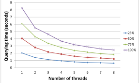
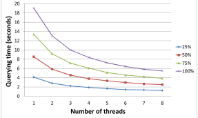
Figure 14. Impact of query threads on querying time: (a) industrial models and (b) synthetic models.

Experiment 2.2: Impact of query types on querying time.

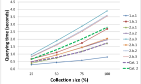
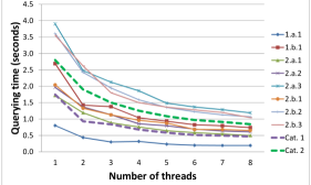
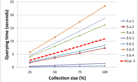
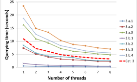
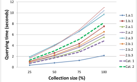
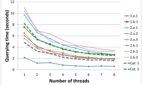
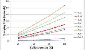
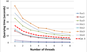
Figure 15. The average querying times for different model collection sizes (a,c,e,g) and for different numbers of query threads (b,d,f,h); PQL queries in Cats. 1 and 2 for the industrial models (a,b) and for the synthetic models (e,f), and PQL queries in Cat. 3 for the industrial models (c,d) and for the synthetic models (g,h).

This experiment aimed to assess the impact of different query types on querying time. It uses the same setup as Experiment 2.1. In this experiment, we measured querying times for different query groups discussed in Section 6.1.

Figs. 15 and 15 show the average querying times for the collection of industrial models for queries in Categories 1 and 2, while Figs. 15 and 15 show the average querying times for queries in Category 3. The average querying times for the synthetic collection are shown in Figs. 15 and 15 (Categories 1 and 2) and Figs. 15 and 15 (Category 3). Queries in Category 1 only comprise atomic predicates and, thus, are the fastest. The measured average querying time for the Category 1 queries using one query thread is 1.75 seconds for the 493 models in the industrial collection (approximately 3.5ms per one model-query check) and 4.84 seconds for the 1,000 models in the synthetic collection (approximately 4.8ms per one model-query check). With eight query threads, the Category 1 queries were on average accomplished in 0.47 seconds for the 493 models in the industrial collection and 1.61 seconds for the 1,000 models in the synthetic collection. Queries in Category 2 comprise atomic predicates and logical connectives. Thus, they require a bit more time to accomplish than queries in Category 1. The measured average querying time for Category 2 queries with one thread is 2.8 seconds for the industrial models and 8.2 seconds for the synthetic models. With eight query threads, it is 0.84 and 2.52 seconds for the industrial and synthetic models, respectively. Queries in Category 3 comprise macros and, hence, are the lengthiest. The measured average querying time for Category 3 queries with one query thread is 10.89 seconds for the industrial models (approximately 11ms per one model-query check) and 24.76 seconds for the synthetic models (approximately 25ms per one model-query check). With eight query threads, it is 3.23 and 6.96 seconds for the industrial and synthetic models, respectively.

Figs. 15, 15, 15 and 15 demonstrate the linear dependency between the number of models in a collection and querying time for different query types. The coefficients of determination $R^{2}$ for the fitted linear functions for different query subgroups range from 0.9718 to 1.0 for the industrial models and from 0.9592 to 0.9992 for the synthetic models. Finally, Figs. 15, 15, 15, and 15 show that for all the query subgroups the relation between the querying time and the number of query threads follows the trend observed in Experiment 2.1. The coefficients of determination $R^{2}$ for the fitted power functions for different query subgroups range from 0.9724 to 0.998 for the industrial models and from 0.9329 to 0.9955 for the synthetic models.

Experiment 2.3: Impact of label similarity on querying time. The aim of this experiment was to measure the impact of label similarity on querying time. To this end, we repeated Experiment 2.1 with the following modifications: (i) the bots were configured to index label similarity thresholds of 0.75 and 1.0, (ii) all the query templates were augmented to include the “tilde” symbol immediately before every activity label (thus, similar labels were considered during querying), and (iii) the tool was configured to use a default label similarity threshold of 0.75.

We compared the measured querying times with the querying times obtained in Experiment 2.1. For the industrial process models, the querying times (using one query thread) on average are 10.9% higher for queries that account for similar labels. For the synthetic process models, the querying times (again, using one query thread) on average are 9.47% higher for queries that account for similar labels. This small overhead can be explained by the fact that the PQL tool indexes behavioral relations at the level of PQL tasks and, thus, at runtime, the overhead is only due to the additional time required to retrieve information on the indexed PQL tasks.

7. Related Work

Recently, we conducted a systematic literature review of the state of the art methods for querying process repositories (Polyvyanyy et al., 2017). As part of that study, we designed a framework for developing process querying methods. The framework is an abstract system in which components can be selectively replaced to result in a new process querying method. According to this framework, PQL addresses querying of formal process models using a query language with a formal semantics that implements the read querying intent, i.e., is designed to retrieve models from repositories. Two recent surveys of process querying methods (Wang et al., 2014; Polyvyanyy et al., 2017) confirm that query languages with these characteristics constitute a gap in the area of process querying. In (Polyvyanyy, 2018), we categorized and summarized the existing process querying methods. According to that classification, two prominent existing works for behavioral querying of process models that share similar characteristics with PQL are the works on “Behavior Query Language” (BQL) (Jin et al., 2011) and “A Process-model Query Language” (APQL) (ter Hofstede et al., 2013). Next, we briefly review APQL and BQL, summarize some important results on behavioral predicates, and discuss several related techniques from the areas outside process querying.

Behavioral querying. PQL is inspired by our work on APQL and redesigns APQL in many respects. PQL differs from APQL in that it is grounded in a different and empirically justified collection of behavioral predicates, extends the abstract syntax of APQL, proposes a concrete syntax, has an implementation that demonstrates its feasibility, and operates on the level of observable behaviors, i.e., incorporates mechanisms for interpreting two different tasks as such that have the same meaning for the purpose of evaluating the queries. If compared with BQL, PQL is rigorous since both the syntax and semantics of the language are formally defined. BQL is grounded in three behavioral predicates. All these predicates belong to the 4C spectrum and were included in our empirical study. These three predicates are Conflict (called “exclude” in (Jin et al., 2011)), ExistCausal (“precede”), and ExistConcurrent (“parallel with”), refer to Section 4.1.1 for more details. As a result of our empirical evaluation, only one of these three predicates, namely Conflict, was selected to be included in the set of eight core PQL predicates. As to ExistCausal and ExistConcurrent, the stakeholders have given their preference to “stronger” predicates of TotalCausal and TotalConcurrent, which ensure that the respective behavioral relation holds for all (rather than only for some) occurrences of the tasks. Finally, the fundamental difference between PQL and BQL is that BQL predicates are defined over occurrences of tasks, while PQL predicates are defined over aggregations (derived using quantification) over the occurrences of tasks.

Model Checking. Model checking studies problems that can verify various properties of process models (Chan et al., 1998; Baier and Katoen, 2008). A model checking problem is a problem that, given a formal specification of a property, usually captured using some specification language, and a process model, answers whether the property holds in the given model. Often, in order to solve the problem, a model checking technique proceeds by constructing an alternative representation of the model that indicates whether the given property holds or not in the model. Model checking techniques usually use temporal logics as property specification languages, e.g., linear temporal logic (LTL) and computational tree logic (CTL). Model checking techniques can be employed for process querying to retrieve process models that fulfill a given property (Gurfinkel et al., 2003).

As recently demonstrated by Wolf (Wolf, 2018), computations of most of the 4C behavioral relations can be reduced, via non-trivial transformations that require exponential space, to classical interleaving-based model checking problems. Only one problem remains completely unsolved, whereas several problems were solved in the absence of auto-concurrency. In fact, based on the results reported in (Polyvyanyy et al., 2014b; Wolf, 2018), we know that all the predicates selected for inclusion into PQL, refer to Section 4.1.3, can be reduced to model checking problems. However, one cannot directly apply the proposed solutions for process querying. Note that the proposed in (Wolf, 2018) LTL and CTL properties for computing the 4C relations are formulated over the transformed models and, hence, do not convey the meanings of the properties to be computed, which makes them unsuitable for the user interpretations. Also, the performance of the approach proposed in (Wolf, 2018) has not been evaluated; note that model checking on infinite-state systems is undecidable and is PSPACE-complete on finite state systems (Esparza and Nielsen, 1994). Such an evaluation, and development of new efficient techniques for computing the 4C relations, may contribute to the development of PQL.

Behavioral predicates. In (Dwyer et al., 1999), the authors report the results of a survey of property specifications (a.k.a. behavioral predicates) captured in temporal logics, e.g., LTL or CTL. The authors collected and classified 555 properties, most of which are specified in LTL, from a wide range of domains, including hardware protocols, communication protocols, avionics, operating systems, and database systems. Interestingly, the authors conclude that “even with significant expertise, dealing with the complexity of such a specification [a temporal logic property] can be daunting” and suggest that often “complexity is addressed by the definition and use of abstraction”. PQL implements such an abstraction. There are no translations from PQL predicates to temporal logic properties over concepts of the original process model, see above. However, it is easy to see that several properties surveyed in (Dwyer et al., 1999) can be expressed as logical expressions over the 4C spectrum relations. A comprehensive study of such translations is an interesting direction to explore.

To the best of our knowledge, there are no existing works that study the relevance of behavioral predicates for the purpose of querying (business) process models. Future empirical studies will aim at gaining a better understanding of the suitability of behavioral predicates for process querying, as per the process querying compromise between decidable, efficiently computable, and suitable process querying methods (Polyvyanyy et al., 2017).

Verification of software systems. In (Dwyer et al., 2004), the authors proposed FLAVERS—a finite-state verification technique to analyze whether a concurrent software system satisfies a given user-specified property. To perform the verification, FLAVERS constructs an abstract representation of the system. This abstraction step comes at a price of precision of the analysis results. In our work, we suggest using PQL to query repositories of business process models. However, one can explore PQL for querying, testing, and verification of software systems. Unlike FLAVERS, PQL is precise, i.e., the result of every PQL query is free from false positive and false negative errors. FLAVERS and PQL differ in how they interpret models of analyzed models, according to the interleaving and noninterleaving semantics of concurrent systems (Sassone et al., 1996), respectively. Thus, PQL can be used to express properties that address potential simultaneous execution of instructions of software systems.

In software engineering, well-established finite-state verification techniques, like the methods based on classical model checking or the FLAVERS technique, are used to inform continuous improvement of processes (Clarke et al., 2008; Osterweil et al., 2017). PQL can enrich this repertoire of verification techniques for detecting errors in semantically rich process models with user interpretable and relevant properties.

Declarative process discovery. Process mining assists business analysts in dealing with the emerging complexities and uncertainties introduced by business processes, as it aims to discover, monitor and improve processes observed in the real world using the knowledge accumulated in event logs produced by modern information systems (van der Aalst, 2016). An event log is a collection of traces, each representing events executed by a business process. The process discovery problem consists of obtaining a good process model that describes the behavior recorded in a given event log. Declarative process discovery aims to construct such process models as collections of declarative constraints over possible executions of business activities. These declarative constraints are often expressed as behavioral predicates, similar to those used in PQL.

In (Ciccio and Mecella, 2015), the authors proposed an algorithm for declarative process discovery, called MINERful. The algorithm performs the statistical analysis of the input event log, and then uses the derived knowledge to compose the declarative constraints which collectively describe the traces recorded in the event log. In particular, MINERful discovers Declare constraints (van der Aalst et al., 2009), which is a particular repertoire of 20 LTL templates. In (Westergaard et al., 2013), the authors propose another algorithm capable of discovering Declare constraints from event logs, called UnconstrainedMiner. To address the problem of LTL semantics over finite traces, in that work, Declare templates are translated to regular expressions.

Next generation declarative process discovery algorithms can target discovery of the 4C spectrum constraints, in general, and PQL predicates, in particular. This will allow overcoming two limitations of the existing techniques: the inability of encoding noninterleaving semantics (Sassone et al., 1996) and lack of empirical justification of the discovered constraints.

8. Conclusion

This paper proposed a query language for retrieving models from process model repositories. The language has an SQL-like syntax to facilitate ease of use and its basic predicates are empirically grounded. Noteworthy is also the fact that the language targets process behavior rather than structural aspects of process models. This focus on the behavior seems more natural than the usual way of querying the representations of the behavior. The language supports label similarity, i.e., labels are assessed as to whether they are sufficiently similar (which is determined with respect to a given threshold) to another label. Support for this feature is essential as variations on task names can easily emerge when a range of people are involved in the creation of process models.

The proposed query language has been implemented and its runtime performance evaluated using real-life and synthetic process models. The conducted experiments indicate the feasibility of computing the basic PQL predicates and demonstrate that the implemented PQL Tools can execute PQL queries in almost real-time.

There are several limitations of this work that should be acknowledged. Some of these limitations naturally give rise to possible avenues for future work.

First of all, the expressiveness of the proposed query language is constrained by the choice of basic predicates. As it turns out though, this is a fundamental limitation that no semantic process model query language grounded in behavioral predicates can escape (Polyvyanyy et al., 2016). Expressiveness can be extended, for instance, by allowing the use of example executions in queries, in particular executions that contain wildcards to express search intents like “find all process models that allow the execution $\left\langle\texttt{a},\texttt{b},*,\texttt{b},\texttt{b},*,\texttt{c},*\right\rangle$”. Through the use of wildcards one can search for those process models in which any trace that fits the template can be executed.

Second, the proposed design of PQL, and the design of its subsequent versions, should be justified by new empirical evidence. For example, it is important to study the ratio between the queries that users want to express and PQL can support and to improve the language accordingly. One can conduct empirical studies to assess how simple it is for the users to specify complex behavioral queries, and use the obtained insights to simplify the language. As another example, one can empirically assess the usefulness of the proposed exploratory search principle.

Third, the proposed query language is only concerned with control-flow aspects of process models and does not take the data and resource perspectives into account. The potential use of the query language can be widened by allowing queries that refer to aspects other than control-flow.

Fourth, PQL can be extended with functionality that is auxiliary to behavioral querying, e.g., aggregate functions over retrieved processes. PQL predicates operate over the global process scope, i.e., over processes that represent completed executions of process models. Similar to some properties surveyed by Dwyer et al. (Dwyer et al., 1999), PQL predicates can be generalized to operate over other scopes, e.g., between given process conditions. However, it is worth mentioning that 80% of the surveyed in (Dwyer et al., 1999) properties address the global scope.

Fifth, PQL can be extended with manipulation statements (think INSERT, DELETE, UPDATE). Through the use of these statements, it should be possible to add, delete, and modify process models.

Another limitation concerns the requirement that the class of process models that the query language can deal with is the class of sound workflow systems. In practice, process models may not always be sound, for example as models may not yet have been completed, and it is worthwhile to explore how the current work could be adapted to allow for a wider class of process models.

Despite the benefits of a query language based on the behavior described in models, there is a drawback that the behavioral aspects can be complex and consequently query results may not always be intuitive to stakeholders. To facilitate query understanding, process models can be annotated to explain the reasons for their inclusion in the query results.

Acknowledgements

We would like to thank Jan Recker for his input in the design of the experiment on assessing practical relevance of using behavioral predicates for querying process repositories.

Appendix A Interview Instrument

This appendix contains the instrument used to conduct the empirical study reported in Section 4.1.

Appendix B PQL Grammar

This appendix specifies the complete grammar of the PQL language captured in the ANTLR notation. ANTLR (ANother Tool for Language Recognition) is a parser generator for reading and translating structured text or binary files (Parr and Quong, 1995; Parr, 2013). ANTLR can take a grammar of a language as input and generate source code for a parser that can build and walk syntax trees (Meyer, 1990). The language must be specified using a context-free grammar which is expressed using extended Backus-Naur Form (Hopcroft et al., 2006).

.7em

   // PQL version 1.0 grammar for ANTLR v4
   // [The "BSD licence"]
   // Copyright (c) 2014-2016 Artem Polyvyanyy
   // All rights reserved.

   grammar PQL;

   query      : variables
              SELECT attributes
              FROM locations
              (WHERE predicate)? EOS ;

   variables  : variable* ;
   variable   : varName ASSIGN
                setOfTasks EOS ;

   varName    : VARIABLE_NAME ;

   attributes : attribute (SEP attribute)* ;
   attribute  : universe
              | attributeName ;

   locations  : location (SEP location)* ;
   location   : universe
              | locationPath ;

   universe           : UNIVERSE ;
   attributeName      : STRING ;
   locationPath       : STRING ;

   setOfTasks : tasks
              | union
              | intersection
              | difference ;

   tasks      : varName
              | setOfAllTasks
              | setOfTasksLiteral
              | setOfTasksConstruction
              | setOfTasksParentheses ;

   setOfAllTasks      :
              GET_TASKS LP RP;

   setOfTasksLiteral  :
              LB (task (SEP task)*)? RB ;

   task       : approximate label
              | label (LSB similarity RSB)? ;

   approximate: TILDE ;
   label      : STRING ;
   similarity : SIMILARITY ;

   setOfTasksConstruction      :
                unaryPredicateConstruction
              | binaryPredicateConstruction ;

   unaryPredicateConstruction  :
                (GET_TASKS)unaryPredicateName
                LP setOfTasks RP ;

   binaryPredicateConstruction :
                (GET_TASKS)binaryPredicateName
                LP setOfTasks SEP setOfTasks
                SEP anyAll RP ;

   anyAll     : ANY | ALL ;

   unaryPredicateName : CAN_OCCUR
              | ALWAYS_OCCURS;

   binaryPredicateName: CAN_CONFLICT
              | CAN_COOCCUR
              | CONFLICT
              | COOCCUR
              | TOTAL_CAUSAL
              | TOTAL_CONCUR ;

   predicate  : proposition
              | conjunction
              | disjunction
              | logicalTest ;

   proposition: unaryPredicate
              | binaryPredicate
              | unaryPredicateMacro
              | binaryPredicateMacro
              | setPredicate
              | truthValue
              | parentheses
              | negation ;

   unaryPredicate      : unaryPredicateName
                LP task RP ;

   binaryPredicate     : binaryPredicateName
                LP task SEP task RP ;  ΨΨΨ

   unaryPredicateMacro : unaryPredicateName
                LP setOfTasks SEP anyAll RP ;
ΨΨ
   binaryPredicateMacro:
                binaryPredicateMacroTaskSet
              | binaryPredicateMacroSetSet ;

   binaryPredicateMacroTaskSet :
                binaryPredicateName LP task
                SEP setOfTasks SEP anyAll RP ;
ΨΨ
   binaryPredicateMacroSetSet  :
              binaryPredicateName
              LP setOfTasks SEP setOfTasks
              SEP anyEachAll RP ;

   anySomeEachAll  : ANY | SOME | EACH | ALL ;

   setPredicate: taskInSetOfTasks
              | setComparison ;

   taskInSetOfTasks : task IN setOfTasks ;

   setComparison    : setOfTasks
              setComparisonOperator
              setOfTasks ;

   setComparisonOperator : identical
              | different
              | overlapsWith
              | subsetOf
              | properSubsetOf ;

   truthValue : TRUE
              | FALSE ;

   logicalTest: isTrue
              | isNotTrue
              | isFalse
              | isNotFalse ;

   union      : (tasks | difference |
                intersection) UNION (tasks |
                difference | intersection)
                (UNION (tasks | difference
                | intersection))* ;

   intersection : (tasks | difference)
                  INTERSECTION
                  (tasks | difference)
                  (INTERSECTION (tasks
                  | difference))* ;

   difference   : tasks DIFFERENCE tasks
                | tasks DIFFERENCE
                  difference ;

   negation     : NOT proposition ;

   isTrue       : proposition IS TRUE ;
   isNotTrue    : proposition IS NOT TRUE ;
   isFalse      : proposition IS FALSE ;
   isNotFalse   : proposition IS NOT FALSE ;

   disjunction  : (proposition | logicalTest |
            conjunction) OR (proposition |
            logicalTest | conjunction) (OR
            (proposition | logicalTest
            | conjunction))* ;
ΨΨ
   conjunction  : (proposition | logicalTest)
            AND (proposition | logicalTest)
            (AND (proposition
            | logicalTest))* ;

   parentheses  : LP proposition RP
           | LP conjunction RP
           | LP disjunction RP
           | LP logicalTest RP ;

   setOfTasksParentheses : LP varName RP
           | LP universe RP
           | LP setOfTasksLiteral RP
           | LP setOfTasksConstruction RP
           | LP union RP
           | LP difference RP
           | LP intersection RP
           | LP setOfTasksParentheses RP ;

   UNIVERSE     : ’*’ ;

   STRING       : DQ ( ESC_SEQ
                | ~(’\\’|’"’) )* DQ ;
   VARIABLE_NAME: (’a’..’z’|’_’)
                  (’a’..’z’|’0’..’9’|’_’)*;
   SIMILARITY   : ’1’ | ’0’ (’.’ ’0’..’9’+)?
                | ’.’ ’0’..’9’+ ;

   LP          : ’(’ ;
   RP          : ’)’ ;
   LB          : ’{’ ;
   RB          : ’}’ ;
   LSB         : ’[’ ;
   RSB         : ’]’ ;
   DQ          : ’"’ ;
   EOS         : ’;’ ;
   SEP         : ’,’ ;
   ASSIGN      : ’=’ ;
   TILDE       : ’~’ ;

   ESC_SEQ     : ’\\’ (’\"’|’\\’|’/’|’b’|
               ’f’|’n’|’r’|’t’)
               | UNICODE_ESC ;
   UNICODE_ESC : ’\\’ ’u’ HEX_DIGIT
               HEX_DIGIT HEX_DIGIT HEX_DIGIT ;
   HEX_DIGIT   : (’0’..’9’|
               ’a’..’f’|’A’..’F’) ;
   WS          : [ \r\t\n]+ -> skip ;
   LINE_COMMENT: ’--’ ~[\r\n]* -> skip ;

   SELECT      : ’SELECT’ ;
   FROM        : ’FROM’ ;
   WHERE       : ’WHERE’ ;

   EQUALS      : ’EQUALS’ ;
   OVERLAPS    : ’OVERLAPS’ ;
   WITH        : ’WITH’ ;
   SUBSET      : ’SUBSET’ ;
   PROPER      : ’PROPER’ ;
   GET_TASKS   : ’GetTasks’ ;

   NOT         : ’NOT’ ;
   AND         : ’AND’ ;
   OR          : ’OR’ ;

   ANY         : ’ANY’ ;
   SOME        : ’SOME’ ;
   EACH        : ’EACH’ ;
   ALL         : ’ALL’ ;

   IN          : ’IN’ ;
   IS          : ’IS’ ;
   OF          : ’OF’ ;

   TRUE        : ’TRUE’ ;
   FALSE       : ’FALSE’ ;

   identical       : EQUALS ;
   different       : NOT EQUALS ;
   overlapsWith    : OVERLAPS WITH ;
   subsetOf        : IS SUBSET OF ;
   properSubsetOf  : IS PROPER SUBSET OF ;

   UNION           : ’UNION’ ;
   INTERSECTION    : ’INTERSECT’ ;
   DIFFERENCE      : ’EXCEPT’ ;

   CAN_OCCUR       : ’CanOccur’ ;
   ALWAYS_OCCURS   : ’AlwaysOccurs’ ;
   CAN_CONFLICT    : ’CanConflict’ ;
   CAN_COOCCUR     : ’CanCooccur’ ;
   CONFLICT        : ’Conflict’ ;
   COOCCUR         : ’Cooccur’ ;
   TOTAL_CAUSAL    : ’TotalCausal’ ;
   TOTAL_CONCUR    : ’TotalConcurrent’ ;

Appendix C PQL Queries

This appendix contains 150 PQL query templates used in the evaluation reported in Section 6. Each template is a PQL query with placeholders for activity labels. The templates can be instantiated with specific labels and used as a benchmark to evaluate performance of PQL tools. The query templates were developed to exploit the various features of the PQL grammar. According to the PQL features they support, these query templates are divided into three categories and further subdivided into groups and subgroups, refer to Section 6.1 for details.

Table 12. PQL query templates.

No.	ID	PQL template
1	1.a.1	SELECT * FROM * WHERE CanOccur("L1");
2	1.a.2	SELECT * FROM * WHERE AlwaysOccurs("L1");
3	1.b.1	SELECT * FROM * WHERE Cooccur("L1","L2");
4	1.b.2	SELECT * FROM * WHERE Conflict("L1","L2");
5	1.b.3	SELECT * FROM * WHERE TotalCausal("L1","L2");
6	1.b.4	SELECT * FROM * WHERE TotalConcurrent("L1","L2");
7	2.a.1.1	SELECT * FROM * WHERE NOT CanOccur("L1");
8	2.a.1.2	SELECT * FROM * WHERE NOT AlwaysOccurs("L1");
9	2.a.1.3	SELECT * FROM * WHERE NOT Cooccur("L1","L2");
10	2.a.1.4	SELECT * FROM * WHERE NOT Conflict("L1","L2");
11	2.a.1.5	SELECT * FROM * WHERE NOT TotalCausal("L1","L2");
12	2.a.1.6	SELECT * FROM * WHERE NOT TotalConcurrent("L1","L2");
13	2.a.2.1	SELECT * FROM * WHERE CanOccur("L1") AND CanOccur("L2");
14	2.a.2.2	SELECT * FROM * WHERE CanOccur("L1") AND CanOccur("L2") AND CanOccur("L3");
15	2.a.2.3	SELECT * FROM * WHERE CanOccur("L1") AND CanOccur("L2") AND CanOccur("L3") AND CanOccur("L4");
16	2.a.2.4	SELECT * FROM * WHERE AlwaysOccurs("L1") AND AlwaysOccurs("L2");
17	2.a.2.5	SELECT * FROM * WHERE AlwaysOccurs("L1") AND AlwaysOccurs("L2") AND AlwaysOccurs("L3");
18	2.a.2.6	SELECT * FROM * WHERE AlwaysOccurs("L1") AND AlwaysOccurs("L2") AND AlwaysOccurs("L3") AND AlwaysOccurs("L4");
19	2.a.2.7	SELECT * FROM * WHERE Cooccur("L1","L2") AND Cooccur("L3","L4");
20	2.a.2.8	SELECT * FROM * WHERE Cooccur("L1","L2") AND Cooccur("L3","L4") AND Cooccur("L5","L6");
21	2.a.2.9	SELECT * FROM * WHERE Cooccur("L1","L2") AND Cooccur("L3","L4") AND Cooccur("L5","L6") AND Cooccur("L7","L8");
22	2.a.2.10	SELECT * FROM * WHERE Conflict("L1","L2") AND Conflict("L3","L4");
23	2.a.2.11	SELECT * FROM * WHERE Conflict("L1","L2") AND Conflict("L3","L4") AND Conflict("L5","L6");
24	2.a.2.12	SELECT * FROM * WHERE Conflict("L1","L2") AND Conflict("L3","L4") AND Conflict("L5","L6") AND Conflict("L7","L8");
25	2.a.2.13	SELECT * FROM * WHERE TotalCausal("L1","L2") AND TotalCausal("L3","L4");
26	2.a.2.14	SELECT * FROM * WHERE TotalCausal("L1","L2") AND TotalCausal("L3","L4") AND TotalCausal("L5","L6");
27	2.a.2.15	SELECT * FROM * WHERE TotalCausal("L1","L2") AND TotalCausal("L3","L4") AND TotalCausal("L5","L6") AND TotalCausal("L7","L8");
28	2.a.2.16	SELECT * FROM * WHERE TotalConcurrent("L1","L2") AND TotalConcurrent("L3","L4");
29	2.a.2.17	SELECT * FROM * WHERE TotalConcurrent("L1","L2") AND TotalConcurrent("L3","L4") AND TotalConcurrent("L5","L6");
30	2.a.2.18	SELECT * FROM * WHERE TotalConcurrent("L1","L2") AND TotalConcurrent("L3","L4") AND TotalConcurrent("L5","L6") AND TotalConcurrent("L7","L8");
31	2.a.3.1	SELECT * FROM * WHERE CanOccur("L1") OR CanOccur("L2");
32	2.a.3.2	SELECT * FROM * WHERE CanOccur("L1") OR CanOccur("L2") OR CanOccur("L3");
33	2.a.3.3	SELECT * FROM * WHERE CanOccur("L1") OR CanOccur("L2") OR CanOccur("L3") OR CanOccur("L4");
34	2.a.3.4	SELECT * FROM * WHERE AlwaysOccurs("L1") OR AlwaysOccurs("L2");
35	2.a.3.5	SELECT * FROM * WHERE AlwaysOccurs("L1") OR AlwaysOccurs("L2") OR AlwaysOccurs("L3");
36	2.a.3.6	SELECT * FROM * WHERE AlwaysOccurs("L1") OR AlwaysOccurs("L2") OR AlwaysOccurs("L3") OR AlwaysOccurs("L4");
37	2.a.3.7	SELECT * FROM * WHERE Cooccur("L1","L2") OR Cooccur("L3","L4");
38	2.a.3.8	SELECT * FROM * WHERE Cooccur("L1","L2") OR Cooccur("L3","L4") OR Cooccur("L5","L6");
39	2.a.3.9	SELECT * FROM * WHERE Cooccur("L1","L2") OR Cooccur("L3","L4") OR Cooccur("L5","L6") OR Cooccur("L7","L8");
40	2.a.3.10	SELECT * FROM * WHERE Conflict("L1","L2") OR Conflict("L3","L4");
41	2.a.3.11	SELECT * FROM * WHERE Conflict("L1","L2") OR Conflict("L3","L4") OR Conflict("L5","L6");
42	2.a.3.12	SELECT * FROM * WHERE Conflict("L1","L2") OR Conflict("L3","L4") OR Conflict("L5","L6") OR Conflict("L7","L8");
43	2.a.3.13	SELECT * FROM * WHERE TotalCausal("L1","L2") OR TotalCausal("L3","L4");
44	2.a.3.14	SELECT * FROM * WHERE TotalCausal("L1","L2") OR TotalCausal("L3","L4") OR TotalCausal("L5","L6");
45	2.a.3.15	SELECT * FROM * WHERE TotalCausal("L1","L2") OR TotalCausal("L3","L4") OR TotalCausal("L5","L6") OR TotalCausal("L7","L8");
46	2.a.3.16	SELECT * FROM * WHERE TotalConcurrent("L1","L2") OR TotalConcurrent("L3","L4");
47	2.a.3.17	SELECT * FROM * WHERE TotalConcurrent("L1","L2") OR TotalConcurrent("L3","L4") OR TotalConcurrent("L5","L6");
48	2.a.3.18	SELECT * FROM * WHERE TotalConcurrent("L1","L2") OR TotalConcurrent("L3","L4") OR TotalConcurrent("L5","L6") OR TotalConcurrent("L7","L8");
49	2.b.1.1	SELECT * FROM * WHERE CanOccur("L1") AND Conflict("L2","L3");
50	2.b.1.2	SELECT * FROM * WHERE AlwaysOccurs("L1") AND Cooccur("L2","L3") AND TotalConcurrent("L4","L5");
51	2.b.1.3	SELECT * FROM * WHERE Cooccur("L1","L2") AND TotalCausal("L3","L4") AND TotalConcurrent("L5","L6");
52	2.b.2.1	SELECT * FROM * WHERE AlwaysOccurs("L1") OR Cooccur("L2","L3");
53	2.b.2.2	SELECT * FROM * WHERE CanOccur("L1") OR AlwaysOccurs("L2") OR Conflict("L3","L4");
54	2.b.2.3	SELECT * FROM * WHERE Conflict("L1","L2") OR TotalCausal("L3","L4") OR TotalConcurrent("L5","L6");
55	2.b.3.1	SELECT * FROM * WHERE AlwaysOccurs("L1") OR (Cooccur("L2","L3") AND (NOT TotalCausal("L4","L5")));
56	2.b.3.2	SELECT * FROM * WHERE (CanOccur("L1") AND (NOT Conflict("L2","L3"))) OR (TotalConcurrent("L4","L5") AND AlwaysOccurs("L6"));
57	3.a.1.1	SELECT * FROM * WHERE CanOccur([2ex].{"L1","L2"[2ex].},ALL);
58	3.a.1.2	SELECT * FROM * WHERE CanOccur([2ex].{"L1","L2","L3"[2ex].},ALL);
59	3.a.1.3	SELECT * FROM * WHERE CanOccur([2ex].{"L1","L2","L3","L4"[2ex].},ALL);
60	3.a.1.4	SELECT * FROM * WHERE CanOccur([2ex].{"L1","L2"[2ex].},ANY);
61	3.a.1.5	SELECT * FROM * WHERE CanOccur([2ex].{"L1","L2","L3"[2ex].},ANY);
62	3.a.1.6	SELECT * FROM * WHERE CanOccur([2ex].{"L1","L2","L3","L4"[2ex].},ANY);
63	3.a.1.7	SELECT * FROM * WHERE AlwaysOccurs([2ex].{"L1","L2"[2ex].},ALL);
64	3.a.1.8	SELECT * FROM * WHERE AlwaysOccurs([2ex].{"L1","L2","L3"[2ex].},ALL);
65	3.a.1.9	SELECT * FROM * WHERE AlwaysOccurs([2ex].{"L1","L2","L3","L4"[2ex].},ALL);
66	3.a.1.10	SELECT * FROM * WHERE AlwaysOccurs([2ex].{"L1","L2"[2ex].},ANY);
67	3.a.1.11	SELECT * FROM * WHERE AlwaysOccurs([2ex].{"L1","L2","L3"[2ex].},ANY);
68	3.a.1.12	SELECT * FROM * WHERE AlwaysOccurs([2ex].{"L1","L2","L3","L4"[2ex].},ANY);
69	3.a.2.1	SELECT * FROM * WHERE Cooccur("L1",[2ex].{"L2","L3"[2ex].},ALL);
70	3.a.2.2	SELECT * FROM * WHERE Cooccur("L1",[2ex].{"L2","L3","L4"[2ex].},ALL);
71	3.a.2.3	SELECT * FROM * WHERE Cooccur("L1",[2ex].{"L2","L3","L4","L5"[2ex].},ALL);
72	3.a.2.4	SELECT * FROM * WHERE Cooccur("L1",[2ex].{"L2","L3"[2ex].},ANY);
73	3.a.2.5	SELECT * FROM * WHERE Cooccur("L1",[2ex].{"L2","L3","L4"[2ex].},ANY);
74	3.a.2.6	SELECT * FROM * WHERE Cooccur("L1",[2ex].{"L2","L3","L4","L5"[2ex].},ANY);
75	3.a.2.7	SELECT * FROM * WHERE Conflict("L1",[2ex].{"L2","L3"[2ex].},ALL);
76	3.a.2.8	SELECT * FROM * WHERE Conflict("L1",[2ex].{"L2","L3","L4"[2ex].},ALL);
77	3.a.2.9	SELECT * FROM * WHERE Conflict("L1",[2ex].{"L2","L3","L4","L5"[2ex].},ALL);
78	3.a.2.10	SELECT * FROM * WHERE Conflict("L1",[2ex].{"L2","L3"[2ex].},ANY);
79	3.a.2.11	SELECT * FROM * WHERE Conflict("L1",[2ex].{"L2","L3","L4"[2ex].},ANY);
80	3.a.2.12	SELECT * FROM * WHERE Conflict("L1",[2ex].{"L2","L3","L4","L5"[2ex].},ANY);
81	3.a.2.13	SELECT * FROM * WHERE TotalCausal("L1",[2ex].{"L2","L3"[2ex].},ALL);
82	3.a.2.14	SELECT * FROM * WHERE TotalCausal("L1",[2ex].{"L2","L3","L4"[2ex].},ALL);
83	3.a.2.15	SELECT * FROM * WHERE TotalCausal("L1",[2ex].{"L2","L3","L4","L5"[2ex].},ALL);
84	3.a.2.16	SELECT * FROM * WHERE TotalCausal("L1",[2ex].{"L2","L3"[2ex].},ANY);
85	3.a.2.17	SELECT * FROM * WHERE TotalCausal("L1",[2ex].{"L2","L3","L4"[2ex].},ANY);
86	3.a.2.18	SELECT * FROM * WHERE TotalCausal("L1",[2ex].{"L2","L3","L4","L5"[2ex].},ANY);
87	3.a.2.19	SELECT * FROM * WHERE TotalConcurrent("L1",[2ex].{"L2","L3"[2ex].},ALL);
88	3.a.2.20	SELECT * FROM * WHERE TotalConcurrent("L1",[2ex].{"L2","L3","L4"[2ex].},ALL);
89	3.a.2.21	SELECT * FROM * WHERE TotalConcurrent("L1",[2ex].{"L2","L3","L4","L5"[2ex].},ALL);
90	3.a.2.22	SELECT * FROM * WHERE TotalConcurrent("L1",[2ex].{"L2","L3"[2ex].},ANY);
91	3.a.2.23	SELECT * FROM * WHERE TotalConcurrent("L1",[2ex].{"L2","L3","L4"[2ex].},ANY);
92	3.a.2.24	SELECT * FROM * WHERE TotalConcurrent("L1",[2ex].{"L2","L3","L4","L5"[2ex].},ANY);
93	3.a.3.1	SELECT * FROM * WHERE Cooccur([2ex].{"L1","L2"[2ex].},[2ex].{"L3","L4"[2ex].},ALL);
94	3.a.3.2	SELECT * FROM * WHERE Cooccur([2ex].{"L1","L2","L3"[2ex].},[2ex].{"L4","L5","L6"[2ex].},ALL);
95	3.a.3.3	SELECT * FROM * WHERE Cooccur([2ex].{"L1","L2","L3","L4"[2ex].},[2ex].{"L5","L6","L7","L8"[2ex].},ALL);
96	3.a.3.4	SELECT * FROM * WHERE Cooccur([2ex].{"L1","L2"[2ex].},[2ex].{"L3","L4"[2ex].},ANY);
97	3.a.3.5	SELECT * FROM * WHERE Cooccur([2ex].{"L1","L2","L3"[2ex].},[2ex].{"L4","L5","L6"[2ex].},ANY);
98	3.a.3.6	SELECT * FROM * WHERE Cooccur([2ex].{"L1","L2","L3","L4"[2ex].},[2ex].{"L5","L6","L7","L8"[2ex].},ANY);
99	3.a.3.7	SELECT * FROM * WHERE Cooccur([2ex].{"L1","L2"[2ex].},[2ex].{"L3","L4"[2ex].},EACH);
100	3.a.3.8	SELECT * FROM * WHERE Cooccur([2ex].{"L1","L2","L3"[2ex].},[2ex].{"L4","L5","L6"[2ex].},EACH);
101	3.a.3.9	SELECT * FROM * WHERE Cooccur([2ex].{"L1","L2","L3","L4"[2ex].},[2ex].{"L5","L6","L7","L8"[2ex].},EACH);
102	3.a.3.10	SELECT * FROM * WHERE Conflict([2ex].{"L1","L2"[2ex].},[2ex].{"L3","L4"[2ex].},ALL);
103	3.a.3.11	SELECT * FROM * WHERE Conflict([2ex].{"L1","L2","L3"[2ex].},[2ex].{"L4","L5","L6"[2ex].},ALL);
104	3.a.3.12	SELECT * FROM * WHERE Conflict([2ex].{"L1","L2","L3","L4"[2ex].},[2ex].{"L5","L6","L7","L8"[2ex].},ALL);
105	3.a.3.13	SELECT * FROM * WHERE Conflict([2ex].{"L1","L2"[2ex].},[2ex].{"L3","L4"[2ex].},ANY);
106	3.a.3.14	SELECT * FROM * WHERE Conflict([2ex].{"L1","L2","L3"[2ex].},[2ex].{"L4","L5","L6"[2ex].},ANY);
107	3.a.3.15	SELECT * FROM * WHERE Conflict([2ex].{"L1","L2","L3","L4"[2ex].},[2ex].{"L5","L6","L7","L8"[2ex].},ANY);
108	3.a.3.16	SELECT * FROM * WHERE Conflict([2ex].{"L1","L2"[2ex].},[2ex].{"L3","L4"[2ex].},EACH);
109	3.a.3.17	SELECT * FROM * WHERE Conflict([2ex].{"L1","L2","L3"[2ex].},[2ex].{"L4","L5","L6"[2ex].},EACH);
110	3.a.3.18	SELECT * FROM * WHERE Conflict([2ex].{"L1","L2","L3","L4"[2ex].},[2ex].{"L5","L6","L7","L8"[2ex].},EACH);
111	3.a.3.19	SELECT * FROM * WHERE TotalCausal([2ex].{"L1","L2"[2ex].},[2ex].{"L3","L4"[2ex].},ALL);
112	3.a.3.20	SELECT * FROM * WHERE TotalCausal([2ex].{"L1","L2","L3"[2ex].},[2ex].{"L4","L5","L6"[2ex].},ALL);
113	3.a.3.21	SELECT * FROM * WHERE TotalCausal([2ex].{"L1","L2","L3","L4"[2ex].},[2ex].{"L5","L6","L7","L8"[2ex].},ALL);
114	3.a.3.22	SELECT * FROM * WHERE TotalCausal([2ex].{"L1","L2"[2ex].},[2ex].{"L3","L4"[2ex].},ANY);
115	3.a.3.23	SELECT * FROM * WHERE TotalCausal([2ex].{"L1","L2","L3"[2ex].},[2ex].{"L4","L5","L6"[2ex].},ANY);
116	3.a.3.24	SELECT * FROM * WHERE TotalCausal([2ex].{"L1","L2","L3","L4"[2ex].},[2ex].{"L5","L6","L7","L8"[2ex].},ANY);
117	3.a.3.25	SELECT * FROM * WHERE TotalCausal([2ex].{"L1","L2"[2ex].},[2ex].{"L3","L4"[2ex].},EACH);
118	3.a.3.26	SELECT * FROM * WHERE TotalCausal([2ex].{"L1","L2","L3"[2ex].},[2ex].{"L4","L5","L6"[2ex].},EACH);
119	3.a.3.27	SELECT * FROM * WHERE TotalCausal([2ex].{"L1","L2","L3","L4"[2ex].},[2ex].{"L5","L6","L7","L8"[2ex].},EACH);
120	3.a.3.28	SELECT * FROM * WHERE TotalConcurrent([2ex].{"L1","L2"[2ex].},[2ex].{"L3","L4"[2ex].},ALL);
121	3.a.3.29	SELECT * FROM * WHERE TotalConcurrent([2ex].{"L1","L2","L3"[2ex].},[2ex].{"L4","L5","L6"[2ex].},ALL);
122	3.a.3.30	SELECT * FROM * WHERE TotalConcurrent([2ex].{"L1","L2","L3","L4"[2ex].},[2ex].{"L5","L6","L7","L8"[2ex].},ALL);
123	3.a.3.31	SELECT * FROM * WHERE TotalConcurrent([2ex].{"L1","L2"[2ex].},[2ex].{"L3","L4"[2ex].},ANY);
124	3.a.3.32	SELECT * FROM * WHERE TotalConcurrent([2ex].{"L1","L2","L3"[2ex].},[2ex].{"L4","L5","L6"[2ex].},ANY);
125	3.a.3.33	SELECT * FROM * WHERE TotalConcurrent([2ex].{"L1","L2","L3","L4"[2ex].},[2ex].{"L5","L6","L7","L8"[2ex].},ANY);
126	3.a.3.34	SELECT * FROM * WHERE TotalConcurrent([2ex].{"L1","L2"[2ex].},[2ex].{"L3","L4"[2ex].},EACH);
127	3.a.3.35	SELECT * FROM * WHERE TotalConcurrent([2ex].{"L1","L2","L3"[2ex].},[2ex].{"L4","L5","L6"[2ex].},EACH);
128	3.a.3.36	SELECT * FROM * WHERE TotalConcurrent([2ex].{"L1","L2","L3","L4"[2ex].},[2ex].{"L5","L6","L7","L8"[2ex].},EACH);
129	3.b.1.1	SELECT * FROM * WHERE "L1" IN GetTasksCanOccur([2ex].{"L2","L3","L4"[2ex].});
130	3.b.1.2	SELECT * FROM * WHERE "L1" IN GetTasksAlwaysOccurs([2ex].{"L2","L3","L4"[2ex].});
131	3.b.2.1	SELECT * FROM * WHERE "L1" IN GetTasksCooccur([2ex].{"L2","L3"[2ex].},[2ex].{"L4","L5","L6"[2ex].},ALL);
132	3.b.2.2	SELECT * FROM * WHERE "L1" IN GetTasksCooccur([2ex].{"L2","L3"[2ex].},[2ex].{"L4","L5","L6"[2ex].},ANY);
133	3.b.2.3	SELECT * FROM * WHERE "L1" IN GetTasksConflict([2ex].{"L2","L3"[2ex].},[2ex].{"L4","L5","L6"[2ex].},ALL);
134	3.b.2.4	SELECT * FROM * WHERE "L1" IN GetTasksConflict([2ex].{"L2","L3"[2ex].},[2ex].{"L4","L5","L6"[2ex].},ANY);
135	3.b.2.5	SELECT * FROM * WHERE "L1" IN GetTasksTotalCausal([2ex].{"L2","L3"[2ex].},[2ex].{"L4","L5","L6"[2ex].},ALL);
136	3.b.2.6	SELECT * FROM * WHERE "L1" IN GetTasksTotalCausal([2ex].{"L2","L3"[2ex].},[2ex].{"L4","L5","L6"[2ex].},ANY);
137	3.b.2.7	SELECT * FROM * WHERE "L1" IN GetTasksTotalConcurrent([2ex].{"L2","L3"[2ex].},[2ex].{"L4","L5","L6"[2ex].},ALL);
138	3.b.2.8	SELECT * FROM * WHERE "L1" IN GetTasksTotalConcurrent([2ex].{"L2","L3"[2ex].},[2ex].{"L4","L5","L6"[2ex].},ANY);
139	3.b.3.1	SELECT * FROM * WHERE "L1" IN GetTasksAlwaysOccurs([2ex].{"L2","L3","L4"[2ex].}) UNION GetTasksTotalCausal([2ex].{"L5","L6"[2ex].},[2ex].{"L7","L8","L9"[2ex].},ALL);
140	3.b.3.2	SELECT * FROM * WHERE "L1" IN GetTasksCanOccur([2ex].{"L2","L3","L4"[2ex].}) INTERSECT GetTasksConflict([2ex].{"L5","L6"[2ex].},[2ex].{"L7","L8","L9"[2ex].},ANY);
141	3.b.3.3	SELECT * FROM * WHERE "L1" IN GetTasksCooccur([2ex].{"L2","L3"[2ex].},[2ex].{"L4","L5","L6"[2ex].},ANY) EXCEPT GetTasksTotalConcurrent([2ex].{"L7","L8"[2ex].},[2ex].{"L9","L10","L11"[2ex].},ANY);
142	3.b.3.4	SELECT * FROM * WHERE "L1" IN (GetTasksCooccur([2ex].{"L2","L3"[2ex].},[2ex].{"L4","L5","L6"[2ex].},ANY) EXCEPT GetTasksTotalConcurrent([2ex].{"L7","L8"[2ex].},[2ex].{"L9","L10","L11"[2ex].},ANY)) UNION (GetTasksCanOccur([2ex].{"L12","L13","L14"[2ex].}) INTERSECT GetTasksConflict([2ex].{"L15","L16"[2ex].},[2ex].{"L17","L18","L19"[2ex].},ALL));
143	3.b.3.5	SELECT * FROM * WHERE "L1" IN (GetTasksCooccur([2ex].{"L2","L3"[2ex].},[2ex].{"L4","L5","L6"[2ex].},ANY) UNION GetTasksTotalConcurrent([2ex].{"L7","L8"[2ex].},[2ex].{"L9","L10","L11"[2ex].},ALL)) INTERSECT (GetTasksCanOccur([2ex].{"L12","L13","L14"[2ex].}) EXCEPT GetTasksConflict([2ex].{"L15","L16"[2ex].},[2ex].{"L17","L18","L19"[2ex].},ALL));
144	3.b.4.1	SELECT * FROM * WHERE ([2ex].{"L1","L2","L3"[2ex].} EXCEPT GetTasksConflict([2ex].{"L4","L5"[2ex].},[2ex].{"L6","L7","L8"[2ex].},ALL)) EQUALS GetTasksTotalCausal([2ex].{"L9","L10"[2ex].},[2ex].{"L11","L12","L13"[2ex].},ALL);
145	3.b.4.2	SELECT * FROM * WHERE GetTasksCooccur([2ex].{"L1","L2"[2ex].},[2ex].{"L3","L4","L5"[2ex].},ANY) NOT EQUALS GetTasksTotalConcurrent([2ex].{"L6","L7"[2ex].},[2ex].{"L8","L9","L10"[2ex].},ANY);
146	3.b.4.3	SELECT * FROM * WHERE ([2ex].{"L1","L2","L3"[2ex].} EXCEPT GetTasksCooccur([2ex].{"L4","L5"[2ex].},[2ex].{"L6","L7","L8"[2ex].},ALL)) OVERLAPS WITH GetTasksConflict([2ex].{"L9","L10"[2ex].},[2ex].{"L11","L12","L13"[2ex].},ANY);
147	3.b.4.4	SELECT * FROM * WHERE ([2ex].{"L1","L2","L3"[2ex].} EXCEPT GetTasksAlwaysOccurs([2ex].{"L4","L5","L6"[2ex].}) IS SUBSET OF GetTasksCanOccur([2ex].{"L7","L8","L9"[2ex].}));
148	3.b.4.5	SELECT * FROM * WHERE GetTasksTotalCausal([2ex].{"L1","L2"[2ex].},[2ex].{"L3","L4","L5"[2ex].},ALL) IS PROPER SUBSET OF ([2ex].{"L6","L7","L8"[2ex].} EXCEPT GetTasksTotalConcurrent([2ex].{"L9","L10"[2ex].},[2ex].{"L11","L12","L13"[2ex].},ALL));
149	3.b.4.6	SELECT * FROM * WHERE (GetTasksCooccur([2ex].{"L1","L2"[2ex].},[2ex].{"L3","L4","L5"[2ex].},ALL)) EQUALS GetTasksTotalConcurrent([2ex].{"L6","L7"[2ex].},[2ex].{"L8","L9","L10"[2ex].},ALL) OR ((GetTasksCanOccur([2ex].{"L11","L12","L13"[2ex].}) OVERLAPS WITH GetTasksConflict([2ex].{"L14","L15"[2ex].},[2ex].{"L16","L17","L18"[2ex].},ALL)) AND (([2ex].{"L19","L20","L21"[2ex].} EXCEPT GetTasksTotalCausal([2ex].{"L22","L23"[2ex].},[2ex].{"L24","L25","L26"[2ex].},ANY)) IS SUBSET OF GetTasksAlwaysOccurs([2ex].{"L27","L28","L29"[2ex].})));
150	3.b.4.7	SELECT * FROM * WHERE (NOT (GetTasksCooccur([2ex].{"L1","L2"[2ex].},[2ex].{"L3","L4","L5"[2ex].},ANY) OVERLAPS WITH GetTasksTotalConcurrent([2ex].{"L6","L7"[2ex].},[2ex].{"L8","L9","L10"[2ex].},ANY))) AND ((GetTasksConflict([2ex].{"L11","L12"[2ex].},[2ex].{"L13","L14","L15"[2ex].},ALL) IS PROPER SUBSET OF GetTasksCanOccur([2ex].{"L16","L17","L18"[2ex].})) AND (([2ex].{"L19","L20","L21"[2ex].} EXCEPT GetTasksTotalCausal([2ex].{"L22","L23"[2ex].},[2ex].{"L24","L25","L26"[2ex].},ALL)) NOT EQUALS GetTasksAlwaysOccurs([2ex].{"L27","L28","L29"[2ex].})));

References

- (1)
- Aho and Ullman (1992) Alfred Aho and Jeffrey Ullman. 1992. Foundations of Computer Science. W.H. Freeman and Company.
- Awad (2007) Ahmed Awad. 2007. BPMN-Q: A Language to Query Business Processes. In Enterprise Modelling and Information Systems Architectures - Concepts and Applications , Proceedings of the 2nd International Workshop on Enterprise Modelling and Information Systems Architectures (EMISA’07), St. Goar, Germany, October 8-9, 2007. 115–128. http://subs.emis.de/LNI/Proceedings/Proceedings119/article1957.html
- Awad et al. (2008) Ahmed Awad, Artem Polyvyanyy, and Mathias Weske. 2008. Semantic Querying of Business Process Models. In Enterprise Distributed Object Computing Conference (EDOC). IEEE Computer Society, 85–94.
- Baeza-Yates and Ribeiro-Neto (2011) Ricardo A. Baeza-Yates and Berthier A. Ribeiro-Neto. 2011. Modern Information Retrieval—The Concepts and Technology Behind Search (2 ed.). Pearson Education Ltd., Harlow, England.
- Baier and Katoen (2008) Christel Baier and Joost-Pieter Katoen. 2008. Principles of Model Checking. MIT Press.
- Beeri et al. (2005) Catriel Beeri, Anat Eyal, Simon Kamenkovich, and Tova Milo. 2005. Querying Business Processes with BP-QL. In Proceedings of the 31st International Conference on Very Large Data Bases, Trondheim, Norway, August 30 - September 2, 2005. ACM, 1255–1258. http://www.vldb.org/conf/2005/papers/p1255-beeri.pdf
- Billington et al. (2003) Jonathan Billington, Søren Christensen, Kees M. van Hee, Ekkart Kindler, Olaf Kummer, Laure Petrucci, Reinier Post, Christian Stehno, and Michael Weber. 2003. The Petri Net Markup Language: Concepts, Technology, and Tools. In Applications and Theory of Petri Nets 2003, 24th International Conference, ICATPN 2003, Eindhoven, The Netherlands, June 23–27, 2003, Proceedings (Lecture Notes in Computer Science), Wil M.P. van der Aalst and Eike Best (Eds.), Vol. 2679. Springer, 483–505.
- Chamberlin and Boyce (1974) Donald D. Chamberlin and Raymond F. Boyce. 1974. SEQUEL: A Structured English Query Language. In ACM SIGMOD Workshop. 249–264.
- Chan et al. (1998) William Chan, Richard J. Anderson, Paul Beame, Steve Burns, Francesmary Modugno, David Notkin, and Jon Damon Reese. 1998. Model Checking Large Software Specifications. IEEE Trans. Software Eng. 24, 7 (1998), 498–520.
- Ciccio and Mecella (2015) Claudio Di Ciccio and Massimo Mecella. 2015. On the Discovery of Declarative Control Flows for Artful Processes. ACM Transactions on Management Information Systems 5, 4 (jan 2015), 24:1–24:37. https://doi.org/10.1145/2629447
- Clarke et al. (2008) Lori A. Clarke, George S. Avrunin, and Leon J. Osterweil. 2008. Using software engineering technology to improve the quality of medical processes. In 30th International Conference on Software Engineering (ICSE 2008), Leipzig, Germany, May 10-18, 2008, Companion Volume, Wilhelm Schäfer, Matthew B. Dwyer, and Volker Gruhn (Eds.). ACM Press, 889–898. https://doi.org/10.1145/1370175.1370179
- Curran et al. (1998) Thomas Curran, Gerhard Keller, and Andrew Ladd. 1998. SAP R/3 Business Blueprint: Understanding the Business Process Reference Model. Prentice-Hall, Inc., Upper Saddle River, NJ, USA.
- Date and Darwen (1996) C.J. Date and Hugh Darwen. 1996. A Guide to the SQL Standard: A User’s Guide to the Standard Database Language SQL (4 ed.). Addison-Wesley.
- Davis (1989) Fred D. Davis. 1989. Perceived Usefulness, Perceived Ease of Use, and User Acceptance of Information Technology. MIS Quarterly 13, 3 (1989), 319–340.
- Dijkman et al. (2008) Remco M. Dijkman, Marlon Dumas, and Chun Ouyang. 2008. Semantics and Analysis of Business Process Models in BPMN. Information & Software Technology 50, 12 (2008), 1281–1294. https://doi.org/10.1016/j.infsof.2008.02.006
- Dumas et al. (2013) Marlon Dumas, Marcello La Rosa, Jan Mendling, and Hajo A. Reijers. 2013. Fundamentals of Business Process Management. Springer.
- Dwyer et al. (1999) Matthew B. Dwyer, George S. Avrunin, and James C. Corbett. 1999. Patterns in Property Specifications for Finite-State Verification. In Proceedings of the 1999 International Conference on Software Engineering, ICSE’ 99, Los Angeles, CA, USA, May 16–22, 1999., Barry W. Boehm, David Garlan, and Jeff Kramer (Eds.). ACM Press, 411–420. https://doi.org/10.1145/302405.302672
- Dwyer et al. (2004) Matthew B. Dwyer, Lori A. Clarke, Jamieson M. Cobleigh, and Gleb Naumovich. 2004. Flow Analysis for Verifying Properties of Concurrent Software Systems. ACM Transactions on Software Engineering and Methodology (TOSEM) 13, 4 (Oct. 2004), 359–430. https://doi.org/10.1145/1040291.1040292
- Engelfriet (1991) Joost Engelfriet. 1991. Branching Processes of Petri Nets. Acta Informatica 28, 6 (1991), 575–591. https://doi.org/10.1007/BF01463946
- Esparza and Heljanko (2008) Javier Esparza and Keijo Heljanko. 2008. Unfoldings—A Partial-Order Approach to Model Checking. Springer. https://doi.org/10.1007/978-3-540-77426-6
- Esparza and Nielsen (1994) Javier Esparza and Mogens Nielsen. 1994. Decidability Issues for Petri Nets—A Survey. Bulletin of the EATCS 52 (1994), 244–262.
- Esparza et al. (2002) Javier Esparza, Stefan Römer, and Walter Vogler. 2002. An Improvement of McMillan’s Unfolding Algorithm. Formal Methods in System Design (FMSD) 20, 3 (2002), 285–310.
- Fahland et al. (2011) Dirk Fahland, Cédric Favre, Jana Koehler, Niels Lohmann, Hagen Völzer, and Karsten Wolf. 2011. Analysis on Demand: Instantaneous Soundness Checking of Industrial Business Process Models. Data & Knowledge Engineering (DKE) 70, 5 (2011), 448–466. https://doi.org/10.1016/j.datak.2011.01.004
- Faul et al. (2009) Franz Faul, Edgar Erdfelder, Axel Buchner, and Albert-Georg Lang. 2009. Statistical power analyses using G*Power 3.1: Tests for correlation and regression analyses. Behavior Research Methods 41, 4 (2009), 1149–1160. https://doi.org/10.3758/BRM.41.4.1149
- Goltz and Reisig (1983) Ursula Goltz and Wolfgang Reisig. 1983. The Non-sequential Behavior of Petri Nets. Information and Control (IANDC) 57, 2/3 (1983), 125–147.
- Gurfinkel et al. (2003) Arie Gurfinkel, Marsha Chechik, and Benet Devereux. 2003. Temporal Logic Query Checking: A Tool for Model Exploration. IEEE Trans. Software Eng. 29, 10 (2003), 898–914.
- Haar et al. (2013) Stefan Haar, Christian Kern, and Stefan Schwoon. 2013. Computing the Reveals Relation in Occurrence Nets. Theoretical Computer Science (TCS) 493 (2013), 66–79. https://doi.org/10.1016/j.tcs.2013.04.028
- Hack (1975) Michel Hack. 1975. Decidability Questions for Petri Nets. Garland Publishing, New York.
- Hoare (1973) C.A.R. Hoare. 1973. Hints on Programming Language Design. Technical Report. Stanford, CA, USA.
- Hopcroft et al. (2006) John E. Hopcroft, Rajeev Motwani, and Jeffrey D. Ullman. 2006. Introduction to Automata Theory, Languages, and Computation (3 ed.). Addison-Wesley Longman Publishing Co., Inc., Boston, MA, USA.
- Jin et al. (2011) Tao Jin, Jianmin Wang, and Lijie Wen. 2011. Querying Business Process Models Based on Semantics. In DASFAA. Springer, 164–178.
- Kiepuszewski et al. (2000) Bartek Kiepuszewski, Arthur H.M. ter Hofstede, and Christoph Bussler. 2000. On Structured Workflow Modelling. In Advanced Information Systems Engineering, 12th International Conference CAiSE 2000, Stockholm, Sweden, June 5–9, 2000, Proceedings (Lecture Notes in Computer Science), Vol. 1789. Springer, 431–445. https://doi.org/10.1007/3-540-45140-4_29
- Kiepuszewski et al. (2003) Bartek Kiepuszewski, Arthur H.M. ter Hofstede, and Wil M.P. van der Aalst. 2003. Fundamentals of Control Flow in Workflows. Acta Informatica 39, 3 (2003), 143–209. https://doi.org/10.1007/s00236-002-0105-4
- La Rosa et al. (2013) Marcello La Rosa, Marlon Dumas, Reina Uba, and Remco M. Dijkman. 2013. Business Process Model Merging: An Approach to Business Process Consolidation. ACM Transactions on Software Engineering and Methodology (TOSEM) 22, 2 (2013), 11. https://doi.org/10.1145/2430545.2430547
- La Rosa et al. (2011) Marcello La Rosa, Hajo A. Reijers, Wil M.P. van der Aalst, Remco M. Dijkman, Jan Mendling, Marlon Dumas, and Luciano García-Bañuelos. 2011. Apromore: An Advanced Process Model Repository. Expert Systems with Applications (ESWA) 38, 6 (2011), 7029–7040.
- Larcker and Lessig (1980) David F. Larcker and V. Parker Lessig. 1980. Perceived Usefulness of Information: A Psychometric Examination. Decision Sciences 11, 1 (1980), 121–134. https://doi.org/10.1111/j.1540-5915.1980.tb01130.x
- Leopold (2013) Henrik Leopold. 2013. Natural Language in Business Process Models: Theoretical Foundations, Techniques, and Applications. Lecture Notes in Business Information Processing, Vol. 168. Springer-Verlag.
- Li and Liu (2007) Yujian Li and Bi Liu. 2007. A Normalized Levenshtein Distance Metric. IEEE Transactions on Pattern Analysis and Machine Intelligence (TPAMI) 29, 6 (2007), 1091–1095.
- Lohmann et al. (2009a) Niels Lohmann, H.M.W. Verbeek, and Remco M. Dijkman. 2009a. Petri Net Transformations for Business Processes—A Survey. Transactions on Petri Nets and Other Models of Concurrency (TOPNOC) 5460 (2009), 46–63.
- Lohmann et al. (2009b) Niels Lohmann, H.M.W. Verbeek, Chun Ouyang, and Christian Stahl. 2009b. Comparing and Evaluating Petri Net Semantics for BPEL. International Journal of Business Process Integration and Management (IJBPIM) 4, 1 (2009), 60–73. https://doi.org/10.1504/IJBPIM.2009.026986
- Louden (2011) Kenneth C. Louden. 2011. Programming Languages: Principles and Practices. Cengage Learning.
- Manning et al. (2008) Christopher D. Manning, Prabhakar Raghavan, and Hinrich Schütze. 2008. Introduction to Information Retrieval. Cambridge University Press, Cambridge, UK.
- McMillan (1992) Kenneth L. McMillan. 1992. Using Unfoldings to Avoid the State Explosion Problem in the Verification of Asynchronous Circuits. In Computer Aided Verification (CAV) (Lecture Notes in Computer Science), Vol. 663. Springer, 164–177.
- Mendling et al. (2012) Jan Mendling, Mark Strembeck, and Jan Recker. 2012. Factors of Process Model Comprehension: Findings from a Series of Experiments. Decision Support Systems (DSS) 53, 1 (2012).
- Meyer (1990) Bertrand Meyer. 1990. Introduction to the Theory of Programming Languages. Prentice-Hall.
- Nielsen et al. (1981) Mogens Nielsen, Gordon D. Plotkin, and Glynn Winskel. 1981. Petri Nets, Event Structures and Domains, Part I. Theoretical Computer Science (TCS) 13 (1981), 85–108.
- of Computer Science and Lipton (1976) Yale University. Department of Computer Science and R.J. Lipton. 1976. The reachability problem requires exponential space. Department of Computer Science, Yale University.
- Osterweil et al. (2017) Leon J. Osterweil, Matt Bishop, Heather M. Conboy, Huong Phan, Borislava I. Simidchieva, George S. Avrunin, Lori A. Clarke, and Sean Peisert. 2017. Iterative Analysis to Improve Key Properties of Critical Human-Intensive Processes: An Election Security Example. ACM Transactions on Privacy and Security 20, 2 (mar 2017), 5:1–5:31. https://doi.org/10.1145/3041041
- Ouyang et al. (2009) Chun Ouyang, Marlon Dumas, Wil M. P. van der Aalst, Arthur H. M. ter Hofstede, and Jan Mendling. 2009. From business process models to process-oriented software systems. ACM Transactions on Software Engineering and Methodology (TOSEM) 19, 1 (2009), 2:1–2:37. https://doi.org/10.1145/1555392.1555395
- Parr (2013) Terence John Parr. 2013. The Definitive ANTLR 4 Reference. Pragmatic Programmers, LLC.
- Parr and Quong (1995) Terence John Parr and Russell W. Quong. 1995. ANTLR: A Predicated- LL(k) Parser Generator. Software, Practice and Experience (SPE) 25, 7 (1995), 789–810.
- Polyvyanyy (2007) Artem Polyvyanyy. 2007. Evaluation of a Novel Information Retrieval Model: eTVSM. Master’s thesis. University of Potsdam.
- Polyvyanyy (2012) Artem Polyvyanyy. 2012. Structuring Process Models. Ph.D. Dissertation. University of Potsdam.
- Polyvyanyy (2018) Artem Polyvyanyy. 2018. Business Process Querying. Springer International Publishing, 1–9. https://doi.org/10.1007/978-3-319-63962-8_108-1
- Polyvyanyy et al. (2016) Artem Polyvyanyy, Abel Armas-Cervantes, Marlon Dumas, and Luciano García-Bañuelos. 2016. On the Expressive Power of Behavioral Profiles. Formal Aspects of Computing (FAOC) 28, 4 (2016), 597–613.
- Polyvyanyy et al. (2015a) Artem Polyvyanyy, Luigi Corno, Raffaele Conforti, Simon Raboczi, Marcello La Rosa, and Giancarlo Fortino. 2015a. Process Querying in Apromore. In BPM 2015 Demo Track.
- Polyvyanyy et al. (2012) Artem Polyvyanyy, Luciano García-Bañuelos, and Marlon Dumas. 2012. Structuring Acyclic Process Models. Information Systems (IS) 37, 6 (2012), 518–538. https://doi.org/10.1016/j.is.2011.10.005
- Polyvyanyy et al. (2014a) Artem Polyvyanyy, Marcello La Rosa, and Arthur H.M. ter Hofstede. 2014a. Indexing and Efficient Instance-Based Retrieval of Process Models Using Untanglings. In Advanced Information Systems Engineering—26th International Conference, CAiSE 2014, Thessaloniki, Greece, June 16–20, 2014. Proceedings (Lecture Notes in Computer Science), Vol. 8484. Springer, 439–456. https://doi.org/10.1007/978-3-319-07881-6_30
- Polyvyanyy et al. (2017) Artem Polyvyanyy, Chun Ouyang, Alistair Barros, and Wil M. P. van der Aalst. 2017. Process querying: Enabling business intelligence through query-based process analytics. Decision Support Systems 100 (2017), 41–56. https://doi.org/10.1016/j.dss.2017.04.011
- Polyvyanyy et al. (2015b) Artem Polyvyanyy, Marcello La Rosa, Chun Ouyang, and Arthur H. M. ter Hofstede. 2015b. Untanglings: a novel approach to analyzing concurrent systems. Formal Aspects of Computing (FAOC) 27, 5–6 (2015), 753–788. https://doi.org/10.1007/s00165-014-0329-4
- Polyvyanyy et al. (2008) Artem Polyvyanyy, Sergey Smirnov, and Mathias Weske. 2008. Reducing Complexity of Large EPCs. In Modellierung betrieblicher Informationssysteme—Modellierung zwischen SOA und Compliance Management, 27–28 November 2008. Saarbrücken, Germany (Lecture Notes in Informatics), Vol. 141. Gesellschaft für Informatik, 195–207.
- Polyvyanyy et al. (2010) Artem Polyvyanyy, Jussi Vanhatalo, and Hagen Völzer. 2010. Simplified Computation and Generalization of the Refined Process Structure Tree. In Web Services and Formal Methods. 7th International Workshop, WS-FM 2010, Hoboken, NJ, USA, September 16–17, 2010. Revised Selected Papers (Lecture Notes in Computer Science), Vol. 6551. Springer, 25–41. https://doi.org/10.1007/978-3-642-19589-1_2
- Polyvyanyy and Weidlich (2013) Artem Polyvyanyy and Matthias Weidlich. 2013. Towards a Compendium of Process Technologies: The jBPT Library for Process Model Analysis. In CAiSE Forum (CEUR Workshop Proceedings), Vol. 998. CEUR-WS.org, 106–113.
- Polyvyanyy et al. (2014b) Artem Polyvyanyy, Matthias Weidlich, Raffaele Conforti, Marcello La Rosa, and Arthur H.M. ter Hofstede. 2014b. The 4C Spectrum of Fundamental Behavioral Relations for Concurrent Systems. In PETRI NETS (Lecture Notes in Computer Science), Vol. 8489. Springer, 210–232.
- Rackoff (1978) Charles Rackoff. 1978. The Covering and Boundedness Problems for Vector Addition Systems. Theoretical Computer Science (TCS) 6 (1978), 223–231.
- Ryan and Bernard (2003) Gery W. Ryan and H. Russell Bernard. 2003. Techniques to Identify Themes. Field Methods 15, 1 (feb 2003), 85–109. https://doi.org/10.1177/1525822x02239569
- Sassone et al. (1996) Vladimiro Sassone, Mogens Nielsen, and Glynn Winskel. 1996. Models for Concurrency: Towards a Classification. Theoretical Computer Science 170, 1-2 (dec 1996), 297–348. https://doi.org/10.1016/S0304-3975(96)80710-9
- Scheer et al. (2005) August-Wilhelm Scheer, Oliver Thomas, and Otmar Adam. 2005. Process Modeling Using Event-Driven Process Chains. In Process-Aware Information Systems: Bridging People and Software Through Process Technology. Wiley.
- Schmidt (2000) Karsten Schmidt. 2000. LoLA: A Low Level Analyser. In Application and Theory of Petri Nets (ICATPN) (Lecture Notes in Computer Science), Vol. 1825. Springer, 465–474.
- Sprent (2011) Peter Sprent. 2011. Sign Test. Springer Berlin Heidelberg, Berlin, Heidelberg, 1316–1317. https://doi.org/10.1007/978-3-642-04898-2_515
- ter Hofstede et al. (2013) Arthur H.M. ter Hofstede, Chun Ouyang, Marcello La Rosa, Liang Song, Jianmin Wang, and Artem Polyvyanyy. 2013. APQL: A Process-model Query Language. In Asia Pacific Business Process Management—First Asia Pacific Conference, AP-BPM 2013, Beijing, China, August 29–30, 2013. Selected Papers (Lecture Notes in Business Information Processing), Vol. 159. Springer, 23–38. https://doi.org/10.1007/978-3-319-02922-1_2
- URI Planning Interest Group (2001) URI Planning Interest Group. 2001. URIs, URLs, and URNs: Clarifications and Recommendations 1.0. Technical Report. W3C. http://www.w3.org/TR/uri-clarification/
- van der Aalst (1997) Wil M.P. van der Aalst. 1997. Verification of Workflow Nets. In Application and Theory of Petri Nets 1997, 18th International Conference, ICATPN’97, Toulouse, France, June 23–27, 1997, Proceedings (Lecture Notes in Computer Science), Pierre Azéma and Gianfranco Balbo (Eds.), Vol. 1248. Springer Berlin Heidelberg, 407–426. https://doi.org/10.1007/3-540-63139-9_48
- van der Aalst (1999) Wil M.P. van der Aalst. 1999. Formalization and Verification of Event-Driven Process Chains. Information & Software Technology 41, 10 (1999), 639–650. https://doi.org/10.1016/S0950-5849(99)00016-6
- van der Aalst (2016) Wil M. P. van der Aalst. 2016. Process Mining - Data Science in Action, Second Edition. Springer Berlin Heidelberg. https://doi.org/10.1007/978-3-662-49851-4
- van der Aalst et al. (2009) Wil M. P. van der Aalst, Maja Pesic, and Helen Schonenberg. 2009. Declarative workflows: Balancing between flexibility and support. Computer Science - Research and Development 23, 2 (mar 2009), 99–113. https://doi.org/10.1007/s00450-009-0057-9
- van Dongen et al. (2007) Boudewijn F. van Dongen, Monique H. Jansen-Vullers, H.M.W. Verbeek, and Wil M.P. van der Aalst. 2007. Verification of the SAP Reference Models using EPC Reduction, State-space analysis, and Invariants. Computers in Industry (CII) 58, 6 (2007), 578–601. https://doi.org/10.1016/j.compind.2007.01.001
- van Maanen et al. (2009) Leendert van Maanen, Hedderik van Rijn, and Jelmer P. Borst. 2009. Stroop and picture—word interference are two sides of the same coin. Psychonomic Bulletin & Review 16, 6 (01 Dec 2009), 987–999. https://doi.org/10.3758/PBR.16.6.987
- Verbeek et al. (2007) H.M.W. Verbeek, Wil M.P. van der Aalst, and Arthur H.M. ter Hofstede. 2007. Verifying Workflows with Cancellation Regions and OR-joins: An Approach Based on Relaxed Soundness and Invariants. The Computer Journal (COMJ) 50, 3 (2007), 294–314. https://doi.org/10.1093/comjnl/bxl074
- W3C XSL/XML Query Working Groups (2007) W3C XSL/XML Query Working Groups. 2007. The XPath 2.0 Standard. http://www.network-theory.co.uk/w3c/xpath/
- Wand and Wang (1996) Yair Wand and Richard Y. Wang. 1996. Anchoring Data Quality Dimensions in Ontological Foundations. Communications of the ACM (CACM) 39, 11 (1996).
- Wang et al. (2014) Jianmin Wang, Tao Jin, Raymond K. Wong, and Lijie Wen. 2014. Querying Business Process Model Repositories—A Survey of Current Approaches and Issues. World Wide Web (WWW) 17, 3 (2014), 427–454.
- Weidlich et al. (2011) Matthias Weidlich, Artem Polyvyanyy, Jan Mendling, and Mathias Weske. 2011. Causal Behavioural Profiles – Efficient Computation, Applications, and Evaluation. Fundamenta Informaticae (FUIN) 113, 3-4 (2011), 399–435.
- Weske (2012) Mathias Weske. 2012. Business Process Management - Concepts, Languages, Architectures (2nd ed.). Springer.
- Westergaard et al. (2013) Michael Westergaard, Christian Stahl, and Hajo A. Reijers. 2013. UnconstrainedMiner: Efficient Discovery of Generalized Declarative Process Models. Technical Report BPM reports; Vol. 1328. BPMcenter.org
- White and Roth (2009) Ryen W. White and Resa A. Roth. 2009. Exploratory Search: Beyond the Query-Response Paradigm. Morgan & Claypool Publishers. https://doi.org/10.2200/S00174ED1V01Y200901ICR003
- Wolf (2018) Karsten Wolf. 2018. Interleaving Based Model Checking of Concurrency and Causality. Fundamenta Informaticae 161, 4 (2018), 423–445. https://doi.org/10.3233/FI-2018-1709
- Yan et al. (2015) Zhiqiang Yan, Remco M. Dijkman, and Paul W.P.J. Grefen. 2015. Generating Process Model Collections. Software & Systems Modeling (SOSYM) (2015), 1–17.