Fermion Mass and Mixing in a Low-Scale Seesaw Model
based on the Flavor Symmetry
V. V. Vien
vovanvien@tdtu.edu.vnTheoretical Particle Physics and Cosmology Research Group, Advanced Institute of Materials Science,
Ton Duc Thang University, Ho Chi Minh City, Vietnam
and Faculty of Applied Sciences, Ton Duc Thang University, Ho Chi Minh City, Vietnam.
H. N. Long
hnlong@iop.vast.ac.vnInstitute of Physics, VAST, 10 Dao Tan, Ba Dinh, Hanoi, Vietnam
and Bogoliubov Laboratory for Theoretical Physics,
Joint Institute for Nuclear Researches, 141980 Dubna, Moscow region, Russia.
A. E. Cárcamo Hernández
antonio.carcamo@usm.clUniversidad Técnica Federico Santa María and Centro Científico-Tecnológico de Valparaíso, Casilla 110-V, Valparaíso, Chile.
(March 10, 2024)
Abstract
We construct a low-scale seesaw model to generate the masses of active neutrinos based on flavor symmetry supplemented by the group, capable of reproducing the low energy Standard model (SM) fermion flavor data. The masses of the SM fermions and
the fermionic mixings parameters are generated from a Froggatt-Nielsen mechanism after the spontaneous breaking of the
group.
The obtained values for the physical observables of the quark and lepton sectors are in good agreement with the most recent experimental data.
The leptonic Dirac CP violating phase is predicted to be and the predictions for the absolute neutrino masses in the model can also saturate the recent constraints.
Flavor symmetries; Models beyond the standard model; Non-standard-model neutrinos,
right-handed neutrinos, discrete symmetries; Neutrino mass and mixing.
pacs:
11.30.Hv, 12.60.-i, 14.60.St, 14.60.Pq.
I Introduction
Despite its great success, the SM still has serious drawbacks such as the lack of mechanisms that explain the smallness of neutrino masses, the large hierarchy of charged fermion masses, the fermionic mixing angles, the leptonic CP violation, etc.
Another puzzle of the SM is that it does not explain why there are three generations of fermions. This puzzle can be addressed in the 3-3-1 models Antonio2017 . Hence, the neutrino masses and lepton mixings can be regarded as one of the most important evidence of physics beyond the SM. Among the possible extensions of the SM, discrete symmetries associated with the SM extensions are an useful tool to explain the observed pattern of SM fermion masses and mixing angles. According to the neutrino oscillation experimental data PDG2018 , the best fit values of neutrino mass squared differences and the leptonic mixing angles are
(1)
The large leptonic mixing angles given in Eq. (1) are completely different from the quark mixing ones defined by the Cabibbo - Kobayashi - Maskawa (CKM) matrix CKM ; CKM1 and this has stimulated works on flavor symmetries.
One of the most simplest possibilities to understand small non-zero neutrino masses is probably the seesaw mechanism,
including type I, II, III and/or their combinations which has been briefly reviewed in Ref. seesaw0 . However, in these scenarios, the scale of the masses of the right-handed neutrinos should be very high that cannot be reached in the near future.
In the inverse-and linear seesaw mechanism seesaw1 ; seesaw2 ; seesaw3 ; seesaw4 ; seesaw5 ; seesaw6 ; seesaw7 ; seesaw8 ; seesaw9 ; seesaw10 ; seesaw11 ; seesaw13 ; seesaw14 ; seesaw15 ; seesaw16 ; seesaw17 ; seesaw18 ; seesaw19 ; seesaw20 ; seesaw21 ; seesaw22 ; seesaw23 ; seesaw24 the small neutrino masses arise as a result of new physics at scale which may be probed at the LHC experiments. In such low-scale models, both renormalizable and non-renormalizable interactions are included, which can explain the fermion masses and mixings. In the basis (, N, S), the neutrino mass matrix can be presented in the form of a block matrix where each element is a submatrix. Depending on the position of the zero elements in the mass matrix, active neutrinos can receive masses through inverse or/and linear seesaw mechanisms that all impose some elements of the mass matrix to be zero or very small and none
of them are forbidden by the SM symmetry, however, such terms can be avoided by introducing additional flavor symmetries.
In this paper we propose the possibility of predicting
fermion masses and mixing angles in the framework
of the low-scale seesaw mechanism with flavor symmetry. is the permutation group of four objects, which is also the
symmetry group of a cube. It has 24 elements divided into 5
conjugacy classes, with 1, 1′,
2, 3, and 3′ as its 5
irreducible representations.
We will work in the basis in which are
real representations whereas is complex. For the Clebsch-Gordan coefficients of group one can see, for instance, in the Ref. S4DLNV .
The content of this paper goes as follows. In Sec. II we present the necessary elements of the linear seesaw model under the symmetry as well as introduce the necessary
Higgs fields responsible for fermion masses and mixings. Section III deals with quark masses and mixings and
Section IV is devoted to lepton masses and mixings. We conclude in Section V.
II The model
We consider a three Higgs doublet model with several gauge singlet scalars, where the SM gauge symmetry is
supplemented by the group. In this work, three left-handed leptons and three right-handed neutrinos as well as extra neural leptons are each put in one triplet while the first right-handed charged leptons and the last two right-handed charged leptons transform as and under symmetry, respectively. For the quark sectors, all the families are put in and transform as under .
The particle spectrum of our model and their assignments under the group is summarized in Tables 1 and 3 where the numbered subscripts on fields in order define components of their
multiplet representations as well as the quantum numbers corresponding to other groups of the model. We use the discrete group
since it is the smallest non Abelian discrete group having irreducible triplet and doublet representations.
The discrete group is crucial to get a predictive fermion sector consistent with the low energy fermion flavor data. Extra symmetries and are additional introduced in order to get the desired structure of the fermion mass matrices that will be discussed in detail in Sec.IV.
III Quark masses and mixings
The quarks content and the corresponding
scalar fields of the model, under the
, is given in Table. 1.
The quark Yukawa terms invariant under the symmetries of the model under consideration take the form:
(2)
Note that the lightest of the physical neutral scalars states of , , is the SM-like GeV Higgs boson
discovered at the LHC. As indicated by Eq. (2), the top quark mass mainly arises from the renormalizable quark Yukawa term involving .
Thus the SM-like GeV Higgs predominantly arises from the CP even neutral part of . Furthermore, in view of the large amount
of free and uncorrelated parameters of the low energy scalar potential of the model, there is a lot of freedom to adjust the required pattern of scalar masses,
thus allowing to safely assume that the remaining scalars are heavy and outside the LHC reach. In addition, the loop effects of the heavy scalars
contributing to precision observables can be suppressed by making an appropriate choice of the free parameters in the scalar potential.
These adjustments do not affect the physical observables in the quark and lepton sectors, which are determined mainly by the Yukawa couplings.
Assuming that the Higgs doublets , , do acquire vacuum expectation values (VEVs) at the electroweak symmetry breaking
scale GeV and
the gauge singlet scalar gets a VEV of the order of , with - one of the Wolfenstein parameters and - the model cutoff,
we find that the SM quark mass matrices are given by:
where
(3)
are dimensionless couplings. The values of the dimensionless couplings given above allows to successfully reproduce the experimental values of the quark mass spectrum, CKM parameters and Jarlskog invariant. As indicated by Table 2, our model is consistent with the low energy quark flavor data. Note that we use the -scale experimental values of the quark masses given by Ref. Bora:2012tx (which are similar to those in Xing:2007fb ). The experimental values of the CKM parameters are taken from Ref. Olive:2016xmw .
Observable
Model value
Experimental value
Table 2: Model and experimental values of the quark masses and CKM
parameters.
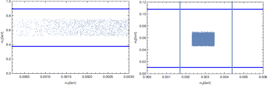
Figure 1: Correlations between the first and second generation SM quark
masses. The horizontal and vertical lines are the minimum and maximum values
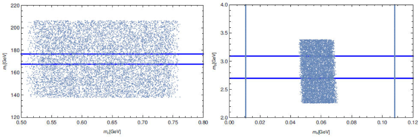
of the second and first generation quark masses, respectively, inside the experimentally allowed range.Figure 2: Correlations between the second and third generation SM quark
masses. The horizontal and vertical lines are the minimum and maximum values
of the third and second generation quark masses, respectively, inside the experimentally allowed range.
With the aim to study the sensitivity of the obtained values for the SM quark
masses under variations around the best-fit values (maximum variation
around the of their best fit values), we show in Figs. 1 and 2, the correlations between the first and second as well as between third and second generation SM quark masses. We have found that such variations yield values for the SM quark masses inside the experimentally allowed range, with the exception of the top and bottom quark masses where the majority of points are outside the range. Consequently the quark sector model parameters feature some moderate amount of fine tuning. We have numerically checked that the up and down type quark sector parameters have to be varied in range around the and of their best fit values, respectively, in order to obtain all SM quark masses inside their experimentally allowed range.
IV Lepton masses and mixings
The lepton fields and the corresponding scalars in lepton sectors, under the
, is given in Table 3.
The lepton Yukawa terms invariant under the symmetries of the model are:
(4)
In the case where is spontaneously broken down to by the VEVs alignment
and , within the following expansions
(5)
we get the lepton flavor changing interactions as follows
(6)
From (6), it follows that, in the model under consideration, the usual Yukawa couplings are associated with the factor
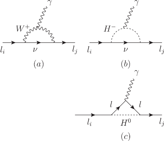
and the lepton flavor changing decays consist of the contribution of three Feynman diagrams as in Fig. 3.
Figure 3: Feynman diagrams contributing to lepton flavor changing decay. Here and and .
The current experimental data on lepton flavor changing decays read Olive:2016xmw : and .
The partial decay width is given by br1 ; br2
(7)
where the above form factors and are determined from the process amplitude br1 ; br2
(8)
For the case , we get
(9)
where .
In the model under consideration, one has br2 ; br3
(10)
where is the mass scale of the heavy scalars (which provide the dominant contributions to the LFV decays) running in the internal lines of the loop.
For further details on the form factors , the
reader is referred to Refs. br1 ; br2 ; br3 ; br4 .
Combining (9) and (10), we see that the lepton flavor changing processes in this model are suppressed by the factor associated with the above mentioned small Yukawa couplings and the large mass scale of the heavy scalars running in the internal lines of the loop.
Let us turn into lepton mass issue. From (4), the lepton mass terms read
(11)
where the mass matrix for charged leptons is given by:
(15)
This matrix can be diagonalized as,
(16)
where
(23)
(24)
where is the cube root of unity.
The best fit values for the masses of charged-leptons are given in Ref. PDG2018 : , , . Then, we find the relations .
We also assume that in the neutrino sector, the discrete group is spontaneously broken down to the Klein four group by the VEV alignment of and the VEVs of as . In this case, the neutrino mass matrices become
(25)
(26)
(33)
(40)
(47)
(54)
Let us note that the matrices given by Eqs. (25) - (54) are all symmetric and , , , , , are respectively generated from the renormalizable Yukawa interactions , , , , , , whereas and arise from the non-renormalizable Yukawa interactions and , respectively.
In this work, we introduce the symmetry111All the lepton fields and the corresponding scalars in Table 3 carry the same charged (+ 1) under which is not necessary to write out here., which in addition to the symmetry to prevent some Yukawa interactions thus giving rise to the predictive textures for the neutrino sector shown in Eqs. (25) - (54). For instance, since the product of two triplets contains a triplet, the coupling can transform under as , which implies that in order to generate the mass matrix , one needs one singlet transforming as (1, -1, 1,1,1,0), in order to build an invariant under all given symmetries. For the known scalars, is forbidden by the symmetry, is prevented by the symmetry, is not allowed by the and symmetries, whereas is forbidden by and symmetries and is prevented by the symmetry. Consequently, there is only one term involving the fields , and , invariant under the symmetry, which corresponds to as in Eq. (4) that provide a simple form of as indicated by Eq. (25). The situation is similar for the remaining couplings that generate the other mass matrices given in Eqs.(25) - (54).
In the basis ( , N, S), the full neutrino mass matrix predicted by our model takes the form:
(58)
The light active neutrino masses are obtained by diagonalizing the matrix given by Eq. (58) and this is done by introducing the following matrices
(63)
The effective neutrino mass matrix in Eq. (58) can be rewritten in the form:
(66)
which is similar to the one resulting from a type-I seesaw mechanism. Then, the light active neutrino mass matrix takes the form:
(67)
Replacing Eqs. (25) - (54) in Eq. (67) yields the following mass matrix for light active neutrinos:
(71)
where
(72)
(73)
with , and defined in Eqs. (25) - (54).
The mass matrix for light active neutrinos is diagonalized by the rotation matrix ,
(77)
and the light active neutrino masses are given by
(78)
By combining Eqs. (23) and (77) we find that the leptonic mixing matrix takes the form:
(82)
We see that all the elements of the matrix in Eq. (82) depend only on two parameters and . From
experimental constraints on the elements of the lepton mixing matrix given
in Ref. Uconstraint , we can find out the regions
of and to establish experimental constraints for lepton
mixing matrix.
In the standard Particle Data Group (PDG) parametrization, the leptonic mixing
matrix can be parameterized in three Euler’s angles as follows:
(83)
(84)
(85)
i.e, and in Eqs. (83) and (85) depend only on one parameter .
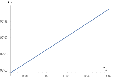
Eqs. (83) - (85) yields:
(86)
(87)
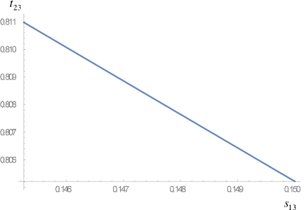
Figure 4: as a function of
with .Figure 5: as a function of
with .
The data in Particle Data Group 2018 PDG2018 shows that so and as depicted in Figs. 4 and 5, respectively. Taking the best fit value given in Ref. PDG2018 , we get ( and ( which are in good agreement with the values of and given in Ref. PDG2018 . On the other hand, with this best value of , we get and Dirac CP violation phase which is a viable value of the CP violating Dirac phase PDG2018 . The leptonic mixing matrix in Eq. (91) takes the explicit form
(91)
which is an unitary matrix.
The expression (91) shows that is free parameter so we can choose the VEV alignment in the charged-lepton sector as , i.e, may get the value . In this case, the leptonic mixing matrix becomes:
(95)
or
(99)
i.e, the ranges of the magnitude of the elements of the three-flavour
leptonic mixing matrix is consistent with those of given in Ref. Uconstraint .
At present, the values of neutrino masses (or the absolute neutrino
masses) as well as the mass ordering of neutrinos are still unknown. The result in Ref. Tegmark shows that while the upper bound on the sum of light active neutrino masses is given by constraint ,
(100)
The experimental neutrino oscillation data given in Eq. (1) are compatible with two possible signs of
which is currently unknown and correspond to two types of neutrino mass spectra.
IV.1 Normal spectrum ()
By taking the best fit values on neutrino mass squared differences for normal spectrum, given in Ref. PDG2018 ,
and , we obtain four solutions, however, they have the same absolute values of , the unique
difference is the sign of them. So, here we only consider the following solution:
(101)
where
(102)
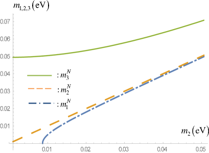
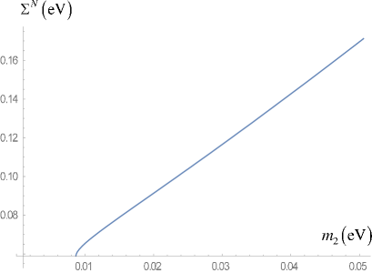
In the model under consideration, is a good region of that can reach the realistic normal neutrino mass
hierarchy which is depicted in Fig. 7. In the case , the parameters and the other neutrino masses are explicitly
given as , and which corresponds to a normal
neutrino mass spectrum. The sum of all three neutrino in this case is given by lying within the cosmological
bound from Planck data given in Eq. (100).
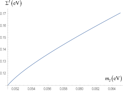
Figure 6: as functions of
with in the normal spectrum.Figure 7: as functions of
with in the normal spectrum.
IV.2 Inverted spectrum ()
Similar to the normal spectrum, by taking the best fit values on neutrino mass squared differences for inverted spectrum, given in Ref. PDG2018 ,
and , we get a solution as follows:
(103)
where
(104)
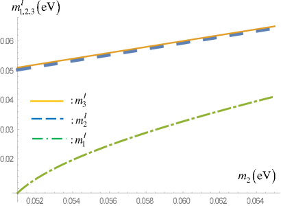
In this model, is a good region of that can reach the inverted neutrino mass hierarchy which is depicted in Fig. 8. In the case , the parameters and the other neutrino masses are explicitly
given as , and which corresponds to an inverted
neutrino mass spectrum. The sum of all three neutrino in this case is given by which is consistent with the cosmological
bound from Planck data in Eq.(100).
Figure 8: as functions of
with in the inverted spectrum.Figure 9: as functions of
with in the inverted spectrum.
V Conclusions
We have proposed a low-scale seesaw model to generate the masses for the active neutrinos based on flavour symmetry supplemented by the group,
where the masses of the SM charged fermions and the fermionic mixing angles are generated from a Froggatt-Nielsen mechanism after the spontaneous breaking of the group.
The obtained values for the physical observables of the quark and
lepton sectors are in good agreement with the most recent experimental data. The Dirac CP violating phase is predicted to be which is consistent with the most recent neutrino oscillation experimental data PDG2018 . The predictions for the absolute neutrino masses in the model can also saturate the recent constraints.
Acknowledgments
This research is funded by Vietnam National Foundation for Science and Technology Development (NAFOSTED) under grant number 103.01-2017.341 as well as by Fondecyt (Chile), Grants
No. 1170803, CONICYT PIA/Basal FB0821. H. N. L acknowledges the warm hospitality at BLTP, JINR and the financial support of the
Vietnam Academy of Science and Technology under grant NVCC05.01/19-19. A.E.C.H is very grateful to the Institute of Physics, Vietnam Academy
of Science and Technology for the warm hospitality.
References
(1) A. E. Cárcamo Hernández, Sergey Kovalenko, H. N. Long, and Ivan
Schmidt, J. High Energy Phys. 1807, 144 (2018), arXiv:1705.09169 [hep-ph] and references therein.
(2) M. Tanabashi et al. (Particle Data Group), Phys. Rev. D 98, 030001 (2018) and 2019 update.
(3) N. Cabibbo, Phys Rev. Lett. 10, 531 (1963).
(4) M. Kobayashi and T. Maskawa, Prog. Theor. Phys. 49, 652 (1973).
(5) Y. Cai, T. Han, T. Li, R. Ruiz, Front.in Phys. 6, 40 (2018).
(6) R. N. Mohapatra, Phys. Rev. Lett. 56, 561 (1986).
(7) R. N. Mohapatra, J. W. F. Valle, Phys. Rev. D34, 1642 (1986).
(8) M. Malinsky, J. C. Romao and J. W. F. Valle, Phys. Rev. Lett. 95, 161801 (2005) [arXiv: hep-ph/0506296].
(9) P. S. B. Dev, R. N. Mohapatra, Phys. Rev. D 81 (2010) 013001, arXiv:0910.3924 [hep-ph].
(10) S. S. C. Law, K. L. McDonald, Phys. Rev. D 87 (2013) 113003, arXiv:1303.4887 [hep-ph].
(11) B. Adhikary, A. Ghosal, P. Roy, Indian J. Phys. 88 (2014) 979, arXiv:1311.6746 [hep-ph].
(12) S. Fraser, E. Ma, O. Popov, Phys. Lett. B 737 (2014) 280, arXiv:1408.4785 [hep-ph].
(13) A. E. Cárcamo Hernández, I.d.M. Varzielas, J. Phys. G 42 (6) (2015) 065002, arXiv:1410.2481 [hep-ph].
(14) A. Abada and M. Lucente, Nucl. Phys. B 885, 651 (2014), arXiv: 1401.1507 [hep-ph].
(15) A. Ghosal, R. Samanta, J. High Energy Phys. 1505 (2015) 077, arXiv:1501.00916 [hep-ph].
(16) M. Chakraborty, H. Z. Devi, A. Ghosal, Phys. Lett. B 905 (2016) 337, arXiv:1501.05937 [hep-ph].
(17) A. E. Cárcamo Hernández, R. Martínez, F. Ochoa, Eur. Phys.J. C 76 (2016), 11, 634, arXiv:1309.6567 [hep-ph].
(18)R. Sinha, R. Samanta, A. Ghosal, Phys. Lett. B 759 (2016) 206, arXiv: 1508.05227 [hep-ph].
(19) M. Sruthilaya, R. Mohanta, S. Patra, Eur. Phys. J. C (2018) 78 : 719, arXiv: 1709.01737 [hep-ph].
(20) A. E. Cárcamo Hernández, S. Kovalenko, J. W. F. Valle and C. A. Vaquera-Araujo, J. High Energy Phys. 1707, 118 (2017), arXiv: 1705.06320 [hep-ph].
(21) D. Borah, B. Karmakar, Phys. Lett. B 789 (2019), 59, arXiv:1806.10685 [hep-ph].
(22) A. E. Cárcamo Hernández and H. N. Long, J. Phys. G 45, no. 4, 045001 (2018), arXiv:1705.05246 [hep-ph].
(23) A. E. Cárcamo Hernández, H. N. Long and V. V. Vien,
Eur. Phys. J. C 78, no. 10, 804 (2018), arXiv:1803.01636 [hep-ph].
(24) A. E. Cárcamo Hernández, Y. Hidalgo Velásquez and N. A. Pérez-Julve, arXiv:1905.02323 [hep-ph].
(25) A. E. Cárcamo Hernández and S. F. King, arXiv: 1903.02565 [hep-ph].
(26)
A. E. Cárcamo Hernández, S. Kovalenko, J. W. F. Valle and C. A. Vaquera-Araujo, J. High Energy Phys.1902, 065 (2019), arXiv:1811.03018 [hep-ph].
(27) A. E. Cárcamo Hernández, J. Marchant González and U. J. Saldaña-Salazar, Phys. Rev. D 100, no. 3, 035024 (2019), arXiv: 1904.09993 [hep-ph].
(28) A. E. Cárcamo Hernández, N. A. Pérez-Julve and Y. Hidalgo Velásquez, arXiv:1907.13083 [hep-ph].
(29) P. V. Dong, H. N. Long, C. H. Nam, and V. V. Vien, Phys. Rev. D 85, 053001(2012), arXiv: 1111.6360 [hep-ph].
(30)
K. Bora, Horizon 2, 112 (2013), arXiv: 1206.5909 [hep-ph].
(31) Z. z. Xing, H. Zhang and S. Zhou, Phys. Rev. D 77, 113016 (2008), arXiv:0712.1419 [hep-ph].
(32)
C. Patrignani et al. Particle Data Group), Chin. Phys. C 40, 100001 (2016).
(33) M. C. Gonzalez-Garcia, M. Maltoni, T. Schwetz, J. High Energy Phys. 1411, 052 (2014), arXiv: 1409.5439 [hep-ph].
(34) M. Tegmark et al., SDSS Collaboration, Phys. Rev. D 69 (2004) 103501, arXiv:astro-ph/0310723.