Double parton distributions in the pion
in the Nambu and Jona-Lasinio model

Abstract

Two-parton correlations in the pion, a non perturbative information encoded in double parton distribution functions, are investigated in the Nambu and Jona-Lasinio model. It is found that double parton distribution functions expose novel dynamical information on the structure of the pion, not accessible through one-body parton distributions, as it happens in several estimates for the proton target and in a previous evaluation for the pion, in a light-cone framework. Expressions and predictions are given for double parton distributions corresponding to leading-twist Dirac operators in the quark vertices, and to different regularization methods for the Nambu and Jona-Lasinio model. These results are particularly relevant in view of forthcoming lattice data.

1 Introduction

Since the start of the LHC operation, multiple parton interactions (MPI) have become an important topic in nowadays hadronic Physics [1]. Due to the high partonic densities reached, processes where more than two partons from the two colliding protons participate in the actual scattering process are likely to happen. The simplest form of MPI, double parton scattering (DPS), involving two simultaneous hard collisions, has been indeed observed at the LHC (see, e.g., Ref. [2]). The DPS cross section is written in terms of double parton distribution functions (dPDFs) [3, 4], related to the number density of two partons, with given longitudinal momentum fractions, located at a given transverse separation in coordinate space. These distributions encode information complementary to that obtained through the tomography, accessed using electromagnetic probes, in terms of generalized parton distributions (GPDs) [5, 6]. If measured, dPDFs would therefore represent a novel tool to study the three-dimensional hadron structure [7, 8, 9, 10]. Indeed, they are sensitive to two-parton correlations not accessible via one body distributions, i.e. standard partons distribution functions (PDFs) and GPDs (see Ref. [11] for a recent report). Since dPDFs describe soft Physics, they are non perturbative objects and have not been evaluated in QCD. It is therefore useful to estimate them at low momentum scales ($\sim\Lambda_{QCD}$), using models of the hadron structure, as it has been proposed, for the proton, in Refs. [12, 13, 14, 15, 16, 17, 18]. In order to match theoretical predictions with future experimental analyses, the results of these calculations are then evolved using perturbative QCD to reach the high momentum scale of the data. Evolution properties of dPDFs have been studied in the past [19, 20] and have been recently object of deep investigation (for new developments see, e.g., the report [21]).

Recently, results have been obtained for two current correlations in the pion on the lattice [22, 23], quantities related to dPDFs, whereas the corresponding evaluation for the nucleon appears much more involved. The novel possibility to compare results with lattice data makes model calculations of pion dPDFs of relevant theoretical interest. A first estimate of pion dPDFs has been performed in Ref. [24], using light cone wave functions obtained within the AdS/QCD correspondence.

In this paper we analyze pion dPDFs within a Nambu–Jona-Lasinio (NJL) framework [25].

The dependence of the results on the possible choice of regularization of the NJL model is investigated within two different prescriptions, the standard Pauli–Villars one and a properly built Light Front regularization. Our aim is the first evaluation of pion dPDFs in a field theoretical approach which allows to study systematically different contributions. This procedure is useful, e.g., to check the validity of approximated expressions for dPDFs in terms of GPDs, and to calculate quantities related to two current correlations in the pion, towards a direct comparison with lattice data.

The paper is structured as follows. In section 2 we define the pion dPDFs, we describe the NJL evaluation scheme and show the results of the calculation. In section 3 we test the validity, within our scheme, of a commonly used approximation of the dPDF in terms of GPDs. Conclusions are collected in section 4.

2 Double parton distribution functions in the pion

For the definition of the quantities to be evaluated, we follow the conventions introduced in Ref. [4]. In particular, a dPDF for the pion is defined as

$$F_{a_{1},\bar{a}_{2}}(x_{1},x_{2},\vec{y}_{\perp})=\int d^{2}k_{1\perp}d^{2}k_{2\perp}F_{a_{1},\bar{a}_{2}}(x_{1},x_{2},\vec{k}_{1\perp},\vec{k}_{2\perp},\vec{y}_{\perp})~{},$$ (1)

with $\vec{y}_{\perp}$ the transverse distance between the two partons, starting from the generic light-cone correlator

$$F_{a_{1},\bar{a}_{2}}(x_{1},x_{2},\vec{k}_{1\perp},\vec{k}_{2\perp},\vec{y}_{\perp}) = -2P^{+}\int\frac{dz_{1}^{-}d^{2}z_{1\perp}}{(2\pi)^{3}}\frac{dz_{2}^{-}d^{2}z_{2\perp}}{(2\pi)^{3}}e^{ix_{1}z_{1}^{-}P^{+}-i\vec{z}_{1\perp}\cdot\vec{k}_{1\perp}}$$ (2)

$$\times e^{ix_{2}z_{2}^{-}P^{+}-i\vec{z}_{2\perp}\cdot\vec{k}_{2\perp}}\,{\cal{O}}_{a_{1}\bar{a}_{2}}~{},$$

where

$${\cal{O}}_{a_{1},\bar{a}_{2}} = \int dy^{-}\,\left\langle\pi^{i}\left(P\right)\right|\left\{\left[\bar{q}\left(\tfrac{1}{2}z_{2}\right)\bar{\Gamma}_{\bar{a}_{2}}q\left(-\tfrac{1}{2}z_{2}\right)\right]\right.$$ (3)

$$\times \left.\left[\bar{q}\left(y-\tfrac{1}{2}z_{1}\right)\bar{\Gamma}_{a_{1}}q\left(y+\tfrac{1}{2}z_{1}\right)\right]\right\}_{z_{1}^{+}=z_{2}^{+}=y^{+}=0}\left|\pi^{i}\left(P\right)\right\rangle\,,$$

with $i$ the isospin index of the pion. In the equations above, the index $a_{1}\,\left(\bar{a}_{2}\right)$ is a short notation for the Dirac and isospin indices associated to the matrices involved in the quark (antiquark) vertex:

$$\bar{\Gamma}_{a_{1}}=\Gamma_{a_{1}}\,\tau^{a_{1}}\,,$$ (4)

with $\Gamma_{a_{1}}$ given by

$$\Gamma_{q} = \Gamma_{\bar{q}}=\frac{1}{2}\gamma^{+}~{},\quad\quad\quad\quad\Gamma_{\Delta_{q}}=-\Gamma_{\Delta\bar{q}}=\frac{1}{2}\gamma^{+}\gamma_{5}~{},$$

$$\Gamma_{\delta_{q}}^{i} = \Gamma_{\delta\bar{q}}^{i}=\frac{1}{2}i\sigma^{i+}\gamma_{5}~{},$$ (5)

in the vector, axial and tensor sectors, related to leading twist distributions, respectively.

We follow Ref. [4] to analyze the structure of the dPDFs. The functions $F_{q,\bar{q}}\left(x_{1},x_{2},y_{\perp}\right)$ and $F_{\Delta q,\Delta\bar{q}}\left(x_{1},x_{2},y_{\perp}\right)$ are, by construction, scalar quantities and, therefore, functions of $y_{\perp}=\left|\vec{y}_{\perp}\right|$. The two functions $F_{q,\Delta\bar{q}}\left(x_{1},x_{2},y_{\perp}\right)$ and $F_{\Delta q,\bar{q}}\left(x_{1},x_{2},y_{\perp}\right)$ vanish identically, for parity conservation. Four dPDFs turn out to be two-dimensional vectors in the transverse plane. They can be written in terms of scalar functions, as follows

$$\begin{array}[]{ccc}F_{q,\delta\bar{q}^{j}}\left(x_{1},x_{2},\vec{y}_{\perp}\right)=\epsilon^{j,k}\,\hat{y}^{k}_{\perp}\,F_{q,\delta\bar{q}}^{v}\left(x_{1},x_{2},y_{\perp}\right)\,,&&F_{\delta q^{j},\bar{q}}\left(x_{1},x_{2},\vec{y}_{\perp}\right)=\epsilon^{j,k}\,\hat{y}^{k}_{\perp}\,F_{\delta q,\bar{q}}^{v}\left(x_{1},x_{2},y_{\perp}\right)\quad,\\ \\ F_{\Delta q,\delta\bar{q}^{j}}\left(x_{1},x_{2},\vec{y}_{\perp}\right)=\hat{y}^{j}_{\perp}\,F_{\Delta q,\delta\bar{q}}^{v}\left(x_{1},x_{2},y_{\perp}\right)\,,&&F_{\delta q^{j},\Delta\bar{q}}\left(x_{1},x_{2},\vec{y}_{\perp}\right)=\hat{y}^{j}_{\perp}\,F_{\delta q,\Delta\bar{q}}^{v}\left(x_{1},x_{2},y_{\perp}\right)\quad.\end{array}$$ (6)

The last dPDF is a tensor quantity and, in terms of scalar functions, it reads

$$F_{\delta q^{j},\delta\bar{q}^{k}}\left(x_{1},x_{2},\vec{y}_{\perp}\right)=\delta^{j,k}\,F_{\delta q,\delta\bar{q}}^{s}\left(x_{1},x_{2},y_{\perp}\right)+\left(2\hat{y}^{j}_{\perp}\,\hat{y}^{k}_{\perp}-\delta^{j,k}\right)\,F_{\delta q,\delta\bar{q}}^{t}\left(x_{1},x_{2},y_{\perp}\right)\quad,$$ (7)

with $\hat{y}_{\perp}=\vec{y}_{\perp}/\left|\vec{y}_{\perp}\right|$.

It is convenient to calculate the dPDFs in momentum space,

$$F_{a_{1},\bar{a}_{2}}(x_{1},x_{2},\vec{q}_{\perp})=\int d^{2}k_{1\perp}d^{2}k_{2\perp}d^{2}y_{\perp}e^{i\,\vec{y}_{\perp}\cdot\vec{q}_{\perp}}F_{a_{1},\bar{a}_{2}}(x_{1},x_{2},\vec{k}_{1\perp},\vec{k}_{2\perp},\vec{y}_{\perp})~{},$$ (8)

a quantity often called “2GPD” [7, 8] which, at variance with the dPDF Eq. (1), is not related to a probability density. The natural support in $x_{1,2}$ of the function $F_{q_{1}\bar{q}_{2}}$ is $0\leq x_{1,2}\leq 1$, $0\leq x_{1}+x_{2}\leq 1$. The quantity $\vec{q}_{\perp}$ represents the imbalance between the relative momentum of the two partons in the considered hadronic state and in its conjugated one.

Expressions equivalent to Eqs. (6) and (7), yielding vector and tensor quantities in terms of scalar functions, can be given in momentum space as follows

$$\begin{array}[]{ccc}F_{q,\delta\bar{q}^{j}}\left(x_{1},x_{2},\vec{q}_{\perp}\right)=i\,\epsilon^{j,k}\,\hat{q}^{k}_{\perp}\,F_{q,\delta\bar{q}}^{v}\left(x_{1},x_{2},q_{\perp}\right)\,,&&F_{\delta q^{j},\bar{q}}\left(x_{1},x_{2},\vec{q}_{\perp}\right)=i\,\epsilon^{j,k}\,\hat{q}^{k}_{\perp}\,F_{\delta q,\bar{q}}^{v}\left(x_{1},x_{2},q_{\perp}\right)\quad,\\ \\ F_{\Delta q,\delta\bar{q}^{j}}\left(x_{1},x_{2},\vec{q}_{\perp}\right)=i\,\hat{q}^{j}_{\perp}\,F_{\Delta q,\delta\bar{q}}^{v}\left(x_{1},x_{2},q_{\perp}\right)\quad,&&F_{\delta q^{j},\Delta\bar{q}}\left(x_{1},x_{2},\vec{q}_{\perp}\right)=i\,\hat{q}^{j}_{\perp}\,F_{\delta q,\Delta\bar{q}}^{v}\left(x_{1},x_{2},q_{\perp}\right)\quad,\end{array}$$

$$F_{\delta q^{j},\delta\bar{q}^{k}}\left(x_{1},x_{2},\vec{q}_{\perp}\right)=\delta^{j,k}\,F_{\delta q,\delta\bar{q}}^{s}\left(x_{1},x_{2},q_{\perp}\right)+\left(2\hat{q}^{j}_{\perp}\,\hat{q}^{k}_{\perp}-\delta^{j,k}\right)\,F_{\delta q,\delta\bar{q}}^{t}\left(x_{1},x_{2},q_{\perp}\right)\,\,\,.$$ (9)

By evaluating the Fourier transformations, Eq. (8) for the scalar, vector and tensor quantities, the scalar functions $F_{a_{1},\bar{a}_{2}}\left(x_{1},x_{2},y_{\perp}\right)$ in coordinate space are found to be related to the scalar functions $F_{a_{1},\bar{a}_{2}}\left(x_{1},x_{2},q_{\perp}\right)$ in momentum space according to expressions given here below. In the case of the scalar quantities $F_{q,\bar{q}}\left(x_{1},x_{2},q_{\perp}\right)$, $F_{\Delta q,\Delta\bar{q}}\left(x_{1},x_{2},q_{\perp}\right)$ and $F_{\delta q,\delta\bar{q}}^{s}\left(x_{1},x_{2},q_{\perp}\right),$ one gets

$$F_{a_{1},\bar{a}_{2}}\left(x_{1},x_{2},y_{\perp}\right)=\int\,\frac{dq_{\perp}\,q_{\perp}}{2\pi}J_{0}\left(q_{\perp}y_{\perp}\right)\,F_{a_{1},\bar{a}_{2}}\left(x_{1},x_{2},q_{\perp}\right)\,\,.$$ (10)

For the scalar functions defining the vector quantities, $F_{q,\delta\bar{q}}^{v}\left(x_{1},x_{2},q_{\perp}\right)$, $F_{\delta q,\bar{q}}^{v}\left(x_{1},x_{2},q_{\perp}\right)$
$F_{\Delta q,\delta\bar{q}}^{v}\left(x_{1},x_{2},q_{\perp}\right)$ and $F_{\delta q,\Delta\bar{q}}^{v}\left(x_{1},x_{2},q_{\perp}\right)$, one has

$$F_{a_{1},\bar{a}_{2}}^{v}\left(x_{1},x_{2},y_{\perp}\right)=\int\,\frac{dq_{\perp}\,q_{\perp}}{2\pi}J_{1}\left(q_{\perp}y_{\perp}\right)F_{a_{1},\bar{a}_{2}}^{v}\left(x_{1},x_{2},q_{\perp}\right)\,\,,$$ (11)

and, for the scalar function present in the tensor structure, $F_{\delta q,\delta\bar{q}}^{t}\left(x_{1},x_{2},q_{\perp}\right)$, the relation is

$$F_{\delta q,\delta\bar{q}}^{t}\left(x_{1},x_{2},y_{\perp}\right)=-\int\,\frac{dq_{\perp}\,q_{\perp}}{2\pi}J_{2}\left(q_{\perp}y_{\perp}\right)F_{\delta q,\delta\bar{q}}^{t}\left(x_{1},x_{2},q_{\perp}\right)\,\,.$$ (12)

The calculation framework is the NJL model, the most realistic model for the pseudoscalar mesons based on a local quantum field theory built with quarks [25]. It respects the realization of chiral symmetry and gives a good description of low energy properties. Mesons are described as bound states, in a fully covariant fashion, using the Bethe-Salpeter amplitude, in a field theoretical framework. In this way, Lorentz covariance is preserved. The NJL model is a non-renormalizable field theory and therefore a regularization procedure has to be implemented. We have performed initially our calculations in the Pauli- Villars ($PV$) regularization scheme, which is a well established method. The NJL model, together with its regularization procedure, can be regarded as an effective theory of QCD. Some basic features of the NJL model and details on the regularization schemes are reported in Appendix A.

Model calculations of meson partonic structure within this approach have a long story of successful predictions [26, 27, 28, 30, 29, 31, 32, 33, 34, 35, 36].

One should remember that collinear parton distributions obtained within a model have to be associated to a low momentum scale $Q_{0}^{2}$, at which one has only valence quarks, and, in order to be used to predict measured quantities, have to be evolved to higher momentum scales according to perturbative QCD (pQCD).

Let us describe the main steps of the calculation of Eq. (8) in the NJL model. For the pion $i$ we use the state

$$\left|\pi^{i}\left(P\right)\right\rangle=\int d^{4}y_{1}\,d^{4}y_{2}\,\frac{d^{4}k}{\left(2\pi\right)^{4}}e^{-i\frac{1}{2}P\cdot\left(y_{1}+y_{2}\right)}\,e^{-ik\cdot\left(y_{1}-y_{2}\right)}\bar{q}\left(y_{1}\right)\phi_{\pi^{i}}\left(k,P\right)q\left(y_{2}\right)\left|0\right\rangle\,,$$ (13)

with $\phi_{\pi^{i}}$ the quark-pion vertex function for a $\pi^{i}$. In the NJL model the amplitude $\phi_{\pi^{i}}\left(k,P\right)$ is independent on the relative and total quark-antiquark momenta, $k$ and $P,$ respectively, and we have

$$\phi_{\pi^{i}}\left(k,P\right)=ig_{\pi qq}i\gamma_{5}\tau^{i}$$ (14)

where $g_{\pi qq}$ is the quark-pion coupling constant and $\tau^{i}$ is the isospin matrix associated to the corresponding pion $\pi^{i}$.

Let us consider the case of a $\pi^{+}$, and therefore the operators $\bar{\Gamma}_{a}=\Gamma_{a}\frac{1}{2}(1+\tau_{3})$ and $\bar{\Gamma}_{\bar{a}}=\Gamma_{\bar{a}}\frac{1}{2}(1-\tau_{3})$. At leading order, we have the contribution depicted in Fig 1. Using Eqs. (13) and (14) in Eq. (3), after a tedious but straightforward calculation we get, for the momentum space dPDF Eq. (8),

$$F_{a_{1},\bar{a_{2}}}\left(x_{1},x_{2},\vec{q}_{\perp}\right) =-2P^{+}\int\frac{d^{4}k}{\left(2\pi\right)^{4}}\frac{dq^{-}}{2\pi}\delta\left(P^{+}x_{1}-\frac{1}{2}\left(P+2k\right)^{+}\right)\,\delta\left(P^{+}x_{2}+\frac{1}{2}\left(-P+2k\right)^{+}\right)$$

$$\left(-\right)\text{Tr}\left[iS_{F}\left(\frac{P}{2}+k-\frac{q}{2}\right)\,\phi_{\pi^{+}}\,iS_{F}\left(-\frac{P}{2}+k-\frac{q}{2}\right)\,\bar{\Gamma}_{\bar{a_{2}}}\,iS_{F}\left(-\frac{P}{2}+k+\frac{q}{2}\right)\right.$$

$$\times\left.\bar{\phi}_{\pi^{+}}\,iS_{F}\left(\frac{P}{2}+k+\frac{q}{2}\right)\bar{\Gamma}_{a_{1}}\right]\,,$$ (15)

where

$$\bar{\phi}_{\pi^{+}}\left(k,P\right)=-\gamma_{0}\,\phi_{\pi^{+}}^{\dagger}\left(k,P\right)\,\gamma_{0}~{},$$ (16)

and the quark propagator is given by $S_{F}(k)=(\cancel{k}-m+i\epsilon)^{-1}$ and the trace is intended in color, isospin and quadri-spinor indices.

Figure 1: Diagram of the Double Parton Distribution Function associated to Eq. (15). Open vertices represent nonlocal current insertions.

We observe that this contribution can be obtained defining

$$F_{a_{1},\bar{a_{2}}}\left(x_{1},x_{2},\vec{q}_{\perp}\right)=-2P^{+}\int\frac{dq^{-}}{2\pi}\,\mathcal{T}\,,$$ (17)

where $\mathcal{T}$ is the Feynman amplitude corresponding to the diagram of Fig. 1, $q^{\mu}=\left(0,\vec{q}_{\perp},q^{-}\right)$ and the following bilocal current vertex has to be used:

$\Rightarrow$

$\bar{\Gamma}_{a_{1}}\,\delta\left(P^{+}x_{1}-\frac{1}{2}\left(p_{1}+p_{2}\right)^{+}\right)$

$\Rightarrow$

$\bar{\Gamma}_{\bar{a}_{2}}\,\delta\left(P^{+}x_{2}+\frac{1}{2}\left(p_{1}+p_{2}\right)^{+}\right)$

Table 1: Bare vertices associated to the bilocal currents.

The integration over the $k^{+}$ variable in Eq. (15) using the Dirac delta, and the integration over $k^{-}$ and $q^{-}$ using the Cauchy theorem of residues, give

$$F_{a_{1},\bar{a_{2}}}\left(x_{1},x_{2},\vec{q}_{\perp}\right)=\delta\left(x_{1}+x_{2}-1\right)\,\theta\left(x_{1}\right)\,\theta\left(1-x_{1}\right)\left(-\frac{N_{c}\,g_{\pi qq}^{2}}{2\pi P^{+2}}\right)$$ (18)

$$\int\frac{d^{2}k_{\perp}}{\left(2\pi\right)^{2}}\frac{tr_{a_{1},\bar{a}_{2}}\left(\vec{k}_{\perp},\vec{q}_{\perp}\right)}{\left[\left(\vec{k}_{\perp}-\frac{q_{\perp}}{2}\right)^{2}+m^{2}-x_{1}\left(1-x_{1}\right)m_{\pi}^{2}-i\epsilon\right]\left[\left(\vec{k}_{\perp}+\frac{q_{\perp}}{2}\right)^{2}+m^{2}-x_{1}\left(1-x_{1}\right)m_{\pi}^{2}-i\epsilon\right]}\,,$$

with

$$tr_{a_{1},\bar{a_{2}}}\left(\vec{k}_{\perp},\vec{q}_{\perp}\right) = tr\left[\left(\frac{\cancel{P}}{2}+\cancel{k}-\frac{\cancel{q}}{2}+m\right)\gamma_{5}\left(-\frac{\cancel{P}}{2}+\cancel{k}-\frac{\cancel{q}}{2}+m\right)\Gamma_{\bar{a}_{2}}\right.$$ (19)

$$\times \left.\left(-\frac{\cancel{P}}{2}+\cancel{k}+\frac{\cancel{q}}{2}+m\right)\gamma_{5}\left(\frac{\cancel{P}}{2}+\cancel{k}+\frac{\cancel{q}}{2}+m\right)\Gamma_{a_{1}}\right]\,,$$

where $tr$ implies trace over quadri-spinors indices. Besides, we have

$$k^{\mu}=\left(\left(x_{1}-\frac{1}{2}\right)P^{+},\vec{k}_{\perp},\frac{P^{-}}{2}-\frac{m^{2}+\vec{k}_{\perp}^{\,2}}{2P^{+}\left(1-x_{1}\right)}\right)\,,$$ (20)

$$q^{\mu} =\left(0,\,\vec{q}_{\perp},\,\frac{-\vec{k}_{\perp}\cdot\vec{q}_{\perp}}{P^{+}\left(1-x_{1}\right)}\right)\,,$$ (21)

and $P^{2}=2P^{+}P^{-}=m_{\pi}^{2}.$

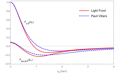
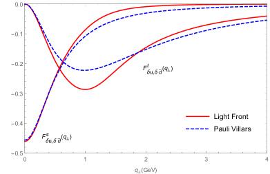
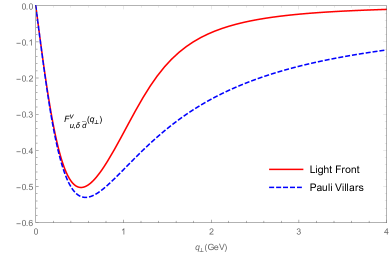
Figure 2: Double parton distribution functions in the NJL model, in momentum space, integrated over $x_{1},x_{2}$. Dashed (full) curves represent results obtained using the Pauli-Villars (Light-Front) regularization method. Top panel: quantities obtained integrating $F_{u,\bar{d}}\left(x_{1},x_{2},q_{\perp}\right)$, Eq. (22) (Eq. (32)) and $F_{\Delta u,\Delta\bar{d}}\left(x_{1},x_{2},q_{\perp}\right)$, Eq. (23) (Eq. (33)); central panel: quantities obtained integrating $F_{\delta u,\delta\bar{d}}^{s}\left(x_{1},x_{2},q_{\perp}\right)$, Eq. (25) (Eq. (35)) and $F_{\delta u,\delta\bar{d}}^{t}\left(x_{1},x_{2},q_{\perp}\right)$, Eq. (26) (Eq. (36)); bottom panel: the quantity obtained integrating $F_{u,\delta\bar{d}}^{v}\left(x_{1},x_{2},q_{\perp}\right)$, Eq. (27) (Eq. (37)).

The integral over $k_{\perp}$ present in Eq (18) is then rendered finite using the adopted Pauli-Villars regularization method, described in the Appendix A.2. Some intermediate steps are given in Appendix A.4. Our final results for the scalar functions appearing in the dPDFs related to different Dirac structures in the quark vertices are

$$F_{u,\bar{d}}^{\left(PV\right)}\left(x_{1},x_{2},q_{\perp}\right)=C(x_{1},x_{2})\,\sum_{j=0}^{2}c_{j}\,\left\{-\ln\frac{\kappa_{j}}{\kappa}+\left[2\frac{m_{\pi}^{2}}{q_{\perp}^{2}}x_{1}(1-x_{1})-1\right]f\left(\frac{\kappa_{j}}{q_{\perp}^{2}}\right)\right\}\,,$$ (22)

$$F_{\Delta u,\Delta\bar{d}}^{\left(PV\right)}\left(x_{1},x_{2},q_{\perp}\right)=C(x_{1},x_{2})\,\sum_{j=0}^{2}c_{j}\,\left\{-\ln\frac{\kappa_{j}}{\kappa}-\left[4\frac{m^{2}}{q_{\perp}^{2}}-2\frac{m_{\pi}^{2}}{q_{\perp}^{2}}x_{1}(1-x_{1})+1\right]f\left(\frac{\kappa_{j}}{q_{\perp}^{2}}\right)\right\}\,,$$ (23)

$$F_{u,\Delta\bar{d}}^{\left(PV\right)}\left(x_{1},x_{2},q_{\perp}\right)=F_{\Delta u,\bar{d}}^{\left(PV\right)}\left(x_{1},x_{2},q_{\perp}\right)=0$$ (24)

$$F_{\delta u,\delta\bar{d}}^{s\left(PV\right)}\left(x_{1},x_{2},q_{\perp}\right)=-C(x_{1},x_{2})\,\sum_{j=0}^{2}c_{j}\,2\frac{m^{2}}{q_{\perp}^{2}}f\left(\frac{\kappa_{j}}{q_{\perp}^{2}}\right)\,,$$ (25)

$$F_{\delta u,\delta\bar{d}}^{t\left(PV\right)}\left(x_{1},x_{2},q_{\perp}\right)=C(x_{1},x_{2})\,\sum_{j=0}^{2}c_{j}\,2\frac{\kappa_{j}}{q_{\perp}^{2}}f\left(\frac{\kappa_{j}}{q_{\perp}^{2}}\right)\,,$$ (26)

$$F_{u,\delta\bar{d}}^{v\left(PV\right)}\left(x_{1},x_{2},q_{\perp}\right)=-F_{\delta u,\bar{d}}^{v\left(PV\right)}\left(x_{1},x_{2},q_{\perp}\right)=-C(x_{1},x_{2})\,\sum_{j=0}^{2}c_{j}\,2\frac{m}{q_{\perp}}f\left(\frac{\kappa_{j}}{q_{\perp}^{2}}\right)\,.$$ (27)

$$F_{\Delta u,\delta\bar{d}}^{v\left(PV\right)}\left(x_{1},x_{2},q_{\perp}\right)=-F_{\delta u,\Delta\bar{d}}^{v\left(PV\right)}\left(x_{1},x_{2},q_{\perp}\right)=0$$ (28)

where $\kappa=m^{2}-m_{\pi}^{2}x_{1}(1-x_{1})$, $\kappa_{j}=M_{j}^{2}-m_{\pi}^{2}x_{1}(1-x_{1})$ and

$$C(x_{1},x_{2}) = \left(\frac{N_{c}\,g_{\pi qq}^{2}}{4\pi^{2}}\right)\delta\left(x_{1}+x_{2}-1\right)\,\theta\left(x_{1}\right)\,\theta\left(1-x_{1}\right)\,,$$ (29)

$$f(a) = \frac{1}{\sqrt{4a+1}}\,\log\frac{\sqrt{4a+1}+1}{\sqrt{4a+1}-1}\quad.$$ (30)

In the case of Eqs. (24) and (28), the traces involved in Eq. (19) are linear in the integrated momentum, $\vec{k}_{\perp},$ and, therefore, the corresponding dPDFs vanish after the integration present in Eq. (18). In ref. [4], as reported before in this section, the result of Eqs. (24) is predicted according to parity arguments.

One should notice first of all that, as expected by the Gaunt sum rule at $q_{\perp}^{2}=0$ [37], the $x_{2}$ integral yields the expression for the parton distribution function (PDF) reported, in the same NJL framework with Pauli-Villars regularization, in Refs. [27, 31].

We are now in the position to show our results for the pion dPDF for the $\pi^{+}$, in the NJL model. The dashed lines in Fig. 2 represent the quantities

$$F_{a_{1}\bar{a}_{2}}^{(PV)}\left({q}_{\perp}\right)=\int dx_{1}dx_{2}F_{a_{1}\bar{a}_{2}}^{(PV)}\left(x_{1},x_{2},{q}_{\perp}\right)\,,$$ (31)

where $F_{a_{1}\bar{a_{2}}}^{\left({PV}\right)}\left(x_{1},x_{2},{q}_{\perp}\right)$ is the generic scalar function used to define the momentum space dPDFs in Eqs. (9).

We show the results also in coordinate space, obtained by integrating over $x_{1},x_{2}$ the scalar functions defined in Eqs. (10)- (12). These quantities, multiplied by $y_{\perp}$, are given by the dashed lines in Fig. 3.

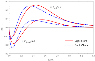
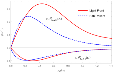
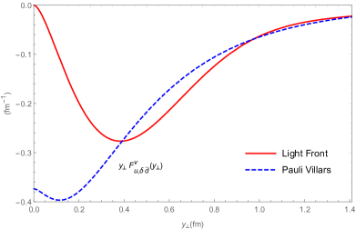
Figure 3: As in Fig. 2, but in transverse coordinate space

A few relevant comments are in order.

As stated in the Introduction, the scalar quantity $F_{u,\bar{d}}^{\left(PV\right)}\left(y_{\perp}\right)$, should represent, in principle, the probability density to have the two particles at a given transverse distance $y_{\perp}$. Indeed, our result for this function is properly normalized, as it can be read from Fig. 2 ($F_{u\bar{d}}^{\left(PV\right)}\,(q_{\perp}=0)=1$). Nonetheless it is found that $F_{u\bar{d}}^{\left(PV\right)}(y_{\perp})$ turns out to be negative at low values of $y_{\perp}$.

Another peculiar-looking feature of the results is related to the function $F_{u,\delta\bar{d}}^{v}\left(q_{\perp}\right)$. This quantity presents a slowly decreasing tail at high values of $q_{\perp}$, which produces in coordinate space a peculiar behavior at low values of $y_{\perp}$.

As these features are model dependent, one could wonder to what extent they are affected by the choice of the regularization scheme, as part of the model. For this reason we have performed the calculation using another, novel regularization procedure, suitable for calculation involving light-cone variables. This method, called here after Light Front (LF) regularization, is carefully described in Appendix A.3. Some intermediate results are included in Appendix A.4.

Our final results in the LF scheme are

$$F_{u,\bar{d}}^{\left(LF\right)}\left(x_{1},x_{2},q_{\perp}\right)=\tilde{C}(x_{1},x_{2})\,\left[g_{2}\left(q_{\perp}\right)+\left(\frac{\tilde{m}^{2}}{q_{\perp}^{2}}-\frac{1}{4}\right)\,g_{0}\left(q_{\perp}\right)\right]\,,$$ (32)

$$F_{\Delta u,\Delta\bar{d}}^{\left(LF\right)}\left(x_{1},x_{2},q_{\perp}\right)=\tilde{C}(x_{1},x_{2})\,\left[g_{2}\left(q_{\perp}\right)-\left(\frac{\tilde{m}^{2}}{q_{\perp}^{2}}+\frac{1}{4}\right)\,g_{0}\left(q_{\perp}\right)\right]\,,$$ (33)

$$F_{u,\Delta\bar{d}}^{\left(LF\right)}\left(x_{1},x_{2},q_{\perp}\right)=F_{\Delta u,\bar{d}}^{\left(LF\right)}\left(x_{1},x_{2},q_{\perp}\right)=0$$ (34)

$$F_{\delta u,\delta\bar{d}}^{s\left(LF\right)}\left(x_{1},x_{2},q_{\perp}\right)=-\tilde{C}(x_{1},x_{2})\,\frac{\tilde{m}^{2}}{q_{\perp}^{2}}\,g_{0}\left(q_{\perp}\right)\,,$$ (35)

$$F_{\delta u,\delta\bar{d}}^{t\left(LF\right)}\left(x_{1},x_{2},q_{\perp}\right)=-\tilde{C}(x_{1},x_{2})\,\left[g_{2}\left(q_{\perp}\right)-2\,\tilde{g}_{2}\left(q_{\perp}\right)+\frac{1}{4}\,g_{0}\left(q_{\perp}\right)\right]\,,$$ (36)

$$F_{u,\delta\bar{d}}^{v\left(LF\right)}\left(x_{1},x_{2},q_{\perp}\right)=-F_{\delta u,\bar{d}}^{v\left(LF\right)}\left(x_{1},x_{2},q_{\perp}\right)=-\tilde{C}(x_{1},x_{2})\,\frac{\tilde{m}}{q_{\perp}}\,g_{0}\left(q_{\perp}\right)\,.$$ (37)

$$F_{\Delta u,\delta\bar{d}}^{v\left(LF\right)}\left(x_{1},x_{2},q_{\perp}\right)=-F_{\delta u,\Delta\bar{d}}^{v\left(LF\right)}\left(x_{1},x_{2},q_{\perp}\right)=0$$ (38)

with $\tilde{\kappa}=\tilde{m}^{2}-m_{\pi}^{2}x_{1}(1-x_{1})$ and

$$\tilde{C}(x_{1},x_{2})=\left(\frac{N_{c}\,\tilde{g}_{\pi qq}^{2}}{4\pi^{2}}\right)\delta\left(x_{1}+x_{2}-1\right)\,\theta\left(x_{1}\right)\,\theta\left(1-x_{1}\right)\,,$$ (39)

$$g_{0}\left(q_{\perp}\right)=2\sqrt{\frac{q_{\perp}^{2}}{4\tilde{\kappa}+q_{\perp}^{2}}}\log\left(\frac{\left(\sqrt{4\tilde{\kappa}+q_{\perp}^{2}}+\sqrt{q_{\perp}^{2}}\right)\left(4\tilde{\kappa}+4\Lambda_{\perp}^{2}+q_{\perp}^{2}\right)}{\sqrt{q_{\perp}^{2}}\left(4\tilde{\kappa}-4\Lambda_{\perp}^{2}+q_{\perp}^{2}\right)+\sqrt{4\tilde{\kappa}+q_{\perp}^{2}}\sqrt{\left(4\tilde{\kappa}+4\Lambda_{\perp}^{2}-q_{\perp}^{2}\right)^{2}+16\tilde{\kappa}q_{\perp}^{2}}}\right)\,,$$ (40)

$$g_{2}\left(q_{\perp}\right)=-\frac{4\tilde{\kappa}+q_{\perp}^{2}}{4q_{\perp}^{2}}g_{0}\left(q_{\perp}\right)+\log\left(\frac{4\tilde{\kappa}+4\Lambda_{\perp}^{2}+\sqrt{\left(4\tilde{\kappa}+4\Lambda_{\perp}^{2}-q_{\perp}^{2}\right)^{2}+16\tilde{\kappa}q_{\perp}^{2}}-q_{\perp}^{2}}{8\tilde{\kappa}}\right)\,,$$ (41)

$$\tilde{g}_{2}\left(q_{\perp}\right) =\frac{-4\tilde{\kappa}-4\Lambda_{\perp}^{2}+\sqrt{\left(4\tilde{\kappa}+4\Lambda_{\perp}^{2}-q_{\perp}^{2}\right)^{2}+16\tilde{\kappa}q_{\perp}^{2}}-q_{\perp}^{2}}{4q_{\perp}^{2}}$$

$$+\frac{1}{2}\log\left(\frac{4\tilde{\kappa}+4\Lambda_{\perp}^{2}+\sqrt{\left(4\tilde{\kappa}+4\Lambda_{\perp}^{2}-q_{\perp}^{2}\right)^{2}+16\tilde{\kappa}q_{\perp}^{2}}-q_{\perp}^{2}}{8\tilde{\kappa}}\right)\,.$$ (42)

As it happens in the $PV$ regularization scheme, in the case of Eqs. (34) and (38) the traces involved in Eq. (19) are linear in the integrated momentum, $\vec{k}_{\perp},$ and, therefore, the corresponding dPDF vanish after the integration present in Eq. (18). In ref. [4], as reported before in this section, the result of Eq. (34) is predicted according to parity conservation.

As in the $PV$ case one should notice first of all that, as expected by the Gaunt sum rule at $q_{\perp}^{2}=0$ [37], the $x_{2}$ integral provides the expression for the parton distribution function (PDF) obtained using the same regularization.

In Figs. 2 and 3 the results obtained in the LF regularization scheme, given by full lines, are compared to those presented in the $PV$ case.

It is found that, for $q_{\perp}<0.5$ GeV, all the distributions have a very similar behavior using the $PV$ or the LF regularization. At higher values of $q_{\perp}$ this is still true for the functions $F_{u,\bar{d}},\,F_{\Delta u,\Delta\bar{d}},$ and $F_{\delta u,\delta\bar{d}}^{s}$, while a sizable difference is found for $F_{\delta u,\delta\bar{d}}^{t}$ and $F_{u,\delta\bar{d}}^{v}$. In general, with increasing $q_{\perp}$, the distributions regularized within the LF method decrease faster than those regularized using $PV$. This is evident in particular for $F_{u,\delta\bar{d}}^{v}.$ To have a quantitative flavor of this trend, the behavior of all the distributions, when $q_{\perp}\rightarrow 0$ and when $q_{\perp}\rightarrow\infty$, are summarized in Tables 2 and 3, in the chiral limit, for the two methods of regularization used. Results with physical masses would differ by a few percent.

In coordinate space we have that the choice of regularization does not affect strongly the distributions $F_{u,\bar{d}},\,F_{\Delta u,\Delta\bar{d}},$ and $F_{\delta u,\delta\bar{d}}^{s}$. This is not the case for $F_{\delta u,\delta\bar{d}}^{t}$ and for $F_{u,\delta\bar{d}}^{v}$. Predictions differ in the first case at high values of $y_{\perp}$, while in the second case they differ at low $y_{\perp}$. In the latter situation, the behavior of the result regularized in the LF scheme, related to a fast decrease of the corresponding distribution in momentum space, appears more natural than the peculiar one found using $PV$, previously described.

Let us see if the other peculiar-looking trend observed using $PV$ regularization, i.e. the presence of a tiny region of negative $F_{u\bar{d}}(y_{\perp})$, is found also in LF regularization. Actually, we find that this feature is rather independent on the regularization and arises in both schemes. The origin of this region of negative $F_{u\bar{d}}(y_{\perp})$ could be actually more general. A warning on the issue of positivity of dPDFs, even in the unpolarized, vector case of interest here, has been reported in Ref. [40]. The interpretation of any parton distribution as a probability density is not strictly valid in QCD, because the distributions are defined with subtractions from the ultraviolet region of parton momenta, which can invalidate their positivity. This is mostly true beyond leading order: it is well known that, starting at NLO, a dependence on the factorization scheme is found and the probability interpretation is lost, even for PDFs. In the present field theoretical approach, where a given order cannot be assigned unambiguously to the calculation, the interpretation of the dPDF as a probability density is questionable and the result we obtain is less surprising than what it could seem at a first sight.

The negative yield at very low $y$ values is a consequence of the long negative tail found in $q_{\perp}$ space (see Fig. 2) and is actually not relevant phenomenologically, since the dPDF and the associated DPS cross section at high $q_{\perp}$ is expected to be very small. As a matter of facts, in the rest of the paper we will not show results at $q_{\perp}$ larger than 0.5 GeV.

We note in passing that $q_{\perp}$ is a momentum unbalance, not related to the internal pion dynamics but rather to the insertion of an external momentum. Interestingly, we have found that the introduction of a properly chosen $q_{\perp}$-dependent cut-off in evaluating Eqs. (39)- (42) removes all the negative values of $F_{u\bar{d}}(y_{\perp})$, suggesting that a momentum dependent procedure might be motivated in the present situation.

	PV	LF
$\int dx_{1}dx_{2}F_{u,\bar{d}}\left(x_{1},x_{2},q_{\perp}\right)$	$1-3.98\,\text{$q_{\perp}^{2}$}$	$1-4.05\,\text{$q_{\perp}^{2}$}$
$\int dx_{1}dx_{2}F_{\Delta u,\Delta\bar{d}}\left(x_{1},x_{2},q_{\perp}\right)$	$0.10-1.04\,\text{$q_{\perp}^{2}$}$	$0.09-1.09\,\text{$q_{\perp}^{2}$}$
$\int dx_{1}dx_{2}F_{\delta u,\delta\bar{d}}^{s}\left(x_{1},x_{2},q_{\perp}\right)$	$-0.45+1.47\,\text{$q_{\perp}^{2}$}$	$-0.45+1.48\,\text{$q_{\perp}^{2}$}$
$\int dx_{1}dx_{2}F_{\delta u,\delta\bar{d}}^{t}\left(x_{1},x_{2},q_{\perp}\right)$	$-1.33\,\text{$q_{\perp}^{2}$}+5.18\,\text{$q_{\perp}^{4}$}$	$-1.43\,\text{$q_{\perp}^{2}$}+4.91\,\text{$q_{\perp}^{4}$}$
$\int dx_{1}dx_{2}F_{u,\delta\bar{d}}^{v}\left(x_{1},x_{2},q_{\perp}\right)$	$-\sqrt{\text{$q_{\perp}^{2}$}}\,\left[1.89-6.17\,\text{$q_{\perp}^{2}$}\right]$	$-\sqrt{\text{$q_{\perp}^{2}$}}\,\left[1.85-6.01\,\text{$q_{\perp}^{2}$}\right]$

Table 2: Behavior of the function $\int dx_{1}dx_{2}F_{a_{1},\bar{a}}\left(x_{1},x_{2},q_{\perp}\right)$, for $q_{\perp}\rightarrow 0$, in the chiral limit.

	PV	LF
$\int dx_{1}dx_{2}F_{u,\bar{d}}\left(x_{1},x_{2},q_{\perp}\right)$	$-0.87\,\text{$q_{\perp}^{-2}$}$	$-0.71\,\text{$q_{\perp}^{-2}$}$
$\int dx_{1}dx_{2}F_{\Delta u,\Delta\bar{d}}\left(x_{1},x_{2},q_{\perp}\right)$	$-1.09\,\text{$q_{\perp}^{-2}$}$	$-0.71\,\text{$q_{\perp}^{-2}$}$
$\int dx_{1}dx_{2}F_{\delta u,\delta\bar{d}}^{s}\left(x_{1},x_{2},q_{\perp}\right)$	$-0.11\,\text{$q_{\perp}^{-2}$}$	$-0.17\,\text{$q_{\perp}^{-4}$}$
$\int dx_{1}dx_{2}F_{\delta u,\delta\bar{d}}^{t}\left(x_{1},x_{2},q_{\perp}\right)$	$-0.87\,\text{$q_{\perp}^{-2}$}$	$-0.71\,\text{$q_{\perp}^{-2}$}$
$\int dx_{1}dx_{2}F_{u,\delta\bar{d}}^{v}\left(x_{1},x_{2},q_{\perp}\right)$	$-0.48\,\text{$q_{\perp}^{-1}$}$	$-0.69\,\text{$q_{\perp}^{-3}$}$

Table 3: Behavior of the function $\int dx_{1}dx_{2}F_{a_{1},\bar{a}}\left(x_{1},x_{2},q_{\perp}\right)$, for $q_{\perp}\rightarrow\infty$, in the chiral limit.

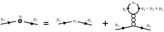
Figure 4: Dressed vertex associated to the bilocal currents

2.1 Dressing the bilocal vertex and other contributions in the NJL model

In addition to the contribution Eq. (15), in the NJL model we must consider also the dressing of the bilocal vertex due to the chiral interaction. This corresponds to change the bare vertex given in Table 1 by the dressed one depicted in Fig. 4. Therefore, instead of using $\bar{\Gamma}_{a_{1}}\,\delta\left(P^{+}x_{1}-\frac{1}{2}\left(p_{1}+p_{2}\right)^{+}\right)$ for the bare vertex in the Feynman amplitude in Eq. (17), we must use the replacement

$$\bar{\Gamma}_{a_{1}}\,\delta\left(P^{+}x_{1}-\frac{1}{2}\left(p_{1}+p_{2}\right)^{+}\right)$$

$$\longrightarrow \bar{\Gamma}_{a_{1}}\,\delta\left(P^{+}x_{1}-\frac{1}{2}\left(p_{1}+p_{2}\right)^{+}\right)$$

$$+\frac{2ig}{1-2g\,\Pi_{S}\left(q^{2}\right)}\left(-\right)\int\frac{d^{4}q_{1}}{\left(2\pi\right)^{4}}\delta\left(x_{1}P^{+}-q_{1}^{+}\right)\text{Tr}\left[iS_{F}\left(q_{1}\right)\,iS_{F}\left(q_{1}-q\right)\,\bar{\Gamma}_{a_{1}}\right]$$

$$+\sum_{j=1}^{3}i\gamma_{5}\tau^{j}\frac{2ig}{1-2g\,\Pi_{PS}\left(q^{2}\right)}\left(-\right)\int\frac{d^{4}q_{1}}{\left(2\pi\right)^{4}}\delta\left(x_{1}P^{+}-q_{1}^{+}\right)\text{Tr}\left[iS_{F}\left(q_{1}\right)\,i\gamma_{5}\tau^{j}\,iS_{F}\left(q_{1}-q\right)\,\bar{\Gamma}_{a_{1}}\right]\,,$$

where $q=p_{1}-p_{2}.$ Here, $\Pi_{S}$ and $\Pi_{PS}$ are the scalar and pseudo-scalar polarizations, respectively, defined in Appendix A.1.

Performing the explicit calculation of the dressing term, we found that it vanishes. Effectively, due to the fact that $q^{+}=0,$ the integrals over $q_{1}$ present in Eq. (LABEL:A.17) are

$$\int\frac{d^{4}q_{1}}{\left(2\pi\right)^{4}}\delta\left(x_{1}P^{+}-q_{1}^{+}\right)\,\text{Tr}\left[iS_{F}\left(q_{1}\right)\left(1,i\gamma_{5}\right)iS_{F}\left(q_{1}-q\right)\bar{\Gamma}_{a_{1}}\right] \propto$$

$$\int\frac{dq_{1}^{-}}{2\pi}\,\frac{f\left(q_{1},q\right)}{\left(2\,x_{1}P^{+}\right)^{2}\left(q_{1}^{-}-\frac{\vec{q}_{1\perp}^{2}+m^{2}}{2\,x_{1}P^{+}}+i\frac{\epsilon}{2\,x_{1}P^{+}}\right)\left(q_{1}^{-}-q^{-}-\frac{\left(\vec{q}_{1\perp}-\vec{q}_{\perp}\right)^{2}+m^{2}}{2\,x_{1}P^{+}}+i\frac{\epsilon}{2\,x_{1}P^{+}}\right)} =0\,\,,$$ (44)

being $f\left(q_{1},q\right)$ some function of $q^{-},$ $q_{\perp}$, $q_{1}^{-}$and $\vec{q}_{1\perp}.$ The last integral vanishes due to the fact that the poles of both propagators are in the same half complex plane. Therefore, the dressing of the bilocal vertex does not give any additional contribution to all the different pion dPDFs.

Two other types of possible contributions to the dPDFs, depicted in Fig 5, have to be considered. Despite the fact that, apparently, these two contributions are higher order contributions, chiral symmetry, present in the NJL model, ensures that they are of the same order than the one depicted in Fig. 1.

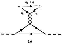
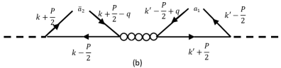
Figure 5: Other possible diagrams in the NJL model. All of them do not contribute to the dPDFs, as explained in the text.

The type of contribution shown in Fig. 5a represents the possibility that the two involved partons are originated by the same vacuum fluctuation, which, in order to make a connected diagram, has to be connected to the pion line. To analyze this kind of diagrams, we focus our attention on the upper triangle. In the particular case of the diagram of Fig. 5a we have, for this part,

$$\int\frac{d^{4}q_{1}}{\left(2\pi\right)^{4}}\delta\left(x_{2}P^{+}+q_{1}^{+}\right)\delta\left(x_{1}P^{+}-q_{1}^{+}\right)\,\text{Tr}\left[iS_{F}\left(q_{1}\right)\bar{\Gamma}_{a_{1}}iS_{F}\left(q_{1}+q\right)\bar{\Gamma}_{\bar{a}_{2}}iS_{F}\left(q_{1}\right)\right] \propto$$

$$\int\frac{dq_{1}^{-}}{2\pi}\,\frac{g\left(q_{1},q\right)}{\left(2\,x_{1}P^{+}\right)^{3}\left(q_{1}^{-}-\frac{\vec{q}_{1\perp}^{2}+m^{2}}{2\,x_{1}P^{+}}+i\frac{\epsilon}{2\,x_{1}P^{+}}\right)^{2}\left(q_{1}^{-}+q^{-}-\frac{\left(\vec{q}_{1\perp}+\vec{q}_{\perp}\right)^{2}+m^{2}}{2\,x_{1}P^{+}}+i\frac{\epsilon}{2\,x_{1}P^{+}}\right)} =0\,\,\,,$$ (45)

being $g\left(q_{1},q\right)$ some function of $q^{-},$ $q_{\perp}$, $q_{1}^{-}$ and $\vec{q}_{1\perp}.$ As in the case of Eq. (44), the last integral vanishes because all the poles of the propagators are in the same half complex plane. Therefore, diagrams of type of Fig. 5a give no contribution to the dPDFs. With respect to this, it is more interesting to see what happens with contributions of the type shown in Fig. 5b. Despite of their aspect, this kind of contributions are not related to the approximation to dPDF in terms of GPDs proposed in Refs. [7] and [8]. First of all, the intermediate state represented by the small bubbles has the quantum numbers of a pion. This part of the diagram gives a contribution which, close to the pion mass, can be approximated by the point-like pion propagator,

$$\frac{2ig_{0}}{1-2g_{0}\Pi_{PS}\left(\left(P-q\right)^{2}\right)}\simeq\frac{-i\,g_{\pi qq}^{2}}{\left(P-q\right)^{2}-m_{\pi}^{2}}\,.$$ (46)

According to Eq. (17), all possible diagrams have an overall $q^{-}$-integral. In the case of the present diagram, this integral only involves the pion propagator and two quark propagators, one from each of the triangles. Extracting these terms we obtain (here $h\left(k,\,k^{\prime},\,\vec{q}_{\perp},\,q^{-}\right)$ is some function of $q^{-},$ $q_{\perp}$, $k^{-},$ $\vec{k}_{\perp},$ $k^{\prime-},$ and $\vec{k}_{\perp}^{\prime}$)

$$\int\frac{dq^{-}}{2\pi}\frac{h\left(k,\,k^{\prime},\,\vec{q}_{\perp},\,q^{-}\right)}{\left[\left(P-q\right)^{2}-m_{\pi}^{2}+i\epsilon\right]\left[\left(k+\frac{P}{2}-q\right)^{2}-m^{2}+i\epsilon\right]\left[\left(k^{\prime}-\frac{P}{2}+q\right)^{2}-m_{\pi}^{2}+i\epsilon\right]}$$

$$=\frac{-1}{\left(2P^{+}\right)^{3}\,x_{1}\,x_{2}}$$ (47)

$$\left\{\frac{i\,\theta\left(-x_{1}\right)\,\theta\left(-x_{2}\right)\,h\left(k,\,k^{\prime},\,\vec{q}_{\perp},\,-\vec{q}_{\perp}^{2}/2P^{+}\right)}{\left[-\frac{\vec{q}_{\perp}^{2}}{2P^{+}}-k^{-}-\frac{P^{-}}{2}+\frac{\left(\vec{k}_{\perp}-\vec{q}_{\perp}\right)^{2}+m^{2}}{2P^{+}\,x_{1}}-\frac{i\epsilon\,\left(1-x_{1}\right)}{2P^{+}\,x_{1}}\right]\left[-\frac{\vec{q}_{\perp}^{2}}{2P^{+}}+k^{\prime-}-\frac{P^{-}}{2}+\frac{\left(\vec{k}_{\perp}^{\prime}+\vec{q}_{\perp}\right)^{2}+m^{2}}{2P^{+}\,x_{2}}-\frac{i\epsilon\left(1-x_{2}\right)}{2P^{+}\,x_{2}}\right]}\right.$$

$$-\frac{i\,\theta\left(-x_{1}\right)\,\theta\left(x_{2}\right)\,h\left(k,\,k^{\prime},\,\vec{q}_{\perp},\,k^{-}+\frac{P^{-}}{2}-\frac{\left(\vec{k}_{\perp}-\vec{q}_{\perp}\right)^{2}+m^{2}}{2P^{+}\,x_{1}}\right)}{\left[k^{-}+\frac{P^{-}}{2}-\frac{\left(\vec{k}_{\perp}-\vec{q}_{\perp}\right)^{2}+m^{2}}{2P^{+}\,x_{1}}\frac{\vec{q}_{\perp}^{2}}{2P^{+}}+\frac{i\epsilon\,\left(1-x_{1}\right)}{2P^{+}\,x_{1}}\right]\left[k^{-}+k^{\prime-}-\frac{\left(\vec{k}_{\perp}-\vec{q}_{\perp}\right)^{2}+m^{2}}{2P^{+}\,x_{1}}+\frac{\left(\vec{k}_{\perp}^{\prime}+\vec{q}_{\perp}\right)^{2}+m^{2}}{2P^{+}\,x_{2}}+\frac{i\epsilon\left(x_{2}-x_{1}\right)}{2P^{+}\,x_{1}\,x_{2}}\right]}$$

$$\left.-\frac{i\,\theta\left(x_{1}\right)\,\theta\left(-x_{2}\right)\,h\left(k,\,k^{\prime},\,\vec{q}_{\perp},\,k^{-}+\frac{P^{-}}{2}-\frac{\left(\vec{k}_{\perp}-\vec{q}_{\perp}\right)^{2}+m^{2}}{2P^{+}\,x_{1}}\right)}{\left[k^{-}+k^{\prime-}-\frac{\left(\vec{k}_{\perp}-\vec{q}_{\perp}\right)^{2}+m^{2}}{2P^{+}\,x_{1}}+\frac{\left(\vec{k}_{\perp}^{\prime}+\vec{q}_{\perp}\right)^{2}+m^{2}}{2P^{+}\,x_{2}}+\frac{i\epsilon\left(x_{2}-x_{1}\right)}{2P^{+}\,x_{1}\,x_{2}}\right]\left[k^{\prime-}-\frac{P^{-}}{2}+\frac{\left(\vec{k}_{\perp}^{\prime}+\vec{q}_{\perp}\right)^{2}+m^{2}}{2P^{+}\,x_{2}}-\frac{\vec{q}_{\perp}^{2}}{2P^{+}}-\frac{i\epsilon\left(1-x_{2}\right)}{2P^{+}\,x_{2}}\right]}\right\}\,.$$

The first line of this expression corresponds to the pion pole contribution and, therefore, it is the one that could be described by a ”two GPD” contribution. Actually, the fact that both $x_{1,2}$ are negative prevents us from this simple interpretation. In fact, what happens is that one of the remaining integrals, the one over $k^{-}$ or that over $k^{\prime-},$ vanishes, because all poles are in the same half complex plane. In the other two contributions present in Eq. (47), at least one of the $x_{1,2}$ is negative. In both cases one of the remaining integrals over $k^{-}$ or $k^{\prime-}$ vanishes by the same reasons than in the first case.

We want to emphasize that the vanishing of all diagrams of the type of Fig. 5 as well as the diagram related to the dressing of the non local vertex, depicted in Fig. 4 take place for all the different dPDFs. From a physical point of view, the position of the pole in the lower or the upper half complex plane corresponds to the two temporal contributions or, in other words, the position of the pole tells us if we are dealing with a particle or an antiparticle. The vanishing of all these integrals is related to the fact that we can not close a loop with only particles or only antiparticles. In all these diagrams, the fact that $q^{+}=0$, which prevents the presence of a particle and an antiparticle in the same non local vertex, guarantees that they do not give any additional contribution.

3 Test of factorization: an approximation to dPDFs in terms of GPDs

Since dPDFs are experimentally basically unknown, their size and properties are often inferred in terms of one-body quantities. In Refs. [7] and [8] it has been shown that, in a mean field approach, neglecting correlations between the involved partons, the dPDF $F_{q\bar{q}}$ in momentum space factorizes in the product of two GPDs at zero skewness. The validity of this factorization has been analyzed in a number of model calculations where it has been found to fail in general, in particular in the valence region at the momentum scale associated to the model [12, 13, 14, 15, 16, 17, 18, 24]. Let us now check whether or not the factorization in two GPDs, in the vector sector where it makes sense for a pion,

$$F_{u\bar{d}}^{\left(2GPD\right)}\left(x_{1},x_{2},\vec{q}_{\perp}\right)=H_{\pi^{+}}^{u}\left(x_{1},0,t\right)\,H_{\pi^{+}}^{d}\left(-x_{2},0,t\right)\,,$$ (48)

with $t=-\vec{q}_{\perp}^{\,2}$, is a good approximation to the full result of the present NJL approach, given by Eq. (22).

To illustrate this property practically, we evaluate integrals over the longitudinal variable $x_{2}$ for both quantities, the dPDF Eq. (22)

$$\bar{F}_{u\bar{d}}^{\left(0\right)}\left(x_{1},\vec{q}_{\perp}\right)=\int dx_{2}\,F_{u\bar{d}}^{\left(0\right)}\left(x_{1},x_{2},\vec{q}_{\perp}\right)$$ (49)

and the expression Eq. (48) :

$$\bar{F}_{u\bar{d}}^{\left(2GPD\right)}\left(x_{1},\vec{q}_{\perp}\right)=\int dx_{2}\,F_{u\bar{d}}^{\left(2GPD\right)}\left(x_{1},x_{2},\vec{q}_{\perp}\right)=H_{\pi^{+}}^{u}\left(x_{1},0,t\right)F_{\pi^{+}}(t)\,,$$ (50)

where, in the last line, use has been made of well known sum rules for GPDs, with $F_{\pi^{+}}(t)$ the pion electromagnetic form factor.

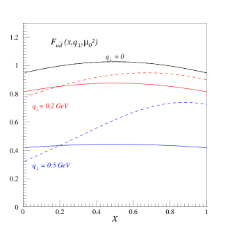
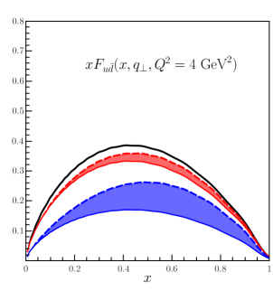
Figure 6: Comparison between Eq. (49) (full) and its approximation Eq. (50) (dashed). Left panel: results at the hadronic scale, $\mu_{o}$ = 0.29 GeV, for $q_{\perp}=0,0.2,0.5$ GeV. Right panel: the same as in the previous panel, but after LO QCD evolution to the momentum scale $Q^{2}$= 4 GeV² and multiplied, for an easy presentation, by the longitudinal momentum variable $x$. The quality of the approximation decreases as $q_{\perp}$ increases as emphasized by the shaded areas, showing the difference between the exact calculation and the approximation.

The comparison between Eqs. (49) and (50) is shown in the left panel of Fig. 6, using results of ref. [27] for the NJL GPD, for three low values of $q_{\perp}$, i.e., 0, 0.2 and 0.5 GeV. It is clear that the approximation in terms of two GPDs holds exactly at $q_{\perp}=0$, while it does not work at higher values of $q_{\perp}$, in the present NJL framework, in the valence sector. A similar conclusion was indeed obtained for the nucleon in Refs. [12, 13, 14, 15, 16, 17, 18], using low energy models, and recently, for the pion, using a light-front approach, in Ref. [24].

As already stated in the first section, the parton distribution obtained within a model should be associated to a low momentum scale, the so-called hadronic scale $\mu_{0}^{2}$. For the pion in the NJL model such a value can be fixed in $\mu_{0}=$ 0.29 GeV (see, e.g. Ref. [31]). Since the approximation Eq. (48) has been proposed for possible experimental observables measured at colliders, such as the LHC, at high momentum scales and typically at low values of the longitudinal momentum fractions $x_{1}$ and $x_{2}$, it is important to check whether the approximation works better at high $Q^{2}$ values. We have therefore performed the leading order QCD evolution of our results, from the scale $\mu_{0}^{2}$ to $Q^{2}=4$ GeV², following the evolution procedure described in Ref. [24]. The result is shown in the right panel of Fig. 6. It is clear that the difference between Eqs. (49) and (50) persists in the present NJL scenario, at least in the valence sector, even at high momentum scales, as found in Ref. [24] with a different dynamical input. Our model calculation shows that relevant novel information on two-body parton correlations, that are not included in one body quantities nor described in a mean field approach, would be accessible through experimental or lattice measurements of dPDFs.

4 Conclusions

A consistent field-theoretical approach, based on the Nambu–Jona-Lasinio model, with two different regulariztion schemes, the standard Pauli-Villars method and a properly introduced Light-Front one, is used for a systematic analysis of double parton distribution functions in the pion. Results are presented for several double parton distributions corresponding to different Dirac operators in their definitions. In particular, in the vector sector, it is found that these functions encode novel non-perturbative information, not present in one-body quantities, such as PDFs and GPDs, as it happens in model calculations of proton dPDFs as well as in the only phenomenological evaluation of pion dPDFs available at present. In particular, we have shown that the approximation of the momentum space spin-independent dPDF in terms of two GPDs at zero skewness does not hold in our approach. This fact is true also after QCD evolution of the model results, the latter being associated to a low hadronic scale, to experimental high momentum scales.

Lattice data have been already obtained for two current correlations in the pion, quantities related to dPDFs. The analysis of two curent correlations in the pion in the NJL would correspond to a completely different calculation, presently in progress [41], with respect to the one presented here. The evaluation of pion dPDFs on the lattice has been planned [42]. It will be interesting to compare our results for the physical dPDFs with the forth-coming lattice data.

Appendix A The NJL model and regularization scheme

A.1 Basic physical quantities in the NJL model

The Lagrangian density in the two-flavor version of the NJL model is [25]

$$\mathcal{L}=\bar{\psi}\left(i\,\not\partial-m_{0}\right)\psi+g\left[\left(\bar{\psi}\,\psi\right)^{2}+\left(\bar{\psi}\,\vec{\tau}\,i\gamma_{5}\,\psi\right)^{2}\right]\,\,,$$ (51)

where $m_{0}$ is the current quark mass. The NJL is a chiral theory that reproduces the spontaneous symmetry breaking process in which the quark mass moves from the current value to its constituent value,

$$m=m_{0}-4g\,\left\langle\bar{u}u\right\rangle\,,$$ (52)

where $\left\langle\bar{u}u\right\rangle$ is the quark condensate.

The main physical quantities associated to pion physics are defined in terms of two integrals:

$$I_{1}\left(m\right)=i\int\frac{d^{4}k}{\left(2\pi\right)^{4}}\frac{1}{k^{2}-m^{2}+i\epsilon}$$ (53)

$$I_{2}\left(m,q^{2}\right)=i\int\frac{d^{4}k}{\left(2\pi\right)^{4}}\frac{1}{\left[\left(k+\frac{q}{2}\right)^{2}-m^{2}+i\epsilon\right]\left[\left(k-\frac{q}{2}\right)^{2}-m^{2}+i\epsilon\right]}$$ (54)

Effectively, in the large $N_{c}$ approximation, the quark condensate is defined by

$$\left\langle\bar{u}u\right\rangle=-4N_{c}mI_{1}\,.$$ (55)

Pion and sigma masses are defined by the relations

$$2g\,\Pi_{PS}\left(m_{\pi}^{2}\right)=1\,\,\,\,\,\,\,\,\,,\,\,\,\,\,\,\,\,\,\,\,\,\,2g\,\Pi_{S}\left(m_{\sigma}^{2}\right)=1\,,$$ (56)

with the scalar polarization

$$\Pi_{S}\left(q^{2}\right) =-i\int\frac{d^{4}k}{\left(2\pi\right)^{4}}\text{Tr}\left[iS_{F}\left(p\right)\,iS_{F}\left(p-q\right)\right]$$

$$=8N_{c}\left[I_{1}+\frac{1}{2}\left(4m^{2}-q^{2}\right)I_{2}\left(q\right)\right]\,,$$ (57)

and the pseudoscalar polarization

$$\Pi_{PS}\left(q^{2}\right) =-i\int\frac{d^{4}k}{\left(2\pi\right)^{4}}\text{Tr}\left[i\gamma_{5}\tau^{i}\,iS_{F}\left(p\right)i\gamma_{5}\tau^{i}\,iS_{F}\left(p-q\right)\right]$$

$$=8N_{c}\left[I_{1}-\frac{1}{2}q^{2}I_{2}\left(q\right)\right]\,.$$ (58)

The pion-quark and sigma-quark coupling constant are respectively defined by

$$g_{\pi qq}^{2} =\left(\frac{\partial\Pi_{PS}\left(q^{2}\right)}{\partial q^{2}}\right)_{q^{2}=m_{\pi}^{2}}^{-1}=\frac{-1}{4N_{c}\left[I_{2}\left(m_{\pi}^{2}\right)+m_{\pi}^{2}\left(\partial I_{2}/\partial q^{2}\right)_{q^{2}=m_{\pi}^{2}}\right]}\,,$$

$$g_{\sigma qq}^{2} =\left(\frac{\partial\Pi_{S}\left(q^{2}\right)}{\partial q^{2}}\right)_{q^{2}=m_{\sigma}^{2}}^{-1}=\frac{-1}{4N_{c}\left[I_{2}\left(m_{\sigma}^{2}\right)-\left(4m^{2}-m_{\sigma}^{2}\right)\left(\partial I_{2}/\partial q^{2}\right)_{q^{2}=m_{\sigma}^{2}}\right]}\,.$$

The pion decay constant are

$$f_{\pi}=-4N_{c}g_{\pi qq}mI_{2}\left(m_{\pi}^{2}\right)\,,$$ (60)

The NJL model is a non-renormalizable field theory and a regularization procedure has to be defined for the calculation of $I_{1}\left(m\right)$ and $I_{2}\left(m,q^{2}\right).$ We will introduce now the Pauli-Villars regularization method for the NJL model and, in section A.3, we built a regularization method adapted for calculations in the Light Front formalism.

A.2 Pauli Villars regularization scheme

In Section 2, we have used the Pauli-Villars regularization in order to render the occurring integrals finite. The way to proceed in this method is: (1) remove from the numerator all the powers of the integrated momentum, which will be replaced by external momenta, and the mass of the constituent quark, $m$; (2) for each resulting integral, which is of the form

$$\widetilde{I}_{n}\left(\mu\left(m\right)\right)=\int\frac{d^{4}k}{\left(2\pi\right)^{4}}\frac{1}{\left[k^{2}-\mu\left(m\right)^{2}+i\epsilon\right]^{n}}\,,$$ (61)

make the substitution

$$\widetilde{I}_{n}^{r}\left(\mu\left(m\right)\right)=\sum_{j=0}^{2}\,c_{j}\,\widetilde{I}_{n}\left(\mu\left(M_{j}\right)\right)\,,$$ (62)

with $M_{j}^{2}=m^{2}+j\,\Lambda^{2}$, $c_{0}=c_{2}=1$ and $c_{1}=-2$.

Following this procedure, we obtain for the momentum integral of one propagator

$$I_{1}=\frac{1}{16\pi^{2}}\sum_{j=0}^{2}c_{j}M_{j}^{2}\ln\frac{M_{j}^{2}}{m^{2}}\,,$$ (63)

and for the one of two propagators

$$I_{2}\left(m,q^{2}\right) =\frac{1}{16\pi^{2}}\sum_{j=0}^{2}c_{j}\left(\ln\frac{M_{j}^{2}}{m^{2}}+2\sqrt{\frac{4M_{j}^{2}}{q^{2}}-1}\,\arctan\frac{1}{\sqrt{\frac{4M_{j}^{2}}{q^{2}}-1}}\right)\,.$$ (64)

With the conventional values $\left\langle\bar{u}u\right\rangle=-(0.250\,\text{GeV})^{3},$ $f_{\pi}=0.0924\,\text{GeV}$ and $m_{\pi}=0.140\,\text{GeV}$, we get $m=0.238\,\text{GeV}$, $\Lambda$=0.860 GeV and $m_{0}=5.4\,\text{MeV}.$ For the pion-quark coupling constant we get $g_{\pi qq}^{2}=6.279.$ We can obtain the chiral limit taking $m_{0}=0$, without changing $\Lambda$ and $m.$ In that case $\left\langle\bar{u}u\right\rangle$ and $f_{\pi}$ do not change but one has $m_{\pi}=0$ and $g_{\pi qq}^{2}=6.625.$

A.3 A regularization of the NJL model in the Light Front

The Pauli-Villars (PV) regularization scheme, which respects the gauge symmetry of the problem, has been often adopted. Nevertheless, this procedure is based on an equal time quantization of the field theory, while the dPDF are defined in the light front formalism. In many cases this point has no consequences, but sometimes it does, as we will see later. Other usual regularization schemes, like the covariant four-momentum cutoff, the three momentum cutoff or the proper time regularization, are also defined in the equal time quantization of the field theory and they are manifestly not useful in a light front calculation.

Our aim, in this section, is to define a regularization procedure for the NJL model which respects the light front formalism. The ideal scheme will be: (1) to integrate $k^{-}$ using the poles of the propagators and, as a result of this integration, the range of variation of $k^{+}$ will be bounded; (2) introducing a cut-off,$\left|\vec{k}_{\perp}\right|<\Lambda_{\perp}$, to perform the integration over $\vec{k}_{\perp}$ and the integration over the bounded range of variation of $k^{+}$.

To have a clear notation, we call $\tilde{m}_{0}$ and $\tilde{m}$ the current and constituent quark masses evaluated in this aproach. The gap equation,

$$\tilde{m}=\tilde{m}_{0}-4g\,\left\langle\bar{u}u\right\rangle\,,$$ (65)

will be always valid.

The defined procedure works for $I_{2}\left(\tilde{m},q^{2}\right).$ Effectively, after integration over $k^{-}$ and introducing the change of variable $k^{+}=\left(x-\frac{1}{2}\right)\left|q^{+}\right|$, we have from Eq. (54) (for simplicity we can choose $q^{\mu}=\left(q^{+},\vec{0}_{\perp},q^{-}\right)$ and $q^{2}=2\,q^{+}q^{-}),$

$$I_{2}\left(\tilde{m},q^{2}\right)=-\frac{1}{16\,\pi^{2}}\int_{0}^{1}\,dx\,\int_{0}^{\Lambda_{\perp}^{2}}\,dk_{\perp}^{2}\,\frac{1}{k_{\perp}^{2}+\tilde{m}^{2}-q^{2}x\left(1-x)\right)}\,,$$ (66)

and, performing these two integrations we arrive to

$$I_{2}\left(\tilde{m},q^{2}\right)=\frac{1}{16\,\pi^{2}}\left[\ln\frac{\tilde{m}^{2}}{\Lambda_{\perp}^{2}+\tilde{m}^{2}}+\phi\left(\frac{q^{2}}{\tilde{m}^{2}}\right)-\phi\left(\frac{q^{2}}{\Lambda_{\perp}^{2}+\tilde{m}^{2}}\right)\right]\quad,$$ (67)

with

$$\phi\left(z\right)=\begin{cases}\sqrt{1-4/z}\,\ln\frac{\sqrt{1-4/z}+1}{\sqrt{1-4/z}-1}\,,&z<0\\ \\ 2\sqrt{\frac{4}{z}-1}\arctan\frac{1}{\sqrt{\frac{4}{z}-1}}\,,&0<z<4\\ \\ \sqrt{1-4/z}\,\left(\ln\frac{1+\sqrt{1-4/z}}{1-\sqrt{1-4/z}}-i\pi\right)\,,&4<z\quad.\end{cases}$$ (68)

The procedure that has allowed us to evaluate $I_{2}\left(\tilde{m},q^{2}\right)$ is not sufficient to determine $I_{1}\left(\tilde{m}\right).$ In fact, this is a well known problem: $I_{1}\left(\tilde{m}\right)$ corresponds to a tadpole diagram associated to the vacuum condensate, which is evaluable in a regularization scheme in an equal time formulation of the quantum field theory (like PV regulaization), but needs for additional assumptions in order to be evaluated in a light front formulation [43, 44].

Nevertheless, some information on $I_{1}\left({m}\right)$ can be obtained from $I_{2}\left({m},q^{2}\right)$, using the fact that

$$\frac{d}{d\tilde{m}^{2}}I_{1}\left(\tilde{m}\right)=\lim_{q^{\mu}\rightarrow 0}\,I_{2}\left(\tilde{m},q^{2}\right)\,.$$ (69)

From our result Eq. (67) we have

$$I_{1}\left(\tilde{m}\right)=\frac{1}{16\,\pi^{2}}\left[C\left(\Lambda_{\perp}\right)-\left(\Lambda_{\perp}^{2}+\tilde{m}^{2}\right)\ln\frac{\Lambda_{\perp}^{2}+\tilde{m}^{2}}{\Lambda_{\perp}^{2}}+\tilde{m}^{2}\ln\frac{\tilde{m}^{2}}{\Lambda_{\perp}^{2}}\right]\,,$$ (70)

where $C\left(\Lambda_{\perp}\right)$ is an arbitrary function of $\Lambda_{\perp}.$ Therefore, Eq. (69) fixes the dependence of $I_{1}\left(\tilde{m}\right)$ on $\tilde{m}$, but we need some additional input to fix its dependence on $\Lambda_{\perp}.$

We can perform explicitly the $k^{-}$ integral present in $I_{1}\left(\tilde{m}\right)$ obtaining

$$I_{1}\left(\tilde{m}\right)=\int\frac{d^{2}k_{\perp}}{16\,\pi^{3}}\int_{0}^{\infty}\frac{dk^{+}}{k^{+}}\,.$$ (71)

Now, for the $k^{+}$ integral we introduce an infrared and an ultraviolet cut-off imposing [45]

$$\frac{k_{\perp}^{2}+\tilde{m}^{2}}{\Lambda^{+}}<k^{+}<\Lambda^{+}\,,$$ (72)

and we arrive to

$$I_{1}\left(\tilde{m}\right) = \int_{0}^{\Lambda_{\perp}^{2}}\frac{dk_{\perp}^{2}}{16\,\pi^{2}}\ln\frac{2\Lambda^{+2}}{k_{\perp}^{2}+\tilde{m}^{2}}$$ (73)

$$= \frac{1}{16\,\pi^{2}}\left[\Lambda_{\perp}^{2}\left(1+\ln\frac{2\,\Lambda^{+2}}{\Lambda_{\perp}^{2}}\right)-\left(\Lambda_{\perp}^{2}+\tilde{m}^{2}\right)\ln\frac{\Lambda_{\perp}^{2}+\tilde{m}^{2}}{\Lambda_{\perp}^{2}}+\tilde{m}^{2}\ln\frac{\tilde{m}^{2}}{\Lambda_{\perp}^{2}}\right]\,.$$

This result is consistent with Eq. (70) and, in agreement with the discussion in Ref. [43, 44], we need an additional information because we have two different cutoffs. On the mass shell we have that $k^{+}=\frac{1}{\sqrt{2}}\left(E+k^{3}\right)$ and, assuming that $k^{3}<\Lambda_{\perp},$ a natural way to relate both cutoffs is to use $\Lambda^{+}=\sqrt{2}\Lambda_{\perp}.$ In this way, we finally obtain

$$I_{1}\left(\tilde{m}\right)=\frac{1}{16\,\pi^{2}}\left[\Lambda_{\perp}^{2}\left(1+\ln 4\right)-\left(\Lambda_{\perp}^{2}+\tilde{m}^{2}\right)\ln\frac{\Lambda_{\perp}^{2}+\tilde{m}^{2}}{\Lambda_{\perp}^{2}}+\tilde{m}^{2}\ln\frac{\tilde{m}^{2}}{\Lambda_{\perp}^{2}}\right]\,.$$ (74)

As explained in Ref. [45], the choice made in Eq. (72) for the cutoffs, relating the ultraviolet and the infrared ones, is natural on the basis of the respect of the dispersion relation $2k^{+}k^{-}-k_{\perp}^{2}=\tilde{m}^{2}$ and on the restoration of the symmetry between $k^{+}$ and $k^{-}.$ Parity transformation implies the exchange of $k^{+}$ and $k^{-},$ therefore the minimum value of $k^{+}$ must be related to the maximum value of $k^{-}$ through the dispersion relation and the assumption of the same maximum value for $k^{+}$ and $k^{-}.$

In this scheme, with the conventional values $\left\langle\bar{u}u\right\rangle=-(0.250\,\text{GeV})^{3},$ $f_{\pi}=0.0924\,\text{GeV}$ and $m_{\pi}=0.140\,\text{GeV}$, we get $\tilde{m}=0.246\,\text{GeV}$, $\Lambda_{\perp}$=0.572 GeV and $\tilde{m}_{0}=5.3\,\text{MeV}.$ For the pion-quark coupling constant we get $\tilde{g}_{\pi qq}^{2}=6.735.$ We can obtain the chiral limit taking $\tilde{m}_{0}=0$, without changing $\Lambda_{\perp}$ and $\tilde{m}.$ In that case $\left\langle\bar{u}u\right\rangle$ and $f_{\pi}$ do not change but one has $m_{\pi}=0$ and $\tilde{g}_{\pi qq}^{2}=7.085\,.$

A.4 Some intermediate results

The traces involved in Eq. (19) are:

$$\begin{array}[]{lll}tr_{u,\bar{d}}\left(\vec{k}_{\perp},\,\vec{q}_{\perp}\right)&=&-2\,P^{+2}\,\left[\vec{k}_{\perp}^{\thinspace 2}-\frac{1}{4}\vec{q}_{\perp}^{\thinspace 2}+m^{2}\right]\\ tr_{\Delta u,\Delta\bar{d}}\left(\vec{k}_{\perp},\,\vec{q}_{\perp}\right)&=&-2\,P^{+2}\,\left[\vec{k}_{\perp}^{\thinspace 2}-\frac{1}{4}\vec{q}_{\perp}^{\thinspace 2}-m^{2}\right]\\ tr_{\delta u^{j},\delta\bar{d}^{k}}\left(\vec{k}_{\perp},\,\vec{q}_{\perp}\right)&=&2\,P^{+2}\,\left[-2\,k_{\perp}^{j}\,k_{\perp}^{k}+\frac{1}{2}\,q_{\perp}^{j}\,q_{\perp}^{k}+\delta^{j,k}\,\left(\vec{k}_{\perp}^{\thinspace 2}-\frac{1}{4}\vec{q}_{\perp}^{\thinspace 2}+m^{2}\right)\right]\\ tr_{S,S}\left(\vec{k}_{\perp},\,\vec{q}_{\perp}\right)&=&\frac{1}{2}m_{\pi}^{2}\,\left(4\,m^{2}+\vec{q}_{\perp}^{\thinspace 2}\right)\\ tr_{P,P}\left(\vec{k}_{\perp},\,\vec{q}_{\perp}\right)&=&\frac{1}{2}m_{\pi}^{2}\,\vec{q}_{\perp}^{\thinspace 2}\end{array}$$ (75)

$$\begin{array}[]{llccl}tr_{u,\Delta\bar{d}}\left(\vec{k}_{\perp},\,\vec{q}_{\perp}\right)&=&tr_{\Delta u,\bar{d}}\left(\vec{t}_{\perp},\,\vec{q}_{\perp},y\right)&=&-2\,i\,P^{+2}\,\epsilon^{j,k}\,k_{\perp}^{j}\,q_{\perp}^{k}\\ tr_{u,\delta\bar{d}^{j}}\left(\vec{k}_{\perp},\,\vec{q}_{\perp}\right)&=&-tr_{\delta u^{j},\bar{d}}\left(\vec{t}_{\perp},\,\vec{q}_{\perp}\right)&=&2\,i\,P^{+2}\,m\,\epsilon^{j,k}\,q_{\perp}^{k}\\ tr_{\Delta u,\delta\bar{d}^{j}}\left(\vec{k}_{\perp},\,\vec{q}_{\perp}\right)&=&-tr_{\delta u^{j},\Delta\bar{d}}\left(\vec{t}_{\perp},\,\vec{q}_{\perp}\right)&=&4\,m\,P^{+2}\,k_{\perp}^{j}\end{array}$$ (76)

with $\epsilon^{j,k}=\epsilon^{0,j,k,3}.$

Using the relation

$$\int\frac{d^{2}k_{\perp}}{\left(2\pi\right)^{2}} \frac{k_{\perp}^{j}\,k_{\perp}^{k}}{\left[\left(\vec{k}_{\perp}+\frac{q_{\perp}}{2}\right)^{2}+m^{2}-x_{1}\left(1-x_{1}\right)m_{\pi}^{2}-i\epsilon\right]\left[\left(\vec{k}_{\perp}-\frac{q_{\perp}}{2}\right)^{2}+m^{2}-x_{1}\left(1-x_{1}\right)m_{\pi}^{2}-i\epsilon\right]}=$$

$$\int\frac{d^{2}k_{\perp}}{\left(2\pi\right)^{2}} \frac{\left[\delta^{jk}\left(k_{\perp}^{2}-\frac{1}{q_{\perp}^{2}}\left(\vec{k}_{\perp}\cdot\vec{q}_{\perp}\right)^{2}\right)+\hat{q}_{\perp}^{j}\,\hat{q}_{\perp}^{k}\left(\frac{2}{q_{\perp}^{2}}\left(\vec{k}_{\perp}\cdot\vec{q}_{\perp}\right)^{2}-k_{\perp}^{2}\right)\right]}{\left[\left(\vec{k}_{\perp}+\frac{q_{\perp}}{2}\right)^{2}+m^{2}-x_{1}\left(1-x_{1}\right)m_{\pi}^{2}-i\epsilon\right]\left[\left(\vec{k}_{\perp}-\frac{q_{\perp}}{2}\right)^{2}+m^{2}-x_{1}\left(1-x_{1}\right)m_{\pi}^{2}-i\epsilon\right]}\,$$ (77)

we observe that the tensor trace can be rewritten as

$$tr_{\delta u^{j},\delta\bar{d}^{k}}\left(\vec{k}_{\perp},\,\vec{q}_{\perp}\right)=2\,P^{+2}\,\left[\left(2\,\hat{q}_{\perp}^{j}\,\hat{q}_{\perp}^{k}-\delta^{j,k}\right)\left(k_{\perp}^{\thinspace 2}+\frac{q_{\perp}^{\thinspace 2}}{4}-\frac{2}{q_{\perp}^{2}}\left(\vec{k}_{\perp}\cdot\vec{q}_{\perp}\right)^{2}\right)+\delta^{j,k}\,m^{2}\right]\,,$$ (78)

showing in an explicit form the tensor structure defined in Eq. (9) for $F_{\delta q^{j},\delta\bar{q}^{k}}\left(x_{1},x_{2},\vec{q}_{\perp}^{\,2}\right).$

All these traces are of the generic form

$$tr_{a_{1}\bar{a}_{2}}\left(\vec{k}_{\perp},\,\vec{q}_{\perp}\right)=2\,P^{+2}\,\left[A\,k_{\perp}^{2}+\vec{B}\cdot\vec{k}_{\perp}+D+G\left(\vec{q}_{\perp}\cdot\vec{k}_{\perp}\right)^{2}\right]\,,$$ (79)

where $A,\,\vec{B},\,D$ and $G$ are functions of $\vec{q}_{\perp}$ and $m$ but $\vec{k}_{\perp}$-independent. The linear terms in $\vec{k}_{\perp}$ in Eq. (79) will vanish after the $\vec{k}_{\perp}$ integration present in Eq. (18). Therefore, the final result can be written as (we follow here the notation used in Eqs. (22-28)),

$$F_{a_{1},\bar{a_{2}}}\left(x_{1},x_{2},\vec{q}_{\perp}\right)=-C\left(x_{1},x_{2}\right)\left[A\,I_{A}^{r}+\frac{D}{q_{\perp}^{2}}\,I_{D}^{r}+G\,q_{\perp}^{2}\,I_{G}^{r}\right]\,.$$ (80)

In order to obtain Eq (22-28) in the Pauli-Villars regularization scheme from Eq. (18) we join the two propagators using Feynman parametrization, we make the change of variable $\vec{k}_{\perp}=\vec{t}_{\perp}-\vec{q}_{\perp}\left(y-1/2\right)$ and we remove the $t_{\perp}^{2}$ present in the numerator before integration. For instance, in the case of $I_{A}^{r}$ we have, before the regularization,

$$I_{A} =4\pi\,\int\frac{d^{2}k_{\perp}}{\left(2\pi\right)^{2}}$$

$$\frac{k_{\perp}^{2}}{\left[\left(\vec{k}_{\perp}+\frac{q_{\perp}}{2}\right)^{2}+m^{2}-x_{1}\left(1-x_{1}\right)m_{\pi}^{2}-i\epsilon\right]\left[\left(\vec{k}_{\perp}-\frac{q_{\perp}}{2}\right)^{2}+m^{2}-x_{1}\left(1-x_{1}\right)m_{\pi}^{2}-i\epsilon\right]}$$

$$=4\pi\,\left[\int_{0}^{1}\,dy\,\int\frac{d^{2}t_{\perp}}{\left(2\pi\right)^{2}}\frac{1}{\left[t_{\perp}^{2}+q_{\perp}^{2}y\left(1-y\right)+\kappa-i\epsilon\right]}\right.$$

$$-2q_{\perp}^{2}\,\int_{0}^{1}\,dy\,\int\frac{d^{2}t_{\perp}}{\left(2\pi\right)^{2}}\frac{y\left(1-y\right)}{\left[t_{\perp}^{2}+q_{\perp}^{2}y\left(1-y\right)+\kappa-i\epsilon\right]^{2}}$$

$$-\left.\left(\kappa-\frac{1}{4}q_{\perp}^{2}\right)\,\int_{0}^{1}\,dy\,\int\frac{d^{2}t_{\perp}}{\left(2\pi\right)^{2}}\frac{1}{\left[t_{\perp}^{2}+q_{\perp}^{2}y\left(1-y\right)+\kappa-i\epsilon\right]^{2}}\right]\,.$$ (81)

Now we perform each integral using standard methods and we regularize it, obtaining

$$I_{A}^{r\left(PV\right)}=\sum_{i=0}^{2}\,c_{i}\,\left(-\ln\frac{\kappa_{i}}{\kappa}-\left(2\frac{\kappa}{q_{\perp}^{2}}+\frac{1}{2}\right)f\left(\frac{\kappa_{i}}{q_{\perp}^{2}}\right)\right)\,.$$ (82)

Following the same procedure we have

$$I_{D}^{r\left(PV\right)} =\sum_{i=0}^{2}\,c_{i}\,f\left(\frac{\kappa_{i}}{q_{\perp}^{2}}\right)\,,$$ (83)

$$I_{G}^{r\left(PV\right)} =\sum_{i=0}^{2}\,c_{i}\,\left(-\frac{1}{2}\ln\frac{\kappa_{i}}{\kappa}-\frac{m^{2}-M_{i}^{2}}{q_{\perp}^{2}}\,f\left(\frac{\kappa_{i}}{q_{\perp}^{2}}\right)\right)\,.$$

Eqs. (32-38) have been obtained in the LF regularization scheme. In this case we have, for the $I_{A}^{r}$ contribution,

$$I_{A}^{r\left(LF\right)}=4\pi\,\int_{0}^{\Lambda_{\perp}}\frac{dk_{\perp}}{\left(2\pi\right)^{2}}\,k_{\perp}\,\int_{0}^{2\pi}\,d\theta\,\frac{k_{\perp}^{2}}{\left(k_{\perp}^{2}+\frac{q_{\perp}^{2}}{4}+\tilde{\kappa}\right)^{2}-k_{\perp}^{2}\,q_{\perp}^{2}\,\cos^{2}\theta}\,.$$ (84)

Here, both integrals, on $\theta$ and on $k_{\perp},$ can be performed obtaining

$$I_{A}^{r\left(LF\right)}=g_{2}\left(q_{\perp}\right)\,,$$ (85)

and, in a similar way,

$$I_{D}^{r\left(LF\right)} =g_{0}\left(q_{\perp}\right)\,,$$ (86)

$$I_{G}^{r\left(LF\right)} =\tilde{g}_{2}\left(q_{\perp}\right)\,,$$

are obtained.

References

- [1] P. Bartalini and J. R. Gaunt, Adv. Ser. Direct. High Energy Phys. 29 (2018) pp.1. doi:10.1142/10646
- [2] G. Aad et al. [ATLAS Collaboration], New J. Phys. 15 (2013) 033038.
- [3] N. Paver and D. Treleani, Nuovo Cim. A 70 (1982) 215.
- [4] M. Diehl, D. Ostermeier and A. Schafer, JHEP 03, 089 (2012).
- [5] M. Guidal, H. Moutarde and M. Vanderhaeghen, Rept. Prog. Phys. 76 (2013) 066202.
- [6] R. Dupré, M. Guidal and M. Vanderhaeghen, Phys. Rev. D 95 (2017) no.1, 011501.
- [7] B. Blok, Y. Dokshitser, L. Frankfurt and M. Strikman, Eur. Phys. J. C 72, 1963 (2012).
- [8] B. Blok, Y. Dokshitzer, L. Frankfurt and M. Strikman, Eur. Phys. J. C 74, 2926 (2014).
- [9] A. Del Fabbro and D. Treleani, Phys. Rev. D 63, 057901 (2001).
- [10] M. Rinaldi and F. A. Ceccopieri, Phys. Rev. D 97, no. 7, 071501 (2018); M. Rinaldi and F. A. Ceccopieri, JHEP 1909 (2019) 097.
- [11] T. Kasemets and S. Scopetta, Adv. Ser. Direct. High Energy Phys. 29 (2018) 49 doi:10.1142/9789813227767_0004 [arXiv:1712.02884 [hep-ph]].
- [12] H. M. Chang, A. V. Manohar and W. J. Waalewijn, Phys. Rev. D 87 (2013) no.3, 034009.
- [13] M. Rinaldi, S. Scopetta and V. Vento, Phys. Rev. D 87, 114021 (2013).
- [14] M. Rinaldi, S. Scopetta, M. Traini and V. Vento, JHEP 12, 028 (2014).
- [15] T. Kasemets and A. Mukherjee, Phys. Rev. D 94, no. 7, 074029 (2016).
- [16] M. Rinaldi, S. Scopetta, M. Traini and V. Vento, Phys. Lett. B 752, 40 (2016).
- [17] M. Rinaldi, S. Scopetta, M. C. Traini and V. Vento, JHEP 16, 063 (2016).
- [18] M. Traini, M. Rinaldi, S. Scopetta and V. Vento, Phys. Lett. B 768 (2017) 270.
- [19] R. Kirschner, Phys. Lett. 84B (1979) 266.
- [20] V. P. Shelest, A. M. Snigirev and G. M. Zinovev, Phys. Lett. 113B (1982) 325.
- [21] M. Diehl and J. R. Gaunt, Adv. Ser. Direct. High Energy Phys. 29 (2018) 7 [arXiv:1710.04408 [hep-ph]].
- [22] C. Zimmermann [RQCD Collaboration], PoS LATTICE 2016, 152 (2016).
- [23] G. S. Bali et al., JHEP 1812 (2018) 061 doi:10.1007/JHEP12(2018)061 [arXiv:1807.03073 [hep-lat]].
- [24] M. Rinaldi, S. Scopetta, M. Traini and V. Vento, Eur. Phys. J. C 78 (2018) no.9, 781.
- [25] S. P. Klevansky, Rev. Mod. Phys. 64 (1992) 649.
- [26] R. M. Davidson and E. Ruiz Arriola, Acta Phys. Polon. B 33 (2002) 1791.
- [27] L. Theussl, S. Noguera and V. Vento, Eur. Phys. J. A 20 (2004) 483.
- [28] E. Ruiz Arriola and W. Broniowski, Phys. Rev. D 66 (2002) 094016.
- [29] A. Courtoy and S. Noguera, Phys. Lett. B 675 (2009) 38.
- [30] A. Courtoy and S. Noguera, Phys. Rev. D 76 (2007) 094026.
-
[31]
A. Courtoy, Ph. D. Thesis, Valencia University, 2009.
http://arxiv.org/abs/arXiv:1010.2974 - [32] S. Noguera and S. Scopetta, Phys. Rev. D 85 (2012) 054004.
- [33] H. Weigel, E. Ruiz Arriola and L. P. Gamberg, Nucl. Phys. B560 (1999) 383.
- [34] S. Noguera and S. Scopetta, JHEP 1511 (2015) 102.
- [35] W. Broniowski and E. Ruiz Arriola, Phys. Rev. D 97 (2018) no.3, 034031.
- [36] F. A. Ceccopieri, A. Courtoy, S. Noguera and S. Scopetta, Eur. Phys. J. C 78, no. 8, 644 (2018).
- [37] J. R. Gaunt and W. J. Stirling, JHEP 1003 (2010) 005.
- [38] A. V. Radyushkin, Phys. Rev. D 56 (1997) 5524.
- [39] X. D. Ji, J. Phys. G 24 (1998) 1181.
- [40] M. Diehl and T. Kasemets, JHEP 1305, 150 (2013) doi:10.1007/JHEP05(2013)150 [arXiv:1303.0842 [hep-ph]].
- [41] A. Courtoy, S. Noguera and S. Scopetta, in progress.
- [42] C. Zimmermann, private communication.
- [43] M. Burkardt, Adv. Nucl. Phys. 23 (1996) 1 [hep-ph/9505259].
- [44] M. Burkardt, In *Seoul 1997, QCD, lightcone physics and hadron phenomenology* 170-199 [hep-ph/9709421].
- [45] K. Itakura and S. Maedan, Phys. Rev. D 62, 105016 (2000).