Multi-level Bayes and MAP monotonicity testing

Abstract

In this paper, we develop Bayes and maximum a posteriori probability (MAP) approaches to monotonicity testing. In order to simplify this problem, we consider a simple white Gaussian noise model and with the help of the Haar transform we reduce it to the equivalent problem of testing positivity of the Haar coefficients. This approach permits, in particular, to understand links between monotonicity testing and sparse vectors detection, to construct new tests, and to prove their optimality without supplementary assumptions. The main idea in our construction of multi-level tests is based on some invariance properties of specific probability distributions. Along with Bayes and MAP tests, we construct also adaptive multi-level tests that are free from the prior information about the sizes of non-monotonicity segments of the function.

Keywords: Haar transform, Bayes and MAP tests, multi-level hypothesis testing, stable distributions, type I and II error probabilities, critical signal-noise ratio.

AMS Subject Classification 2010: Primary 62C20; secondary 62J05.

1 Introduction

The literature on non-parametric monotonicity testing deals usually with the model

$$Y=f(X)+\xi,$$

where $Y$ is a scalar dependent random variable, $X$ a scalar independent random variable, $f(\cdot)$ an unknown function, and $\xi$ an unobserved scalar random variable with $\mathbf{E}\{\xi|X\}=0$. We are interested in testing the null hypothesis, $\mathbf{H}_{0}$ that $f(x)$ is increasing against the alternative, $\mathbf{H}_{1}$ that there are $x_{1}$ and $x_{2}$ such that $x_{1}<x_{2}$ and $f(x_{1})>f(x_{2})$. The decision is to be made based on the i.i.d. sample $\{X_{i},Y_{i}\}_{1\leq i\leq n}$ from the distribution of $(X,Y)$. Typical applications of monotonicity testing are related to econometric models, see, e.g., Chetverikov [4].

Usual approaches to this problem have in their core simple heuristic ideas and assumptions. So, the tests proposed in Gijbels et. al. [9] and Ghosal, Sen, and van der Vaart [8] are based on the signs of $(Y_{i+k}-Y_{i})(X_{i+k}-X_{i})$. Hall and Heckman [10] developed a test based on the slopes of local linear estimates of $f(\cdot)$. Along with these papers we can cite Schlee [15], Bowman, Jones, and Gijbels [2], Dümbgen and Spokoiny [6], Durot [7], Baraud, Huet, and Laurent [1], Wang and Meyer [17], and Chetverikov [4]. As to typical hypothesis about $f(\cdot)$, it is often assumed that $f(x)$ is a Lipschitz function, i.e.,

$$|f(y)-f(x)|\leq L|y-x|,$$

where the constant $L<\infty$ may be known or unknown.

In this paper, we look at the problem of monotonicity testing from a little different and less intuitive viewpoint. As we will see below, our approach permits, in particular, to understand links between this problem and sparse vectors detection and to construct new powerful tests. In order to simplify technical details and to get rid of supplementary assumptions, we begin with monotonicity testing of an unknown function $f(t),\,t\in[0,1]$, in the so-called white noise model similar to that one considered in [6]. So, it is assumed we have at our disposal the noisy data

$$Y(t)=f(t)+\sigma n(t),\ t\in[0,1],$$ (1)

where $n(\cdot)$ is a standard white Gaussian noise and $\sigma>0$ is a known noise level. With the help of these observations we want to test

the null hypothesis

$${\bf H}_{0}:\ f^{\prime}(t)\geq 0,\,\text{for all}\ t\in[0,1],$$

vs. the alternative

$${\bf H}_{1}:\ f^{\prime}(t)<0,\,\text{for some}\ t\in[0,1].$$

Our approach to this problem is based on estimating the following linear functionals:

$$\theta_{h,t}(f)\stackrel{{\scriptstyle\rm def}}{{=}}\frac{1}{{h}}\int_{t}^{t+h}f(u)\,du-\frac{1}{{h}}\int_{t-h}^{t}f(u)\,du$$

for all $h,t$ that are admissible, i.e., such that $[t-h,t+h]\subseteq[0,1]$. It is clear that $\theta_{h,t}(f)/h$ may be interpreted as approximations of the derivative $f^{\prime}(t)$ since

$$\lim_{h\rightarrow 0}\frac{\theta_{h,t}(f)}{h}=f^{\prime}(t),$$

for any given $t\in(0,1)$.

With the help of (1), the functionals $\theta_{h,t}(f)$ are estimated as follows:

$$\hat{\theta}_{h,t}(Y)=\frac{1}{{h}}\int_{t}^{t+h}Y(u)\,du-\frac{1}{{h}}\int_{t-h}^{t}Y(u)\,du$$

and these estimates admit the obvious representation

$$\hat{\theta}_{h,t}(Y)={\theta}_{h,t}(f)+\sigma_{h}\xi_{h,t},$$ (2)

where

$$\sigma_{h}=\sigma\sqrt{\frac{2}{h}},\quad\xi_{h,t}=\frac{1}{{\sqrt{2h}}}\biggl{[}\int_{t}^{t+h}n(u)\,du-\int_{t-h}^{t}n(u)\,du\biggr{]}\sim\mathcal{N}(0,1).$$

Notice that if $\mathbf{H}_{0}$ is true, then $\theta_{h,t}(f)\geq 0$ for all admissible $h,t$, otherwise ($\mathbf{H}_{1}$ is true) there exist $h^{\prime},t^{\prime}$ such that $\theta_{h^{\prime},t^{\prime}}(f)<0$. That is why in what follows we will focus on testing

$$\begin{split}&\textsl{the null hypothesis}\\ &{\bf H}_{0}:\ \theta_{h,t}(f)\geq 0,\ \textit{for all admissible}\ h,t\\ &\textsl{vs. the alternative}\\ &{\bf H}_{1}:\ \theta_{h,t}(f)<0,\ \textit{for some admissible}\ h,t\end{split}$$ (3)

based on the observations (2).

Let us denote for brevity

$$\theta_{h,t}=\theta_{h,t}(f),\quad\hat{\theta}_{h,t}=\hat{\theta}_{h,t}(Y).$$

In order to explain our approach to the problem (3), we begin with the simple case assuming that $h,t$ are given. So, we have to test two composite hypotheses

$$\mathbf{H}_{0}^{h,t}:\theta_{h,t}\geq 0\ \text{ vs.}\ \mathbf{H}_{1}^{h,t}:\theta_{h,t}<0.$$

Intuitively, the most powerful test with the type I error probability $\alpha$ rejects ${\bf H}_{0}^{h,t}$ if

$$\hat{\theta}_{h,t}\leq-\sigma_{h}t_{\alpha},$$ (4)

where $t_{\alpha}$ is $\alpha$-value of the standard Gaussian distribution, i.e., a solution to

$$\Phi(t_{\alpha})=1-\alpha,$$

where

$$\Phi(x)=\frac{1}{\sqrt{2\pi}}\int_{-\infty}^{x}\exp\biggl{(}-\frac{x^{2}}{2}\biggr{)}\,dx.$$

Of course, there exist a lot of motivations for this test. In this paper, we make use of the so-called improper Bayes approach assuming that $\theta_{h,t}$ in (2) is a random variable uniformly distributed on the interval $[0,A],\,A>0$, if $\mathbf{H}_{0}^{h,t}$ is true, and on $[-A,0]$ if $\mathbf{H}_{1}^{h,t}$ is true. So, we observe a random variable $\hat{\theta}_{h,t}$ with the probability density

$$p_{0}^{A}(x|\mathbf{H}_{0}^{h,t}\ \text{is true})=\frac{1}{A}\int_{0}^{A}\exp\biggl{[}-\frac{(x-\theta)^{2}}{2\sigma_{h}^{2}}\biggr{]}d\theta$$

and

$$p_{1}^{A}(x|\mathbf{H}_{1}^{h,t}\ \text{is true})=\frac{1}{A}\int_{-A}^{0}\exp\biggl{[}-\frac{(x-\theta)^{2}}{2\sigma_{h}^{2}}\biggr{]}d\theta.$$

Thus, we deal with the simple hypothesis testing and by the Neyman-Pearson lemma, the most powerful test at significance level $\alpha$ rejects $\mathbf{H}_{0}^{h,t}$ when

$$\frac{p_{1}^{A}(\hat{\theta}_{h,t})}{p_{0}^{A}(\hat{\theta}_{h,t})}\geq t^{A}_{\alpha}.$$

Taking the limit in this equation as $A\rightarrow\infty$, we arrive at the improper Bayes test that rejects $\mathbf{H}_{0}^{h,t}$ if

$$\begin{split}S\biggl{(}\frac{\hat{\theta}_{h,t}}{\sigma_{h}}\biggr{)}\geq t^{\prime}_{\alpha},\end{split}$$ (5)

where

$$\begin{split}\displaystyle S(x)=&\frac{\displaystyle\int_{-\infty}^{0}\exp\bigl{[}-{(x-\theta)^{2}}/{2}\bigr{]}\,d\theta}{\displaystyle\int_{0}^{\infty}\exp\bigl{[}-{(x-\theta)^{2}}/{2}\bigr{]}\,d\theta}=\frac{1}{\Phi(x)}-1.\end{split}$$ (6)

Since $S(x)$ is decreasing in $x\in\mathbb{R}$, the tests (4) and (5) are obviously equivalent.

In what follows, we will make use of the following asymptotic result:

$$S(x)= \biggl{[}1+O\biggl{(}\frac{1}{x^{2}}\biggr{)}\biggr{]}\sqrt{2\pi}(1-x)\exp\biggl{(}\frac{x^{2}}{2}\biggr{)},\ \text{as}\ x\rightarrow-\infty.$$ (7)

Along with this method, one can apply the maximum likelihood (ML) or minimax approaches. Finally, all these methods result in (4) but their initial forms are different. For instance, the ML test rejects $\mathbf{H}_{0}^{h,t}$ when

$$\begin{split}\frac{\displaystyle\max_{\theta<0}\exp\bigl{\{}-(\hat{\theta}_{h,t}-\theta)^{2}/(2\sigma_{h}^{2})\bigr{\}}}{\displaystyle\max_{\theta>0}\exp\bigl{\{}-(\hat{\theta}_{h,t}-\theta)^{2}/(2\sigma_{h}^{2})\bigr{\}}}=\exp\biggl{\{}-\frac{\hat{\theta}^{2}_{h,t}}{2\sigma_{h}^{2}}{\rm sign}(\hat{\theta}_{h,t})\biggr{\}}\geq t^{\prime\prime}_{\alpha}.\end{split}$$ (8)

Emphasize that from a viewpoint of testing $\mathbf{H}_{0}^{h,t}$ vs. $\mathbf{H}_{1}^{h,t}$ there is no difference between (8) and (5), but the aggregation of these methods for testing $\mathbf{H}_{0}$ vs. $\mathbf{H}_{1}$ from (3) results in different tests. In this paper, we make use of the tests defined by (5) since their aggregation is simple.

In order to aggregate the statistical tests, we will make use of the so-called multi-resolution approach assuming that

1. $h$ belongs to the following set of dyadic bandwidths

   $$\mathcal{H}\stackrel{{\scriptstyle\rm def}}{{=}}\biggl{\{}\frac{1}{2},\frac{1}{4},\ldots\frac{1}{2^{k}},\ldots\biggr{\}};$$

2. $t$ belongs to the family of dyadic grids $\mathcal{G}_{h},\,h\in\mathcal{H}$, defined by

   $$\mathcal{G}_{h}\stackrel{{\scriptstyle\rm def}}{{=}}\bigl{\{}h,3h,\ldots,1-h\bigr{\}},\ h\in\mathcal{H}.$$

There are simple arguments motivating these assumptions

• random variables $\xi_{h,t}$ and $\xi_{h^{\prime},t^{\prime}}$ in (2) are independent if $\{h,t\}\neq\{h^{\prime},t^{\prime}\}$. This fact simplifies significantly the statistical analysis of tests.

• $\sqrt{h/2}\,\hat{\theta}_{h,t}$ are the Haar coefficients admitting a fast computation in the discrete version of (1).

2 Testing at a given resolution level

Let us fix some bandwidth $h\in\mathcal{H}$ and denote for brevity by $n_{h}=1/(2h)$. In this section, we focus on testing

the null hypothesis

$${\bf H}_{0}^{h}:\ \theta_{h,t}\geq 0\ \text{for all}\ t\in\mathcal{G}_{h}$$

vs. the alternative

$${\bf H}_{1}^{h}:\ \theta_{h,t}<0\ \text{for some}\ t\in\mathcal{G}_{h}.$$

In order to construct Bayes and MAP tests, we assume that for given $h\in\mathcal{H}$

• the set $\{\theta_{h,t},\ t\in\mathcal{G}_{h}\}$ contains the only one negative entry $\theta_{h,\tau}$;

• $\tau$ is an unobservable random variable uniformly distributed on $\mathcal{G}_{h}$.

2.1 A Bayes test

With the arguments used in deriving (5), we get the following Bayes test: $\mathbf{H}_{0}^{h}$ is rejected if

$$\begin{split}\frac{1}{n_{h}}\sum_{t\in\mathcal{G}_{h}}S\biggl{(}\frac{\hat{\theta}_{h,t}}{\sigma_{h}}\biggr{)}\geq t_{\alpha}^{B},\end{split}$$

where $S(\cdot)$ is defined by (6). The critical level $t_{\alpha}^{B}$ is defined by a conservative way, i.e., as a solution to

$$\max_{\Theta\geq 0}\mathbf{P}_{\Theta}\biggl{\{}\frac{1}{n_{h}}\sum_{t\in\mathcal{G}_{h}}S\biggl{(}\frac{\hat{\theta}_{h,t}}{\sigma_{h}}\biggr{)}>t_{\alpha}^{B}\biggr{\}}=\alpha,$$

where here $\mathbf{P}_{\Theta}$ stands for the measure generated by observations $\hat{\theta}_{h,t}$ defined by (2) for given $\Theta=\{\theta_{h,t},h\in\mathcal{H},t\in\mathcal{G}_{h}\}$.

It follows from Mudholkar’s theorem [12], see also Theorem 6.2.1 in [16], that for any $\Theta$ with nonnegative entries $\theta_{h,t}\geq 0$

$$\mathbf{P}_{\Theta}\biggl{\{}\frac{1}{n_{h}}\sum_{t\in\mathcal{G}_{h}}S\biggl{(}\frac{\hat{\theta}_{h,t}}{\sigma_{h}}\biggr{)}>x\biggr{\}}\leq\mathbf{P}\biggl{\{}\frac{1}{n_{h}}\sum_{t\in\mathcal{G}_{h}}S(\xi_{h,t})\geq x\biggr{\}}$$ (9)

and, thus, $t_{\alpha}^{B}$ may be computed as a solution to

$$\mathbf{P}\biggl{\{}\frac{1}{n_{h}}\sum_{t\in\mathcal{G}_{h}}S(\xi_{h,t})\geq t_{\alpha}^{B}\biggr{\}}=\alpha.$$ (10)

Therefore our next step is to study the following random variable:

$$B_{h}(\xi)\stackrel{{\scriptstyle\rm def}}{{=}}\frac{1}{n_{h}}\sum_{t\in\mathcal{G}_{h}}S(\xi_{h,t}).$$

2.1.1 A weak approximation of $B_{h}(\xi)$

We begin with computing a weak limit of $B_{h}(\xi)$ as $h\rightarrow 0$. Recall some standard definitions (see, e.g., [13]).

Definition.

Let $X_{1}$ and $X_{2}$ be independent copies of a random variable $X$. Then $X$ is said to be stable if for any constants $a>0$ and $b>0$ the random variable $aX_{1}+bX_{2}$ has the same distribution as $cX+d$ for some constants $c>0$ and $d$.

In the class of stable distributions there is an interesting sub-class of the so-called stable distributions with the index of stability $\alpha=1$. For brevity, we will call them 1-stable distributions. The formal definition of this class is as follows:

Definition.

A random variable $X$ is called 1-stable if its characteristic function can be written as

$$\mathbf{E}\exp({\rm i}tX)=\exp\biggl{(}\mu{\rm i}t-|ct|-{\rm i}\frac{2\beta|c|}{\pi}t\log(|t|)\biggr{)}.$$ (11)

The next theorem shows that the weak limit of $B_{h}(\xi)-\log(n_{h})$ is a 1-stable distribution.

Theorem 1.

$$\begin{split}&\lim_{h\rightarrow 0}\mathbf{E}\exp\bigl{\{}{\rm i}t\bigl{[}B_{h}(\xi)-\log(n_{h})+\gamma\bigr{]}\bigr{\}}=\exp\biggl{\{}{\rm i}t\log\frac{1}{|t|}-\frac{\pi|t|}{2}\biggr{\}},\end{split}$$

where $\gamma\approx 0.57721$ is Euler’s constant.

In other words, this theorem states that

$$\lim_{h\rightarrow 0}\bigl{[}B_{h}(\xi)-\log(n_{h})+\gamma]\stackrel{{\scriptstyle\mathcal{D}}}{{=}}\zeta,$$

where $\zeta$ is a 1-stable random variable (see (11)) with

$$\mu=0,\ c=\frac{\pi}{2},\ \beta=1.$$ (12)

Apparently, $\zeta$ appeared firstly in [5]. Emphasize also that this random variable originate usually in Bayes hypothesis testing related to sparse vectors, see e.g. [3], [11].

The probability distribution of $\zeta$ has the following invariance property that plays an important role in Bayes tests aggregation.

Proposition 1.

Let $\zeta_{k}$ be i.i.d. copies of $\zeta$ and $\bar{\pi}$ be a probability distribution on $\mathbb{Z}^{+}$ with a bounded entropy. Then

$$\begin{split}&\sum_{k=1}^{\infty}\bar{\pi}_{k}\biggl{(}\zeta_{k}-\log\frac{1}{\bar{\pi}_{k}}\biggr{)}\stackrel{{\scriptstyle\mathcal{D}}}{{=}}\zeta.\end{split}$$ (13)

The proof of (13) follows immediately from (11) and (12).

2.1.2 A strong approximation of $B_{h}(\xi)$

Theorem 1 is not very informative about the tail behavior of the distribution of $B_{h}(\xi)$. However, for obtaining a good approximation of $t_{\alpha}^{B}$ in (10) this behavior may play a crucial role because in some applications $\alpha$ may be very small (of order $10^{-7}$) and so, the Monte-Carlo method and Theorem 1 may not be good in this case.

Therefore our goal is to find an approximation of $B_{h}(\xi)$ that controls well the tail of its distribution. Fortunately, this can be easily done. It is clear that

$$\Phi(\xi_{k})\stackrel{{\scriptstyle\mathcal{D}}}{{=}}U_{k},$$

where $U_{k}$ are i.i.d. random variables uniformly distributed on $[0,1]$. Hence

$$B_{h}(\xi)\stackrel{{\scriptstyle\mathcal{D}}}{{=}}\frac{1}{n_{h}}\sum_{k=1}^{n_{h}}\biggl{[}\frac{1}{U_{k}}-1\biggr{]}=\frac{1}{n_{h}}\sum_{i=1}^{n_{h}}\frac{1}{U_{(k)}}-1,$$

where $U_{(k)}$ is a non-decreasing permutation of $U_{k},\ k=1,\ldots,n_{h}$. The distribution of $U_{(1)},U_{(2)},\ldots,U_{(n_{h})}$ can be easily obtained with the help of the Pyke theorem [14]

$$U_{(k)}\stackrel{{\scriptstyle\mathcal{D}}}{{=}}\frac{\mathcal{E}_{k}}{\mathcal{E}_{n_{h}+1}},$$ (14)

where

$$\mathcal{E}_{k}=\sum_{l=1}^{k}\varkappa_{l}$$

is the cumulative sum of i.i.d. standard exponentially distributed random variables $\varkappa_{l}$

$$\mathbf{P}\bigl{\{}\varkappa_{l}\geq y\bigr{\}}=\exp(-y).$$

In other words, $\mathcal{E}_{k}\sim{\rm Gamma}(k,1)$. With this in mind, we obtain

$$\begin{split}B_{h}(\xi)\stackrel{{\scriptstyle\mathcal{D}}}{{=}}&\biggl{[}1+O\biggl{(}\frac{1}{\sqrt{n_{h}}}\biggr{)}\biggr{]}\sum_{k=1}^{n_{h}}\frac{1}{\mathcal{E}_{k}}-1\\ =&\biggl{[}1+O\biggl{(}\frac{1}{\sqrt{n_{h}}}\biggr{)}\biggr{]}\biggl{[}\sum_{k=1}^{n_{h}}\biggl{(}\frac{1}{\mathcal{E}_{k}}-\frac{1}{k}\biggr{)}+\sum_{k=1}^{n_{h}}\frac{1}{k}\biggr{]}-1.\end{split}$$ (15)

Next, we make use of the following simple equations:

$$\biggl{\{}\mathbf{E}\biggl{[}\sum_{k=n_{h}+1}^{\infty}\biggl{(}\frac{1}{\mathcal{E}_{k}}-\frac{1}{k}\biggr{)}\biggr{]}^{2m}\biggr{\}}^{1/(2m)}\leq O\biggl{(}\frac{1}{\sqrt{n_{h}}}\biggr{)}$$

and

$$\sum_{k=1}^{n_{h}}\frac{1}{k}=\log(n_{h})+\gamma+O\biggl{(}\frac{1}{n_{h}}\biggr{)}.$$

So, substituting them in (15), we arrive at the following theorem.

Theorem 2.

Let

$$\zeta^{\circ}=\sum_{k=1}^{\infty}\biggl{(}\frac{1}{\mathcal{E}_{k}}-\frac{1}{k}\biggr{)}.$$ (16)

Then

$$B_{h}(\xi)-\log(n_{h})+\gamma\stackrel{{\scriptstyle\mathcal{D}}}{{=}}\bigl{[}1+O(\varepsilon_{h})\bigr{]}\zeta^{\circ}+2\gamma-1+O(\varepsilon_{h})\log(n_{h}),$$ (17)

where $\varepsilon_{h}$ is such that

$$\bigl{[}\mathbf{E}\bigl{(}\varepsilon_{h}^{2m}\bigr{)}\bigr{]}^{1/(2m)}\leq\frac{C_{m}}{\sqrt{n_{h}}}.$$ (18)

Remark.

The random variable $\zeta$ in Theorem 1 admits the following representation

$$\zeta=\sum_{k=1}^{\infty}\biggl{(}\frac{1}{\mathcal{E}_{k}}-\frac{1}{k}\biggr{)}+2\gamma-1.$$

Notice also that it follows immediately from (17) that convergence rate in Theorem 1 is $\log(n_{h})/\sqrt{n_{h}}$, i.e., as $h\rightarrow 0$,

$$\begin{split}&\mathbf{E}\exp\bigl{\{}{\rm i}t\bigl{[}B_{h}(\xi)-\log(n_{h})+\gamma\bigr{]}\bigr{\}}=\exp\biggl{\{}{\rm i}t\log\frac{1}{|t|}-\frac{\pi|t|}{2}+O\biggl{(}\frac{\log(n_{h})}{\sqrt{n_{h}}}\biggr{)}\biggr{\}}.\end{split}$$

Figure 1 illustrates numerically Theorem 2 and the above remark showing log-tail approximation error

$$\Delta(x;n_{h})=\log\Bigr{[}\mathbf{P}\bigl{\{}B_{h}\{\xi)-\log(n_{h})+\gamma\geq x\bigr{\}}\Bigr{]}-\log\Bigr{[}\mathbf{P}\bigl{\{}\zeta^{\circ}+2\gamma-1\geq x\bigr{\}}\Bigr{]}.$$

computed with the help of the Monte-Carlo method with $0.5\cdot 10^{6}$ replications. This picture shows that even for small $n_{h}=4$ the approximation (17) works very good.

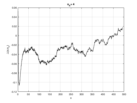
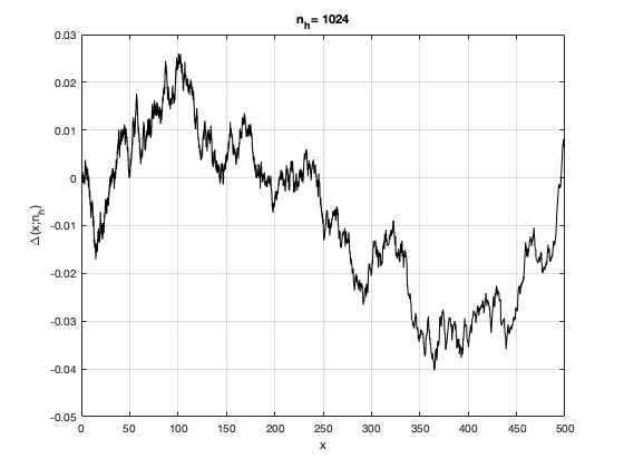
Figure 1: Log-tail approximation errors $\Delta(x;n_{h})$ for $n_{h}=4$ and $n_{h}=1024$.

2.2 A MAP test

Similarly to the Bayes test, we can construct the MAP test that rejects $\mathbf{H}_{0}^{h}$ if

$$\max_{t\in\mathcal{G}_{h}}\frac{1}{n_{h}}S\biggl{(}\frac{\hat{\theta}_{h,t}}{\sigma_{h}}\biggr{)}\geq t_{\alpha}^{M},$$

where $t_{\alpha}^{M}$ is defined as a solution to

$$\max_{\Theta\geq 0}\mathbf{P}_{\Theta}\biggl{\{}\max_{t\in\mathcal{G}_{h}}\frac{1}{n_{h}}S\biggl{(}\frac{\hat{\theta}_{h,t}}{\sigma_{h}}\biggr{)}>t_{\alpha}^{M}\biggr{\}}=\alpha.$$

Similarly to (9), $t_{\alpha}^{M}$ may be obtained from

$$\mathbf{P}\biggl{\{}\max_{t\in\mathcal{G}_{h}}\frac{S(\xi_{h,t})}{n_{h}}>t_{\alpha}^{M}\biggr{\}}=\alpha.$$

As to the limit distribution of $\max_{t\in\mathcal{G}_{h}}{S(\xi_{h,t})}/{n_{h}}$, as $h\rightarrow 0$, it follows immediately from (14) that

$$\max_{t\in\mathcal{G}_{h}}\frac{S(\xi_{h,t})}{n_{h}}\stackrel{{\scriptstyle\mathcal{D}}}{{=}}\frac{1+\varepsilon_{h}}{\varkappa},\ \text{as}\ h\rightarrow 0,$$ (19)

where $\varkappa$ is a standard exponential random variable and $\varepsilon_{h}$ satisfies (18).

3 Multi-level testing

3.1 MAP multi-level tests

A heuristic idea behind our construction of multi-level MAP tests for (3) is related to (19) and consists in computing a positive deterministic function $U_{h},\,h\in\mathcal{H},$ bounding from above the random process $\log(1/\varkappa_{h}),\,h\in\mathcal{H},$ where $\varkappa_{h}$ are independent standard exponential random variables. In other words, we are looking for $U_{h}$ such that

$$\zeta^{U}=\sup_{h\in\mathcal{H}}\biggl{[}\log\frac{1}{\varkappa_{h}}-U_{h}\biggr{]}$$

would be a non-degenerate random variable.

Let $q_{\alpha}^{U}$ be $\alpha$-value of $\zeta^{U}$, i.e., solution to

$$\mathbf{P}\bigl{\{}\zeta^{U}\geq q_{\alpha}^{U}\bigr{\}}=\alpha.$$

Therefore with (19), upper bounding random process $\log(1/\varkappa_{h})$ by $U_{h}$, we arrive at the test that rejects $\mathbf{H}_{0}$ if

$$\sup_{h\in\mathcal{H}}\biggl{\{}\max_{t\in\mathcal{G}_{h}}\log\biggl{[}\frac{1}{n_{h}}S\biggl{(}\frac{\hat{\theta}_{h,t}}{\sigma_{h}}\biggr{)}\biggr{]}-U_{h}\biggr{\}}\geq q_{\alpha}^{U}.$$ (20)

Computing $q_{\alpha}^{U}$ is based on the following simple fact. Assume that

$$K^{U}=\log\biggl{[}\sum_{h\in\mathcal{H}}{\rm e}^{-U_{h}}\biggr{]}<\infty.$$

Then

$$\sup_{h\in\mathcal{H}}\biggl{[}\log\frac{1}{\varkappa_{h}}-U_{h}\biggr{]}-K^{U}\stackrel{{\scriptstyle\mathcal{D}}}{{=}}\log\frac{1}{\varkappa}.$$ (21)

The proof of this identity is very simple. Indeed,

$$\begin{split}&\mathbf{P}\Bigl{\{}\sup_{h\in\mathcal{H}}\bigl{[}\log\frac{1}{\varkappa_{h}}-U_{h}\bigr{]}-K^{U}>x\Bigr{\}}\\ &\quad=1-\prod_{h\in\mathcal{H}}\mathbf{P}\Bigl{\{}\log\frac{1}{\varkappa_{h}}\leq U_{h}+x+K^{U}\Bigr{\}}\\ &\quad=1-\exp\biggl{\{}-\sum_{h\in\mathcal{H}}\exp\biggl{[}-x-U_{h}-K^{U}\biggr{]}\biggr{\}}=1-\exp[-\exp(-x)].\end{split}$$

Let us we denote

$$\bar{\pi}_{h}={\rm e}^{-U_{h}}\biggl{/}\sum_{h\in\mathcal{H}}{\rm e}^{-U_{h}},$$

then (21) can be rewritten in the following form:

Proposition 2.

Let $\bar{\pi}$ be a probability distribution on $\mathcal{H}$. Then

$$\sup_{h\in\mathcal{H}}\biggl{[}\log\frac{1}{\varkappa_{h}}+\log(\bar{\pi}_{h})\biggr{]}\stackrel{{\scriptstyle\mathcal{D}}}{{=}}\log\frac{1}{\varkappa}.$$ (22)

Therefore with the help of (21) we can compute $\alpha$-critical level $q_{\alpha}^{U}$ in (20)

$$q_{\alpha}^{U}=q_{\alpha}^{\varkappa}+K^{U},$$

where

$$q_{\alpha}^{\varkappa}=-\log\biggl{(}\log\frac{1}{1-\alpha}\biggr{)}$$

is $\alpha$-value of $\log(1/\varkappa)$.

Summarizing (see (20)), the MAP multi-level test rejects $\mathbf{H}_{0}$ if

$$\sup_{h\in\mathcal{H}}\bigl{\{}Z^{M}_{h}+\log(\bar{\pi}_{h})\bigr{\}}\geq q_{\alpha}^{\varkappa},$$ (23)

where

$$Z_{h}^{M}=\max_{t\in\mathcal{G}_{h}}\log\biggl{[}\frac{1}{n_{h}}S\biggl{(}\frac{\hat{\theta}_{h,t}}{\sigma_{h}}\biggr{)}\biggr{]}$$

and $\bar{\pi}$ is a probability distribution on $\mathcal{H}$.

In order to study the performance of this method, we analyze the type II error probability. For given $\{\rho,\tau:\rho\in\mathcal{H},\ \tau\in\mathcal{G}_{g}\}$ and $A\in\mathbb{R}^{+}$ define

$$\Theta_{\rho,\tau}(A)=\Bigl{\{}\theta_{h,t}:\theta_{\rho,\tau}=-A;\ \theta_{h,t}\geq 0,(h,t)\neq(\rho,\tau)\Bigr{\}}.$$ (24)

In other words, we consider the situation, where all shifts $\theta_{h,t}$ in (2) are positive except the only one. The position of the negative entry $\{\rho,\tau\}$ and its amplitude are unknown, but it is assumed that $\{\rho,\tau\}$ are random variables with the distribution defined by

• $\mathbf{P}\{\rho=h\}=\bar{\pi}_{h}$,

• $\mathbf{P}\{\tau=t|\rho=h\}=n_{h}^{-1}$,

where $\bar{\pi}$ is a probability distribution on $\mathcal{H}$ with a bounded entropy

$$H_{\bar{\pi}}=\sum_{h\in\mathcal{H}}\bar{\pi}_{h}\log\frac{1}{\bar{\pi}_{h}}.$$

In what follows, we will deal with priors $\bar{\pi}$ with large uncertainties assuming that $\bar{\pi}\rightarrow 0$, or more precisely, $\sup_{h\in\mathcal{H}}\bar{\pi}_{h}\rightarrow 0,$ but such that

$$\lim_{\bar{\pi}\rightarrow 0}\frac{1}{\log[H_{\bar{\pi}}]}\sum_{h\in\mathcal{H}}\bar{\pi}_{h}\biggr{|}H_{\bar{\pi}}-\log\frac{1}{\bar{\pi}_{h}}\biggr{|}=0.$$ (25)

In particular, we will consider the following class of prior distributions:

$$\bar{\pi}_{h}=\bar{\pi}_{h}^{\omega,\nu}=\nu\biggl{[}\frac{\log_{2}(1/h)}{\omega}\biggr{]}\bigg{/}\sum_{k=1}^{\infty}\nu\biggl{(}\frac{k}{\omega}\biggr{)}\approx\frac{1}{\omega}\nu\biggl{[}\frac{\log_{2}(1/h)}{\omega}\biggr{]}.$$ (26)

This class is characterized by the bandwidth $\omega>1$ and the probability density $\nu(x),\ x\in\mathbb{R}^{+}$, which is assumed to be continuous, bounded, and with

$$H_{\nu}=\int_{0}^{\infty}\nu(x)\log\frac{1}{\nu(x)}dx<\infty,\quad\int_{0}^{\infty}\nu(x)\log(x+1)\,dx<\infty.$$ (27)

A typical example of a such distribution is the uniform one that corresponds to $\nu(x)=1,\,x\in[0,1]$.

It is clear that $\bar{\pi}_{h}^{\omega,\nu}\rightarrow 0$ as $\omega\rightarrow\infty$ and that Condition (25) holds.

Let us begin with the case, where the prior distribution is known, the case of unknown $\bar{\pi}$ will be considered later in Section 4.

The type II error probability over $\Theta_{\rho,\tau}(A)$ of the MAP test (23) is defined as follows:

$$\beta^{M}_{\rho,\tau}(A)=\sup_{\Theta\in\Theta{\rho,\tau}(A)}\mathbf{P}_{\Theta}\Bigl{\{}\max_{h\in\mathcal{H}}\bigl{[}Z_{h}^{M}+\log(\bar{\pi}_{h})\bigr{]}\leq q_{\alpha}^{\varkappa}\Bigr{\}}.$$

Our goal is to study the average type II error probability

$$\bar{\beta}^{M}_{\bar{\pi}}(\mathbf{A})=\sum_{h\in\mathcal{H}}\frac{\bar{\pi}_{h}}{n_{h}}\sum_{t\in\mathcal{G}_{h}}\beta^{M}_{h,t}(A_{h}),$$

where here and below $\mathbf{A}=\{A_{h},\,h\in\mathcal{H}\}$.

Denote for brevity

$$R_{h}(q,H)=2[q+\log(n_{h})+H]-\log[4\pi(q+\log(n_{h})+H)]$$

and

$$\begin{split}\log^{*}(x)=&\log[\log(x)],\quad H^{*}_{\bar{\pi}}=\log(H_{\bar{\pi}}).\end{split}$$

The next theorem shows that $R_{h}(q_{\alpha}^{\varkappa},H_{\bar{\pi}})$ is a critical signal/noise ratio. Roughly speaking, this means that if

$$\frac{A_{h}}{\sigma_{h}}\stackrel{{\scriptstyle\bar{\pi}}}{{\leq}}\sqrt{R_{h}(q_{\alpha}^{\varkappa},H_{\bar{\pi}})}+x$$

for any given $x>0$, then the MAP multi-level test cannot discriminate between $\mathbf{H}_{0}$ and $\mathbf{H}_{1}$. Otherwise, if

$$\frac{A_{h}}{\sigma_{h}}\stackrel{{\scriptstyle\bar{\pi}}}{{\geq}}\sqrt{R_{h}(q_{\alpha}^{\varkappa},H_{\bar{\pi}})}+\sqrt{\epsilon H^{*}_{\bar{\pi}}},$$

for some $\epsilon>0$, then reliable testing is possible.

In the next theorem, $\mathbf{E}_{\bar{\pi}}$ stands for the expectation w.r.t. $\bar{\pi}$.

Theorem 3.

Suppose (25) holds. If for some $x\in\mathbb{R}$ and $\epsilon>0$

$$\lim_{\bar{\pi}\rightarrow 0}\frac{1}{H^{*}_{\bar{\pi}}}\mathbf{E}_{\bar{\pi}}\biggl{[}\biggl{(}\frac{A_{h}}{\sigma_{h}}-x\biggr{)}^{2}+\epsilon H^{*}_{\bar{\pi}}-R_{h}(q_{\alpha}^{\varkappa},H_{\bar{\pi}})\biggr{]}_{+}=0,$$ (28)

then

$$\lim_{\bar{\pi}\rightarrow 0}\bar{\beta}^{M}_{\bar{\pi}}(\mathbf{A})\geq(1-\alpha)[1-\Phi(x)].$$ (29)

If for some $\epsilon>0$

$$\lim_{\bar{\pi}\rightarrow 0}\frac{1}{H^{*}_{\bar{\pi}}}\mathbf{E}_{\bar{\pi}}\biggl{[}R_{h}(q_{\alpha}^{\varkappa},H_{\bar{\pi}})+2\sqrt{\epsilon H^{*}_{\bar{\pi}}}\frac{A_{h}}{\sigma_{h}}-\frac{A_{h}^{2}}{\sigma_{h}^{2}}\biggr{]}_{+}=0,$$ (30)

then

$$\lim_{\bar{\pi}\rightarrow 0}\bar{\beta}^{M}_{\bar{\pi}}(\mathbf{A})=0.$$ (31)

3.2 Multi-level Bayes tests

To construct these tests, let us consider the following statistics:

$$Z_{h}^{B}=\frac{1}{n_{h}}\sum_{t\in\mathcal{G}_{h}}S\biggl{(}\frac{\hat{\theta}_{h,t}}{\sigma_{h}}\biggr{)}-\log(n_{h})-\gamma+1,\ h\in\mathcal{H}.$$

When all $\theta_{h,t}=0$, in view of Theorem 2, these random variables are approximated by the family of independent and identically distributed random variables $\zeta^{\circ}_{h},h\in\mathcal{H}$, defined by (16). An important property of this family is provided by (13), which is used in our construction multi-level Bayes tests. More precisely, the multi-level Bayes test rejects $\mathbf{H}_{0}$ if

$$\sum_{h\in\mathcal{H}}\bar{\pi}_{h}\biggl{(}Z_{h}^{B}-\log\frac{1}{\bar{\pi}_{h}}\biggr{)}\geq q_{\alpha}^{\circ},$$

where $q_{\alpha}^{\circ}$ is $\alpha$-value of $\zeta^{\circ}$.

The type II error probability over $\Theta_{\rho,\tau}(A)$ (see (24)) is defined by

$$\beta^{B}_{\rho,\tau}(A)=\sup_{\Theta\in\Theta_{\rho,\tau}(A_{\rho})}\mathbf{P}_{\Theta}\biggl{\{}\sum_{h\in\mathcal{H}}\bar{\pi}_{h}\biggl{(}Z_{h}^{B}-\log\frac{1}{\bar{\pi}_{h}}\biggr{)}\leq q_{\alpha}^{\circ}\biggr{\}}$$

and our goal is to analyze the average type II error probability

$$\bar{\beta}^{B}_{\bar{\pi}}(\mathbf{A})=\sum_{h\in\mathcal{H}}\frac{\bar{\pi}_{h}}{n_{h}}\sum_{\tau\in\mathcal{G}_{h}}\beta^{B}_{h,\tau}(A_{h}).$$

Theorem 4.

Suppose (25) holds and for some $x\in\mathbb{R}$ and $\epsilon>0$

$$\lim_{\bar{\pi}\rightarrow 0}\frac{1}{H^{*}_{\bar{\pi}}}\mathbf{E}_{\bar{\pi}}\biggl{[}\biggl{(}\frac{A_{h}}{\sigma_{h}}-x\biggr{)}^{2}+\epsilon H^{*}_{\bar{\pi}}-R_{h}[\log(q_{\alpha}^{\circ}),H_{\bar{\pi}}]\biggr{]}_{+}=0,$$ (32)

then

$$\lim_{\bar{\pi}\rightarrow 0}\bar{\beta}^{B}_{\bar{\pi}}(\mathbf{A})\geq(1-\alpha)[1-\Phi(x)].$$ (33)

If for some $\epsilon>0$

$$\lim_{\bar{\pi}\rightarrow 0}\frac{1}{H^{*}_{\bar{\pi}}}\mathbf{E}_{\bar{\pi}}\biggl{[}R_{h}\bigl{[}\log(q_{\alpha}^{\circ}),H_{\bar{\pi}}\bigr{]}+2\sqrt{\epsilon H^{*}_{\bar{\pi}}}\frac{A_{h}}{\sigma_{h}}-\frac{A_{h}^{2}}{\sigma_{h}^{2}}\biggr{]}_{+}=0,$$ (34)

then

$$\lim_{\bar{\pi}\rightarrow 0}\bar{\beta}^{B}_{\bar{\pi}}(\mathbf{A})=0.$$ (35)

Remark.

Notice that as $\alpha\rightarrow 0$

$$\log(q_{\alpha}^{\circ})=(1+o(1))q_{\alpha}^{\varkappa}=(1+o(1))\log\frac{1}{\alpha}.$$

Therefore, since $H_{\bar{\pi}}\rightarrow\infty$ as $\bar{\pi}\rightarrow 0$, conditions (28) and (32) along with (30) and (34) are almost equivalent. This means that in the considered statistical problem there is no substantial difference between MAP and Bayes tests.

4 Adaptive multi-level tests

The main drawback of the MAP and Bayes tests is related to their dependence on the prior distribution $\bar{\pi}$ that is hardly known in practice. Therefore our next goal is to construct a test that, on the one hand, does not depend on $\bar{\pi}$, but on the other hand, has a nearly optimal critical signal-noise ratio.

In order to simplify our presentation, we will deal with the class of prior distributions $\bar{\pi}^{\omega,\nu}$ defined by (26). The entropy of $\bar{\pi}^{\omega,\nu}$ obviously satisfies

$$H_{\bar{\pi}^{\omega,\nu}}=\log(\omega)+H_{\nu}+o(1),\ \omega\rightarrow\infty,$$ (36)

and therefore denote for brevity

$$\widetilde{R}_{h}(q,\omega)=2[q+\log(n_{h})+\log(\omega)]-\log[4\pi(q+\log(n_{h})+\log(\omega)].$$ (37)

With (36), Condition (25) is checked easily and the next result follows immediately from Theorem 3.

Corollary 1.

If for some $x\in\mathbb{R}$ and $\epsilon>0$

$$\begin{split}\lim_{\omega\rightarrow\infty}\frac{1}{\log^{*}(\omega)}\mathbf{E}_{\bar{\pi}^{\omega,\nu}}\biggl{[}\biggl{(}\frac{A_{h}}{\sigma_{h}}-x\biggr{)}^{2}+\epsilon\log^{*}(\omega)-\widetilde{R}_{h}(q_{\alpha}^{\varkappa},\omega)\biggr{]}_{+}&=0,\end{split}$$

then

$$\lim_{\omega\rightarrow\infty}\bar{\beta}^{M}_{\bar{\pi}^{\omega,\nu}}(\mathbf{A})\geq(1-\alpha)[1-\Phi(x)].$$

If for some $\epsilon>0$

$$\begin{split}\lim_{\omega\rightarrow\infty}\frac{1}{\log^{*}(\omega)]}\mathbf{E}_{\bar{\pi}^{\omega,\nu}}\biggl{[}\widetilde{R}_{h}(q_{\alpha}^{\varkappa},\omega)+2\sqrt{\epsilon\log^{*}(\omega)}\frac{A_{h}}{\sigma_{h}}-\frac{A_{h}^{2}}{\sigma_{h}^{2}}\biggr{]}_{+}=0,\end{split}$$

then

$$\lim_{\omega\rightarrow\infty}\bar{\beta}^{M}_{\bar{\pi}^{\omega,\nu}}(\mathbf{A})=0.$$

In order to construct an adaptive test, let us compute a nearly minimal function $U_{h}$ in (21). We begin with

$$\psi_{0}(x)=1+\log(x),\quad x\in\mathbb{R}^{+},$$

and then iterate this function $m$ times

$$\psi_{l}(x)=\psi_{0}\bigl{[}\psi_{l-1}(x)\bigr{]},\ l=1,\ldots,m.$$

Finally, for given $\varepsilon\in(0,1)$, define

$$L^{m,\varepsilon}(k)=-\log\bigg{\{}\frac{1}{\varepsilon[\psi_{m}(k)]^{\varepsilon}}-\frac{1}{\varepsilon[\psi_{m}(k+1)]^{\varepsilon}}\biggr{\}},\ k\in\mathbb{Z}^{+}.$$ (38)

Since $\psi_{m}(1)=1$, it is clear that

$$\sum_{k=1}^{\infty}\exp[-L^{m,\varepsilon}(k)]=\frac{1}{\varepsilon}.$$

In what follows, we will make use of the following approximation of $L^{m,\varepsilon}(k)$ for large $k$. Denote (see (38))

$$\begin{split}&\widetilde{L}^{m,\varepsilon}(k)=-\log\bigg{[}-\frac{1}{\varepsilon}\frac{[d\psi_{m}(k)]^{-\varepsilon}}{dk}\biggr{]}=-\log\bigg{[}\frac{1}{[\psi_{m}(k)]^{1+\varepsilon}}\frac{d\psi_{m}(k)}{dk}\biggr{]}\\ &\qquad=\log(k)+\log[\psi_{0}(k)]+\cdots+\log[\psi_{m-1}(k)]+(1+\varepsilon)\log[\psi_{m}(k)].\end{split}$$ (39)

Since

$$\frac{d^{2}\psi_{m}(k)}{dk^{2}}\bigg{/}\frac{d\psi_{m}(k)}{dk}=O\biggl{(}\frac{1}{k}\biggr{)},$$

by the Taylor formula we obtain from (38)

$$\Delta^{m,\varepsilon}(k)=\widetilde{L}^{m,\varepsilon}(k)-{L}^{m,\varepsilon}(k)=O\biggl{(}\frac{1}{\psi_{m}(k)}\biggr{)}.$$ (40)

Figure 2 shows that ${L}^{m,\varepsilon}(k)$ and approximation errors $\Delta^{m,\varepsilon}(k)$.

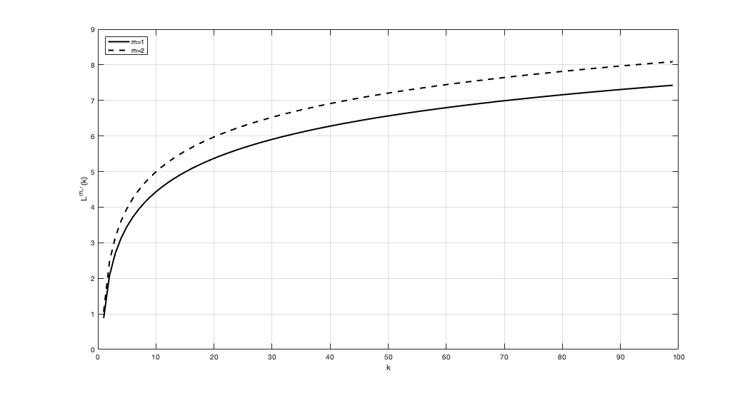
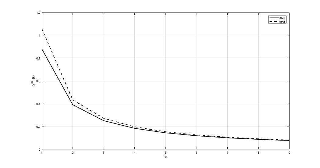
Figure 2: The functions $L^{m,\varepsilon}(\cdot)$ and the approximation errors $\Delta^{m,\varepsilon}(\cdot)$ for $m=1,2$ and $\varepsilon=0.1$.

Since $h\in\mathcal{H}=\{2^{-1},\ldots,2^{-k},\ldots\}$, we choose

$$U_{h}=L^{m,\varepsilon}[\log_{2}(1/h)]$$

and in view of (38) we arrive at the following prior distribution:

$${\Pi}_{h}=\frac{1}{\{\psi_{m}[\log_{2}(1/h)]\}^{\varepsilon}}-\frac{1}{\{\psi_{m}[\log_{2}(1/h)+1]\}^{\varepsilon}},\ h\in\mathcal{H}.$$

It is easy to check that the entropy of ${\Pi}$ is unbounded and this is why this distribution might be viewed as an improper prior.

The MAP test associated with ${\Pi}$ rejects $\mathbf{H}_{0}$ when

$$\max_{h\in\mathcal{H}}\bigl{\{}Z_{h}^{M}+\log\bigl{(}{\Pi}_{h}\bigr{)}\bigr{\}}\geq q_{\alpha}^{\varkappa}$$

and its type II error probability over $\Theta_{\rho,\tau}(A)$ (see (24)) is defined by

$$\beta_{\rho,\tau}^{\Pi}(A)=\sup_{\Theta\in\Theta_{\rho,\tau}(A)}\mathbf{P}_{\Theta}\Bigl{\{}\max_{h\in\mathcal{H}}\bigl{[}Z_{h}^{M}+\log({\Pi}_{h})\bigr{]}\leq q_{\alpha}^{\varkappa}\Bigr{\}}.$$

Denote for brevity

$$R^{+}(q_{\alpha}^{\varkappa},\omega)=\widetilde{R}(q_{\alpha}^{\varkappa},\omega)+\log^{*}(\omega),$$ (41)

where $\widetilde{R}(q_{\alpha},\omega)$ is defined by (37), and let

$$\bar{\beta}^{\Pi}_{\bar{\pi}^{\omega,\nu}}\bigl{(}\mathbf{A})=\sum_{h\in\mathcal{H}}\frac{\bar{\pi}_{h}^{\omega,\nu}}{n_{h}}\sum_{t\in\mathcal{G}_{h}}\beta^{\Pi}_{h,t}(A_{h})$$

be the average type II error probability.

Theorem 5.

If for some $x\in\mathbb{R}$ and $\epsilon>0$

$$\begin{split}\lim_{\omega\rightarrow\infty}\frac{1}{\log^{*}(\omega)}\mathbf{E}_{\bar{\pi}^{\omega,\nu}}\biggl{[}\biggl{(}\frac{A_{h}}{\sigma_{h}}-x\biggr{)}^{2}+\epsilon\log^{*}(\omega)-R_{h}^{+}(q_{\alpha}^{\varkappa},\omega)\biggr{]}_{+}&=0,\end{split}$$

then

$$\lim_{\omega\rightarrow\infty}\bar{\beta}^{\Pi}_{\bar{\pi}^{\omega,\nu}}(\mathbf{A})\geq(1-\alpha)[1-\Phi(x)].$$

If for some $\epsilon>0$

$$\begin{split}\lim_{\omega\rightarrow\infty}\frac{1}{\log^{*}(\omega)}\mathbf{E}_{\bar{\pi}^{\omega,\nu}}\biggl{[}R_{h}^{+}(q_{\alpha}^{\varkappa},\omega)+2\sqrt{\epsilon\log^{*}(\omega)}\frac{A_{h}}{\sigma_{h}}-\frac{A_{h}^{2}}{\sigma_{h}^{2}}\biggr{]}_{+}=0,\end{split}$$

then

$$\lim_{\omega\rightarrow\infty}\bar{\beta}^{\Pi}_{\bar{\pi}^{\omega,\nu}}(\mathbf{A})=0.$$

This theorem and Corollary 1 demonstrate that the critical signal-noise ratio of the adaptive test is only slightly greater, see (41), (by the additive term $\log^{*}(\omega)$) than the one of the MAP test that knows the prior distribution $\bar{\pi}^{\omega,\nu}$.

5 Appendix

5.1 Proof of Theorem 1

With a simple algebra we obtain

$$\begin{split}&\log\bigl{\{}\mathbf{E}\exp\bigl{[}{\rm i}tB_{h}(\xi)\bigr{]}\bigr{\}}=n_{h}\log\biggl{\{}\frac{1}{\sqrt{2\pi}}\int_{-\infty}^{\infty}\cos\biggl{[}\frac{tS(x)}{n_{h}}\biggr{]}{\rm e}^{-x^{2}/2}\,dx\\ &\qquad+\frac{\rm i}{\sqrt{2\pi}}\int_{-\infty}^{\infty}\sin\biggl{[}\frac{tS(x)}{n_{h}}\biggr{]}{\rm e}^{-{x^{2}}/{2}}\,dx\biggr{\}}\\ &\ =n_{h}\log\biggl{\{}1+\int_{-\infty}^{\infty}\biggr{[}\cos\biggl{[}\frac{t}{n_{h}}\biggl{(}\frac{1}{\Phi(x)}-1\biggr{)}\biggr{]}-1\biggl{]}\,d\Phi(x)\\ &\qquad+{\rm i}\int_{-\infty}^{\infty}\sin\biggl{[}\frac{t}{n_{h}}\biggl{(}\frac{1}{\Phi(x)}-1\biggr{)}\biggr{]}\,d\Phi(x)\biggr{\}}\\ &\ =n_{h}\log\biggl{\{}1+\int_{0}^{1}\biggl{\{}\cos\biggl{[}\frac{t}{n_{h}}\biggl{(}\frac{1}{u}-1\biggr{)}\biggr{]}-1\biggr{\}}\,du\\ &\qquad+{\rm i}\int_{0}^{1}\sin\biggl{[}\frac{t}{n_{h}}\biggl{(}\frac{1}{u}-1\biggr{)}\biggr{]}\,du\biggr{\}}\\ &\ =n_{h}\log\biggl{\{}1+\int_{0}^{\infty}\frac{1}{(1+u)^{2}}\biggl{[}\cos\biggl{(}\frac{tu}{n_{h}}\biggr{)}-1\biggr{]}\,du\\ &\qquad\qquad+{\rm i}\int_{0}^{\infty}\frac{1}{(1+u)^{2}}\sin\biggl{(}\frac{tu}{n_{h}}\biggr{)}\,du\biggr{\}}\\ &\ =n_{h}\log\biggl{\{}1+\frac{|t|}{n_{h}}\int_{0}^{\infty}\frac{\cos(u)-1}{(|t|/n_{h}+u)^{2}}\,du+\frac{{\rm i}t}{n_{h}}\int_{0}^{\infty}\frac{\sin(u)}{(|t|/n_{h}+u)^{2}}\,du\biggr{\}}.\end{split}$$ (42)

It is clear that as $n_{h}\rightarrow\infty$

$$\int_{0}^{\infty}\frac{\cos(u)-1}{(|t|/n_{h}+u)^{2}}\,du\rightarrow\int_{0}^{\infty}\frac{\cos(u)-1}{u^{2}}\,du=-\frac{\pi}{2}.$$ (43)

Let us choose $\epsilon_{h}<1$ such that

$$\lim_{h\rightarrow 0}\epsilon_{h}=0,\quad\lim_{h\rightarrow 0}\epsilon_{h}n_{h}=\infty.$$

Then we get by the Taylor formula

$$\begin{split}&\int_{0}^{\infty}\frac{\sin(u)}{(|t|/n_{h}+u)^{2}}\,du=\int_{0}^{\epsilon_{h}}\frac{\sin(u)}{(|t|/n_{h}+u)^{2}}\,du+\int_{\epsilon_{h}}^{\infty}\frac{\sin(u)}{(|t|/n_{h}+u)^{2}}\,du\\ &\qquad=\int_{0}^{\epsilon_{h}}\frac{u}{(|t|/n_{h}+u)^{2}}\,du+O\biggl{[}\int_{0}^{\epsilon_{h}}\frac{u^{3}}{(|t|/n_{h}+u)^{2}}\,du\biggr{]}\\ &\qquad\quad+(1+o(1))\int_{\epsilon_{h}}^{\infty}\frac{\sin(u)}{u^{2}}\,du\\ &\qquad=\log\bigg{(}1+\frac{\epsilon_{h}n_{h}}{|t|}\biggr{)}-\frac{\epsilon_{h}n_{h}}{(|t|+\epsilon_{h}n_{h})}\\ &\qquad\quad+(1+o(1))\int_{\epsilon_{h}}^{\infty}\frac{\sin(u)}{u^{2}}\,du+O(\epsilon_{h}^{2}).\end{split}$$ (44)

Next, integrating by parts, we obtain

$$\begin{split}\int_{x}^{\infty}\frac{\sin(z)}{z^{2}}\,dz=&-\int_{x}^{\infty}\frac{\sin(z)}{z}\,d\biggl{(}\log\frac{1}{z}\biggr{)}\\ =&\frac{\sin(x)}{x}\log\frac{1}{x}+\int_{x}^{\infty}\frac{z\cos(z)-\sin(z)}{z^{2}}\log\frac{1}{z}\,dz.\end{split}$$

Hence, as $x\rightarrow 0$

$$\begin{split}\int_{x}^{\infty}\frac{\sin(z)}{z^{2}}\,dz=&\log\frac{1}{x}+\int_{0}^{\infty}\frac{z\cos(z)-\sin(z)}{z^{2}}\log\frac{1}{z}\,dz+O\bigg{(}x^{2}\log\frac{1}{x}\biggr{)}\\ =&\log\frac{1}{x}+(1-\gamma)+O\bigg{(}x^{2}\log\frac{1}{x}\biggr{)},\end{split}$$

where $\gamma$ is Euler’s constant.

With this equation we continue (44) as follows:

$$\begin{split}\int_{0}^{\infty}\frac{\sin(u)}{(|t|/n_{h}+u)^{2}}\,du=\log\frac{1}{|t|}+\log(n_{h})-\gamma+O\biggl{(}\frac{|t|}{\epsilon_{h}n_{h}}\biggr{)}+O\biggl{(}\epsilon_{h}^{2}\log\frac{1}{\epsilon_{h}}\biggr{)}.\end{split}$$

Substituting this equation and (43) in (42), we get

$$\begin{split}\log\bigl{\{}\mathbf{E}\exp\bigl{[}{\rm i}tB_{h}(\xi)\bigr{]}\bigr{\}}=-\frac{\pi|t|}{2}+{\rm i}t\biggl{(}\log\frac{1}{|t|}+\log(n_{h})-\gamma\biggr{)}+o(1),\end{split}$$

thus, proving the theorem.

5.2 Proof of Theorem 3

I. A lower bound. By (22) we have for any given $x$

$$\begin{split}&\beta^{M}_{\rho,\tau}(A)\geq\mathbf{P}\biggl{\{}\biggl{[}\log\biggl{[}S\biggl{(}-\frac{A}{\sigma_{\rho}}+\xi_{\rho,\tau}\biggr{)}\biggr{]}-\log\frac{n_{\rho}}{\bar{\pi}_{\rho}}\biggr{]}\\ &\qquad\bigvee\biggl{[}\zeta_{\rho}-\log\frac{1}{\bar{\pi}_{\rho}}\biggr{]}\leq q_{\alpha}^{\varkappa}\biggr{\}}\mathbf{P}\biggl{\{}\max_{h\in\mathcal{H}}\biggl{[}\zeta_{h}-\log\frac{1}{\bar{\pi}_{h}}\biggr{]}\leq q_{\alpha}^{\varkappa}\biggr{\}}\\ &=\mathbf{P}\biggl{\{}S\biggl{(}-\frac{A}{\sigma_{\rho}}+\xi_{\rho,\tau}\biggr{)}\leq\exp\biggl{[}q_{\alpha}^{\varkappa}+\log\frac{n_{\rho}}{\bar{\pi}_{\rho}}\biggr{]}\biggr{\}}\\ &\quad\times\mathbf{P}\biggl{\{}\zeta_{\rho}\leq q_{\alpha}^{\varkappa}+\log\frac{1}{\bar{\pi}_{\rho}}\biggr{\}}\mathbf{P}\bigl{\{}\zeta\leq q_{\alpha}^{\varkappa}\bigr{\}}\\ &\geq(1-\alpha)^{1+\bar{\pi}_{\rho}}\mathbf{P}\biggl{\{}S\biggl{(}-\frac{A}{\sigma_{\rho}}+\xi_{\rho,\tau}\biggr{)}\leq\exp\biggl{[}q_{\alpha}^{\varkappa}+\log\frac{n_{\rho}}{\bar{\pi}_{\rho}}\biggr{]};\xi_{\rho,\tau}\geq x\biggr{\}}\\ &\geq(1-\alpha)^{1+\bar{\pi}_{\rho}}\mathbf{P}\bigl{\{}\xi_{\rho,\tau}\geq x\bigr{\}}\mathbf{1}\biggl{\{}S\biggl{(}-\frac{A}{\sigma_{\rho}}+x\biggr{)}\leq\exp\biggl{[}q_{\alpha}^{\varkappa}+\log\frac{n_{\rho}}{\bar{\pi}_{\rho}}\biggr{]}\biggr{\}}.\end{split}$$ (45)

Let $R(z)\geq 0$ be a solution to

$$S\Bigl{[}-\sqrt{R(z)}\Bigr{]}=z.$$

It is easy to check with the help of (7) that as $z\rightarrow\infty$

$$R(z)=2\log(z)-\log[4\pi\log(z)]+o(1).$$ (46)

Denote for brevity

$$r_{h}(q,u)=2\biggl{(}q+\log\frac{n_{h}}{u}\biggr{)}-\log\biggl{[}4\pi\biggl{(}q+\log\frac{n_{h}}{u}\biggr{)}\biggr{]}.$$

With (46) and the Markov inequality we obtain for any $\epsilon>0$

$$\begin{split}&\mathbf{E}_{\bar{\pi}}\biggl{[}\mathbf{1}\biggl{\{}S\biggl{(}-\frac{A_{h}}{\sigma_{h}}+x\biggr{)}\leq\exp\biggl{[}q_{\alpha}^{\varkappa}+\log\frac{n_{h}}{\bar{\pi}_{h}}\biggr{]}\biggr{\}}\biggr{]}\\ &\quad=1-\mathbf{E}_{\bar{\pi}}\biggl{[}\mathbf{1}\biggl{\{}S\biggl{(}-\frac{A_{h}}{\sigma_{h}}+x\biggr{)}>\exp\biggl{[}q_{\alpha}^{\varkappa}+\log\frac{n_{h}}{\bar{\pi}_{h}}\biggr{]}\biggr{\}}\biggr{]}\\ &\quad=1-\mathbf{E}_{\bar{\pi}}\biggl{[}\mathbf{1}\biggl{\{}\biggl{(}\frac{A_{h}}{\sigma_{h}}-x\biggr{)}^{2}-r_{h}(q_{\alpha}^{\varkappa},\bar{\pi}_{h})>o(1)\biggr{\}}\biggr{]}\\ &\quad\geq 1-\frac{1}{\epsilon H^{*}_{\bar{\pi}}}\mathbf{E}_{\bar{\pi}}\biggl{[}\biggl{(}\frac{A_{h}}{\sigma_{h}}-x\biggr{)}^{2}-r_{h}(q_{\alpha}^{\varkappa},\bar{\pi}_{h})+\epsilon H^{*}_{\bar{\pi}}\biggr{]}_{+}.\end{split}$$ (47)

With Condition (25) and simple algebra it is easy to check that

$$\lim_{\bar{\pi}\rightarrow 0}\frac{1}{H^{*}_{\bar{\pi}}}\mathbf{E}_{\bar{\pi}}\biggl{|}r_{h}(q_{\alpha}^{\varkappa},\bar{\pi})-R_{h}(q_{\alpha}^{\varkappa},H_{\bar{\pi}})\biggr{|}=0.$$

Therefore (29) follows from (45), (47) and the above equation.

II. An upper bound. Since $S(x)$ is a decreasing function, we have obviously for any $x\geq 0$

$$\begin{split}\bar{\beta}^{M}_{\bar{\pi}}(\mathbf{A})\leq&\mathbf{E}_{\bar{\pi}}\biggl{[}\mathbf{P}\biggl{\{}S\biggl{(}-\frac{A_{h}}{\sigma_{h}}+\xi\biggr{)}\leq\exp\biggl{[}q_{\alpha}^{\varkappa}+\log\frac{n_{h}}{\bar{\pi}_{h}}\biggr{]}\biggr{\}}\biggr{]}\\ \leq&\mathbf{E}_{\bar{\pi}}\biggl{[}\mathbf{P}\biggl{\{}S\biggl{(}-\frac{A_{h}}{\sigma_{h}}+\xi\biggr{)}\leq\exp\biggl{[}q_{\alpha}^{\varkappa}+\log\frac{n_{h}}{\bar{\pi}_{h}}\biggr{]};\xi\leq x\biggr{\}}\biggr{]}\\ +&\mathbf{E}_{\bar{\pi}}\biggl{[}\mathbf{P}\biggl{\{}S\biggl{(}-\frac{A_{h}}{\sigma_{h}}+\xi\biggr{)}\leq\exp\biggl{[}q_{\alpha}^{\varkappa}+\log\frac{n_{h}}{\bar{\pi}_{h}}\biggr{]};\xi>x\biggr{\}}\biggr{]}\\ \leq&\mathbf{E}_{\bar{\pi}}\biggl{[}\mathbf{1}\biggl{\{}S\biggl{(}-\frac{A_{h}}{\sigma_{h}}+x\biggr{)}\leq\exp\biggl{[}q_{\alpha}^{\varkappa}+\log\frac{n_{h}}{\bar{\pi}_{h}}\biggr{]}\biggr{\}}\biggr{]}+\mathbf{P}\bigl{\{}\xi>x\bigr{\}}.\end{split}$$

Next, with (46), the Markov inequality, and Condition (25) we get for any $\epsilon>0$

$$\begin{split}&\sum_{h\in\mathcal{H}}\bar{\pi}_{h}\mathbf{1}\biggl{\{}S\biggl{(}-\frac{A_{h}}{\sigma_{h}}+x\biggr{)}\leq\exp\biggl{[}q_{\alpha}^{\varkappa}+\log\frac{n_{h}}{\bar{\pi}_{h}}\biggr{]}\biggr{\}}\\ &\quad\leq\sum_{h\in\mathcal{H}}\bar{\pi}_{h}\mathbf{1}\biggl{\{}r_{h}(q_{\alpha}^{\varkappa},\bar{\pi}_{h})-\biggl{(}\frac{A_{h}}{\sigma_{h}}-x\biggr{)}^{2}>o(1)\biggr{\}}\\ &\quad\leq\frac{1}{\epsilon H^{*}_{\bar{\pi}}}\sum_{h\in\mathcal{H}}\bar{\pi}_{h}\biggr{[}r_{h}(q_{\alpha}^{\varkappa},\bar{\pi}_{h})-\biggl{(}\frac{A_{h}}{\sigma_{h}}-x\biggr{)}^{2}+\epsilon H^{*}_{\bar{\pi}}\biggr{]}_{+}\\ &\quad\leq\frac{1}{\epsilon H^{*}_{\bar{\pi}}}\sum_{h\in\mathcal{H}}\bar{\pi}_{h}\biggr{[}R_{h}(q_{\alpha}^{\varkappa},H_{\bar{\pi}})-\biggl{(}\frac{A_{h}}{\sigma_{h}}-x\biggr{)}^{2}+\epsilon H^{*}_{\bar{\pi}}\biggr{]}_{+}+o(1).\end{split}$$

To complete the proof, let us choose $x=\sqrt{\epsilon H^{*}_{\bar{\pi}}}$.

5.3 Proof of Theorem 4

A lower bound. For given $x$ and $\delta>0$ by (17) and (13), we obtain

$$\begin{split}&\beta^{B}_{\rho,\tau}(A)\geq\mathbf{P}\biggl{\{}\frac{\bar{\pi}_{\rho}}{n_{\rho}}S\biggl{(}-\frac{A}{\sigma_{\rho}}+\xi_{\rho,\tau}\biggr{)}+\zeta^{\circ}\leq q_{\alpha}^{\circ};\xi_{\rho,\tau}\geq x\biggr{\}}\\ &\quad\geq\mathbf{P}\biggl{\{}\frac{\bar{\pi}_{\rho}}{n_{\rho}}S\biggl{(}-\frac{A}{\sigma_{\rho}}+x\biggr{)}+\zeta^{\circ}\leq q_{\alpha}^{\circ};\xi_{\rho,\tau}\geq x\biggr{\}}\\ &\quad=\mathbf{P}\bigl{\{}\xi_{\rho,\tau}\geq x\bigr{\}}\mathbf{P}\biggl{\{}\zeta^{\circ}\leq q_{\alpha}^{\circ}-\frac{\bar{\pi}_{\rho}}{n_{\rho}}S\biggl{(}-\frac{A}{\sigma_{\rho}}+x\biggr{)}\biggr{\}}\\ &\quad\geq\mathbf{P}\bigl{\{}\xi_{\rho,\tau}\geq x\bigr{\}}\mathbf{P}\bigl{\{}\zeta^{\circ}\leq(1-\delta)q_{\alpha}^{\circ}\bigr{\}}\mathbf{1}\biggl{\{}\frac{\bar{\pi}_{\rho}}{n_{\rho}}S\biggl{(}-\frac{A}{\sigma_{\rho}}+x\biggr{)}\leq\delta q_{\alpha}^{\circ}\biggr{\}}.\end{split}$$

Similarly to (47), since $\bar{\pi}\rightarrow 0$, we get

$$\begin{split}&\mathbf{E}_{\bar{\pi}}\biggl{[}\mathbf{1}\biggl{\{}\frac{\bar{\pi}_{h}}{n_{h}}S\biggl{(}-\frac{A_{h}}{\sigma_{h}}+x\biggr{)}\leq\delta q_{\alpha}^{\circ}\biggr{\}}\biggr{]}\\ &\quad\geq 1-\frac{1}{\epsilon H^{*}_{\bar{\pi}}}\mathbf{E}_{\bar{\pi}}\biggl{[}\biggl{(}\frac{A_{h}}{\sigma_{h}}-x\biggr{)}^{2}+\epsilon H^{*}_{\bar{\pi}}-R_{h}[\log(\delta q_{\alpha}^{\circ}),H_{\bar{\pi}}]\biggr{]}_{+}\\ &\quad\geq 1-\frac{1}{\epsilon H^{*}_{\bar{\pi}}}\mathbf{E}_{\bar{\pi}}\biggl{[}\biggl{(}\frac{A_{h}}{\sigma_{h}}-x\biggr{)}^{2}+\epsilon H^{*}_{\bar{\pi}}-R_{h}[\log(q_{\alpha}^{\circ}),H_{\bar{\pi}}]\biggr{]}_{+}\\ &\quad\geq 1+o(1).\end{split}$$

So, since $\delta$ is arbitrary, (33) follows from the above inequalities.

An upper bound. Since $S(x)$ is decreasing, we get

$$\begin{split}\beta^{B}_{\rho,\tau}(A)\leq&\mathbf{P}\biggl{\{}\frac{\bar{\pi}_{\rho}}{n_{\rho}}S\biggl{(}-\frac{A}{\sigma_{\rho}}+\xi_{\rho,\tau}\biggr{)}+\zeta^{\circ}\leq q_{\alpha}^{\circ};\xi_{\rho,\tau}\geq x\biggr{\}}\\ +&\mathbf{P}\biggl{\{}\frac{\bar{\pi}_{\rho}}{n_{\rho}}S\biggl{(}-\frac{A}{\sigma_{\rho}}+\xi_{\rho,\tau}\biggr{)}+\zeta^{\circ}\leq q_{\alpha}^{\circ};\xi_{\rho,\tau}\leq x\biggr{\}}\\ \leq&\mathbf{P}\bigl{\{}\xi_{\rho,\tau}\geq x\bigr{\}}+\mathbf{P}\biggl{\{}\frac{\bar{\pi}_{\rho}}{n_{\rho}}S\biggl{(}-\frac{A}{\sigma_{\rho}}+x\biggr{)}+\zeta^{\circ}\leq q_{\alpha}^{\circ}\biggr{\}}.\end{split}$$ (48)

Next, for any given $x^{\circ}<q_{\alpha}^{\circ}$ we obtain with the help of the Markov inequality and (46)

$$\begin{split}&\mathbf{E}_{\bar{\pi}}\biggl{[}\mathbf{P}\biggl{\{}\frac{\bar{\pi}_{h}}{n_{h}}S\biggl{(}-\frac{A_{h}}{\sigma_{h}}+x\biggr{)}+\zeta^{\circ}\leq q_{\alpha}^{\circ}\biggr{\}}\biggr{]}\\ &\quad\leq\mathbf{E}_{\bar{\pi}}\biggl{[}\mathbf{P}\biggl{\{}\frac{\bar{\pi}_{h}}{n_{h}}S\biggl{(}-\frac{A_{h}}{\sigma_{h}}+x\biggr{)}+\zeta^{\circ}\leq q_{\alpha}^{\circ};\zeta^{\circ}<x^{\circ}\biggr{\}}\biggr{]}\\ &\qquad+\mathbf{E}_{\bar{\pi}}\biggl{[}\mathbf{P}\biggl{\{}\frac{\bar{\pi}_{h}}{n_{h}}S\biggl{(}-\frac{A_{h}}{\sigma_{h}}+x\biggr{)}+\zeta^{\circ}\leq q_{\alpha}^{\circ};\zeta^{\circ}\geq x^{\circ}\biggr{\}}\biggr{]}\\ &\quad\leq\mathbf{P}\bigl{\{}\zeta^{\circ}<x^{\circ}\}+\mathbf{E}_{\bar{\pi}}\biggl{[}\mathbf{1}\biggl{\{}\frac{\bar{\pi}_{h}}{n_{h}}S\biggl{(}-\frac{A_{h}}{\sigma_{h}}+x\biggr{)}\leq q_{\alpha}^{\circ}-x^{\circ}\biggr{\}}\biggr{]}\\ &\quad\leq\mathbf{P}\bigl{\{}\zeta^{\circ}<x^{\circ}\}+\frac{1}{\epsilon H^{*}_{\bar{\pi}}}\mathbf{E}_{\bar{\pi}}\biggl{[}R_{h}[\log(q_{\alpha}^{\circ}-x^{\circ}),H_{\bar{\pi}}]+\epsilon H^{*}_{\bar{\pi}}-\biggl{(}\frac{A_{h}}{\sigma_{h}}-x\biggr{)}^{2}\biggr{]}_{+}.\end{split}$$

Finally choosing $x=\sqrt{\epsilon H^{*}_{\bar{\pi}}}$ and combining this equation with (48), we complete the proof of (35).

5.4 Proof of Theorem 5

Let us consider

$$H\bigl{(}\bar{\pi}^{\omega,\nu},{\Pi}\bigr{)}=\sum_{h\in\mathcal{H}}\bar{\pi}^{\omega,\nu}_{h}\log\frac{1}{{\Pi}_{h}}.$$

One can check easily with (38)–(40) and (26) that as $\omega\rightarrow\infty$

$$\begin{split}&H\bigl{(}\bar{\pi}^{\omega,\nu},{\Pi}\bigr{)}=\log\frac{1}{\varepsilon}+\frac{1}{\omega}\sum_{k=1}^{\infty}\nu\biggl{(}\frac{k}{\omega}\biggr{)}L^{m,\varepsilon}(k)+o(1)=\log\frac{1}{\varepsilon}+o(1)\\ &+\int_{0}^{\infty}\nu(x)\biggl{[}\log(x\omega+1)+\sum_{s=0}^{m-1}\log[\psi_{s}(x\omega)]+(1+\varepsilon)\log[\psi_{m}(x\omega)]\biggr{]}\,dx.\end{split}$$

It is also clear in view of (27) that

$$\int_{0}^{\infty}\nu(x)\log(x\omega+1)\,dx=\log(\omega)+O(1)$$

and for any integer $s\geq 0$

$$\int_{0}^{\infty}\nu(x)\log[\psi_{s}(x\omega)]\,dx=\log[\psi_{s}(\omega)]+O(1).$$

Therefore as $\omega\rightarrow\infty$

$$H\bigl{(}\bar{\pi}^{\omega,\nu},{\Pi}\bigr{)}=\log(\omega)+(1+o(1))\log^{*}(\omega).$$ (49)

Next, with similar arguments we obtain

$$\begin{split}&\sum_{h\in\mathcal{H}}\bar{\pi}^{\omega,\nu}_{h}\biggl{[}H(\bar{\pi}^{\omega,\nu},{\Pi})-\log\frac{1}{{\Pi}_{h}}\biggr{]}_{+}\\ &\qquad=\int_{0}^{\infty}\nu(x)\Bigl{[}H(\bar{\pi}^{\omega,\nu},{\Pi})-\log(x\omega+1)\\ &\qquad\quad-(1+o(1))\log[\log(x\omega+1)+1]\Bigr{]}_{+}dx\\ &\qquad=\int_{0}^{\infty}\nu(x)\Bigl{[}\log(\omega)+(1+o(1))\log^{*}(\omega)]-\log(x\omega+1)\\ &\qquad\quad-(1+o(1))\log[\log(x\omega+1)+1]\Bigr{]}_{+}dx\\ &\qquad=\int_{0}^{\infty}\nu(x)\bigl{[}-\log(x+1)+o(1)\log^{*}(\omega)\bigr{]}_{+}dx=o(1)\log^{*}(\omega)].\end{split}$$ (50)

In view of (49) and (50) the rest of the proof is similar to the one of Theorem 3 and therefore omitted.

References

- [1] Baraud Y., Huet S., and Laurent B. (2005). Testing convex hypotheses on the mean of a Gaussian vector. Application to testing qualitative hypotheses on a regression function. Ann. Statist. 33, 214–257.
- [2] Bowman A. W., Jones M. C., and Gijbels I. (1998). Testing monotonicity of regression. J. Comput. Graph. Statist. 7, 489–500.
- [3] Burnashev M. and Bergamov I. (1990). On a problem of signal detection leading to stable distributions. Theory Probab. Appl. 35(3), 556–560.
- [4] Chetverikov D. (2019). Testing regression monotonicity in econometric models. Econometric Theory 35(4), 729–776
- [5] Dobrushin R. (1958). A statistical problem arising in the theory of detection of signals in the presence of noise in a multi-channel system and leading to stable distribution Laws. Theory Probab. Appl. 3(2), 161–173.
- [6] Dümbgen L., and Spokoiny V. (2001). Multiscale testing of qualitative hypotheses. Ann. Statist., 29, 124–152.
- [7] Durot C. (2003). A Kolmogorov-type test for monotonicity of regression. Statist. Probab. Lett. 63, 425–433.
- [8] Ghosal S., Sen A., and van der Vaart A. (2000). Testing monotonicity of regression. Ann. Statist. 28, 1054–1082.
- [9] Gijbels I., Hall, P., Jones M., and Koch I. (2000). Tests for monotonicity of a regression mean with guaranteed level. Biometrika 87, 663–673.
- [10] Hall P. and Heckman N. (2000). Testing for monotonicity of a regression mean by calibrating for linear functions. Ann. Statist. 28, 20–39.
- [11] Ingster Yu. I. and Suslina I. A. (2003). Nonparametric Goodness-of-Fit Testing Under Gaussian Models. Lecture Notes in Statistics 169. New York: Springer.
- [12] Mudholkar G. S. (1966). The integral of an invariant unimodal function over an invariant convex set – an inequality and applications. Proc. Amer. Math. Soc 17, 1327–1333.
- [13] Nolan J.P. (2016). Stable Distributions: Models for Heavy-Tailed Data. New York: Springer.
- [14] Pyke R. (1965). Spacings (with discussion). J. Roy. Statist. Soc. Ser. B 27(3), 395–449.
- [15] Schlee W. (1982). Nonparametric Tests of the Monotony and Convexity of Regression. In Non-parametric Statistical Inference, Amsterdam: North-Holland.
- [16] Tong Y. L. (1980). Probability Inequalities in Multivariate Distributions. 1st edition. . Academic Press.
- [17] Wang J. and Meyer M. (2011). Testing the monotonicity or convexity of a function using regression splines. Canad. J. Statist. 39, 89–107.