CME Iceberg Order Detection and Prediction

Abstract

We propose a method for detection and prediction of native and synthetic iceberg orders on Chicago Mercantile Exchange. Native (managed by the exchange) icebergs are detected using discrepancies between the resting volume of an order and the actual trade size as indicated by trade summary messages, as well as by tracking order modifications that follow trade events. Synthetic (managed by market participants) icebergs are detected by observing limit orders arriving within a short time frame after a trade. The obtained icebergs are then used to train a model based on the Kaplan–Meier estimator, accounting for orders that were cancelled after a partial execution. The model is utilized to predict the total size of newly detected icebergs. Out of sample validation is performed on the full order depth data, performance metrics and quantitative estimates of hidden volume are presented.

1 Introduction

On financial exchanges, an iceberg order is a limit order where only a fraction of the total order size (display quantity) is shown in the limit order book (LOB) at any one time (peak), with the remainder of volume hidden (Christensen and Woodmansey, 2013). When the peak is executed, the next part of the iceberg’s hidden volume (tranche or refill) gets displayed in the LOB. This process is repeated until the initial order is fully traded or cancelled.

The hidden volume, although not being directly observed, is de facto present in the LOB and hence can be traded against. This makes the detection of hidden liquidity a desirable goal for interested parties, e.g. traders and market makers.

In this paper we propose a method for detecting and predicting hidden liquidity on Chicago Mercantile Exchange (CME). The model is fit and assessed out of sample using historical data. We treat it both as a classification and a regression model and discuss relevant performance metrics.

1.1 Data

We had access to an almost week-long full order depth (FOD) LOB log of a September E-Mini S&P 500 futures contract, existing at that time under the ticker symbol ESU19, for the period from 2019-06-14, 11:00:00 CDT to 2019-06-21, 16:00:00 CDT. The chosen interval is especially interesting from a trading activity standpoint: as the front month contract ESM19 approaches its expiration, a majority of the open interest gets transferred onto the next one, creating an increased demand for hidden liquidity vehicles. Each order was described by a sequence of fields presented in table 1.

	Time	Order ID	Side	Action	Price	Volume
Possible values	Millisecond resolution	12-digit identifier	“B” (buy), “S” (sell)	“Limit” (new), “Modify” (update), “Delete”	Non-negative real	Non-negative integer

Table 1: Order log fields for the ESU19 data.

For more information about CME Market-by-Order book management, see (CME, 2019b).

In addition, trade summary messages (CME, 2019c) were present in the data. Each trade event against a resting order corresponded to a trade record in the log with the aforementioned fields, “Action” set to “Trade” and an extra field for the passive order ID.

This way, our algorithm works in the “offline” mode by reading a pre-recorded LOB log. Since it is not forward-looking, it can be easily modified to work with real-time streaming data.

1.2 CME Iceberg Orders

CME supports two types of iceberg orders: native and synthetic (CME, 2019a).

Native

icebergs are managed by the exchange itself. All new tranches are submitted as modifications of the initial order; this means that the original order ID is preserved throughout the whole lifetime of the iceberg. Additionally, trades against these orders may sometimes be larger in volume than the current resting size, as indicated by trade summary messages.

Synthetic

icebergs are submitted by independent software vendors (ISV), whose infrastructure is physically separated from the exchange. ISV’s split the initial iceberg order, submit new tranches and track their execution. These tranches are indistinguishable from usual limit orders submitted by other participants.

Detecting native icebergs is conceptually easy since a) the order ID does not change until the iceberg is fully executed or cancelled; and b) trade summary messages include actual trade volumes, which may be larger than the resting display quantity. Thus an unambiguous and accurate detection is possible. Synthetic icebergs, on the other hand, being identical to non-iceberg orders in how they are processed by the exchange, can only be detected heuristically and relying on a set of assumptions, which are introduced further.

2 Existing Literature Overview

For a good literature overview see (Christensen and Woodmansey, 2013, p. 7). In particular, some authors had access to order logs in which iceberg orders were explicitly identified, so that an unambiguous reconstruction of both displayed and hidden LOB’s was possible, e.g. by (Frey and Sandås, 2017) for XETRA exchange. There are a few articles that provide hidden liquidity estimates — see (Hautsch and Huang, 2010, p. 5) and (Christensen and Woodmansey, 2013, p. 7) for such lists. These estimates differ between authors, exchanges and instrument types, ranging from 2% (Fleming et al., 2018) to 52% (Moro et al., 2009). That being said, most of the papers were published almost a decade ago, so one may argue that contemporary markets have different hidden volume properties.

To our knowledge, there are virtually no articles that have the premise of simultaneous iceberg detection and prediction in the same setting as ours, with the exception of (Christensen and Woodmansey, 2013), who propose a solution to the very problem which the authors of the present paper are concerned with. Their approach consists of the following three phases:

1. Series of tranches are identified in the data as belonging to larger iceberg orders (the “detection” step).

2. Using the detected icebergs, a statistical model is fit that captures the correspondence between the peak size and the total iceberg size (the “learning” step).

3. The detection step is repeated, but a new iceberg order is detected, a prediction of the total size of the iceberg is made using the model obtained at the previous step (the “prediction” step).

We adapt this detection–learning–prediction scheme for our work, albeit with the following notable differences:

• The authors did not have the access to the FOD MBO data at the time of writing. In particular, the order ID for each action or trade was not available, yet that drastically changes the logic of the detection step.

• No distinction between synthetic and native icebergs is made. Namely, it is assumed that trades can sometimes be larger than the size of the resting order being traded, what is specific for native icebergs; however, iceberg tranches arrive as new limit orders, and that is an attribute of synthetic icebergs.

• During the learning phase, a bivariate Gaussian kernel density estimate of peak and total size is built, which is then optimised for the global maximum given a peak size. For the purpose of prediction, where only one value of the total size corresponding to the maximum probability given a peak size is necessary, this complication is questionable as a simpler model is sufficient. Kernel density estimate may be desired if the algorithm operates on instruments with a relatively low daily trading volume, and this is not the case with our data. In addition, by omitting this step we don’t have to resort to numerical methods when optimizing for conditional maxima.

• All incomplete icebergs — i.e. those, that were cancelled before being fully executed — are not included into the learning phase. However, our calculations show that more than half of all synthetic icebergs are cancelled, thus it is highly desirable to include the information about incomplete executions into the model.

3 Detection

3.1 Native Icebergs

Native iceberg orders enter the book as limit orders which may or may not be traded upon arrival. After the initial limit order volume is fully traded, the next part of the iceberg order appears in the book. Crucially, when the iceberg has its displayed quantity refreshed (by means of an update action), the refreshed order will have the same order ID as the original order. Moreover, any trades involving the iceberg order will indicate the total volume of trade, including the hidden part of the iceberg. Using these two properties it is then fairly easy to detect a sequence of new–trade–update–delete actions that forms an iceberg. In particular, we might be interested in update actions that correspond to new iceberg tranches, as well as in determining the peak size and in calculating the total iceberg size.

We would like to illustrate the process with an example. Consider the data presented in table 2.

Time	Order ID	Side	Action	Price	Volume	Affected
14:05:33.416	645764830354	S	Trade	2931.75	2	645764830338
14:05:33.416	645764830354	S	Trade	2931.75	10	645764830339
14:05:33.416	645764830354	S	Limit	2931.75	6	-
14:05:33.416	645764830360	B	Trade	2931.75	8	645764830354
14:05:33.416	645764830354	S	Modify	2931.75	7	-
14:05:33.416	645764830361	B	Trade	2931.75	3	645764830354
14:05:33.416	645764830354	S	Modify	2931.75	4	-
14:05:33.416	645764830362	B	Trade	2931.75	2	645764830354
14:05:33.416	645764830354	S	Modify	2931.75	2	-
14:05:33.416	645764830363	B	Trade	2931.75	1	645764830354
14:05:33.416	645764830354	S	Modify	2931.75	1	-
14:05:33.416	645764830365	B	Trade	2931.75	1	645764830354
14:05:33.416	645764830354	S	Modify	2931.75	9	-
14:05:33.416	645764830366	B	Trade	2931.75	1	645764830354
14:05:33.416	645764830354	S	Modify	2931.75	8	-
14:05:33.416	645764825841	B	Trade	2931.75	1	645764830354
14:05:33.416	645764830354	S	Modify	2931.75	7	-
14:05:33.417	645764830382	B	Trade	2931.75	9	645764830354
14:05:33.417	645764830354	S	Modify	2931.75	5	-
14:05:33.417	645764830390	B	Trade	2931.75	5	645764830354
14:05:33.417	645764830354	S	Delete	2931.75	5	-

Table 2: Sample native iceberg order log data. Grouped are the orders related to the same tranche.

1. Order #645764830354 enters the book and immediately gets traded at 2931.75 for the total of 12 units of volume. The remainder — 6 units — is placed at the same level. At that point we do not know whether the order has any hidden liquidity or not. Moreover, assuming that it does, the peak size cannot be precisely determined; but since $12+6=18$, it is one of the divisors of 18 greater or equal than 6, i.e. 6, 9 or 18.

2. The next trade has volume 8 which is larger than the resting volume of 6. This is sufficient to mark order #645764830354 as an active iceberg.

3. The next tranche volume is 7. Note that $8-6=2$ units of volume were traded against a tranche that had not entered the book. This means that the peak size can be determined precisely as $7+(8-6)=9$. The trade could have been large enough to consume several hidden tranches.

4. The next several trades are smaller in volume than the resting order. The trade initiated by order #645764830365 is equal to the resting volume of 1. Consequently, the next modify action is seen to refresh the visible volume by the peak size of 9 (which agrees with the previous calculations).

5. Finally, the last update action has volume 5, which, accounting for the hidden trade of $9-7=2$ results in peak size of 7. The trade for 5 units completes the sequence as no more refresh messages is seen and the order is deleted from the book.

Overall, the iceberg has a total volume of 43, 4 tranches with peak sizes 9, 9, 9 and 7, correspondingly, and the display quantity equal to 9.

The process of parsing the action stream can be conveniently formalised as a finite state machine, see fig. 1.

To recap the detection phase, an iceberg enters the book as a new limit order, possibly following a sequence of trades. It is then traded, and usually — but not always — each trade corresponds to one trade summary message, in which case it is followed by an update action, specifying the currently resting order volume. If more than one trade messages are seen before the next update action, then this should be accounted for. Moreover, all price adjustments which move the order to the top of the book are not disseminated by the exchange, meaning that even after the placement the order can again act as an aggressive order and initiate a trade. If at this point the order is deleted from the book or traded so that the trade volume is never greater than the resting volume, it is marked as “ordinary” and removed from consideration. On the other hand, once a trade larger than the resting volume is detected, or the order is fully traded but then modified to have non-zero volume again, then the order is marked as an iceberg. The trade–modify cycle then continues until the order is completely executed or cancelled, resulting in its deletion from the book.

In addition to tracking the transitions through the state space, we are interested in calculating the following quantities:

• the total volume $V_{\text{total}}$ is conveniently computed as the sum of all traded volume $V_{T}$ (which may exceed the sum of limit and/or update volumes), plus any volume $V_{D}$ that is explicitly deleted;

• the currently resting volume $V_{R}$ is simply the last modify action volume $V_{M}$;

• the peak size $V_{\text{peak}}$ is determined iteratively:

  • If the iceberg order enters the book directly as a limit order, then the limit order volume is indeed the peak size.

  • If a series of trades precedes the limit order placement, then $V_{L}=V_{\text{peak}}-V_{T}\bmod V_{\text{peak}}$. Therefore, $V_{T}-kV_{\text{peak}}=V_{\text{peak}}-V_{L}$ for some $k\in\mathbb{N}_{0}$, from which we get

    $$V_{\text{peak}}=\frac{V_{T}+V_{L}}{k+1}=\frac{V_{T}+V_{L}}{d},\quad d=1,\ldots,V_{T}+V_{L},\ V_{\mathrm{peak}}\in\{n\in\mathbb{N}:n\geq V_{L}\}.$$

    If more than one admissible $V_{\text{peak}}$ values are found, then the following heuristics apply.

    • If the first tranche is traded for exactly the resting volume, the following update message unambiguously identifies the peak size.

    • If the trade volume is greater than the resting volume, then

      $$V_{\text{peak}}=V_{M}+(V_{T}-V_{R})\bmod V_{\text{peak}}^{*},$$

      where $V_{\text{peak}}^{*}$ is one of previously computed values. Only the values that satisfy this equation are kept.

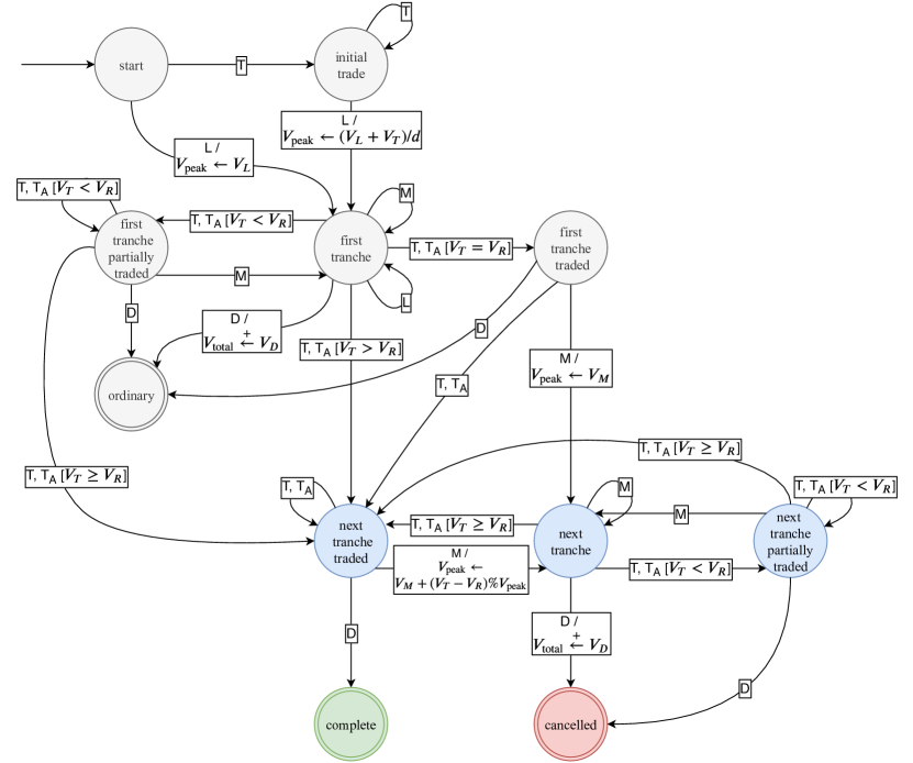
Figure 1: The grammar of native icebergs. The nodes correspond to states of the finite state machine, the edges — to order actions: new (L), update (M), trade (T), “affected” trade (T_A), delete (D). Trades T are initiated by the iceberg order, while “affected” trades T_A — by other incoming orders. An optional condition is specified in square brackets; a side effect is specified after the slash (/). Different volumes $V_{\cdot}$ refer to the iceberg’s peak volume $V_{\text{peak}}$, total volume $V_{\text{total}}$, current resting volume $V_{R}$ and the order’s trade ($V_{T}$), delete ($V_{D}$), modify ($V_{M}$) volumes. Node colours represent the status of the action sequence being tracked: grey for non-iceberg (“ordinary”), blue for active (all statuses starting with “next tranche…”), green for complete and red for cancelled.

3.2 Synthetic Icebergs

Unlike native icebergs, synthetic icebergs are managed by ISVs. After a tranche is fully executed, the ISV is expected to refill the display quantity with a new limit order. Since the ISV infrastructure is located outside the exchange, a short non-constant delay (dubbed $dt$) is expected between the corresponding “delete” and “new” actions. This idea is also exploited in (Christensen and Woodmansey, 2013), although their explanation was different. Additionally, we assume that new tranches arrive to the same price level as the initial tranche, and their volumes are expected to be equal to the initial tranche volume as well, which is taken to be the iceberg display quantity. It should be reiterated that we only detect orders that have constant peak size. Under the current model it is impossible to detect synthetic icebergs with varying peak sizes or price levels. This in particular implies that if the iceberg is not a multiple of the display quantity, the last tranche will be smaller than all the previous tranches in volume, hence its detection using the current approach does not seem to be possible.

If a tranche is executed, but no refill orders follow within $dt$, the iceberg is considered complete. If a tranche is placed and later cancelled, the whole iceberg is considered cancelled (incomplete).

One complication is that if the activity in the LOB is high (as in the case with E-Mini S&P 500 contracts), more than one order of the target volume may arrive on the same price level within $dt$. Our very strong assumption is that the next tranche arrives faster than any other new limit order, so for each tranche there is only one child. A more sophisticated model would account for all possible children tranches and somehow average the volume later on. Another complication is that when several limit orders of the same price and size get executed and deleted from the book simultaneously, the next tranche can be “linked” to any of those. Repeated over several trades, this produces a tree of possible tranches. Every path from all leaves to the root (a chain) is a possible iceberg. See table 3 and the resulting graph in fig. 2 for an illustration.

Time	Order ID	Side	Action	Price	Volume	Affected
18:22:12.00	1	S	Limit	1000	2	-
18:22:12.01	101	B	Trade	1000	2	1
18:22:12.01	1	S	Delete	1000	2	-
18:22:12.02	2	S	Limit	1000	2	-
18:22:12.04	4	S	Limit	1000	2	-
18:22:12.04	5	S	Limit	1000	2	-
18:22:13.00	102	B	Trade	1000	2	2
18:22:13.00	2	S	Delete	1000	2	-
18:22:13.01	3	S	Limit	1000	2	-
18:22:13.00	103	B	Trade	1000	2	4
18:22:13.00	104	B	Trade	1000	2	5
18:22:13.00	4	S	Delete	1000	2	-
18:22:13.00	5	S	Delete	1000	2	-
18:22:13.01	6	S	Limit	1000	2	-
18:22:14.00	7	S	Limit	1000	2	-
18:22:15.00	105	B	Trade	1000	2	3
18:22:15.00	106	B	Trade	1000	2	6
18:22:15.00	107	B	Trade	1000	2	7
18:22:15.00	3	S	Delete	1000	2	-
18:22:15.00	6	S	Delete	1000	2	-
18:22:15.00	7	S	Delete	1000	2	-
18:22:15.01	8	S	Limit	1000	2	-
18:22:16.00	108	B	Trade	1000	2	8
18:22:16.00	8	S	Delete	1000	2	-
18:22:16.01	9	S	Limit	1000	2	-
18:22:16.50	109	B	Trade	1000	2	9
18:22:16.50	9	S	Delete	1000	2	-

Table 3: Artificial data to demonstrate synthetic iceberg detection. For this example, $dt$ was set to 0.3 seconds. Limit order #1 gets traded and removed from the book. The following limit order #2 arriving within a third of a second becomes the next tranche in the iceberg chain. Note that orders #4 and #5 do not arrive within $dt$ and, since there were no more trades, start two new chains. After they get traded simultaneously, order #6 arrives within $dt$, thus becoming the next tranche. The process continues until all orders are removed from the book.

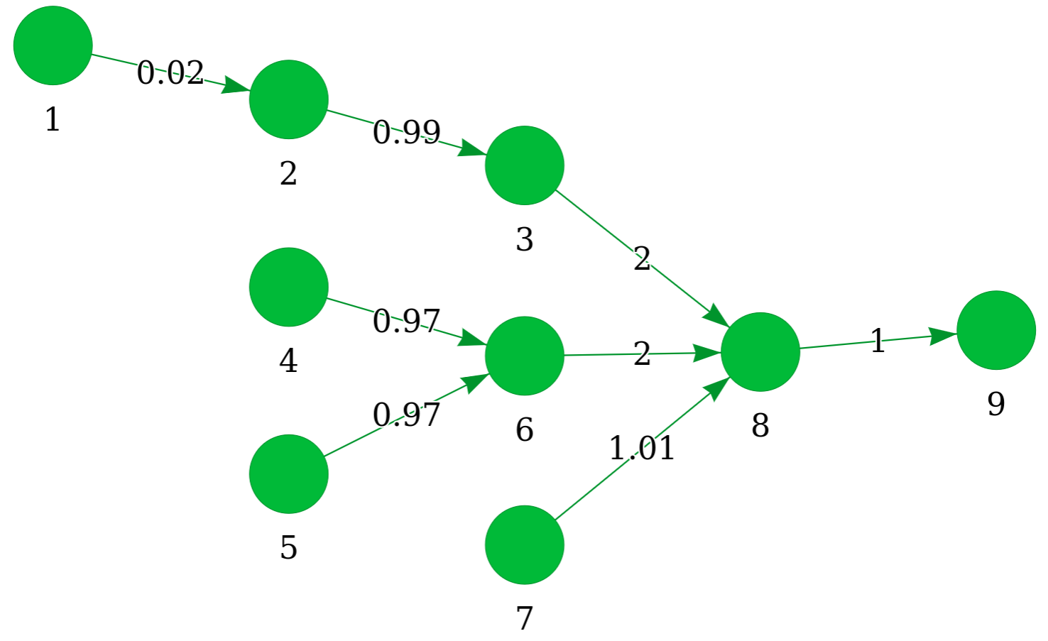
Figure 2: An iceberg tranche tree corresponding to table 3. Node labels are order IDs. Edge labels are time in seconds between subsequent tranches — note that these are different from $dt$ as a tranche can remain indefinitely long in the book after its placement. The iceberg consists of either 3, 4 (two chains) or 5 tranches.

We are also interested in computing the following related quantities:

• the peak size $V_{\text{peak}}$ is trivially set to be equal to the volume of the initial tranche;

• the total volume $V_{\text{total}}$ could have been calculated as the sum of the tranche volumes if there was only one tranche chain per iceberg. In general, however, there are more and the total volume has to be aggregated in some way. We propose the following options:

  • the average total volume of all chains $\mathcal{V}^{\text{all}}$;

  • the average total volume of chains of unique length $\mathcal{V}^{\text{unique}}$;

  • the total volume of the longest chain $\mathcal{V}^{\text{longest}}$.

4 Learning

4.1 Kaplan–Meier estimation

Having detected sufficiently many iceberg orders, we would like to build a model that yields a prediction of the total iceberg size. Although it is clearly not the most advanced in terms of predictive power, we elaborate on the model proposed in (Christensen and Woodmansey, 2013). Namely, for each of $P$ unique detected peak sizes, a distribution of possible total sizes is estimated; then, given the peak size $V_{\text{peak}}=p$ of a previously unseen iceberg, “the best” total volume (in terms of conditional mean, median or mode) is returned as a prediction.

More precisely, from now on let $V_{p}$ denote a random variable representing the total volume of an iceberg with peak size $p$. Then for each value of $p$ we are interested in estimating the distribution of $V_{p}$. While a trivial empirical distribution might suffice, our experiments show that a significant amount of synthetic icebergs are cancelled before being completely executed (see fig. 5). Hence for some icebergs only a lower bound on their total volume is known: for the $i$-th iceberg, $v_{i}\geq c_{i},\ c_{i}\in\mathbb{N}$. From the point of view of survival analysis, these are censored observations. Usually survival analysis deals with the so-called “time to event data”: the primary interest is the time until the onset of an event for each member of the analysed group. If only upper (or lower, or both) bounds on time, but not exact event times, are known, the observations are considered censored. Instead of discarding these, it is possible to construct estimators that incorporate the uncertainty associated with censoring. In our case, accumulated iceberg volumes play the role of time to event durations, so the task is to estimate the distribution of $V_{p}$ for each $p$ using random right-censored data.

The proportion of cancelled native icebergs is much smaller, and, in fact, could be disregarded for the purpose of distribution estimation. Nevertheless, we would like to utilise the same approach to simplify the analysis and to make the direct comparison between native and synthetic iceberg estimates possible.

The standard approach for a non-parametric distribution estimation of censored data is to use the Kaplan–Meier estimate (Kaplan and Meier, 1958). Let $F_{p}(v)$ be the cumulative distribution function of $V_{p}$, then $S_{p}(v)=1-F_{p}(v)$ is its survival function. Also define (for the given $p$) 00.00.0000

unique volumes of all detected icebergs sorted in ascending order,

the number of complete icebergs of volume $u_{j}$, where $j=1,\ldots,K$,

the total number of both complete and incomplete icebergs of volumes $u_{j},\ldots,u_{K}$. Then from the general theory of survival analysis it is known (Kalbfleisch and Prentice, 2002) that the maximum likelihood estimate of $S_{p}$ is

$$\hat{S}_{p}(v)=\prod_{j:u_{j}\geq v}\left(1-\frac{d_{j}}{n_{j}}\right).$$ (1)

4.2 Weighted Kaplan–Meier estimation for synthetic icebergs

For synthetic icebergs estimation (1) cannot be performed directly, because, given a tranche tree, there is no unambiguous way to calculate the total iceberg size. Instead, we propose a weighting scheme that assigns weights to each chain within a tranche tree. Given the $i$-th tranche tree with $h_{i}$ chains of unique length, the weights are

$$w_{i,\ell}=1/h_{i},\quad\ell\in 1:h_{i}.$$

A weight can be also interpreted as a probability of the total iceberg volume being equal to the accumulated tranche chain volume. Speaking in terms of Bayesian inference, we assign uniform probabilities because there is no prior knowledge that would affect our preference for a particular chain. Then for the purpose of calculating $\hat{S}_{p}(v)$, instead of $d_{j},n_{j}$, their weighted counterparts $\tilde{d}_{j}$, $\tilde{n}_{j}$ are computed. Formally, given the definition $\left\{u_{j}\right\}_{j=1,\ldots,K}$ above, let $\{v_{i,\ell}\}_{\ell=1,\ldots,h_{i}}$ denote a set of unique volumes of the $\ell$-th chain of the $i$-th tranche tree. Then

$$\tilde{d}_{j}=\sum_{i\in C}\sum_{\ell\in H_{i}}w_{i,\ell},\quad H_{i}=\left\{\ell:v_{i,\ell}=u_{j}\right\},$$

where $C$ is a set of indices of all complete icebergs and $H_{i}$ is a set of tranche chain indices of the $i$-th iceberg, having total volumes equal to $u_{j}$. $\tilde{n}_{j}$ are computed similarly. Of course, when each tranche tree consists of only one chain, all weights are equal to 1 and we have $\tilde{d}_{j}=d_{j}$ and $\tilde{n}_{j}=n_{j}$. Since $V_{p}$ only takes discrete values for all $p$, we finally obtain the weighted estimate

$$\hat{S}_{p}(u_{j})=\prod_{k=1}^{j}\left(1-\frac{\tilde{d}_{k}}{\tilde{n}_{k}}\right).$$

From $\hat{S}_{p}$ an estimate of the probability mass function $f_{p}(u_{j})=\mathsf{P}(V_{p}=u_{j})$ can be obtained in a trivial way. One notable problem with this estimate is that if $d_{K}=0$, then $S_{p}(u_{K})\neq 0$ and the probabilities do not sum up to 1. This is fixed trivially by normalising the probabilities.

5 Prediction

The prediction step starts from detecting first several tranches of an iceberg: for native icebergs, this might be any moment when the iceberg becomes “active”, for synthetic icebergs this number is an algorithm parameter with a default value of 3. If the peak size $p$ is precisely detected, a prediction of the total volume might be done.

5.1 Native Icebergs

For native icebergs we make predictions in terms of the conditional mean and median. In addition, a different prediction is made based on 3 highest conditional probabilities. For a fixed iceberg, let $v_{r}$ denote the currently accumulated volume up to, but not including, tranche number $r$ and let $\mathscr{V}_{p}=\left\{u_{j}:u_{j}>v_{r}\right\}_{j=1,\ldots,K_{p}}$ be the constrained optimization space. Then define

• mean prediction based on

  $$\mathsf{E}(V_{p}\mid V_{p}>v_{r})=\frac{1}{\mathsf{P}(V_{p}>v_{r})}\sum_{u\in\mathscr{V}_{p}}u\,\mathsf{P}(V_{p}=u)=\left(\sum_{u\in\mathscr{V}_{p}}f_{p}(u)\right)^{-1}\sum_{u\in\mathscr{V}_{p}}uf_{p}(u)$$

  and defined as

  $$\hat{v}^{\text{mean}}=\left(\sum_{u\in\mathscr{V}_{p}}\hat{f}_{p}(u)\right)^{-1}\sum_{u\in\mathscr{V}_{p}}u\hat{f}_{p}(u),$$

  rounded to the nearest integer;

• median prediction as

  $$\hat{v}^{\text{median}}=\max\left\{u_{J}:\sum_{j=1}^{J}\hat{f}_{p}(u_{j})\leq 0.5,\quad u_{j}\in\mathscr{V}_{p}\;\forall j=1,\ldots,\left|\mathscr{V}_{p}\right|\right\};$$

• $k$ best mode predictions as the $k$-th order statistic

  $$\hat{v}^{\text{mode}(k)}=u_{(k)},$$

  where the order of $u_{(1)},\ldots,u_{(\left|\mathscr{V}_{p}\right|)}$ is given by $\hat{f}_{p}(u_{(1)})\geq\dots\geq\hat{f}_{p}(u_{(\left|\mathscr{V}_{p}\right|)})$. Tied volumes are taken in ascending order.

5.2 Synthetic Icebergs

Once again, consider a fixed iceberg and an associated tranche tree. Let $v_{\ell,r}^{\prime}$ denote the currently accumulated volume for the $\ell$-th chain up to and including tranche number $r$. Then our prediction is

$$\hat{v}_{\ell}^{\text{mode}}=\operatorname*{argmax}_{u\in\mathscr{V}_{p}^{\prime}}\hat{f}_{p}(u),\quad\mathscr{V}_{p}^{\prime}=\left\{u_{j}:u_{j}\geq v_{\ell,r}^{\prime}\right\}_{j=1,\ldots,K_{p}},$$

where $\mathscr{V}_{p}^{\prime}$ is the constrained optimization space and $K_{p}$ is the number of unique total icebergs sizes with peak $p$. For the sake of brevity we do not report other possible estimates, as they do not differ much. The predicted total volume $\hat{v}_{\ell}^{\text{mode}}$ is aggregated across the chains of the iceberg in question as

• the average total volume of all chains $\hat{\mathcal{V}}^{\text{all}}$;

• the average total volume of chains of unique length $\hat{\mathcal{V}}^{\text{unique}}$;

• the total volume of the longest chain $\hat{\mathcal{V}}^{\text{longest}}$.

6 Evaluation

Given an estimate of $\hat{f}_{p}(v)$ and previously unseen data, the model can be evaluated both as a binary classifier and as a regression. In the discussion below, we assume that the prediction algorithm was run, producing a set of complete icebergs.

• For classification, our null hypothesis is “there is no hidden liquidity”. In the context of synthetic icebergs, it means that the iceberg is complete and no more tranches will follow. In the context of native icebergs, it means the last seen tranche can only be traded for the volume not exceeding its currently visible volume, and that no more tranches will follow. Since the full information on a particular iceberg execution is available after we run the prediction algorithm (each iceberg is eventually complete), the true total volume is known and hence the classification results can be summarised in a confusion matrix, from which we compute the standard classification metrics: accuracy, precision, recall and F1 score.

• Regression performance metrics show the degree to which the prediction is different from the true total volume.

The details of evaluation are slightly different for native and synthetic icebergs, and are given below. We hope that the level of details is sufficient so that there is no ambiguity of how the particular results were obtained.

6.1 Native Icebergs

Naturally, a prediction can be done each time the optimization space gets smaller — after a trade or a new tranche arrival. To match the case of synthetic icebergs as closely as possible, we decided to evaluate the prediction results only after each new tranche. The metrics defined below are calculated across the whole set of icebergs, so we reintroduce the appropriate indexation.

Let $\hat{v}_{i,r}^{\cdot}$ denote the estimated total size at tranche $r$ (where “$\cdot$” can be any of the “mean”, “median” or “mode”), $v_{i,r}$ — the actual accumulated volume up to, but not including, tranche $r$, $p_{i,r}$ — the peak size, and $R_{i}$ — the set of $i$-th iceberg tranches.

Classification

After a new tranche $r$ arrives, the accumulated volume is $v_{i,r}+p_{i,r}$. Hence if $v_{i,r}+p_{i,r}<v_{i}$, then the hypothesis is rejected (the true result is “negative”); consequently if $v_{i,r}+p_{i,r}<\hat{v}_{i,r}^{\cdot}$, then the outcome is “true negative”, otherwise it is “false positive”; and vice versa. For $\text{mode}(1),\ldots,\text{mode}(k)$ predictions, consider the prediction true if at least of the them was true.

Regression

Compute the residuals $e_{i,r}^{\cdot}=v_{i}-\hat{v}_{i,r}^{\cdot}$, $r\in R_{i}$. For $\text{mode}(1),\ldots,\text{mode}(k)$ predictions, select the residual that has a minimum absolute value. Use the residuals to calculate the standard regression metrics:

$$\mathrm{MAE} =\frac{1}{\left|R\right|}\sum_{i\in C}\sum_{r\in R_{i}}\left|e_{i,r}^{\cdot}\right|,$$ (2)

$$\mathrm{RMSE} =\sqrt{\frac{1}{\left|R\right|}\sum_{i\in C}\sum_{r\in R_{i}}\left(e_{i,r}^{\cdot}\right)^{2}},$$ (3)

where $R={\displaystyle\bigcup_{i\in C}}R_{i}$ and $C$ is the set of complete icebergs.

6.2 Synthetic Icebergs

For each complete iceberg with index $i$, the set of test tranches $R_{i}$ was formed by walking the tranche tree, starting from the root tranche, visiting each tranche only once and avoiding short chains (by default, of length less than three). Then the evaluation metrics were calculated as described below.

Let $\hat{\mathcal{V}}_{i,r}^{\cdot}$ denote the predicted total size and $\mathcal{V}_{i,r}^{\cdot}$ — the actual accumulated volume of the $i$-th iceberg up to and including tranche $r$, both quantities suitably aggregated — e.g. having “all”, “unique” or “longest” in place of the “$\cdot$”.

Classification

• For the last tranche $r_{\max}$, if $\hat{\mathcal{V}}_{i,r_{\max}}^{\cdot}=\mathcal{V}_{i,r_{\max}}^{\cdot}$, then the case is true positive, otherwise it is a false positive.

• For all but the last tranche ($r<r_{\max}$), if $\hat{\mathcal{V}}_{i,r}^{\cdot}>\mathcal{V}_{i,r}^{\cdot}$, then the case is true negative, otherwise it is a false negative.

Regression

Compute the residuals $e_{i,r}^{\cdot}=\hat{\mathcal{V}}_{i,r}^{\cdot}-\mathcal{V}_{i,r_{\max}}^{\cdot},\ r\in R_{i}.$ Use equations (2) and (3) to compute the regression metrics.

7 Results

We estimated $f_{p}(v)$ on one day of ESU19 (E-Mini S&P 500 futures contract) FOD LOB log data: from 2019-06-18, roughly 16:45:00 CDT, to 2019-06-19, 16:00:00 CDT; for synthetic icebergs, $dt$ was set to 0.3 seconds. The choice of parameters and training intervals is empirical and may be optimised further, but this falls outside of the scope of this article. Our evidence suggests that it is reasonable to include at least one trading session into the learning phase, thus capturing different order flow regimes throughout the day (see e.g. (Bouchaud et al., 2018, chapter 4)).

The following figures were produced using the data for the aforementioned period. For synthetic icebergs, the longest chain volume aggregation is used.

7.1 LOB Log Statistics

Figure 4 summarises the distribution of actions. Figure 4 shows the distribution of trade volumes.

Figure 3: Action distribution.

Figure 4: Trade volume distribution.

7.2 Detection Results

Fig. 5 shows the proportion of completed and cancelled icebergs of both types.

(a) Synthetic icebergs

(b) Native icebergs

Figure 5: Iceberg completion state distribution on ESM19 (E-Mini S&P 500) futures FOD LOB log data (2019/̄06/̄18 16:45:00 CDT – 2019/̄06/̄19 16:00:00 CDT).

The proportion of iceberg orders to all orders on one trading day is shown in fig. 6 in terms of both volume and number of orders. In case of synthetic icebergs, the results depend on the minimum number of tranches per iceberg — that is, the number of tranches after which their sequence is considered an iceberg. By increasing this parameter, we decrease the false positive rate at the cost of disregarding all icebergs of shorter lengths.

We divide the total volume of all iceberg orders by the total traded volume of all orders (like e.g. (Frey and Sandås, 2017) do), and not the total daily limit order volume. This ratio makes more sense because only executed icebergs can be detected, which surely constitute only a fraction of all resting hidden volume. We estimate that 4% of all traded volume is contributed by native icebergs, while the volume contributed by synthetic icebergs ranges from 3.3 to 14.3%, depending on the minimum number of tranches. This is in agreement with some of the results reported in the literature as alluded to earlier in section 2.

Moreover, as (Fleming et al., 2018) note, usually there is no hidden depth, but when it is present, it is substantial. This is especially true for native icebergs, that constitute 0.06% of all orders by number, but 4% by volume; see fig. 6.

In addition, the following size-related distributions are estimated:

• Trade volume (fig. 7). At least with native icebergs, we confirm the finding of (Christensen and Woodmansey, 2013) that order sizes to be multiples of 5, like 15, 25, 50 or 100 as can be seen in the right panel — this might be inidicative of a human bias.

• Peak volume (fig. 9).

• Number of tranches per iceberg (fig. 9).

(a) By volume

(b) By number of orders. Synthetic iceberg order tranches are counted either as one order, "s. (as one)", or separate orders, "s. (all tranches)"

Figure 6: Proportion of iceberg orders to all orders on one day.

(a) Density

(b) Individual probabilites (cutoff at 100 units)

Figure 7: Order size distribution.

Figure 8: Peak volume distribution.

Figure 9: Number of tranches distribution.

Figure 10 visualises summary statistics related to the distributions of the number of tranches, the peak size and the total volume per order. Note that the total volume of both native and synthetic icebergs is significantly different from the the size of all limit orders. Also, the median total volume is, in fact, identical for native and synthetic icebergs (being equal to 6), but the means are different due to some native icebergs having an extremely large size.

Figure 10: Summary of the distributions of the number of tranches per iceberg, the peak size and the total volume per order. The lower and upper hinges correspond to the first and third quartiles. The whiskers extend from the lower / upper hinge to the minimum / maximum value, respectively. The middle bar is the median, while the red diamond dot is the mean.

Lastly, fig. 11 shows the distribution of arrival time differences between subsequent tranches. Zero values are discarded for the purpose of drawing the plot, but they amount to 4.71% and 38.94% of all values for synthetic and native icebergs, correspondingly. If the initial tranche is not considered, then it can be seen that the majority of tranches arrive less than one second after the previous tranche (before being traded). This suggests that the proposed detection algorithm is more suitable as an input to other trading algorithms, rather than a signal to a day trader, who would not be able to react sufficiently fast.

(a) Native icebergs

(b) Synthetic icebergs

Figure 11: Tranche arrival time difference distributions (for values strictly greater than zero). It is instructive to compare two cases: when the initial tranche is included into and excluded from consideration — it might take longer time to execute the first tranche of an iceberg after its initial placement, but the following tranches get traded more rapidly.

7.3 Prediction Results

After the model was trained, its predictive ability was evaluated out of sample using the data for the period from 2019-06-19 16:45:00 CDT to 2019-06-20 16:45:00 CDT. An extensive study of the model robustness is required to claim its applicability on other instruments and time spans; we leave this out of the scope of this article.

Synthetic icebergs

The classification performance is summarised in tables 4 and 5. $\hat{\mathcal{V}}^{\mathrm{all}}$ and $\hat{\mathcal{V}}^{\mathrm{unique}}$ volume aggregation methods showed similar results (about 1% difference in the classification metrics). For the sake of brevity, only $\hat{\mathcal{V}}^{\mathrm{all}}$ and $\hat{\mathcal{V}}^{\mathrm{longest}}$ are displayed. The algorithm demonstrates a fair performance as indicated by the $\approx 70\%$ accuracy, although it is mainly contributed by the true negatives (the prediction that the iceberg is not complete). This is especially true in the case of the “all chains” aggregation. When checking for the equality $\hat{\mathcal{V}}_{r_{\max}}^{\mathrm{\cdot}}=\mathcal{V}_{r_{\max}}^{\cdot}$, taking the longest chain gives a better result, because $\hat{\mathcal{V}}_{r_{\max}}^{\mathrm{longest}}$ is not averaged and thus is always an integer. It is instructive to check the magnitude of the prediction error — the equality $\hat{\mathcal{V}}_{r_{\max}}^{\mathrm{\cdot}}=\mathcal{V}_{r_{\max}}^{\cdot}$ might not hold, but not by a large margin. Indeed, as the Regression section of table 4 demonstrates, the prediction is off by 1.78 units of volume on average.

		All chains average	Longest chain
Classification	Accuracy	68.95%	67.54%
	Precision	52.66%	49.95%
	Recall	41.47%	83.67%
	F1 score	46.40%	62.56%
Regression	MAE	1.78 (22.55%)	2.15 (24.94%)
	RMSE	3.94 (49.85%)	4.52 (52.37%)

Table 4: Evaluation metrics for synthetic icebergs. Percentages for regression are given relatively to the mean total volume.

	All chains average			Longest chain
	Actual complete	Actual incomplete		Actual complete	Actual incomplete
Predicted complete	3621 (13.44%)	3255 (12.08%)		7305 (27.12%)	7318 (27.17%)
Predicted incomplete	5110 (18.97%)	14952 (55.51%)		1426 (5.29%)	10889 (40.42%)

Table 5: Confusion matrices for synthetic icebergs.

Native icebergs

Of the total number of native icebergs (see fig. 5), 33 icebergs with non-unique peak size values were filtered out, leaving 98% of the initial amount used to estimate the total volume distribution.

Tables 6 and 7 summarise the predictive performance on native icebergs. Mode ($k$) columns refer to the metrics and confusion matrices computed using $k$ best mode predictions. For the sake of brevity, we only provide median and mode (3) confusion matrices as those averages have demonstrated the best results. As with synthetic icebergs, high accuracy values are mainly contributed by a large number of true negatives. Note that regression results are worse compared to the case of synthetic icebergs, which can possibly be explained by the smaller sample size.

		Mean	Median	Mode (1)	Mode (2)	Mode (3)
Classification	Accuracy	82.69%	58.31%	72.55%	88.15%	90.21%
	Precision	33.33%	19.22%	26%	73.03%	83.91%
	Recall	4.83%	47.59%	35.86%	44.83%	50.34%
	F1 score	8.43%	27.38%	30.14%	55.56%	62.93%
Regression	MAE	94.60 (97.87%)	89.40 (92.49%)	99.66 (103.14%)	69.66 (72.07%)	61.79 (63.92%)
	RMSE	217.08 (224.58%)	234.45 (242.55%)	239.22 (247.49%)	204.35 (211.41%)	190.43 (197.01%)

Table 6: Evaluation metrics for native icebergs. Percentages for regression are given relatively to the mean total volume.

	Median			Mode (3)
	Actual complete	Actual incomplete		Actual complete	Actual incomplete
Predicted complete	69 (7.85%)	290 (33.02%)		73 (8.31%)	14 (1.59%)
Predicted incomplete	76 (8.65%)	443 (50.45%)		72 (8.2%)	719 (81.89%)

Table 7: Confusion matrices for native icebergs.

8 Discussion and Future Work

We have proposed an algorithm for detection and prediction of both native and synthetic iceberg orders on CME. It can work with streaming data or with pre-recorded data in a suitable format equally well. The learning phase relies on a set of standard mathematical methods which are simple enough, so that they can be invoked from a corresponding statistical library or implemented from scratch. The detection results agree with some of the ones found in the literature. The prediction performance is fair given the simplicity of the model and can be improved further.

8.1 Detection

Detection of native icebergs is straightforward as the information disseminated by the exchange is sufficient to reliably determine the sequence of tranches that constitute an iceberg order.

On the other hand, detecting synthetic icebergs is conceptually more complicated and can only be attempted by relying on various heuristics. One inherent limitation of the proposed model is that the next tranche is expected to arrive earlier than any other limit orders for the same price and volume combination after a trade. In network graph terms, each node cannot have more than one child. This limitation may possibly be overcome by considering more complex graphs where each tranche is allowed to have more than one child, although at present it is unclear how to proceed with consistent inference in that case. The value of $dt$ parameter can be optimised using cross-validation.

That being said, for an end user interested in predictions, it may not matter at all whether the detected limit orders are a part of an iceberg order or not. Generally speaking, an order flow pattern gets detected, for which a satisfactory prediction can be made. This information can in turn be used as an input to trading algorithms.

8.2 Learning and prediction

For learning, the employed Kaplan–Meier estimate is arguably too simplistic. However, it improves the approach of (Christensen and Woodmansey, 2013), since it additionally accounts for the fact that many synthetic icebergs get cancelled before being fully executed. As simple as it is, the model does possess satisfactory predictive power and we hope that the present results will serve as a baseline for predictions using more advanced models.

There is much space for improvement of the learning and prediction procedures. One possibility is to optimize algorithm parameters, e.g. by using statistical techniques such as $k$-fold validation or bootstrap. Alternatively, for synthetic icebergs a better choice would be to utilize a semi-parametric relative risk (Cox) model and include covariates into the analysis, which would make the prediction more accurate. For native icebergs a variety of models are available as we are not restricted to the methods of survival analysis.

References

- Bouchaud et al. (2018) Bouchaud, J.-P., Bonart, J., Donier, J., and Gould, M. 2018. Trades, Quotes and Prices: Financial Markets Under the Microscope. Cambridge University Press.
- Christensen and Woodmansey (2013) Christensen, H. and Woodmansey, R. 2013. Prediction of Hidden Liquidity in the Limit Order Book of GLOBEX Futures. The Journal of Trading 8:68–95.
- CME (2019a) CME 2019a. Market by Order (MBO). https://www.cmegroup.com/education/market-by-order-mbo.html. Accessed: 2019-07-15.
- CME (2019b) CME 2019b. MDP 3.0 - Market by Order - Book Management. https://www.cmegroup.com/confluence/display/EPICSANDBOX/MDP+3.0+-+Market+by+Order+-+Book+Management. Accessed: 2019-07-15.
- CME (2019c) CME 2019c. MDP 3.0 - Trade Summary. https://www.cmegroup.com/confluence/display/EPICSANDBOX/MDP+3.0+-+Trade+Summary. Accessed: 2019-07-15.
- Fleming et al. (2018) Fleming, M., Mizrach, B., and Nguyen, G. 2018. The microstructure of a US Treasury ECN: The BrokerTec platform. Journal of Financial Markets 40:2–22.
- Frey and Sandås (2017) Frey, S. and Sandås, P. 2017. The Impact of Iceberg Orders in Limit Order Books. Quarterly Journal of Finance 07:1750007.
- Hautsch and Huang (2010) Hautsch, N. and Huang, R. 2010. A statistical model for detecting hidden liquidity. https://www.wiwi.hu-berlin.de/de/forschung/irtg/lvb/research/veranstaltungen/Hejnice2010/talks2010/Ruihong_Huang.
- Kalbfleisch and Prentice (2002) Kalbfleisch, J. and Prentice, R. 2002. The Statistical Analysis of Failure Time Data (Wiley Series in Probability and Statistics). Wiley-Interscience, 2 edition.
- Kaplan and Meier (1958) Kaplan, E. L. and Meier, P. 1958. Nonparametric Estimation from Incomplete Observations. Journal of the American Statistical Association 53:457–481.
- Moro et al. (2009) Moro, E., Vicente, J., Moyano, L. G., Gerig, A., Farmer, J. D., Vaglica, G., Lillo, F., and Mantegna, R. N. 2009. Market impact and trading profile of hidden orders in stock markets. Physical review. E, Statistical, nonlinear, and soft matter physics 80:066102.