Clock Error Analysis of Common Time of Flight based Positioning Methods

Abstract

Today, many applications such as production or rescue settings rely on highly accurate entity positioning. Advanced Time of Flight (ToF) based positioning methods provide high-accuracy localization of entities. A key challenge for ToF based positioning is to synchronize the clocks between the participating entities.
This paper summarizes and analyzes ToA and TDoA methods with respect to clock error robustness. The focus is on synchronization-less methods, i.e. methods which reduce the infrastructure requirement significantly. We introduce a unified notation to survey and compare the relevant work from literature. Then we apply a clock error model and compute worst case location-accuracy errors. Our analysis reveals a superior error robustness against clock errors for so called Double-Pulse methods when applied to radio based ToF positioning.

I Introduction

The ability to locate a device’s position is highly valuable in our modern and connected world. A considerable amount of research has therefore been conducted on that field, most recently in particular in the area of Time of Flight (ToF) based positioning. In a typical ToF setup, radio signals are used to estimate distances between so called Anchor and Tag nodes. Anchors have known positions and

Tags are to be located. There are two main approaches in ToF, which lead to different solving algorithms. The first one is Time of Arrival (ToA) which measures the sending and receiving time of a signal and is using these values to calculate a distance between two devices. For instance, in a 2D space the distances of one Tag to three Anchors are required to locate the Tag with multilateration algorithms [1]. In ToA the time of signal transmission as well as time of arrival has to be measured. In this basic version, all Anchors and Tags need to have synchronized clocks to perform the measurement.

The second approach is Time Difference of Arrival (TDoA) which measures the difference of signal arrivals. For instance, in a 2D space a signal sent from a Tag which is arriving at three different Anchors can be located by hyperbolic solver algorithms [2]. TDoA approaches do not require the time of signal transmission. Only the differences of the arrival times of the signal at the Anchors need to be known. Unlike the ToA case, this requires the Anchors to be synchronized among each other. No synchronization between Anchors and Tag is needed.

To have synchronized clocks is a considerable infrastructure requirement and, therefore, alternative methods to do synchronization-less ToA and TDoA have been developed [3, 4, 5, 6, 7]. Moreover, the fact that some of these methods work with radio waves, some with ultrasound is posing different requirements on the tolerable clock accuracy. The goal of this work is to analyze the relevant ToA and TDoA methods from the field of synchronization-less ToF. To achieve this, an error model is defined and applied to the approaches in order compare them against each other and to point out commonalities and differences.

The rest of the paper is organized as follows. First we will introduce the error model (Section II). Then both, ToA and TDoA methods will be presented in Section III and IV respectively. Finally, in Section V, a comparison and conclusion are given.

II Unified Error Model

Our error model is inspired by the works of Neirynck et al. [8] and Tschirschnitz and Wagner [6]. We adopt and optimize their underlying principle to make it applicable to the methods we assess in this paper.

II-A Clock Drift and Synchronization

Every clock contains imperfections, making it run at an inconstant rate. No existing clock is able to keep the perfect time [9]. Since ToF-based methods rely on the measurements of signals propagating with high speeds such as the speed of sound or the speed of light ($c$), clock imperfections make the runtime measurements inaccurate.

To reach a better understanding of clock errors, their deviation is typically described in the parts-per notation which is in the following in the order of magnitude of millions, hence Parts per Million (ppm) [10]. The parts-per notation specify the ratio of how many clock ticks the current clock-value is expected to deviate from the real time. As notation for the rest of this paper we introduce the symbol of $\epsilon_{A}$ to describe the clock error of device or oscillator $A$. For quartz oscillators a typical value for $\epsilon$ is $\pm 20$ ppm as defined in IEEE802.15.4 [11].

The current time $\hat{t}$ of device $A$ can therefore be expressed as:

$$\hat{t}:=t\cdot(1+\epsilon_{A})$$

$t$ is the ideal, error-free clock counter value and $\hat{t}$ is the error-affected counterpart.

Since in this paper we focus on ToF, which implies measurement of propagation of radio waves, clock counter precision needs to be below nanoseconds. For instance, $1$ns corresponds to $\approx 0.3$m of signal propagating with the speed of light.

A typical assumption in the field of ToF is that the drift of a specific clock is constant to allow measurements with the same clock error $\epsilon$ for some time [8].

II-B Measurement Errors and Multipath

The accuracy of time of flight measurements can be affected by additional error factors. The two most relevant factors are Non Line of Sight (NLoS) errors and multipath-propagation effects.

Multipath-Propagation Effect

The multipath-effect describes the fact that electromagnetic signals can reach a receiver on multiple paths. They can be reflected by walls or other obstacles for instance. As a consequence, a measured signal propagation time is not always that of the shortest possible path between the emitter and the receiver. However, for accurate distance measurements, the identification of the direct signal path, the so called primary signal is essential.

NLoS Error

NLoS errors occur if the direct path between a sender and a receiver is blocked by a material with different propagation properties than for example air. The signal traveling on the direct path between sender and receiver goes through the obstacle before reaching the antenna of the receiver. The obstacle changes the propagation speed.

As a consequence of having such material changes in real-world settings, it is impossible to make accurate assumptions about the signals traveling speed between the sender and the receiver. Moreover, NLoS scenarios make the identification of the primary signal under multipath-propagation harder.

Though the previously described problems have high relevance, we assume in the following Line of Sight (LoS) scenarios where the measurement errors can be neglected.

A more detailed description and analysis of those effects can be found in [12].

III Time of Arrival

Having defined this error-model we can now apply it to the relevant ToF methods from the state of the art. We will group the analyzed methods into ToA and TDoA, beginning with the former one.

III-A Simple Time-of-Arrival

The simplest ToF setup imaginable would be the one of simple Time-of-Arrival (simple-ToA). Simple-ToA consists of two devices $A$ and $B$ between which one signal is exchanged (compare Fig. 1). This signal sent by $A$ is timestamped (using $A$s clock) at the moment of transmission as well as when it is received at $B$ (using $B$s clock). If we now consider for a moment the synchronization between the devices clocks to be perfect, the difference between $A$ and $B$s timestamps would resemble the exact ToF between both.

$$d_{AB}=t_{2}-t_{1}$$ (1)

Then the distance between both could be calculated as:

$$\overline{AB}=c\cdot d_{AB}$$ (2)

Problems arise if we now reconsider the calculation under the assumption that synchronization is not provided and also when considering the presence of clock drift effects (like described in Section II-A). For example, even if we assume to have both clocks to be synchronized at one distinct moment ($t=0$), the error would then accumulate from that moment on. We can calculate that worst-case error in the final distance estimate using our clock error model (Section II).

Like in (II-A) we define a clock error model:

$$\hat{t}_{1} :=t_{1}\cdot(1+\epsilon_{A})$$

$$\hat{t}_{2} :=t_{2}\cdot(1+\epsilon_{B})$$

Based on these erroneous timestamps and using (1) and (2) we then define the erroneous ToA ($d_{AB}$) and distance value ($\overline{AB}$) as:

$$\hat{d}_{AB} :=\hat{t}_{2}-\hat{t}_{1}$$

$$\hat{\overline{AB}} :=c\cdot\hat{d}_{AB}$$

Consequently, we define the difference between the erroneous and error-free value as the error.

$$\tilde{\overline{AB}} :=\hat{\overline{AB}}-\overline{AB}$$

$$=c\cdot(t_{2}(1+\epsilon_{B})-t_{1}(1+\epsilon_{A})-t_{2}+t_{1})$$

$$=c\cdot\epsilon_{B}t_{2}-c\cdot\epsilon_{A}t_{1}$$

Moreover, using the fact that $t_{2}=t_{1}+d_{AB}$ we can substitute $t_{2}$:

$$=c\cdot\epsilon_{B}(t_{1}+d_{AB})-c\cdot\epsilon_{A}t_{1}$$

$$=c\cdot\epsilon_{B}t_{1}-c\cdot\epsilon_{A}t_{1}+c\cdot\epsilon_{B}d_{AB}$$

And since $t_{1}\gg d_{AB}$ ($d_{AB}$ is in order of magnitude of nanoseconds) in almost all realistic scenarios, we get the approximation:

$$\approx c\cdot t_{1}(\epsilon_{B}-\epsilon_{A})$$

When assuming the default clock drift of $\pm 20$ppm the worst value $(\epsilon_{B}-\epsilon_{A})$ can take on is $\frac{40}{1000000}$. So the worst-case error introduced can be estimated as:

$$t_{1}\cdot$3\text{\times}{10}^{8}$\frac{\text{m}}{\text{s}}\cdot\frac{40}{1000000}=t_{1}\cdot$12\text{\times}{10}^{3}$m$$

Therefore we expect an worst case error of $12\text{\times}{10}^{3}$ meters for every second elapsed on $t_{1}$ on from the moment of the last synchronization until the moment the measurement took place. This effect would without question, render such a system for almost all applications unusable.

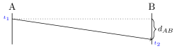
Figure 1: Simple ToA scheme

III-B Two-Way-Ranging

A first simple solution to compensate the missing synchronization between devices is the concept of Two Way Ranging (TWR) as determined in IEEE802.15.4 described in [13]. TWR systems include two devices $A$ and $B$, that are communicating bi-directional to measure a round-trip-time. This concept is simply described by $A$ sending a message at $t_{1}$ to $B$ (received at $t_{2}$) which gets then acknowledged after a fixed and known delay at time $t_{3}$ (sent from $B$). That acknowledgment arrives back at device $A$ at $t_{4}$. According to [13], $A$ can now calculate the ToF as follows:

$$d_{AB}=\frac{1}{2}\cdot(R_{A}-D_{B})$$ (3)

with $R_{A}:=t_{4}-t_{1}$ and $D_{B}:=t_{3}-t_{2}$ (comp. Fig. 2)

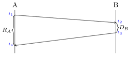
Figure 2: Simple TWR scheme

This method is expected to be better conditioned since we do not rely on the clocks being synchronized at the beginning of the measurement. Therefore the error should not accumulate in the same way as in simple ToA (Section III-A). This intuition is now substantiated. Similar as in Section (II-A) we define an erroneous model for the here relevant values:

$$\hat{R}_{A} :=R_{A}\cdot(1+\epsilon_{A})$$ (4)

$$\hat{D}_{B} :=D_{B}\cdot(1+\epsilon_{B})$$ (5)

And by using (3) we can define:

$$\hat{d}_{AB} :=\frac{1}{2}(\hat{R}_{A}-\hat{D}_{B})$$

$$=\frac{1}{2}\Big{[}(\hat{t}_{4}-\hat{t}_{1})-(\hat{t}_{3}-\hat{t}_{2})\Big{]}$$

$$\hat{\overline{AB}} :=c\cdot\hat{d}_{AB}$$

Again the difference between erroneous and error-free value states the error.

$$\tilde{\overline{AB}} =\hat{\overline{AB}}-\overline{AB}$$

$$=c\cdot\frac{1}{2}(\hat{R}_{A}-R_{A}-\hat{D}_{B}+D_{B})$$

$$=c\cdot\frac{1}{2}(\epsilon_{A}R_{A}-\epsilon_{B}D_{B})\text{ by using \eqref{eqn:simple_twr_ra} and \eqref{eqn:simple_twr_db}}$$

Using the fact that $R_{A}=D_{B}+2d_{AB}$ it follows:

$$=c\cdot\frac{1}{2}\Big{[}\epsilon_{A}(D_{B}+2d_{AB})-\epsilon_{B}D_{B}\Big{]}$$

$$=c\cdot\frac{1}{2}\Big{[}(\epsilon_{A}-\epsilon_{B})D_{B}+\epsilon_{A}2d_{AB}\Big{]}$$

And since $D_{B}\gg d_{AB}$ in realistic scenarios, we get the approximation:

$$\approx c\cdot\frac{1}{2}(\epsilon_{A}-\epsilon_{B})\cdot D_{B}$$

With clock-drift-error the worst value $(\epsilon_{A}-\epsilon_{B})$ can take on is $\frac{40}{1000000}$, so the worst case error introduced can be calculated as:

$$$3\text{\times}{10}^{8}$\frac{\text{m}}{\text{s}}\cdot\frac{1}{2}\cdot\frac{40}{1000000}\cdot D_{B}=$6\text{\times}{10}^{3}$\text{m}\cdot D_{B}$$

We observe that the clock error is only affecting the measurement during $D_{B}$ (on both clocks) and does not accumulate over the whole operation time. Nevertheless, we still consider the system too error prone in most cases since even a $D_{B}$ of one millisecond causes already six meters of error. A similar analysis is shown in [11, D1.3.1].

III-C Double-Sided Two-Way-Ranging

III-C1 Concept

To reduce the influence of drift-error in TWR, a new method called Double Sided Two Way Ranging (DS-TWR) is proposed. This method is described and defined in the IEEE 802.15.4 standard [11, D1.3.2]. They suggested adding a third message to the scheme as depicted in Fig. 3. Using this method the $d_{AB}$ respectively $\overline{AB}$ can (in the ideal case) be calculated as follows from Hach [3]:

$$d_{AB}=\frac{1}{4}(R_{A}-D_{B}+R_{B}-D_{A})$$ (6)

$$\overline{AB}=c\cdot d_{AB}$$ (7)

Similar to the previous method we can also calculate the error margin. First, we create a clock error model for this method like in (II-A):

$$\begin{array}[]{ccl}\hat{R}_{A}:=R_{A}\cdot(1+\epsilon_{A})\\ \hat{D}_{A}:=D_{A}\cdot(1+\epsilon_{A})\\ \hat{R}_{B}:=R_{B}\cdot(1+\epsilon_{B})\\ \hat{D}_{B}:=D_{B}\cdot(1+\epsilon_{B})\end{array}$$ (8)

And by using (6) and (7) we derive:

$$\hat{d}_{AB} :=\frac{1}{4}(\hat{R}_{A}-\hat{D}_{B}+\hat{R}_{B}-\hat{D}_{A})$$

$$\hat{\overline{AB}} :=c\cdot\hat{d}_{AB}$$

Again the difference between erroneous and error-free value states the error.

$$\tilde{\overline{AB}} =\hat{\overline{AB}}-\overline{AB}$$

$$=c\cdot\frac{1}{4}\Big{[}(R_{A}-D_{A})\cdot\epsilon_{A}+(R_{B}-D_{B})\cdot\epsilon_{B}\Big{]}$$

We then add and subtract to the inner brackets $D_{B}$ respectively $D_{A}$:

$$= \;c\cdot\frac{1}{4}\Big{[}(R_{A}-D_{B}+D_{B}-D_{A})\cdot\epsilon_{A}$$

$$+(R_{B}-D_{A}+D_{A}-D_{B})\cdot\epsilon_{B}\Big{]}$$

$$= \;c\cdot\frac{1}{4}\Big{[}(R_{A}-D_{B})\cdot\epsilon_{A}+(D_{B}-D_{A})\cdot\epsilon_{A}$$

$$+(R_{B}-D_{A})\cdot\epsilon_{B}+(D_{A}-D_{B})\cdot\epsilon_{B}\Big{]}$$

And since $2d_{AB}=R_{A}-D_{B}$ as well as $2d_{AB}=R_{B}-D_{A}$ we can substitute those:

$$=c\cdot\frac{1}{4}\Big{[}2d_{AB}\cdot(\epsilon_{A}+\epsilon_{B})+(D_{B}-D_{A})\cdot(\epsilon_{A}-\epsilon_{B})\Big{]}$$

$$=c\cdot\frac{1}{4}\Big{[}(D_{B}-D_{A})\cdot(\epsilon_{A}-\epsilon_{B})\Big{]}+c\cdot\frac{1}{4}\Big{[}2d_{AB}\cdot(\epsilon_{A}+\epsilon_{B})\Big{]}$$

$d_{AB}$ is in order of magnitude of nanoseconds and multiplied with a $\approx 20$ppm value, so it follows that the second term is in sub-picosecond order of magnitude. Even under multiplication with the large value of $c$, this would leave that part of the term as not significant for our accuracy requirements. Therefore only the first part of the term is relevant to us:

$$\approx c\cdot\frac{1}{4}(D_{B}-D_{A})\cdot(\epsilon_{A}-\epsilon_{B})$$

Again assuming $\pm 20$ppm as drift error (comp. Section II-A), the worst case value can then be calculated:

$$$3\text{\times}{10}^{8}$\frac{\text{m}}{\text{s}}\cdot\frac{1}{4}(D_{B}-D_{A})\cdot\frac{40}{1000000}=$3\text{\times}{10}^{3}$\text{m}\cdot(D_{B}-D_{A})$$

Where $(\epsilon_{A}-\epsilon_{B})$ can take on the value $\frac{40}{1000000}$ in the worst case. So as long as the difference $|D_{A}-D_{B}|$ is relatively small, we can assume a very low error.

In the following, we denote this method as Symmetrical Double Sided Two Way Ranging (SDS-TWR). With this method, it is at least in theory, possible to eliminate the drift error completely by selecting $D_{A}$ and $D_{B}$ to be identical. However, this is, in reality not possible (e.g. due to inaccuracy of scheduling sending time). To remove this requirement, the asymmetric approach was developed.

Figure 3: Double-Sided TWR scheme

III-C2 Asymmetric Formula

Keeping the difference $|D_{A}-D_{B}|$ small is not always possible or desired (for instance through technical limitations of the measuring/processing device). To address those restrictions, Neirynck et al. [8] developed a different (asymmetric) formula for the same scheme:

$$d_{AB}: =\frac{R_{A}R_{B}-D_{A}D_{B}}{2(R_{A}+D_{A})}$$ (9)

$$=\frac{R_{A}R_{B}-D_{A}D_{B}}{2(R_{B}+D_{B})}$$ (10)

$$\overline{AB} :=c\cdot d_{AB}$$ (11)

$\Rightarrow$ Using $D_{B}+R_{B}=R_{A}+D_{A}$ (comp. Fig. 3)

$$d_{AB}=\frac{R_{A}R_{B}-D_{A}D_{B}}{R_{A}+R_{B}+D_{A}+D_{B}}$$ (12)

When this adjusted formula is applied, we refer to the method as Asymetric Double Sided Two Way Ranging (asym-DS-TWR). The formula is in the following proven to be more resilient to differences between $D_{A}$ and $D_{B}$.

Using the same clock error model as for the symmetric solution (8) and applying it to (9) we define:

$$\hat{d}_{AB} :=\frac{\hat{R}_{A}\hat{R}_{B}-\hat{D}_{A}\hat{D}_{B}}{2(\hat{R}_{A}+\hat{D}_{A})}$$

$$=\frac{(1+\epsilon_{A})(1+\epsilon_{B})}{(1+\epsilon_{A})}\cdot\frac{R_{A}R_{B}-D_{A}D_{B}}{R_{A}+D_{A}}$$

And equivalently using (10) we derive:

$$=\frac{\hat{R}_{A}\hat{R}_{B}-\hat{D}_{A}\hat{D}_{B}}{2(\hat{R}_{B}+\hat{D}_{B})}$$

$$=\frac{(1+\epsilon_{A})(1+\epsilon_{B})}{(1+\epsilon_{B})}\cdot\frac{R_{A}R_{B}-D_{A}D_{B}}{R_{B}+D_{B}}$$

With (11) it follows the definition:

$$\hat{\overline{AB}}:=c\cdot\hat{d}_{AB}$$ (13)

The difference between erroneous and error-free value states the absolute error.

$$\tilde{\overline{AB}} =\hat{\overline{AB}}-\overline{AB}$$

$$=c\cdot\epsilon_{A}d_{AB}\text{ using \eqref{eqn:asym_ds_twr_eqn_a}}$$

and

$$=c\cdot\epsilon_{B}d_{AB}\text{ using \eqref{eqn:asym_ds_twr_eqn_b}}$$

Like in (12) we can combine those:

$$\hat{\overline{AB}} =c\cdot\Big{[}\frac{1}{2}(\epsilon_{A}+\epsilon_{B})\cdot d_{AB}\Big{]}$$

$$=\frac{\epsilon_{A}+\epsilon_{B}}{2}\cdot\overline{AB}$$

So in the worst case we can assume to have an error of $\frac{20}{1000000}\cdot\overline{AB}$ which is non-significant in almost all cases. This is achieved without having similar $D_{A}$ and $D_{B}$. It is important to note that we assumed a constant clock drift during the time of measurement in our clock-model (II-A) .

IV Time Difference of Arrival

Beside the ToA methods described there is the group of TDoA-based methods.

In contrast to ToA, TDoA methods have less strict device capability requirements. For example, some of the following methods allow to position Tags which are not actively responding in reaction to the Anchors’ signals, while some methods allow the Anchor network to stay silent (no transmission) during positioning. A few beneficial features resulting from that are for instance the possibility to increase the number of Nodes that are simultaneously positioned or the ability to position devices without their knowledge or devices which are incapable of measuring time.

The difference between ToA and TDoA becomes clear when looking at an example for a simplified version of a TDoA method.

IV-A Simple TDoA

Simple-TDoA is a method in which we do not measure the ToF between two devices. Instead, we measure the difference in distances/time between each of two devices $X$ and $Z$ to one device $Y$ (comp. Fig. 4). This value is called a Time-Difference-of-Arrival- or short TDoA-value and is in this document denoted as $T_{XZ}^{Y}$.

The mathematical definition of this TDoA value is:

$$T_{XZ}^{Y}:=d_{YZ}-d_{YX}$$

Figure 4: TDoA value graphically

The simplest setup in which we would effectively gather that value would consist of three perfectly synchronized and drift-free devices $A,B,S$ from which $S$ transmits a message at a time $t_{1}$, and the signal arrives at $A$ at time $t_{1}$, and at $B$ at time $t_{2}$ as depicted in Fig. 5

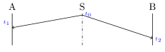
Figure 5: Simple TDoA

We can then calculate:

$$T_{AB}^{S}=t_{2}-t_{1}$$ (14)

The transmitting device $S$ is here interpreted as Tag while $A$ and $B$ are operating as Anchors. Multiple such measurements on additional Anchor devices (with known positions), in relation to the same Tag, would allow to apply hyperbolic solver algorithms like Chan and Ho [2] to determine the Tags position.

When calculating the error of this setup we have to assume that since the last perfect synchronization ($t=0$), drift effects have been accumulated by the individual clocks.

As with ToA methods previously we now primarily define our erroneous model like in (II-A):

$$\hat{t}_{1} :=t_{1}\cdot(1+\epsilon_{A})$$

$$\hat{t}_{2} :=t_{2}\cdot(1+\epsilon_{B})$$

And using (14):

$$\hat{T}_{AB}^{S} :=\hat{t}_{2}-\hat{t}_{1}$$

Again the difference between erroneous and error-free value states the error.

$$\tilde{T}_{AB}^{S} =\hat{T}_{AB}^{S}-T_{AB}^{S}$$

$$=\epsilon_{B}t_{2}-\epsilon_{A}t_{1}$$

Using the fact that $t_{2}=t_{1}+T_{AB}^{S}$ we can write

$$=\epsilon_{B}(t_{1}+T_{AB}^{S})-\epsilon_{A}t_{1}$$

$$=t_{1}(\epsilon_{B}-\epsilon_{A})+\epsilon_{B}T_{AB}^{S}$$

And since $T_{AB}^{S}$ is in order of magnitude of nanoseconds and is multiplied with a $\approx 20$ppm value the second part of the term is in sub-picosecond order of magnitude. Therefore only the first part of the term appears to be relevant, and we can approximate it with:

$$t_{1}\cdot(\epsilon_{B}-\epsilon_{A})$$ (15)

That means that we have to assume a worst-case error of $\approx\frac{40}{1000000}\cdot t_{1}$. Which makes the method already after a short time of operation unusable for realistic scenarios.

IV-B Whistle

To resolve that issue of fast degrading synchronization. Xu et al. [5] proposed a method called Whistle. Whistle tries to reduce the timespan in which the synchronization drift can occur. That is achieved by adding another signal into the simple TDoA scheme as shown in Fig. 6

Figure 6: Whistle

This additional message exchange between $A$ and $B$ can be interpreted as a form of “resynchronization” between both devices. According to Xu et al. [5] the TDoA value between those devices can now be calculated by:

$$T_{AB}^{S} :=d_{AB}-(t_{4}-t_{1})+(t_{3}-t_{2})$$

$$=d_{AB}-R_{A}+D_{B}$$ (16)

The Anchor that is replying (here $B$) is called Mirror. Note that we require that the distance between the Mirror and the other Anchor devices is known.

Now we calculate the error resulting from this improved protocol. First, we define the erroneous model like in (II-A):

$$\hat{R}_{A} :=R_{A}\cdot(1+\epsilon_{A})$$

$$\hat{D}_{B} :=D_{B}\cdot(1+\epsilon_{B})$$

Then using (16):

$$\hat{T}_{AB}^{S} :=d_{AB}-\hat{R}_{A}+\hat{D}_{B}$$

Again the difference between erroneous and error-free value states the error.

$$\tilde{T}_{AB}^{S} :=\hat{T}_{AB}^{S}-T_{AB}^{S}$$

$$=\epsilon_{B}D_{B}-\epsilon_{A}R_{A}$$

And using the fact that $R_{A}=D_{B}+d_{AB}+T_{AB}^{S}$ it follows:

$$=\epsilon_{B}D_{B}-\epsilon_{A}(D_{B}+d_{AB}+T_{AB}^{S})$$

$$=\epsilon_{A}(d_{AB}+T_{AB}^{S})+D_{B}(\epsilon_{B}-\epsilon_{A})$$

$d_{AB}$ and $T_{AB}^{S}$ are in order of magnitude of nanoseconds. And since those are multiplied with a $\approx 20$ppm value in the first part of the term, that part of the term is in sub-picosecond order of magnitude. Therefore only the second part of the term is relevant.

$$\approx D_{B}(\epsilon_{B}-\epsilon_{A})$$ (17)

Assuming the same realistic worst case drift values as previously we end up with a worst-case error estimate of $D_{B}\cdot\frac{40}{1000000}$. This is an improvement compared to the simple TDoA method since the error is not dependent on synchronized clocks and is therefore also not accumulating. On the other hand, a typical value for $D_{B}$ is one millisecond which leads already to $40$ nanoseconds $\approx 12$ meters of error. This approach is therefore not practically usable with radio platforms that operate with industry standard clocks.

IV-C Djaja-Josko-Kolakowski Method

A method combining the benefits of SDS-TWR and Whistle was proposed by Djaja-Josko and Kolakowski [7], and therefore we refer to it as Djaja-Josko-Kolakowski-Method (DJKM).

The essential idea of DJKM is to execute an optimized version of SDS-TWR in a group of Anchor devices. While doing so, it is possible for eavesdropping Tags to collect TDoA information to those Anchors. To simplify the explanation of the method the sequence diagram Fig. 7 was reduced to two Anchors (one of them could be interpreted as “acting Mirror”) and a single Tag. For details about the interaction between more than two Anchors we refer to the original paper [7].

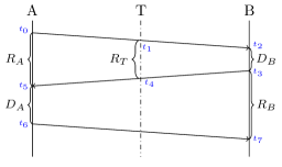
Figure 7: Djaja-Josko-Kolakowski Method

The authors derived the following formula to calculate the TDoA values:

$$T_{AB}^{T} =(t_{4}-t_{1})-(t_{3}-t_{2})-d_{AB}$$

$$=R_{T}-D_{B}-d_{AB}$$ (18)

It is important to note that Tag $T$ is only in receiving mode which is an essential functional difference to Whistle where the Tag $S$ is at all times in transmit mode only. Moreover, when comparing DJKM s TDoA calculation with the one from Whistle (16) and comparing the modes of operation of Anchors and Tags between both method DJKM appears to us like an “inverse Whistle” method. Especially in Ultra Wide Band (UWB) it is common that transmission operations use significantly less energy than receiving (comp. [14, Sct 7.2]), so for battery driven Tag devices the Whistle approach is consuming less energy.

Now we demonstrate that the worst-case error for DJKM is identical to Whistle. Again we first define the erroneous model like in (II-A):

$$\hat{R}_{T} :=R_{T}\cdot(1+\epsilon_{T})$$

$$\hat{D}_{B} :=D_{B}\cdot(1+\epsilon_{B})$$

Using (18)

$$\hat{T}_{AB}^{T} :=\hat{R}_{T}-\hat{D}_{B}-d_{AB}$$

The difference between erroneous and error-free value states the error.

$$\tilde{T}_{AB}^{T} =\hat{T}_{AB}^{T}-T_{AB}^{T}$$

$$=\epsilon_{T}R_{T}-\epsilon_{B}D_{B}$$

Using the fact that $R_{T}=D_{B}+d_{AB}+T_{AB}^{T}$:

$$=\epsilon_{T}(D_{B}+d_{AB}+T_{AB}^{T})-\epsilon_{B}D_{B}$$

$$=\epsilon_{T}(d_{AB}+T_{AB}^{T})+(\epsilon_{T}-\epsilon_{B})D_{B}$$

For the same reason we described in Whistle (IV-B) we can neglect the first part as not significant and so approximate the term with.

$$\approx(\epsilon_{T}-\epsilon_{B})D_{B}$$ (19)

When choosing worst-case epsilons, we end up with the worst case estimate $D_{B}\cdot\frac{40}{1000000}$. That is identical to the estimate for Whistle.

Djaja-Josko and Kolakowski [7] also point out that their scheme simultaneously allows for the calculation of SDS-TWR values between certain Anchors in the ranging scheme.

IV-D Double-Pulsed-Whistle

We have shown that the TDoA values of DJKM have a similar error as Whistle. That means that all described methods of synchronization-free TDoA are still prone to clock-drift errors on a scale too large for most radio-based applications. To circumvent these problems with TDoA and to make the methods more applicable in practice a new approach was proposed by Tschirschnitz and Wagner [6]. This method called Double Pulsed Whistle (DPW) introduces a second pulse to the known Whistle scheme and uses symmetries to reduce the clock error significantly. The error reduction uses similar effects like the methods of DS-TWR. The transmission scheme is displayed in Fig. 8.

Table I: Comparison between the separate methods

	Clock-Drift induced Error	Anchor Nodes	Tag Nodes
Simple ToA ((III-A))	$t_{1}\cdot(\epsilon_{B}-\epsilon_{A})$	RX	TX
TWR (III-B)	$\frac{1}{2}(\epsilon_{A}-\epsilon_{B})\cdot D_{B}$	TX + RX	TX + RX
SDS-TWR (III-C)	$\frac{1}{4}(\epsilon_{A}-\epsilon_{B})\cdot(D_{B}-D_{A})$	TX + RX	TX + RX
Asym-DS-TWR (III-C2)	$\frac{1}{2}(\epsilon_{A}+\epsilon_{B})\cdot d_{AB}$	TX + RX	TX + RX
Simple TDOA (IV-A)	$(\epsilon_{B}-\epsilon_{A})\cdot t_{1}$	RX	TX
Whistle (IV-B)	$(\epsilon_{B}-\epsilon_{A})\cdot D_{B}$	RX + one TX	TX
DJKM (IV-C)	$(\epsilon_{T}-\epsilon_{B})\cdot D_{B}$	RX + TX	RX
DP-Whistle (IV-D)	$(\epsilon_{A}+\epsilon_{B})\cdot d_{AB}$	RX + one TX	TX

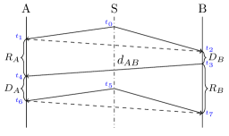
Figure 8: Double Pulsed Whistle

Using the findings from Tschirschnitz and Wagner [6] the TDoA value can then be calculated as follows:

$$T_{AB}^{S} :=\frac{R_{A}R_{B}-D_{A}D_{B}}{R_{A}+D_{A}}-d_{AB}$$ (20)

$$=\frac{R_{A}R_{B}-D_{A}D_{B}}{R_{B}+D_{B}}-d_{AB}$$ (21)

Using $R_{A}+D_{A}=R_{B}+D_{B}$ we conclude:

$$T_{AB}^{S}=\frac{2(R_{A}R_{B}-D_{A}D_{B})}{R_{A}+R_{B}+D_{A}+D_{B}}-d_{AB}$$ (22)

Again we use the same erroneous clock model as in (8) conforming to our model design in (II-A) to define the erronous timespans ($\hat{R}_{A},\hat{D}_{A},\hat{R}_{B},\hat{D}_{B}$). Then applying it to (20) we define:

$$\hat{T}_{AB}^{S} :=\frac{\hat{R}_{A}\hat{R}_{B}-\hat{D}_{A}\hat{D}_{B}}{\hat{R}_{A}+\hat{D}_{A}}-d_{AB}$$

And equivalently using (21) we derive:

$$=\frac{\hat{R}_{A}\hat{R}_{B}-\hat{D}_{A}\hat{D}_{B}}{\hat{R}_{B}+\hat{D}_{B}}-d_{AB}$$

We transform the term with denominator $\hat{R}_{B}+\hat{D}_{B}$:

$$\hat{T}_{AB}^{S} =\frac{(1+\epsilon_{A})(1+\epsilon_{B})}{(1+\epsilon_{B})}\cdot\frac{R_{A}R_{B}-D_{A}D_{B}}{R_{A}+D_{A}}-d_{AB}$$

Adding and subtracting $(1+\epsilon_{A})d_{AB}$ to the term brings:

$$= \;(1+\epsilon_{A})\cdot\frac{R_{A}R_{B}-D_{A}D_{B}}{R_{A}+D_{A}}$$

$$-(1+\epsilon_{A})d_{AB}+(1+\epsilon_{A})d_{AB}-d_{AB}$$

Then substituting with (20) delivers:

$$=(1+\epsilon_{A})\cdot T_{AB}^{S}+(1+\epsilon_{A})d_{AB}-d_{AB}$$

$$=(1+\epsilon_{A})\cdot T_{AB}^{S}+\epsilon_{A}d_{AB}$$

The difference between the erroneous and error-free value is the error:

$$\tilde{T}_{AB}^{S} :=\hat{T}_{AB}^{S}-T_{AB}^{S}$$

$$=\epsilon_{A}T_{AB}^{S}+\epsilon_{A}d_{AB}$$

$$\leq 2\epsilon_{A}d_{AB}$$

The fact that $T_{AB}^{S}\leq d_{AB}$ justifies the last step here. That is true since the TDoA ($T_{AB}^{S}$) can never grow larger than the distance between the measuring Anchor pair ($d_{AB}$).

Equivalently we can apply this to the term with the divisor $\hat{R}_{B}+\hat{D}_{B}$:

$$\hat{T}_{AB}^{S} =\frac{(1+\epsilon_{A})(1+\epsilon_{B})}{(1+\epsilon_{A})}\cdot\frac{R_{A}R_{B}-D_{A}D_{B}}{R_{A}+D_{A}}-d_{AB}$$

$$=(1+\epsilon_{B})\cdot T_{AB}^{S}+\epsilon_{B}d_{AB}$$

$$\tilde{T}_{AB}^{S} =\epsilon_{B}T_{AB}^{S}+\epsilon_{B}d_{AB}$$

$$\approx 2\epsilon_{B}d_{AB}$$

Combining the two fraction like in (22) we end up with:

$$\tilde{T}_{AB}^{S}\approx(\epsilon_{A}+\epsilon_{B})d_{AB}$$ (23)

We observe that the error is now only depending on the distance value $d_{AB}$ which is in order of nanoseconds for typical positioning setups. We further multiply it with $\epsilon$’s which are in magnitudes of $\pm 20$ppm. That means that the error is in no significant magnitudes.

V Summary and Conclusion

In the Table I all of the methods described in this paper are listed. Their worst-case clock-error and the required device capabilities for Anchors and Tags are listed for each method. For better comparison of the worst-case clock-drift errors the methods are divided into ToA and TDoA methods. On the right, the interface requirements for Anchor- and Tag-Nodes are noted for each method.

The table reiterates that all methods which use double-pulses like DPW and asym-DS-TWR are much more robust against clock errors. Especially for radio based ToF methods like UWB it is important to reduce these error sources because the contributions of the clock error in Whistle and DJKM could significantly distort the result.

In future work, approaches like DJKM can be extended to incorporate the Double-Pulse similar to the transition from Whistle to DPW. This would keep the advantages of DJKM like allowing unlimited number of Tags with the advantages of high robustness against clock errors.

This approach is related to our efforts in designing Double Pulsed Positioning [15] a novel infrastructure-less and synchronisation-free ToF method.

References

- Murphy and Hereman [1995] W. Murphy and W. Hereman, “Determination of a position in three dimensions using trilateration and approximate distances,” Department of Mathematical and Computer Sciences, Colorado School of Mines, Golden, Colorado, MCS-95, vol. 7, p. 19, 1995.
- Chan and Ho [1994] Y. T. Chan and K. C. Ho, “A simple and efficient estimator for hyperbolic location,” IEEE Transactions on Signal Processing, vol. 42, no. 8, pp. 1905–1915, 8 1994.
- Hach [2005] R. Hach, “Symmetric double side two way ranging,” IEEE 802.15 WPAN Documents, 15-05-0334-r00, 2005.
- Sahinoglu and Gezici [2006] Z. Sahinoglu and S. Gezici, “Ranging in the ieee 802.15.4a standard,” in 2006 IEEE Annual Wireless and Microwave Technology Conference, 12 2006, pp. 1–5.
- Xu et al. [2011] B. Xu, R. Yu, G. Sun, and Z. Yang, “Whistle: Synchronization-free tdoa for localization,” in 2011 31st International Conference on Distributed Computing Systems, 6 2011, pp. 760–769.
- Tschirschnitz and Wagner [2018] M. V. Tschirschnitz and M. Wagner, “Synchronization-free and low power tdoa for radio based indoor positioning,” in 2018 International Conference on Indoor Positioning and Indoor Navigation (IPIN), 9 2018, pp. 1–4.