SPSC: a new execution policy for exploring discrete-time stochastic simulations

Abstract

In this paper, we introduce a new method called SPSC (Simulation, Partitioning, Selection, Cloning) to estimate efficiently the probability of possible solutions in stochastic simulations. This method can be applied to any type of simulation, however it is particularly suitable for multi-agent-based simulations (MABS). Therefore, its performance is evaluated on a well-known MABS and compared to the classical approach, i.e., Monte Carlo.

1 Introduction

Multi-agent-based simulations (MABS) are widely used in various fields to study complex systems [6]. Most of them are combined with stochasticity to represent non fully controllable phenomena and use a discrete-time approach to facilitate model construction. Such model can generally be described as taking some initial conditions and some parameter set as inputs, in order to return outputs at each time step (c.f. Figure 1).

Before running into exploration of the parameter set or the initial condition space, we must first analyze outcomes from a fixed parameter set and initial conditions. Let us denote a stochastic simulation outputs (called observables in the following) at a final time step $T$ as a random vector $\boldsymbol{X}_{T}$. Then a key question to address is: what is the probability $\mathbb{P}(\boldsymbol{X}_{T}\in\mathcal{S})=\theta_{\mathcal{S}}$ of a specific solution $\mathcal{S}$?

Figure 1: Illustration of a discrete-time stochastic simulation

The classical method to handle this question is Monte Carlo simulation (MC) [7]. It consists in simulating a number $n$ of replications and building an estimator $\hat{\theta}_{\mathcal{S}}$ of $\theta_{\mathcal{S}}$ defined as:

$$\hat{\theta}_{\mathcal{S}}=\frac{1}{n}\sum_{i=1}^{n}\mathds{1}_{\mathcal{S}}(\boldsymbol{X}_{T}^{i})$$ (1)

where $\mathds{1}_{\mathcal{S}}$ is the indicator function of the set $\mathcal{S}$ and $\boldsymbol{X}_{T}^{i}$ the value of observables in the $i^{\text{th}}$ replication. The issue with this approach is that for the estimator to be good, the number $n$ has generally to be large, as illustrated in Section 2.

Some methods have been developed to speed-up the computation of such simulations, such as splitting [3] or polyagent [5]. However, they look for specific solutions (rare or mean), assume a particular modeling approach (Markov chains or agent-based) and require some low-level manipulations of the model.

In this paper, we propose a policy that simulates an authorized number $N$ of replications and is as generic as the MC approach yet provides a better estimator when computational resources are limited (i.e. small $N$).

The paper is organized as follows: Section 2 recalls and illustrates a standard approach to determine the required number of replications in Monte Carlo simulation for a single observable. The design principles and the approach proposed to answer the above-mentioned issues are presented in Section 3 and then applied to a classical MABS in Section 4. Section 5 concludes the paper.

2 Monte Carlo simulation, how many replications?

We recall in this section a standard approach to determine the number $n(X_{T,i})$ of replications to obtain a good estimator $\hat{\theta}_{S_{i}}$ of the probability $\mathbb{P}(X_{T,i}\in S_{i})=\theta_{S_{i}}$ of some solution $S_{i}$ where $X_{T,i}$ is one observable of the vector $\boldsymbol{X}_{T}$. Suppose a desired relative error $\epsilon$ for the estimator $\hat{\theta}_{S_{i}}$ at confidence level $1-\alpha$ :

$$\mathbb{P}(\frac{|\hat{\theta}_{S_{i}}-{\theta}_{S_{i}}|}{{\theta}_{S_{i}}}\leq\epsilon)\geq 1-\alpha.$$ (2)

The minimal value for $n(X_{T,i})$ to verify (2) can be determined by applying the following algorithm [1, p. 449]:

1. Simulate $n_{0}$ replications. ($n_{0}$ observations $X_{T,i}^{1},\dots,X_{T,i}^{n_{0}}$)

2. Compute

   $$n(X_{T,i})=\lceil(\frac{Z_{1-(\frac{\alpha}{2})}\cdot s_{i}}{\epsilon\cdot\overline{X}_{T,i}})^{2}\rceil$$ (3)

   where $Z_{1-(\alpha/2)}$ is the $100(1-\alpha/2)$ quantile of the normal distribution, $s_{i}$ stands for the sample standard deviation over the $n_{0}$ observations and $\overline{X}_{T,i}$ is the sample mean value over the $n_{0}$ observations. The conventional values for $n_{0}$, $\epsilon$ and $\alpha$ are respectively $150$, $0.05$ and $0.05$.

Afterward, we can then deduce the necessary number $n$ satisfying every observable as:

$$n=\max_{X_{T,i}\in\boldsymbol{X_{T}}}n(X_{T,i})$$ (4)

To illustrate this algorithm, let us take an academic example. We consider an environment containing vegetation and 2 types of agents: preys consuming the vegetation and predators hunting preys for food. Both preys and predators can move without restriction in the environment. This model has been implemented on the Similar platform [4] and is based on the NetLogo wolf sheep predation model [8]. The set of observables here consists of the populations of different species at each time step. The necessary number $n$ for some arbitrarily chosen parameter set and initial state of the simulation, using the conventional values for $n_{0}$, $\epsilon$ and $\alpha$, is 3600 (c.f. Table 1). However, if we want a more precise estimation, the necessary number $n$ of replications increases drastically: for example, considering a relative error $\epsilon=0.005$ yields a necessary number of replications $n=7249285$.

Table 1: Determination of the necessary number of replications for the prey predator model implemented on the Similar platform. The parameters applied are $n_{0}=150$, $\epsilon=0.05$ and $\alpha=0.05$.

$X_{T,i}$	$s_{i}$	$\overline{X}_{T,i}$	$n(X_{T,i})$
number of preys	697.83	783.77	1219
number of predators	196.95	128.67	3600

3 A new execution policy for stochastic simulations

In this section, we introduce a new execution policy for stochastic simulations called SPSC (Simulation, Partitioning, Selection, Cloning). This approach relies on a decomposition of the probability of interest that we explain first.

3.1 Decomposition of the probability of interest

The probability $\mathbb{P}(\boldsymbol{X}_{T}\in\mathcal{S})$ concerns the observables with respect to a specific solution $\mathcal{S}$ at some final time step $T$. Thanks to the law of total probability, considering some intermediate time step $j$ before $T$, we can write

$$\mathbb{P}(\boldsymbol{X}_{T}\in\mathcal{S})=\sum_{\mathcal{S}_{j}\in\mathscr{P}_{j}}\mathbb{P}(\boldsymbol{X}_{T}\in\mathcal{S}|\boldsymbol{X}_{j}\in\mathcal{S}_{j})\mathbb{P}(\boldsymbol{X}_{j}\in\mathcal{S}_{j})$$ (5)

where $\mathscr{P}_{j}$ is a partition of the state space of the random vector $\boldsymbol{X}_{j}$.

More generally, considering all time steps before $T$, we can obtain the following decomposition by assuming a discrete-time system where $\boldsymbol{X}_{i}$ depends only on $\boldsymbol{X}_{i-1}$:

$$\mathbb{P}(\boldsymbol{X}_{T}\in\mathcal{S})=\sum_{\begin{subarray}{c}\mathcal{S}_{T-1}\in\mathscr{P}_{T-1}\\ \vdots\\ \mathcal{S}_{1}\in\mathscr{P}_{1}\end{subarray}}\prod_{i=0}^{T-1}\mathbb{P}(\boldsymbol{X}_{i+1}\in\mathcal{S}_{i+1}|\boldsymbol{X}_{i}\in\mathcal{S}_{i})$$ (6)

where $\mathscr{P}_{i}$, $i=1,...,T-1$, is a partition of the state space of $\boldsymbol{X}_{i}$, $\mathcal{S}_{T}=\mathcal{S}$ and $\mathcal{S}_{0}$ is the initial state of the simulation.

3.2 SPSC: Simulation, Partitioning, Selection, Cloning

Inspired by the decomposition (6), we split the time interval $[0,T]$ into $m$ pieces: $[t_{(0)},t_{(1)}],[t_{(1)},t_{(2)}],...,[t_{(m-1)},t_{(m)}]$ where $t_{(0)}=0<t_{(1)}<...<t_{(m-1)}<t_{(m)}=T$. Then, for each interval $[t_{(i)},t_{(i+1)}]$ the following steps are applied (c.f. Figures 2 and 3):

Simulation

Simulate $N$ replications from $t_{(i)}$ to $t_{(i+1)}$, $i\in\{0,\ldots,m-1\}$, where $N$ corresponds to the number of replications we authorize for the simulation.

Partitioning

At time $t_{(i+1)}$, form a partition of the space of observables of these $N$ replications. This can be done by applying a clustering algorithm.

Selection

Choose one or multiple representative replications (which we call delegates) from each partition and discard the other replications.

Cloning

Clone the selected delegates to obtain $N$ replications in total.

Figure 2: SPSC process diagram

Once the iterations are finished, we have created for each $t_{(i)}$ a partition $\mathscr{P}_{(i)}$ for the state space of $\boldsymbol{X}_{t_{(i)}}$. For an element $\mathcal{S}_{(i)}\in\mathscr{P}_{(i)}$ of the partition at time step $t_{(i)}$, after the selection and cloning steps, it has $n_{i}$ cloned replications. Besides, among these $n_{i}$ cloned replications, after evolving to the next time step $t_{(i+1)}$, some of them ($n_{i+1}$ replications) belong to some element $\mathcal{S}_{(i+1)}\in\mathscr{P}_{(i+1)}$. We propose to use the numbers $n_{i}$ and $n_{i+1}$ to approximate the conditional probability $\mathbb{P}(\boldsymbol{X}_{t_{(i+1)}}\in\mathcal{S}_{(i+1)}|\boldsymbol{X}_{t_{(i)}}\in\mathcal{S}_{(i)})$ by:

$$\hat{P}(\boldsymbol{X}_{t_{(i+1)}}\in\mathcal{S}_{(i+1)}|\boldsymbol{X}_{t_{(i)}}\in\mathcal{S}_{(i)})=\frac{n_{i+1}}{n_{i}}$$ (7)

Finally, we define an estimator $\hat{\theta}_{\mathcal{S}}$ for $\mathbb{P}(\boldsymbol{X}_{T}\in\mathcal{S})$ using a similar decomposition as that of Equation (6), based on time steps $t_{(i)}$ and (7):

$$\hat{\theta}_{\mathcal{S}}=\sum_{\begin{subarray}{c}\mathcal{S}_{(m-1)}\in\mathscr{P}_{(m-1)}\\ \vdots\\ \mathcal{S}_{(1)}\in\mathscr{P}_{(1)}\end{subarray}}\prod_{i=0}^{m-1}\hat{P}(\boldsymbol{X}_{t_{(i+1)}}\in\mathcal{S}_{(i+1)}|\boldsymbol{X}_{t_{(i)}}\in\mathcal{S}_{(i)})$$ (8)

where $\mathcal{S}_{(m)}=\mathcal{S}$ and $\mathcal{S}_{(0)}=\mathcal{S}_{0}$.

Figure 3: Illustration of the first and second iterations of SPSC, starting from a single initial state.

3.3 Implementation

We describe here a simple implementation of SPSC used in the experiment in Section 4:

Simulation

No special action is taken in this step.

Partitioning

$N$ replications provide $N$ instances of observables. To form a partition in the space of observables, we can take advantage of existing unsupervised learning algorithm which can separate instances by multiple subgroups. The well-known clustering process kmeans has been chosen to fulfill the task. The number of cluster $k$ is preset to 15.

Selection

From any element $\mathcal{S}_{(i)}\in\mathscr{P}_{(i)}$ of an intermediate partition, we select the replication which is the nearest to the center using euclidean distance on the space of observables.

Cloning

After partitioning and selection, $k$ delegates are obtained to be cloned. To come back to $N$ replications in total, we clone each delegate $\lfloor\frac{N}{k}\rfloor$ times. If $k$ does not divide $N$, we select randomly the remainder number $N-k*\lfloor\frac{N}{k}\rfloor$ of delegates to produce one more clone per selected delegate.

The time interval $[0,T]$ is homogeneously split into $m=5$ pieces (i.e. $\forall i\in\{0,1,\dots,5\}$, $t_{(i)}=i\times\frac{T}{5}$).

4 Experiment

Let us take the prey predator model mentioned previously in Section 2 as an example. As this model is well-known and well-studied, we can give some possible solutions before launching simulations:

$\mathcal{S}_{1}$:

Extinction of preys and predators, only vegetation remains.

$\mathcal{S}_{2}$:

Predators go extinct, preys live without nature enemy’s harass.

$\mathcal{S}_{3}$:

All species survive and form a stable ecosystem.

Now the question is, for an arbitrary parameter set and initial condition, what is the probability of these solutions at a given time step (e.g. $T=1000$)? To answer this question, the MC approach recalled in Section 2 is generally used.

In the following, we compare the performances of MC and SPSC. The validation is done by comparing the outputs of these methods with the same limited number of replications $N=50$. By repeating the simulations 1000 times, we will be able to compare statistically the results obtained by MC and SPSC. Two performance measures are considered here : 1)  The detection rate of a specific solution $\mathcal{S}$. 2) The precision of the probability estimator for a specific solution. Before evaluating these performance measures, we have done 30000 replications using MC in order to provide reference values for the comparisons:

$$P_{ref}(\mathcal{S}_{1})\approx 0.0065,P_{ref}(\mathcal{S}_{2})\approx 0.0126,P_{ref}(\mathcal{S}_{3})\approx 0.981$$ (9)

The detection rates obtained with MC and SPSC policies, i.e, the capacity of identifying a specific solution, from N = 50 replications are summed up in Table 2. The first three columns indicate the detection rate of single solutions and the last column indicate the detection rate for the three solutions simultaneously. We can then deduce that SPSC explores more efficiently the solution space.

Table 2: Detection rates obtained with MC and SPSC when launching 50 replications.

	$\mathcal{S}_{1}$	$\mathcal{S}_{2}$	$\mathcal{S}_{3}$	$\mathcal{S}_{1}$, $\mathcal{S}_{2}$ and $\mathcal{S}_{3}$
MC	0.236	0.455	1	0.102
SPSC	0.332	0.617	1	0.203

To evaluate the precision of the probability estimator, the absolute error between the probability estimator outcomes and the references is computed:

$$Err(\mathcal{S}_{i})=|\hat{P}(\mathcal{S}_{i})-P_{ref}(\mathcal{S}_{i})|.$$ (10)

Furthermore, to gain an entire vision on the three solutions simultaneously, we consider also the mean of three solutions relative errors:

$$\overline{Err}=\sum_{1\leq i\leq 3}|\frac{\hat{P}(\mathcal{S}_{i})-P_{ref}(\mathcal{S}_{i})}{P_{ref}(\mathcal{S}_{i})}|.$$ (11)

Histograms of these errors for the policies SPSC and MC are shown in Fig. 4.

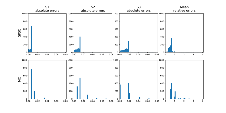
Figure 4: Comparison of errors

We can notice that the distribution of errors are not normal nor symmetric. Thus, to compare the errors from MC and SPSC policies, the Wilcoxon-Mann-Whitney test is applied with the threshold $\alpha=0.05$. The test results are presented in Table 3 with p-value and alternative hypotheses, we can then conclude that SPSC yields better probability estimates for each solution than MC.

Table 3: Hypothesis and p-value given by Wilcoxon-Mann-Whitney test.

Target solution	Alternative hypotheses	p-value	Conclusion
$\mathcal{S}_{1}$	$Err_{SPSC}<Err_{MC}$	2.2e-16	$Err_{SPSC}<Err_{MC}$
$\mathcal{S}_{2}$	$Err_{SPSC}<Err_{MC}$	3.163e-16	$Err_{SPSC}<Err_{MC}$
$\mathcal{S}_{3}$	$Err_{SPSC}<Err_{MC}$	9.849e-09	$Err_{SPSC}<Err_{MC}$
$\mathcal{S}_{1}$, $\mathcal{S}_{2}$ and $\mathcal{S}_{3}$	$\overline{Err}_{SPSC}<\overline{Err}_{MC}$	2.2e-16	$\overline{Err}_{SPSC}<\overline{Err}_{MC}$

5 Conclusions and perspectives

We have introduced a generic policy called SPSC for executing stochastic simulations that deals with the weakness of MC when the number of replications is limited. It treats simulations as black boxes and therefore, does not rely upon a priori knowledge. We have also presented a simple implementation of SPSC and run it on a classic stochastic MABS model. By comparing the results obtained with SPSC and with MC, we can conclude that SPSC gives a better solution probability estimation and can reveal more different solutions than MC.

The first perspectives of this work are related to the impact of the parameters ($N$, $k$, etc.), the partitioning algorithm as well as the selection and cloning strategies on the performance. For instance, instead of having the same number of clones for each delegate, we could clone more the delegates from small partitions and less the delegates from large partitions. Theoretical properties of the proposed solution as well as its interest for multimodal transport simulation will also be investigated.

Moreover, since we deal with small sample size at each intermediate time step, we could take advantage of modern tools [2] for statistical inference to compute the estimator $\hat{\theta}_{\mathcal{S}}$.

References

- [1] Banks, J., Carson II, J., Nelson, B., Nicol, D.: Discrete-event system simulation. Pearson, 5th edn. (2010)
- [2] Kanjanatarakul, O., Denœux, T., Sriboonchitta, S.: Prediction of future observations using belief functions: A likelihood-based approach. Int J Approx Reason 72, 71–94 (2016)
- [3] L’Ecuyer, P., Le Gland, F., Lezaud, P., Tuffin, B.: Rare Event Simulation using Monte Carlo Methods, chap. Splitting Techniques. Wiley (2009)
- [4] Morvan, G., Kubera, Y.: On time and consistency in multi-agent-based simulations. CoRR arXiv:1703.02399 (2017)
- [5] Parunak, H.: Pheromones, probabilities and multiple futures. In: Multi-Agent-Based Simulation XI, LNCS, vol. 6532, pp. 44–60. Springer (2011)
- [6] Railsback, S., Grimm, V.: Agent-Based and Individual-Based Modeling: A Practical Introduction. Princeton University Press (2011)
- [7] Rubinstein, R.Y., Kroese, D.P.: Simulation and the Monte Carlo method. John Wiley & Sons, third edn. (2016)
- [8] Wilensky, U.: NetLogo wolf sheep predation model. http://ccl.northwestern.edu/netlogo/models/WolfSheepPredation, Center for Connected Learning and Computer-Based Modeling, Northwestern University. Evanston, IL. (1997)