Linear-Time Recognition of Double-Threshold Graphs

Abstract

A graph $G=(V,E)$ is a double-threshold graph if there exist a vertex-weight function $w\colon V\to\mathbb{R}$ and two real numbers $\mathtt{lb},\mathtt{ub}\in\mathbb{R}$ such that $uv\in E$ if and only if $\mathtt{lb}\leq\mathtt{w}(u)+\mathtt{w}(v)\leq\mathtt{ub}$. In the literature, those graphs are studied also as the pairwise compatibility graphs that have stars as their underlying trees. We give a new characterization of double-threshold graphs that relates them to bipartite permutation graphs. Using the new characterization, we present a linear-time algorithm for recognizing double-threshold graphs. Prior to our work, the fastest known algorithm by Xiao and Nagamochi [Algorithmica 2020] ran in $O(n^{3}m)$ time, where $n$ and $m$ are the numbers of vertices and edges, respectively.

1 Introduction

A graph is a threshold graph if there exist a vertex-weight function and a real number called a weight lower bound such that two vertices are adjacent in the graph if and only if the associated vertex weight sum is at least the weight lower bound. Threshold graphs and their generalizations are well studied because of their beautiful structures and applications in many areas Golumbic04 ; MahadevP1995 . In particular, the edge-intersections of two threshold graphs, and their complements (i.e., the union of two threshold graphs) have attracted several researchers in the past, and recognition algorithms with running time $O(n^{5})$ by Ma Ma93 , $O(n^{4})$ by Raschle and Simon RaschleS95 , and $O(n^{3})$ by Sterbini and Raschle SterbiniR98 have been developed, where $n$ is the number of vertices.

In this paper, we study the class of double-threshold graphs, which is a proper generalization of threshold graphs and a proper specialization of the graphs that are edge-intersections of two threshold graphs JamisonS21 . A graph is a double-threshold graph if there exist a vertex-weight function and two real numbers called weight lower and upper bounds such that two vertices are adjacent if and only if the sum of their weights is at least the lower bound and at most the upper bound. Our main result in this paper is a linear-time recognition algorithm for double-threshold graphs based on a new characterization.

As described below, there are at least two different lines of recent studies that led to this class of graphs: one is on multithreshold graphs and the other is on pairwise compatibility graphs.

Multithreshold graphs.

Jamison and Sprague JamisonS20 introduced multithreshold graphs as a generalization of threshold graphs. The threshold number of a graph $G=(V,E)$ is the minimum positive integer $k$ such that there are $k$ distinct thresholds $\theta_{1},\dots,\theta_{k}$ and a weight function $\mathtt{w}\colon V\to\mathbb{R}$ such that $uv\in E$ if and only if the number of thresholds $\theta_{i}$ satisfying $\theta_{i}\leq\mathtt{w}(u)+\mathtt{w}(v)$ is odd. Intuitively, the thresholds break the real line into “yes” and “no” regions such that two vertices are adjacent if and only if the sum of their weights belongs to a yes region. Clearly, a graph has threshold number $1$ if and only if it is a threshold graph and has threshold number at most $2$ if and only if it is a double-threshold graph. They showed that every graph has threshold number, and asked some questions including the complexity for recognizing double-threshold graphs. Puleo Puleo20 showed that there is no single choice of three thresholds that can represent all graphs of threshold number at most $3$. Jamison and Sprague JamisonS21 later focused on double-threshold graphs and showed that all double-threshold graphs are permutation graphs and that the bipartite double-threshold graphs are exactly the bipartite permutation graphs. Our new characterization is closely related to these facts and our algorithm uses them.

Pairwise compatibility graphs.

Motivated by uniform sampling from phylogenetic trees in bioinformatics, Kearney, Munro, and Phillips KearneyMP03 defined pairwise compatibility graphs. A graph $G=(V,E)$ is a pairwise compatibility graph if there exists a quadruple ($T$, $\mathtt{w}$, $\mathtt{lb}$, $\mathtt{ub}$), where $T$ is a tree, $\mathtt{w}\colon E(T)\to\mathbb{R}$, and $\mathtt{lb},\mathtt{ub}\in\mathbb{R}$, such that the set of leaves in $T$ coincides with $V$ and $uv\in E$ if and only if the (weighted) distance $d_{T}(u,v)$ between $u$ and $v$ in $T$ satisfies $\mathtt{lb}\leq d_{T}(u,v)\leq\mathtt{ub}$. Since its introduction, several authors have studied properties of pairwise compatibility graphs, but the existence of a polynomial-time recognition algorithm for that graph class has been open. The survey article by Calamoneri and Sinaimeri CalamoneriS16 proposed to look at the class of pairwise compatibility graphs defined on stars (i.e., star pairwise compatibility graphs), and asked for a characterization of star pairwise compatibility graphs. As we will see later, the star pairwise compatibility graphs are precisely the double-threshold graphs (see Observation 2.1).

Polynomial-time recognition of double-threshold graphs.

Xiao and Nagamochi XiaoN20 solved the open problem of Calamoneri and Sinaimeri CalamoneriS16 by giving a vertex-ordering characterization and an $O(n^{3}m)$-time recognition algorithm for star pairwise compatibility graphs, where $n$ an $m$ are the numbers of vertices and edges, respectively. Their result also answered the question by Jamison and Sprague JamisonS20 about the recognition of double-threshold graphs by the equivalence of the graph classes. In this paper, we further improve the running time to $O(m+n)$.

Other generalizations of threshold graphs.

There are many other generalizations of threshold graphs such as bithreshold graphs HammerM85 , threshold signed graphs BenzakenHW85 , threshold tolerance graphs MonmaRT88 , quasi-threshold graphs (also known as trivially perfect graphs) YanCC96 , weakly threshold graphs Barrus18 , paired threshold graphs RavanmehrPBM18 , and mock threshold graphs BehrSZ18 . We omit the definitions of these graph classes and only note that some small graphs show that these classes are incomparable to the class of double-threshold graphs (e.g., $3K_{2}$ and the bull for bithreshold graphs, $3K_{2}$ and the bull for threshold signed graphs, $2K_{2}$ and the bull for threshold tolerance graphs, $C_{4}$ and $2K_{3}$ for quasi-threshold graphs, $2K_{2}$ and the bull for weakly threshold graphs, $C_{4}$ and the bull for paired threshold graphs, $K_{3}\cup C_{4}$ and the bull for mock threshold graphs).

Note that the concept of double-threshold digraphs HamburgerMPSX18 is concerned with directed acyclic graphs defined from a generalization of semiorders involving two thresholds and not related to threshold graphs or double-threshold graphs.

Organization of the paper.

We first review in Section 2 some known relationships between double-threshold graphs and permutation graphs, and then show that connected bipartite permutation graphs admit representations with some restrictions that we use in subsequent sections. In Section 3, which is the main body of this paper, we give a new characterization of double-threshold graphs. Using the characterization, we present in Section 4 a simple linear-time algorithm for recognizing double-threshold graphs.

Graph classes.

In Figure 1, we summarize the inclusion relations among some of the graph classes mentioned so far. We can see that the class of double-threshold graphs connects several other graph classes studied before.

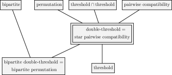
Figure 1: The hierarchy of graph classes mentioned in the introduction. The class of the edge-intersections of two threshold graphs is abbreviated as $\text{threshold}\cap\text{threshold}$. A line segment between two classes indicates that the one below is a subclass of the one above.

2 Preliminaries

All graphs in this paper are undirected, simple, and finite. A graph $G$ is given by the pair of its vertex set $V$ and its edge set $E$ as $G=(V,E)$. The vertex set and the edge set of $G$ are often denoted by $V(G)$ and $E(G)$, respectively. For a vertex $v$ in a graph $G=(V,E)$, its neighborhood is the set of vertices that are adjacent to $v$, and denoted by $N_{G}(v)=\{u\mid uv\in E\}$. When the graph $G$ is clear from the context, we often omit the subscript. A linear ordering $\prec$ on a set $S$ with $|S|=n$ can be represented by a sequence $\langle s_{1},s_{2},\dots,s_{n}\rangle$ of the elements in $S$, in which $s_{i}\prec s_{j}$ if and only if $i<j$. With abuse of notation, we sometimes write ${\prec}=\langle s_{1},s_{2},\dots,s_{n}\rangle$.

2.1 Double-threshold graphs

A graph $G=(V,E)$ is a threshold graph if there exist a vertex-weight function $\mathtt{w}\colon V\to\mathbb{R}$ and a real number $\mathtt{lb}\in\mathbb{R}$ with the following property:

$$uv\in E\iff\mathtt{lb}\leq\mathtt{w}(u)+\mathtt{w}(v).$$

A graph $G=(V,E)$ is a double-threshold graph if there exist a vertex-weight function $\mathtt{w}\colon V\to\mathbb{R}$ and two real numbers $\mathtt{lb},\mathtt{ub}\in\mathbb{R}$ with the following property:

$$uv\in E\iff\mathtt{lb}\leq\mathtt{w}(u)+\mathtt{w}(v)\leq\mathtt{ub}.$$

Then, we say that the double-threshold graph $G$ is defined by $\mathtt{w}$, $\mathtt{lb}$ and $\mathtt{ub}$.

Jamison and Sprague JamisonS20 showed that we can use any values as $\mathtt{lb}$ and $\mathtt{ub}$ for defining a double-threshold graph and that we do not have to consider degenerated cases, where some vertices have the same weight or some weight sum equals to the lower or upper bound.

Lemma 1 (JamisonS20 )

Let $G=(V,E)$ be a double-threshold graph. For every pair $\mathtt{lb},\mathtt{ub}\in\mathbb{R}$ with $\mathtt{lb}<\mathtt{ub}$, there exists $\mathtt{w}\colon V\to\mathbb{R}$ defining $G$ with $\mathtt{lb}$ and $\mathtt{ub}$ such that $\mathtt{w}(u)\neq\mathtt{w}(v)$ if $u\neq v$, and $\mathtt{w}(u)+\mathtt{w}(v)\notin\{\mathtt{lb},\mathtt{ub}\}$ for all $(u,v)\in V^{2}$.

Every threshold graph is a double-threshold graph as one can set a dummy upper bound $\mathtt{ub}>\max\{\mathtt{w}(u)+\mathtt{w}(v)\mid u,v\in V\}$. From the definition of double-threshold graphs, we can easily see that they coincide with the star pairwise compatibility graphs.

Observation 2.1

A graph is a double-threshold graph if and only if it is a star pairwise compatibility graph.

Proof

Let $G=(V,E)$ be a double-threshold graph defined by $\mathtt{w}\colon V\to\mathbb{R}$ and $\mathtt{lb},\mathtt{ub}\in\mathbb{R}$. We construct an edge-weighted star $S$ with the center $c$ and the leaf set $V$ such that the weight $\mathtt{w}^{\prime}(vc)$ of each edge $vc\in E(S)$ is $\mathtt{w}(v)$. Then, $G$ is the star pairwise compatibility graph defined by $(S,\mathtt{w}^{\prime},\mathtt{lb},\mathtt{ub})$.

Let $G=(V,E)$ be a star pairwise compatibility graph defined by $(S,\mathtt{w},\mathtt{lb},\mathtt{ub})$, where the star $S$ has $c$ as its center. For each $v\in V$, we set $\mathtt{w}^{\prime}(v)=\mathtt{w}(vc)$. Then, $G$ is the double-threshold graph defined by $\mathtt{w}^{\prime}$, $\mathtt{lb}$, and $\mathtt{ub}$.

Observation 2.1 allows us to state the following useful property shown by Xiao and Nagamochi XiaoN20 in terms of double-threshold graphs.

Lemma 2 (XiaoN20 )

A graph is a double-threshold graph if and only if it contains at most one non-bipartite component and all components are double-threshold graphs.

The following simple observation is useful when we conduct a detailed analysis on a specific triple $\mathtt{w}$, $\mathtt{lb}$, $\mathtt{ub}$ defining a double-threshold graph.

Observation 2.2

Let $G=(V,E)$ be a double-threshold graph defined by $\mathtt{w}\colon V\to\mathbb{R}$ and $\mathtt{lb},\mathtt{ub}\in\mathbb{R}$. If $\mathtt{w}(x)\leq\mathtt{w}(y)\leq\mathtt{w}(z)$ and $xy,yz\in E$ hold for distinct vertices $x,y,z\in V$, then $xz\in E$.

Proof

Since $\mathtt{lb}\leq\mathtt{w}(x)+\mathtt{w}(y)\leq\mathtt{w}(x)+\mathtt{w}(z)\leq\mathtt{w}(y)+\mathtt{w}(z)\leq\mathtt{ub}$, we have $xz\in E$.

The definition of double-threshold graphs can be understood visually in the plane, by its so called slab representation. See Figure 2 for an example. In the $xy$-plane, we consider the slab defined by $\{(x,y)\mid\mathtt{lb}\leq x+y\leq\mathtt{ub}\}$ that is illustrated in gray. Then, two vertices $u,v\in V$ are joined by an edge if and only if the point $(\mathtt{w}(u),\mathtt{w}(v))$ lies in the slab.

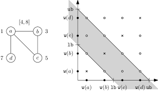
Figure 2: (Left) A double-threshold graph. The weight of each vertex is given as $\mathtt{w}(a)=1$, $\mathtt{w}(b)=3$, $\mathtt{w}(c)=5$, and $\mathtt{w}(d)=7$; the lower bound is $\mathtt{lb}=4$ and the upper bound is $\mathtt{ub}=8$. (Right) The slab representation of the graph. A white dot represents the point $(\mathtt{w}(u),\mathtt{w}(v))$ for distinct vertices $u,v$, and a cross represents the point $(\mathtt{w}(v),\mathtt{w}(v))$ for a vertex $v$. Two distinct vertices $u$ and $v$ are joined by an edge if and only if the corresponding white dot lies in the gray slab.

2.2 Permutation graphs

A graph $G=(V,E)$ is a permutation graph if there exist linear orderings $\prec_{1}$ and $\prec_{2}$ on $V$ with the following property:

$$uv\in E\iff(u\prec_{1}v\text{ and }v\prec_{2}u)\text{ or }(u\prec_{2}v\text{ and }v\prec_{1}u).$$ (1)

A graph is a bipartite permutation graph if it is a bipartite graph and a permutation graph. It is known that every permutation graph admits a transitive orientation Golumbic04 , which gives a direction to each edge in such a way that the existence of directed edges from $x$ to $y$ and from $y$ to $z$ implies a directed edge from $x$ to $z$ as well.

Jamison and Sprague JamisonS21 showed that permutation graphs and bipartite permutation graphs have strong connections to double-threshold graphs as follows.

Lemma 3 (JamisonS21 )

Every double-threshold graph is a permutation graph.

Lemma 4 (JamisonS21 )

The bipartite double-threshold graphs are exactly the bipartite permutation graphs.

We say that the orderings $\prec_{1}$ and $\prec_{2}$ in (1) define the permutation graph $G$. We call $\prec_{1}$ a permutation ordering of $G$ if there exists a linear ordering $\prec_{2}$ satisfying the condition above. Since $\prec_{1}$ and $\prec_{2}$ play a symmetric role in the definition, $\prec_{2}$ is also a permutation ordering of $G$. Note that for a graph $G$ and a permutation ordering $\prec_{1}$ of $G$, the other ordering $\prec_{2}$ that defines $G$ together with $\prec_{1}$ is uniquely determined. Also note that if $\prec_{1}$ and $\prec_{2}$ define $G$, then $\prec_{1}^{\mathrm{R}}$ and $\prec_{2}^{\mathrm{R}}$ also define $G$, where $\prec_{i}^{\mathrm{R}}$ denotes the reversed ordering of $\prec_{i}$.

We often represent a permutation graph with a permutation diagram, which is drawn as follows (see Figure 3 for an illustration). Imagine two horizontal parallel lines $\ell_{1}$ and $\ell_{2}$ on the plane. Then, we place the vertices in $V$ on $\ell_{1}$ from left to right according to the permutation ordering $\prec_{1}$ as distinct points, and similarly place the vertices in $V$ on $\ell_{2}$ from left to right according to $\prec_{2}$ as distinct points. The positions of $v\in V$ can be represented by $x$-coordinates on $\ell_{1}$ and $\ell_{2}$, which are denoted by $\mathtt{x}_{1}(v)$ and $\mathtt{x}_{2}(v)$, respectively. We connect the two points representing the same vertex with a line segment. The process results in a diagram (called a permutation diagram) with $|V|$ line segments. By definition, $uv\in E$ if and only if the line segments representing $u$ and $v$ cross in the permutation diagram, which is equivalent to the inequality $(\mathtt{x}_{1}(u)-\mathtt{x}_{1}(v))(\mathtt{x}_{2}(u)-\mathtt{x}_{2}(v))<0$.

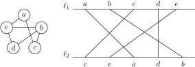
Figure 3: An example of a permutation diagram. (Left) A permutation graph $G$. (Right) A permutation diagram that represents $G$.

Conversely, from a permutation diagram of $G$, we can extract linear orderings $\prec_{1}$ and $\prec_{2}$ as

$$\mathtt{x}_{1}(u)<\mathtt{x}_{1}(v) \iff u\prec_{1}v,$$

$$\mathtt{x}_{2}(u)<\mathtt{x}_{2}(v) \iff u\prec_{2}v.$$

When those conditions are satisfied, we say that the orderings of the $x$-coordinates on $\ell_{1}$ and $\ell_{2}$ are consistent with the linear orderings $\prec_{1}$ and $\prec_{2}$, respectively.

Although a permutation graph may have an exponential number of permutation orderings, it is essentially unique for a connected bipartite permutation graph in the sense of Lemma 5 below. For a graph $G=(V,E)$, linear orderings $\langle v_{1},\dots,v_{n}\rangle$ and $\langle v^{\prime}_{1},\dots,v^{\prime}_{n}\rangle$ on $V$ are neighborhood-equivalent if $N(v_{i})=N(v^{\prime}_{i})$ for all $i$.

Lemma 5 (HeggernesHMV15 )

Let $G$ be a connected bipartite permutation graph defined by $\prec_{1}$ and $\prec_{2}$. Then, every permutation ordering of $G$ is neighborhood-equivalent to $\prec_{1}$, $\prec_{2}$, $\prec_{1}^{\mathrm{R}}$, or $\prec_{2}^{\mathrm{R}}$.

A bipartite graph $(X,Y;E)$ is a unit interval bigraph if there is a set of unit intervals $\{I_{v}=[l_{v},l_{v}+1]\mid v\in X\cup Y\}$ such that $xy\in E$ if and only if $I_{x}\cap I_{y}\neq\emptyset$ for $x\in X$ and $y\in Y$. The class of unit interval bigraphs is known to be equal to the class of bipartite permutation graphs.

Proposition 1 (HellH04 ; SenS94 ; West98 )

A graph is a bipartite permutation graph if and only if it is a unit interval bigraph.

The following lemma shows that a bipartite permutation graph can be represented by a permutation diagram with the special property that the segments representing vertices of the same set of the bipartition are parallel. An illustration is given in Figure 4.

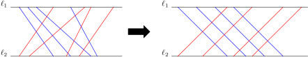
Figure 4: An illustration of Lemma 6. (Left) A permutation diagram of a bipartite permutation graph $G=(X,Y;E)$. The vertices in $X$ are represented by blue segments, and the vertices in $Y$ are represented by red segments. (Right) A permutation diagram that represents $G$ obtained by Lemma 6.

Lemma 6

Let $G=(X,Y;E)$ be a bipartite permutation graph. Then, $G$ can be represented by a permutation diagram in which $\mathtt{x}_{2}(x)=\mathtt{x}_{1}(x)+1$ for $x\in X$ and $\mathtt{x}_{2}(y)=\mathtt{x}_{1}(y)-1$ for $y\in Y$.

Proof

By Proposition 1, there is a set of unit intervals $\{I_{v}=[l_{v},l_{v}+1]\mid v\in X\cup Y\}$ such that for $x\in X$ and $y\in Y$, $xy\in E$ if and only if $I_{x}\cap I_{y}\neq\emptyset$. We can assume that all endpoints of the intervals are distinct; that is, $l_{u}\notin\{l_{v},l_{v}+1\}$ for all $u,v\in X\cup Y$ with $u\neq v$ West98 . For each $x\in X$, we set $\mathtt{x}_{1}(x)=l_{x}$ and $\mathtt{x}_{2}(x)=l_{x}+1$. For each $y\in Y$, we set $\mathtt{x}_{1}(y)=l_{y}+1$ and $\mathtt{x}_{2}(y)=l_{y}$. It suffices to show that this permutation diagram represents $G$. Observe that line segments corresponding to vertices from the same set, $X$ or $Y$, are parallel and thus do not cross. For $x\in X$ and $y\in Y$, we have

$$I_{x}\cap I_{y}\neq\emptyset \iff|l_{x}-l_{y}|<1 (\because\text{ all endpoints are distinct})$$

$$\iff l_{x}<l_{y}+1\textrm{ and }l_{y}<l_{x}+1$$

$$\iff\mathtt{x}_{1}(x)<\mathtt{x}_{1}(y)\textrm{ and }\mathtt{x}_{2}(y)<\mathtt{x}_{2}(x) (\because x\in X,\ y\in Y)$$

$$\iff(\mathtt{x}_{1}(x)-\mathtt{x}_{1}(y))(\mathtt{x}_{2}(x)-\mathtt{x}_{2}(y))<0.$$

The $\Leftarrow$ direction of the last equivalence holds since $\mathtt{x}_{1}(x)<\mathtt{x}_{2}(x)$ and $\mathtt{x}_{1}(y)>\mathtt{x}_{2}(y)$. Therefore, we conclude that the diagram represents $G$.

We can show that for every permutation ordering of a connected bipartite permutation graph, there exists a permutation diagram consistent with the ordering that satisfies the conditions in Lemma 6.

Corollary 1

Let $G=(X,Y;E)$ be a connected bipartite permutation graph defined by permutation orderings $\prec_{1}$ and $\prec_{2}$. If the first vertex in $\prec_{1}$ belongs to $X$, then $G$ can be represented by a permutation diagram such that the orderings of the $x$-coordinates on $\ell_{1}$ and $\ell_{2}$ are consistent with $\prec_{1}$ and $\prec_{2}$, respectively, and that $\mathtt{x}_{2}(x)=\mathtt{x}_{1}(x)+1$ for every $x\in X$ and $\mathtt{x}_{2}(y)=\mathtt{x}_{1}(y)-1$ for every $y\in Y$.

Proof

Since $G$ is connected, the last vertex in $\prec_{1}$ belongs to $Y$, the first vertex in $\prec_{2}$ belongs to $Y$, and the last vertex in $\prec_{2}$ belongs to $X$.

By Lemma 6, $G$ can be represented by a permutation diagram $D^{\prime}$ in which $\mathtt{x}_{2}(x)=\mathtt{x}_{1}(x)+1$ for $x\in X$ and $\mathtt{x}_{2}(y)=\mathtt{x}_{1}(y)-1$ for $y\in Y$. Let $\prec^{\prime}_{1}$ and $\prec^{\prime}_{2}$ be the permutation orderings corresponding to $\ell_{1}$ and $\ell_{2}$, respectively, in this diagram $D^{\prime}$. Lemma 5 and the assumption on the first vertex in $\prec_{1}$ imply that $\prec_{1}$ is neighborhood-equivalent to $\prec^{\prime}_{1}$ or $(\prec^{\prime}_{2})^{R}$. We may assume that $\prec_{1}$ is neighborhood-equivalent to $\prec^{\prime}_{1}$ since otherwise we can rotate the diagram $D^{\prime}$ by $180$ degrees and get a permutation diagram of $G$ in which the ordering on $\ell_{1}$ is $\prec_{1}$, $\mathtt{x}_{2}(x)=\mathtt{x}_{1}(x)+1$ for $x\in X$, and $\mathtt{x}_{2}(y)=\mathtt{x}_{1}(y)-1$ for $y\in Y$.

Now we can construct a desired permutation diagram of $G$ using $\prec_{1}$ and $D^{\prime}$ by appropriately giving a mapping between segments and vertices. That is, for each $i\in\{1,\dots,|X\cup Y|\}$, we assign the $i$th vertex in $\prec_{1}$ to the segment in $D^{\prime}$ with the $i$th smallest $x$-coordinate on $\ell_{1}$. This new diagram is a permutation diagram of $G$ since $\prec_{1}$ is neighborhood-equivalent to $\prec^{\prime}_{1}$. Since $G$ and $\prec_{1}$ uniquely determine the ordering on $\ell_{2}$, the $x$-coordinates $\mathtt{x}_{2}$ on $\ell_{2}$ are consistent with $\prec_{2}$.

3 New characterization

In this section, we present a new characterization of double-threshold graphs (Theorem 3.1). This is one of our main results and a key ingredient of the linear-time algorithm given in the next section. Recall that Lemma 4 characterizes the bipartite double-threshold graphs as the bipartite permutation graphs, which can be recognized in linear time SpinradBS87 ; Sprague95 . Thus, we are going to focus on non-bipartite graphs in this section.

Let $G=(V,E)$ be a graph. From $G$ and a vertex subset $M\subseteq V$, we construct an auxiliary bipartite graph $G^{\prime}_{M}=(V^{\prime},E^{\prime})$ defined as follows (see Figure 5):

$$V^{\prime} =\{v,\overline{v}\mid v\in V\}, E^{\prime} =\{u\overline{v}\mid uv\in E\}\cup\{v\overline{v}\mid v\in M\}.$$

Note that $(V,\{\overline{v}\mid v\in V\})$ is a bipartition of $G^{\prime}_{M}$ no matter what $M$ is.

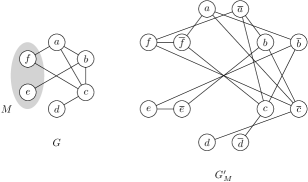
Figure 5: An example of an auxiliary bipartite graph. (Left) A graph $G$ and $M=\{e,f\}$. (Right) The auxiliary bipartite graph $G^{\prime}_{M}$.

An efficient maximum clique $K$ of a graph $G$ is a maximum clique (i.e., a clique of the maximum size) that minimizes the degree sum $\sum_{v\in K}\deg_{G}(v)$. See Figure 6.

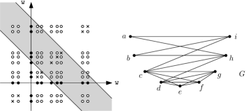
Figure 6: An example of an efficient maximum clique. (Left) A slab representation of a double-threshold graph $G$. (Right) The vertices of $G$ are ordered in the increasing order of their weights. The graph $G$ has two maximum cliques $Q_{1}=\{c,e,f,g\}$ and $Q_{2}=\{d,e,f,g\}$. The degree sums are $\sum_{v\in Q_{1}}\deg_{G}(v)=5+4+4+4=17$, and $\sum_{v\in Q_{2}}\deg_{G}(v)=4+4+4+4=16$. Therefore, $Q_{2}$ is the only efficient maximum clique of $G$.

Using these terms, we present a characterization of non-bipartite double-threshold graphs as follows.

Theorem 3.1 ()

For a non-bipartite graph $G$, the following are equivalent.

1. $G$ is a double-threshold graph.

2. For every efficient maximum clique $M$ of $G$, the graph $G^{\prime}_{M}$ is a bipartite permutation graph.

3. For some efficient maximum clique $M$ of $G$, the graph $G^{\prime}_{M}$ is a bipartite permutation graph.

The rest of this section is devoted to a proof of Theorem 3.1. The following is a quick overview of the proof steps (some terms will be defined later).

1. We first prove the key lemma (Lemma 8) ensuring that a graph is a double-threshold graph if and only if $G^{\prime}_{M}$ is a permutation graph with a “symmetric” permutation diagram, where $M\subseteq V$ is the set of “mid-weight” vertices.

2. We then show that every efficient maximum clique can be the set of mid-weight vertices by proving a couple of lemmas (Lemmas 9 and 10).

3. Next, we show that the symmetry required in the key lemma follows for free if $M$ is a clique (Lemma 11), which is true when we set $M$ to be the set of mid-weight vertices.

4. Finally, we complete the proof of Theorem 3.1 by putting everything together.

We start with the following simple but useful fact.

Lemma 7

For a connected non-bipartite graph $G=(V,E)$ and a vertex subset $M\subseteq V$, $G^{\prime}_{M}$ is connected.

Proof

For any $u,v\in V$, since $G$ is connected and non-bipartite, $G$ contains both an odd walk and an even walk from $u$ to $v$. This shows that $G^{\prime}_{M}$ contains walks from $u$ to $v$, from $u$ to $\bar{v}$, from $\bar{u}$ to $v$, and from $\bar{u}$ to $\bar{v}$. Hence, $G^{\prime}_{M}$ is connected.

For the auxiliary graph $G^{\prime}_{M}=(V^{\prime},E^{\prime})$ of $G=(V,E)$, a linear ordering on $V^{\prime}$ represented by $\langle w_{1},w_{2},\dots,w_{2n}\rangle$ is symmetric if $w_{i}=v$ implies $w_{2n-i+1}=\bar{v}$ for any $v\in V$ and any $i\in\{1,2,\dots,2n\}$.

Lemma 8

Let $G=(V,E)$ be a non-bipartite graph and $M\subseteq V$. The following are equivalent.

1. $G$ is a double-threshold graph defined by $\mathtt{w}\colon V\to\mathbb{R}$ and $\mathtt{lb},\mathtt{ub}\in\mathbb{R}$ such that $M=\{v\in V\mid\mathtt{lb}/2\leq\mathtt{w}(v)\leq\mathtt{ub}/2\}$.

2. The auxiliary graph $G^{\prime}_{M}=(V^{\prime},E^{\prime})$ can be represented by a permutation diagram in which both orderings $\prec_{1}$ and $\prec_{2}$ are symmetric.

Proof

(1$\implies$2) An illustration is given in Figure 7. Let $G$ be a double-threshold graph defined by $\mathtt{w}\colon V\to\mathbb{R}$ and $\mathtt{lb},\mathtt{ub}\in\mathbb{R}$ such that $M=\{v\in V\mid\mathtt{lb}/2\leq\mathtt{w}(v)\leq\mathtt{ub}/2\}$. By Lemma 1, we can assume that $\mathtt{lb}=0$ and $\mathtt{ub}=2$, that $\mathtt{w}(u)+\mathtt{w}(v)\notin\{0,2\}$ for every $(u,v)\in V^{2}$, and that $\mathtt{w}(u)\neq\mathtt{w}(v)$ if $u\neq v$. We construct a permutation diagram of $G^{\prime}_{M}$ as follows. Let $\ell_{1}$ and $\ell_{2}$ be two horizontal parallel lines. For each vertex $w\in V^{\prime}$, we set the $x$-coordinates $\mathtt{x}_{1}(w)$ and $\mathtt{x}_{2}(w)$ on $\ell_{1}$ and $\ell_{2}$ as follows: for any $v\in V$,

$$\mathtt{x}_{1}(v) =\mathtt{w}(v)-1, \mathtt{x}_{1}(\bar{v}) =1-\mathtt{w}(v),$$

$$\mathtt{x}_{2}(v) =\mathtt{w}(v), \mathtt{x}_{2}(\bar{v}) =-\mathtt{w}(v).$$

Since $\mathtt{w}(u)+\mathtt{w}(v)\notin\{0,2\}$ for every $(u,v)\in V^{2}$ and $\mathtt{w}(u)\neq\mathtt{w}(v)$ if $u\neq v$, the $x$-coordinates are distinct on $\ell_{1}$ and on $\ell_{2}$. By connecting $\mathtt{x}_{1}(w)$ and $\mathtt{x}_{2}(w)$ with a line segment for each $w\in V^{\prime}$, we get a permutation diagram. The line segments corresponding to the vertices in $V$ have negative slopes, and the ones corresponding to the vertices in $V^{\prime}\setminus V$ have positive slopes. Thus, for any two vertices $u,v\in V$, the line segments corresponding to $u$ and $\bar{v}$ cross if and only if both $\mathtt{x}_{1}(u)\leq\mathtt{x}_{1}(\bar{v})$ and $\mathtt{x}_{2}(u)\geq\mathtt{x}_{2}(\bar{v})$ hold, which is equivalent to $0\leq\mathtt{w}(u)+\mathtt{w}(v)\leq 2$, and thus to $u\bar{v}\in E^{\prime}$. Similarly, the line segments corresponding to $v$ and $\bar{v}$ cross if and only if $0\leq 2\mathtt{w}(v)\leq 2$, i.e., $v\in M$. This shows that the obtained permutation diagram represents $G^{\prime}_{M}$. Let $\prec_{1}$ be the ordering on $V^{\prime}$ defined by $\mathtt{x}_{1}$. Since $\mathtt{x}_{1}(v)=-\mathtt{x}_{1}(\bar{v})$ for each $v\in V$, $\prec_{1}$ is symmetric. Similarly, the ordering $\prec_{2}$ defined by $\mathtt{x}_{2}$ is symmetric.

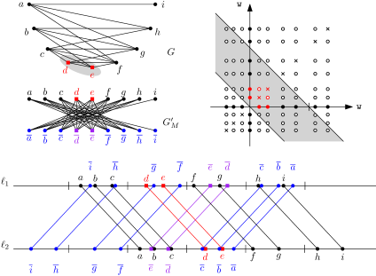
Figure 7: An illustration of (1 $\implies$ 2) in Lemma 8. (Top left) A double-threshold graph $G$ with $M=\{d,e\}$. The auxiliary bipartite graph $G^{\prime}_{M}$ is also depicted. (Top right) A slab representation of $G$. (Bottom) A permutation diagram of $G^{\prime}_{M}$ as given in the proof.

(2$\implies$1) Suppose we are given a permutation diagram of $G^{\prime}_{M}$ in which both $\prec_{1}$ and $\prec_{2}$ are symmetric. We may assume by symmetry that the first vertex in $\prec_{1}$ belongs to $V$. Since $G^{\prime}_{M}$ is connected by Lemma 7, Corollary 1 shows that we can represent $G^{\prime}_{M}$ by a permutation diagram in which the $x$-coordinates $\mathtt{x}_{1}$ and $\mathtt{x}_{2}$ on $\ell_{1}$ and $\ell_{2}$ satisfy that

$$\mathtt{x}_{2}(v)=\mathtt{x}_{1}(v)+1\quad\mbox{and}\quad\mathtt{x}_{2}(\bar{v})=\mathtt{x}_{1}(\bar{v})-1\quad(v\in V)$$ (2)

and that the orderings of the $x$-coordinates on $\ell_{1}$ and $\ell_{2}$ are consistent with $\prec_{1}$ and $\prec_{2}$, respectively. Since $\prec_{1}$ is symmetric, if $u,v\in V$ are the $i$th and the $j$th vertices in $\prec_{1}$, then $\bar{u},\bar{v}$ are the $(2n-i+1)$st and the $(2n-j+1)$st vertices in $\prec_{1}$. Since $i<2n-j+1$ is equivalent to $j<2n-i+1$, we have that $u\prec_{1}\bar{v}$ if and only if $v\prec_{1}\bar{u}$. As $\mathtt{x}_{1}$ is consistent with $\prec_{1}$, it holds for $u,v\in V$ that $\mathtt{x}_{1}(u)\leq\mathtt{x}_{1}(\bar{v})$ if and only if $\mathtt{x}_{1}(v)\leq\mathtt{x}_{1}(\bar{u})$, and hence

$$\mathtt{x}_{1}(u)\leq\mathtt{x}_{1}(\bar{v})\iff\mathtt{x}_{1}(u)+\mathtt{x}_{1}(v)\leq\mathtt{x}_{1}(\bar{v})+\mathtt{x}_{1}(\bar{u}).$$

Similarly, we can show that for $u,v\in V$,

$$\mathtt{x}_{2}(u)\geq\mathtt{x}_{2}(\bar{v})\iff\mathtt{x}_{2}(u)+\mathtt{x}_{2}(v)\geq\mathtt{x}_{2}(\bar{v})+\mathtt{x}_{2}(\bar{u}).$$

Thus, for any two distinct vertices $u,v\in V$, it holds that

$$uv\in E \iff u\bar{v}\in E^{\prime}$$

$$\iff\mathtt{x}_{1}(u)\leq\mathtt{x}_{1}(\bar{v})\mbox{ and }\mathtt{x}_{2}(u)\geq\mathtt{x}_{2}(\bar{v})$$

$$\iff\mathtt{x}_{1}(u)+\mathtt{x}_{1}(v)\leq\mathtt{x}_{1}(\bar{v})+\mathtt{x}_{1}(\bar{u})\mbox{ and }\mathtt{x}_{2}(u)+\mathtt{x}_{2}(v)\geq\mathtt{x}_{2}(\bar{v})+\mathtt{x}_{2}(\bar{u}).$$ (3)

For each $v\in V$, define

$$\mathtt{w}(v)=\frac{\mathtt{x}_{2}(v)-\mathtt{x}_{2}(\bar{v})}{2}.$$

By (2), we can see that (3) is equivalent to

$$0\leq\mathtt{w}(u)+\mathtt{w}(v)\leq 2,$$

which shows that $\mathtt{w}$, $\mathtt{lb}=0$, and $\mathtt{ub}=2$ define $G$. Furthermore, for any $v\in V$,

$$v\in M \iff v\bar{v}\in E^{\prime}$$

$$\iff\mathtt{x}_{1}(v)\leq\mathtt{x}_{1}(\bar{v})\mbox{ and }\mathtt{x}_{2}(v)\geq\mathtt{x}_{2}(\bar{v})$$

$$\iff 0\leq\mathtt{w}(v)\leq 1,$$

which shows that $M=\{v\in V\mid 0\leq\mathtt{w}(v)\leq 1\}$.

To utilize Lemma 8, we need to find the set $M$ of mid-weight vertices; that is, the vertices with weights in the range $[\mathtt{lb}/2,\mathtt{ub}/2]$. The first observation is that $M$ has to be a clique as the weight sum of any two vertices in $M$ is in the range $[\mathtt{lb},\mathtt{ub}]$. In the following, we show that an efficient maximum clique can be chosen as $M$. To this end, we first prove that we only need to consider (inclusion-wise) maximal cliques.

Lemma 9

For a connected non-bipartite double-threshold graph $G=(V,E)$, there exist $\mathtt{w}\colon V\to\mathbb{R}$ and $\mathtt{lb},\mathtt{ub}\in\mathbb{R}$ defining $G$ such that $\{v\in V\mid\mathtt{lb}/2\leq\mathtt{w}(v)\leq\mathtt{ub}/2\}$ is a maximal clique of $G$.

Proof

Let $G$ be a non-bipartite double-threshold graph $G=(V,E)$ defined by $\mathtt{w}\colon V\to\mathbb{R}$ and $\mathtt{lb},\mathtt{ub}\in\mathbb{R}$. Let $M=\{v\in V\mid\mathtt{lb}/2\leq\mathtt{w}(v)\leq\mathtt{ub}/2\}$. We choose $\mathtt{w}$, $\mathtt{lb}$, and $\mathtt{ub}$ in such a way that for any $\mathtt{w}^{\prime}\colon V\to\mathbb{R}$ and $\mathtt{lb}^{\prime},\mathtt{ub}^{\prime}\in\mathbb{R}$ defining $G$, $M$ is not a proper subset of $\{v\in V\mid\mathtt{lb}^{\prime}/2\leq\mathtt{w}^{\prime}(v)\leq\mathtt{ub}^{\prime}/2\}$. Suppose to the contrary that $M$ is not a maximal clique of $G$. Observe that if $M=\emptyset$, then $V$ can be partitioned into two independent sets $\{v\in V\mid\mathtt{w}(v)<\mathtt{lb}/2\}$ and $\{v\in V\mid\mathtt{w}(v)>\mathtt{ub}/2\}$, which is a contradiction to the non-bipartiteness of $G$. Hence, $M$ is non-empty.

Let $G^{\prime}_{M}$ be the auxiliary graph constructed from $G$ and $M$ as before. By Lemma 8, $G^{\prime}_{M}$ has a permutation diagram in which both ${\prec_{1}}=\langle w_{1},\dots,w_{2n}\rangle$ and ${\prec_{2}}=\langle w^{\prime}_{1},\dots,w^{\prime}_{2n}\rangle$ are symmetric. Let $\overline{M}=\{\bar{v}\mid v\in M\}$. By the definition of $G^{\prime}_{M}$, $M\cup\overline{M}$ induces a complete bipartite graph in $G^{\prime}_{M}$. By symmetry, we may assume that $M\prec_{1}\overline{M}$ and $\overline{M}\prec_{2}M$. That is, in $\prec_{1}$ all vertices in $M$ appear before any vertex in $\overline{M}$ appears, and in $\prec_{2}$ all vertices in $\overline{M}$ appear before any vertex in $M$ appears. Note that these assumptions imply that for each edge $x\bar{y}\in E(G^{\prime}_{M})$, $x\prec_{1}\bar{y}$ and $\bar{y}\prec_{2}x$ hold since $G^{\prime}_{M}$ is connected by Lemma 7 (see Figure 8 (Left)).

As $M$ is not a maximal clique in $G$, there is a vertex $v\notin M$ such that $M\subseteq N_{G}(v)$. If $\bar{v}\prec_{1}v$, then we have

$$M\prec_{1}\bar{v}\prec_{1}v\prec_{1}\overline{M}\quad\text{ and }\quad\bar{v}\prec_{2}\overline{M}\prec_{2}M\prec_{2}v$$ (4)

since $v\bar{v}\notin E(G^{\prime}_{M})$, $\overline{M}\subseteq N_{G^{\prime}_{M}}(v)$, and $M\subseteq N_{G^{\prime}_{M}}(\bar{v})$. Similarly, if $v\prec_{1}\bar{v}$, then we have

$$v\prec_{1}M\prec_{1}\overline{M}\prec_{1}\bar{v}\quad\text{ and }\quad\overline{M}\prec_{2}v\prec_{2}\bar{v}\prec_{2}M,$$

or equivalently,

$$M\prec_{2}^{R}\bar{v}\prec_{2}^{R}v\prec_{2}^{R}\overline{M}\quad\text{ and }\quad\bar{v}\prec_{1}^{R}\overline{M}\prec_{1}^{R}M\prec_{1}^{R}v.$$

Thus, by replacing $\prec_{1}$ with $\prec_{2}^{R}$ and $\prec_{2}$ with $\prec_{1}^{R}$ if necessary, we may assume that (4) holds (see Figure 8 (Left)). We further assume that $v$ has the smallest position in $\prec_{1}$ under these conditions.

Claim 3.2

$w_{n+1}=v$ (and thus $w_{n}=\bar{v}$).

Proof (Claim 3.2)

By the symmetry of $\langle w_{1},\dots,w_{2n}\rangle$, it suffices to show that there is no vertex $x\in V$ such that $\bar{v}\prec_{1}x\prec_{1}v$. Suppose that such a vertex $x$ exists. In $G^{\prime}_{M}$, $x$ is not adjacent to $\bar{v}$. This implies that $xv\notin E$, and hence $x\notin M$. On the other hand, in $G^{\prime}_{M}$, $x$ is adjacent to all vertices in $\overline{M}$. Thus, we have $M\subseteq N_{G}(x)$. This contradicts that $v$ has the smallest position in $\prec_{1}$ under those conditions.

Now we obtain $\prec^{\prime}_{1}$ from $\prec_{1}$ by swapping $v$ and $\bar{v}$ (see Figure 8 (Right)). By Claim 3.2, this new ordering $\prec^{\prime}_{1}$ gives (together with $\prec_{2}$) the graph obtained from $G^{\prime}_{M}$ by adding the edge $v\bar{v}$. Observe that this new graph can be expressed as $G^{\prime}_{M\cup\{v\}}$. Since $\prec^{\prime}_{1}$ and $\prec_{2}$ are symmetric, Lemma 8 implies that there are $\mathtt{w}^{\prime}\colon V\to\mathbb{R}$ and $\mathtt{lb}^{\prime},\mathtt{ub}^{\prime}\in\mathbb{R}$ defining $G$ such that $\{u\in V\mid\mathtt{lb}^{\prime}/2\leq\mathtt{w}^{\prime}(u)\leq\mathtt{ub}^{\prime}/2\}=M\cup\{v\}$. This contradicts the choice of $\mathtt{w}$, $\mathtt{lb}$, and $\mathtt{ub}$.

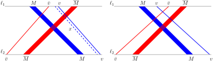
Figure 8: (Left) Relative positions of $v$, $\bar{v}$, $M$, and $\overline{M}$. (Right) $\prec^{\prime}_{1}$ is obtained from $\prec_{1}$ by swapping $v$ and $\bar{v}$.

We show that every efficient maximum clique can be the set of mid-weight vertices, given an appropriate choice of $\mathtt{w}$, $\mathtt{lb}$, and $\mathtt{ub}$.

Lemma 10

Let $G$ be a non-bipartite double-threshold graph. For every efficient maximum clique $K$ of $G$, there exist $\mathtt{w}\colon V\to\mathbb{R}$ and $\mathtt{lb},\mathtt{ub}\in\mathbb{R}$ defining $G$ such that $K=\{v\in V\mid\mathtt{lb}/2\leq\mathtt{w}(v)\leq\mathtt{ub}/2\}$.

Proof

Let $K$ be an efficient maximum clique of $G$. By Lemma 3, $G$ is a permutation graph, and thus cannot contain an induced odd cycle of length $5$ or more Golumbic04 . As $G$ is non-bipartite, $G$ contains $K_{3}$. This implies that $|K|\geq 3$.

By Lemma 9, there exist $\mathtt{w}\colon V\to\mathbb{R}$ and $\mathtt{lb},\mathtt{ub}\in\mathbb{R}$ defining $G$ such that $M:=\{v\in V\mid\mathtt{lb}/2\leq\mathtt{w}(v)\leq\mathtt{ub}/2\}$ is a maximal clique of $G$. Assume that $\mathtt{w}$, $\mathtt{lb}$, and $\mathtt{ub}$ are chosen so that the size of the symmetric difference $|M\vartriangle K|=|M\setminus K|+|K\setminus M|$ is minimized. Assume that $K\neq M$ since otherwise we are done. This implies that $K\not\subseteq M$ and $K\not\supseteq M$ as both $K$ and $M$ are maximal cliques. Observe that $G-M$ is bipartite. This implies that $|K\setminus M|\in\{1,2\}$ and that $K\cap M\neq\emptyset$ as $|K|\geq 3$. Since $K$ is a maximum clique, $|M\setminus K|\leq|K\setminus M|$ holds.

Let $u\in K\setminus M$. By symmetry, we may assume that $\mathtt{w}(u)<\mathtt{lb}/2$. Note that no other vertex in $K$ has weight less than $\mathtt{lb}/2$ as $K$ is a clique. Let $v\in M$ be a non-neighbor of $u$ that has the minimum weight among such vertices. Such a vertex exists since $M$ is a maximal clique. Note that $v\in M\setminus K$.

We now observe that $v$ has the minimum weight in $M$. If $w\in M$ is a non-neighbor of $u$, then $\mathtt{w}(v)\leq\mathtt{w}(w)$ follows from the definition of $v$. If $w\in M$ is a neighbor of $u$, then $\mathtt{w}(v)<\mathtt{w}(w)$ holds, since otherwise $\mathtt{w}(u)<\mathtt{lb}/2\leq\mathtt{w}(w)\leq\mathtt{w}(v)$ and $uw,wv\in E$ imply that $uv\in E$ by Observation 2.2.

We are going to show that $N(v)=N(u)$.

Claim 3.3

$N(u)\cap\{x\mid\mathtt{w}(x)<\mathtt{lb}/2\}=N(v)\cap\{x\mid\mathtt{w}(x)<\mathtt{lb}/2\}=\emptyset$.

Proof (Claim 3.3)

Since $\mathtt{w}(u)<\mathtt{lb}/2$, $N(u)\cap\{x\mid\mathtt{w}(x)<\mathtt{lb}/2\}=\emptyset$. Suppose to the contrary that $v$ has a neighbor $x$ with $\mathtt{w}(x)<\mathtt{lb}/2$. The maximality of $M$ implies that $x$ has a non-neighbor $y\in M$. Since $y\in M$, $\mathtt{w}(v)\leq\mathtt{w}(y)$ holds. However, $\mathtt{w}(x)<\mathtt{lb}/2\leq\mathtt{w}(v)\leq\mathtt{w}(y)$ and $xv,vy\in E$ imply $xy\in E$ by Observation 2.2.

Claim 3.4

$N(u)\cap M=N(v)\cap M=M\setminus\{v\}$.

Proof (Claim 3.4)

Since $M$ is a clique and $v\in M$, we have $N(v)\cap M=M\setminus\{v\}$. Thus, the claim is equivalent to $M\setminus\{v\}\subseteq N(u)$. This holds if $M\setminus K=\{v\}$. Assume that $M\setminus K=\{v,v^{\prime}\}$ for some $v^{\prime}\neq v$. To show the claim, it suffices to show that $uv^{\prime}\in E$.

Since $|M\setminus K|\leq|K\setminus M|\leq 2$, we have $K\setminus M=\{u,u^{\prime}\}$ for some $u^{\prime}\neq u$. Since $\mathtt{w}(u)<\mathtt{lb}/2$ and $uu^{\prime}\in E$, we have $\mathtt{w}(u^{\prime})\geq\mathtt{lb}/2$. Moreover since $u^{\prime}\notin M$, we have $\mathtt{w}(u^{\prime})>\mathtt{ub}/2$. Let $w\in M\cap K$. If $\mathtt{w}(w)>\mathtt{w}(v^{\prime})$, then, by Observation 2.2, we have $u^{\prime}v,u^{\prime}v^{\prime}\in E$ since $\mathtt{w}(v)\leq\mathtt{w}(v^{\prime})<\mathtt{w}(w)\leq\mathtt{w}(u^{\prime})$ and $vw,v^{\prime}w,wu^{\prime}\in E$. This implies that $M\subseteq N(u^{\prime})$, which contradicts the maximality of $M$. Hence, $\mathtt{w}(w)\leq\mathtt{w}(v^{\prime})$ holds. This implies by Observation 2.2 that $uv^{\prime}\in E$ as $\mathtt{w}(u)\leq\mathtt{w}(w)\leq\mathtt{w}(v^{\prime})$ and $uw,wv^{\prime}\in E$.

Claim 3.5

$N(u)\cap\{x\mid\mathtt{w}(x)>\mathtt{ub}/2\}\supseteq N(v)\cap\{x\mid\mathtt{w}(x)>\mathtt{ub}/2\}$.

Proof (Claim 3.5)

Let $w\in K\cap M$. For $z\in N(v)$ with $\mathtt{w}(z)>\mathtt{ub}/2$, we have

$$\mathtt{lb}\leq\mathtt{w}(u)+\mathtt{w}(w)\leq\mathtt{w}(u)+\mathtt{ub}/2<\mathtt{w}(u)+\mathtt{w}(z)<\mathtt{lb}/2+\mathtt{w}(z)<\mathtt{w}(v)+\mathtt{w}(z)\leq\mathtt{ub},$$

and thus $z\in N(u)$ holds.

Claims 3.3, 3.4, and 3.5 imply that $N(v)\subseteq N(u)$. To show that $N(v)=N(u)$, suppose to the contrary that $N(v)$ is a proper subset of $N(u)$. We show that $K$ cannot be an efficient maximum clique in this case. Let $K^{\prime}=K\setminus\{u\}\cup\{v\}$. We first argue that $K^{\prime}$ is a maximum clique. To this end, it suffices to show that $K^{\prime}$ is a clique as $|K^{\prime}|=|K|$. If $K\setminus M=\{u\}$, then $K^{\prime}=M$ is a clique. Assume that $K\setminus M=\{u,u^{\prime}\}$ for some $u^{\prime}\neq u$. Since $\mathtt{w}(u)<\mathtt{lb}/2$ and $u^{\prime}\in K\setminus M$, we have $\mathtt{w}(u^{\prime})>\mathtt{ub}/2$ as before. Let $w\in K\cap M$. Then, $vw,wu^{\prime}\in E$. Since $\mathtt{w}(v)\leq\mathtt{w}(w)\leq\mathtt{ub}/2<\mathtt{w}(u^{\prime})$, we have $vu^{\prime}\in E$ by Observation 2.2. Thus, $K^{\prime}$ is a clique. The assumption $N(v)\subsetneq N(u)$ implies that $\deg_{G}(v)<\deg_{G}(u)$, and thus,

$$\sum_{w\in K^{\prime}}\deg_{G}(w)=\left(\sum_{w\in K}\deg_{G}(w)\right)-\deg_{G}(u)+\deg_{G}(v)<\sum_{w\in K}\deg_{G}(w).$$

This contradicts that $K$ is efficient. Therefore, we conclude that $N(v)=N(u)$.

Now, we define a weight function $\mathtt{w}^{\prime}\colon V\to\mathbb{R}$ by setting $\mathtt{w}^{\prime}(u)=\mathtt{w}(v)$, $\mathtt{w}^{\prime}(v)=\mathtt{w}(u)$, and $\mathtt{w}^{\prime}(x)=\mathtt{w}(x)$ for all $x\in V\setminus\{u,v\}$. Then, $\mathtt{w}^{\prime}$, $\mathtt{lb}$, and $\mathtt{ub}$ define $G$ and $M^{\prime}:=\{w\in V\mid\mathtt{lb}/2\leq\mathtt{w}^{\prime}(w)\leq\mathtt{ub}/2\}=M\cup\{u\}\setminus\{v\}$ as $N(u)=N(v)$. This contradicts the choice of $\mathtt{w}$ as $|M^{\prime}\vartriangle K|<|M\vartriangle K|$.

Next, we show that the symmetry required in Lemma 8 follows for free when $M$ is a clique.

Lemma 11

Let $G=(V,E)$ be a connected non-bipartite graph and $M$ be a clique of $G$. Then, $G^{\prime}_{M}$ is a permutation graph if and only if $G^{\prime}_{M}$ can be represented by a permutation diagram in which both orderings $\prec_{1}$ and $\prec_{2}$ are symmetric.

Proof

The if part is trivial. To prove the only-if part, we assume that $G^{\prime}_{M}$ is a permutation graph.

First we observe that we only need to deal with the twin-free case. Assume that $N_{G^{\prime}_{M}}(u)=N_{G^{\prime}_{M}}(v)$ (or equivalently $N_{G^{\prime}_{M}}(\bar{u})=N_{G^{\prime}_{M}}(\bar{v})$) for some $u,v\in V$, i.e., $u,v$ are twins in $G^{\prime}_{M}$. If $G^{\prime}_{M}-\{v,\bar{v}\}$ has a permutation diagram in which both permutation orderings $\prec_{1}$ and $\prec_{2}$ are symmetric, then we can obtain symmetric permutation orderings $\prec^{\prime}_{1}$ and $\prec^{\prime}_{2}$ of $G^{\prime}_{M}$ by inserting $v$ right after $u$, and $\bar{v}$ right before $\bar{u}$ in both $\prec_{1}$ and $\prec_{2}$. Thus, it suffices to show that $G^{\prime}_{M}-\{v,\bar{v}\}=(G-v)^{\prime}_{M\setminus\{v\}}$ has a permutation diagram in which both permutation orderings $\prec_{1}$ and $\prec_{2}$ are symmetric.

Observe that $G-v$ might be bipartite, but $(G-v)^{\prime}_{M\setminus\{v\}}$ is still connected. Hence, we can assume in the following that no pair of vertices in $G^{\prime}_{M}$ have the same neighborhood and that $G^{\prime}_{M}$ is connected (but $G$ might be bipartite). We also assume that $|V|\geq 2$ since otherwise the statement is trivially true.

Let $\prec_{1}$ and $\prec_{2}$ be the permutation orderings corresponding to a permutation diagram of $G^{\prime}_{M}$. By Lemma 5, the assumption of having no twins implies that $\prec_{1}$, $\prec_{2}$, $\prec_{1}^{\mathrm{R}}$, and $\prec_{2}^{\mathrm{R}}$ are all the permutation orderings of $G^{\prime}_{M}$. Since $G^{\prime}_{M}$ is connected, we may assume that the first vertex in $\prec_{1}$ belongs to $V$, the last in $\prec_{1}$ belongs to $V^{\prime}\setminus V$, the first in $\prec_{2}$ belongs to $V^{\prime}\setminus V$, and the last vertex in $\prec_{2}$ belongs to $V$. Let $\langle w_{1},\dots,w_{2n}\rangle$ be the ordering defined by $\prec_{1}$.

Let $\varphi\colon V^{\prime}\to V^{\prime}$ be a map such that $\varphi(v)=\bar{v}$ and $\varphi(\bar{v})=v$ for each $v\in V$. This map $\varphi$ is an automorphism of $G^{\prime}_{M}$. Thus, $\langle\varphi(w_{1}),\dots,\varphi(w_{2n})\rangle$ is also a permutation ordering of $G^{\prime}_{M}$. Let ${\prec^{\prime}}=\langle\varphi(w_{1}),\dots,\varphi(w_{2n})\rangle$ denote this ordering. Then,

$${\prec^{\prime}}\in\{\prec_{1},\prec_{2},\prec_{1}^{\mathrm{R}},\prec_{2}^{\mathrm{R}}\}.$$

We claim that ${\prec^{\prime}}={\prec_{1}^{\mathrm{R}}}$. First, observe that ${\prec^{\prime}}\notin\{\prec_{1},\prec_{2}^{\mathrm{R}}\}$ as the first vertex of $\prec^{\prime}$ belongs to $V^{\prime}\setminus V$ but the first vertices of $\prec_{1}$ and $\prec_{2}^{\mathrm{R}}$ belong to $V$.

Suppose to the contrary that ${\prec^{\prime}}={\prec_{2}}$. Then, for each $w\in V^{\prime}$, the positions of $w$ in $\prec_{1}$ and $\varphi(w)$ in ${\prec_{2}}$ ($={\prec^{\prime}}$) are the same. Thus, $w_{i}\prec_{1}\varphi(w_{i})$ implies $\varphi(w_{i})\prec_{2}\varphi(\varphi(w_{i}))=w_{i}$. Hence, we have $v\bar{v}\in E(G^{\prime}_{M})$ for all $v\in V$, and thus $M=V$. As $M$ is a clique, $M=V$ implies that $G$ is a complete graph $K_{|V|}$ and that $G^{\prime}_{M}$ is a complete bipartite graph $K_{|V|,|V|}$. This contradicts the assumption that $G^{\prime}_{M}$ has no twins as $|V|\geq 2$. Therefore, we conclude that ${\prec^{\prime}}={\prec_{1}^{\mathrm{R}}}$, and in particular that $\varphi(w_{i})=w_{2n-i+1}$ for each $i$. This means that $w_{i}=v$ implies $w_{2n-i+1}=\bar{v}$ for all $v\in V$ and $i\in\{1,\dots,2n\}$. Hence, $\prec_{1}$ is symmetric.

Now we can prove Theorem 3.1 restated below.

See 3.1

Proof

To show that 1$\implies$2, assume that $G$ is a non-bipartite double-threshold graph. Let $M$ be an efficient maximum clique of $G$. By Lemma 10, there exist $\mathtt{w}\colon V\to\mathbb{R}$ and $\mathtt{lb},\mathtt{ub}\in\mathbb{R}$ defining $G$ such that $M=\{v\in V\mid\mathtt{lb}/2\leq\mathtt{w}(v)\leq\mathtt{ub}/2\}$. Now by Lemma 8, $G^{\prime}_{M}$ is a bipartite permutation graph.

The implication 2$\implies$3 is trivial.

We now show that 3$\implies$1. Assume that for an efficient maximum clique $M$ of a non-bipartite graph $G$, the graph $G^{\prime}_{M}$ is a bipartite permutation graph.

Let $H$ be a non-bipartite component of $G$. Then, $H$ contains an induced odd cycle of length $k\geq 3$. This means that, if $H$ does not contain $M$, then $G^{\prime}_{M}$ contains an induced cycle of length $2k\geq 6$. However, this is a contradiction as a permutation graph cannot contain an induced cycle of length at least $5$ Gallai67 . Thus, $H$ contains $M$. Also, there is no other non-bipartite component in $G$ as it does not intersect $M$. Since $H$ contains $M$, $H^{\prime}_{M}$ is a component of $G^{\prime}_{M}$. By Lemma 11, $H^{\prime}_{M}$ can be represented by a permutation diagram in which both $\prec_{1}$ and $\prec_{2}$ are symmetric, and thus $H$ is a double-threshold graph by Lemma 8.

Let $B$ be a bipartite component of $G$ (if one exists). Since $B$ does not intersect $M$, $G^{\prime}_{M}$ contains two isomorphic copies of $B$ as components. Since $G^{\prime}_{M}$ is a permutation graph, $B$ is a permutation graph too. By Lemma 4, $B$ is a double-threshold graph.

Now we know that all components of $G$ are double-threshold graphs and exactly one of them is non-bipartite. By Lemma 2, $G$ is a double-threshold graph.

4 Linear-time recognition algorithm

We now present a linear-time recognition algorithm for double-threshold graphs.

Theorem 4.1

There is an $O(m+n)$-time algorithm that accepts a given graph $G=(V,E)$ if and only if the graph is a double-threshold graph, where $n=|V|$ and $m=|E|$.

Proof

Given a graph $G$, we accept $G$ if and only if

• $G$ is a bipartite permutation graph, or

• $G$ is a non-bipartite permutation graph and $G^{\prime}_{M}$ is a permutation graph, where $M$ is an efficient maximum clique of $G$.

By Lemma 4 and Theorem 3.1, this algorithm is correct. Thus, it suffices to present a linear-time implementation of this algorithm.

We first test whether $G$ is a permutation graph in $O(m+n)$ time McConnellS99 . If $G$ is not a permutation graph, we can reject it by Lemma 3. Otherwise, we check in linear time whether $G$ is bipartite. If so, we can accept $G$ by Lemma 4.

In the remaining case, $G$ is a non-bipartite permutation graph. Assume for now that we already have an efficient maximum clique $M$ of $G$. Since $|V(G^{\prime}_{M})|=2n$ and $|E(G^{\prime}_{M})|=2m+|M|$, we can construct $G^{\prime}_{M}$ and test whether it is a permutation graph in $O(m+n)$ time. Hence, by Theorem 3.1, it suffices to show that $M$ can be found in $O(m+n)$ time.

To find an efficient maximum clique of $G$, we set to each vertex $v\in V$ the weight $f(v)=n^{2}-\deg_{G}(v)$, and then find a maximum-weight clique of $G$ with respect to $f$. It is known that a transitive orientation of a permutation graph can be computed in $O(m+n)$ time McConnellS99 , and then using the orientation, we can find a maximum-weight clique $M$ in $O(m+n)$ time (Golumbic04, , pp. 133–134). We show that $M$ is an efficient maximum clique of $G$. Let $K$ be an efficient maximum clique of $G$. Since $\sum_{v\in K}f(v)\leq\sum_{v\in M}f(v)$, we have

$$|K|\cdot n^{2}-\sum_{v\in K}\deg_{G}(v)\leq|M|\cdot n^{2}-\sum_{v\in M}\deg_{G}(v).$$ (5)

Since $0\leq\sum_{v\in S}\deg_{G}(v)<n^{2}$ for any $S\subseteq V$, it holds that $|K|\cdot n^{2}-n^{2}<|M|\cdot n^{2}$. This implies that $|K|=|M|$ as $|K|\geq|M|$. It follows from (5) that $\sum_{v\in K}\deg_{G}(v)\geq\sum_{v\in M}\deg_{G}(v)$. Therefore, $M$ is an efficient maximum clique.

5 Conclusion

We have presented a new characterization of double-threshold graphs and a linear-time recognition algorithm for them based on the characterization. For a better understanding of this graph class, it would be good to have the list of minimal forbidden induced subgraphs. We believe that our characterization will be useful for this direction as well.

- (1) Michael D. Barrus. Weakly threshold graphs. Discrete Mathematics & Theoretical Computer Science, 20(1), 2018. doi:10.23638/DMTCS-20-1-15.
- (2) Richard Behr, Vaidy Sivaraman, and Thomas Zaslavsky. Mock threshold graphs. Discrete Mathematics, 341(8):2159–2178, 2018. doi:10.1016/j.disc.2018.04.023.
- (3) Claude Benzaken, Peter L. Hammer, and Dominique de Werra. Threshold characterization of graphs with dilworth number two. Journal of Graph Theory, 9(2):245–267, 1985. doi:10.1002/jgt.3190090207.
- (4) Tiziana Calamoneri and Blerina Sinaimeri. Pairwise compatibility graphs: A survey. SIAM Review, 58(3):445–460, 2016. doi:10.1137/140978053.
- (5) Tibor Gallai. Transitiv orientierbare graphen. Acta Mathematica Academiae Scientiarum Hungaricae, 18(1-2):25–66, 1967. doi:10.1007/bf02020961.
- (6) Martin Charles Golumbic. Algorithmic Graph Theory and Perfect Graphs. North Holland, second edition, 2004.
- (7) Peter Hamburger, Ross M. McConnell, Attila Pór, Jeremy P. Spinrad, and Zhisheng Xu. Double threshold digraphs. In MFCS 2018, volume 117 of LIPIcs, pages 69:1–69:12, 2018. doi:10.4230/LIPIcs.MFCS.2018.69.
- (8) Peter L. Hammer and Nadimpalli V. R. Mahadev. Bithreshold graphs. SIAM J. Algebraic Discrete Methods, 6(3):497–506, 1985. doi:10.1137/0606049.
- (9) Pinar Heggernes, Pim van ’t Hof, Daniel Meister, and Yngve Villanger. Induced subgraph isomorphism on proper interval and bipartite permutation graphs. Theor. Comput. Sci., 562:252–269, 2015. doi:10.1016/j.tcs.2014.10.002.
- (10) Pavol Hell and Jing Huang. Interval bigraphs and circular arc graphs. Journal of Graph Theory, 46(4):313–327, 2004. doi:10.1002/jgt.20006.
- (11) Robert E. Jamison and Alan P. Sprague. Double-threshold permutation graphs. Journal of Algebraic Combinatorics. In press. doi:10.1007/s10801-021-01029-7.
- (12) Robert E. Jamison and Alan P. Sprague. Multithreshold graphs. Journal of Graph Theory, 94(4):518–530, 2020. doi:10.1002/jgt.22541.
- (13) Paul E. Kearney, J. Ian Munro, and Derek Phillips. Efficient generation of uniform samples from phylogenetic trees. In WABI 2003, volume 2812 of Lecture Notes in Computer Science, pages 177–189. Springer, 2003. doi:10.1007/978-3-540-39763-2_14.
- (14) Tze-Heng Ma. On the threshold dimension 2 graphs. Technical report, Institute of Information Science, Nankang, Taipei, Taiwan, 1993.
- (15) Nadimpalli V. R. Mahadev and Uri N. Peled. Threshold Graphs and Related Topics. North Holland, 1995.
- (16) Ross M. McConnell and Jeremy P. Spinrad. Modular decomposition and transitive orientation. Discrete Mathematics, 201(1-3):189–241, 1999. doi:10.1016/S0012-365X(98)00319-7.
- (17) Clyde L. Monma, Bruce A. Reed, and William T. Trotter. Threshold tolerance graphs. Journal of Graph Theory, 12(3):343–362, 1988. doi:10.1002/jgt.3190120307.
- (18) Gregory J. Puleo. Some results on multithreshold graphs. Graphs Comb., 36(3):913–919, 2020. doi:10.1007/s00373-020-02168-7.
- (19) Thomas Raschle and Klaus Simon. Recognition of graphs with threshold dimension two. In STOC 1995, pages 650–661. ACM, 1995. doi:10.1145/225058.225283.
- (20) Vida Ravanmehr, Gregory J. Puleo, Sadegh Bolouki, and Olgica Milenkovic. Paired threshold graphs. Discrete Applied Mathematics, 250:291–308, 2018. doi:10.1016/j.dam.2018.05.008.
- (21) Malay K. Sen and Barun K. Sanyal. Indifference digraphs: A generalization of indifference graphs and semiorders. SIAM J. Discrete Math., 7(2):157–165, 1994. doi:10.1137/S0895480190177145.
- (22) Jeremy P. Spinrad, Andreas Brandstädt, and Lorna Stewart. Bipartite permutation graphs. Discrete Applied Mathematics, 18(3):279–292, 1987. doi:10.1016/S0166-218X(87)80003-3.
- (23) Alan P. Sprague. Recognition of bipartite permutation graphs. Congr. Num., 112:151–161, 1995.
- (24) Andrea Sterbini and Thomas Raschle. An time algorithm for recognizing threshold dimension 2 graphs. Inf. Process. Lett., 67(5):255–259, 1998. doi:10.1016/S0020-0190(98)00112-4.
- (25) Douglas B. West. Short proofs for interval digraphs. Discrete Mathematics, 178(1-3):287–292, 1998. doi:10.1016/S0012-365X(97)81840-7.
- (26) Mingyu Xiao and Hiroshi Nagamochi. Characterizing star-PCGs. Algorithmica, 82(10):3066–3090, 2020. doi:10.1007/s00453-020-00712-8.
- (27) Jing-Ho Yan, Jer-Jeong Chen, and Gerard J. Chang. Quasi-threshold graphs. Discrete Applied Mathematics, 69(3):247–255, 1996. doi:10.1016/0166-218X(96)00094-7.