Phonon renormalization in the Kitaev quantum spin liquid

Abstract

We study the self-energy of phonons, magnetoelastically coupled to the two-dimensional Kitaev spin-model on the honeycomb lattice. Fractionalization of magnetic moments into mobile Majorana matter and a static $\mathbb{Z}_{2}$ gauge field lead to a continuum of relaxation processes comprising two channels. Thermal flux excitations, which act as an emergent disorder, strongly affect the phonon renormalization. Above the flux proliferation temperature, the dispersion of a narrow quasiparticle-hole channel is suppressed in favor of broad and only weakly momentum dependent features, covering large spectral ranges. Our analysis is based on complementary calculations in the low-temperature homogeneous gauge and a mean-field treatment of thermal gauge fluctuations, valid at intermediate and high temperatures.

I Introduction

Quantum spin liquids (QSL) are intriguing forms of matter, in which local magnetic order parameters are absent even at zero temperature. QSLs can result from frustrated magnetic exchange and may show many peculiar properties, which are of great current interest. Among them are fractionalized excitations, topological entanglement, and quantum ordersBalents2010 ; Balents2016 . Many models have been proposed, to approximately exhibit QSL behavior. Kitaev’s compass exchange Hamiltonian on the honeycomb lattice is one of the few, in which a $\mathbb{Z}_{2}$ QSL can exactly be shown to existKitaev2006 . The spin degrees of freedom of this model fractionalize in terms of mobile Majorana fermions coupled to a static $\mathbb{Z}_{2}$ gauge fieldKitaev2006 ; Feng2007 ; Chen2008 ; Nussinov2009 ; Mandal2012 . Mott-insulators with strong spin-orbit coupling (SOC) may be a fertile ground for Kitaev materialsKhaliullin2005 ; Jackeli2009 ; Chaloupka2010 ; Nussinov2015 . However, residual non-Kitaev exchange interactions remain an issue, driving most of the present systems into magnetic order at low temperaturesTrebst2017 .

Free mobile Majorana fermions have been invoked to interpret ubiquitous unconventional continua in spectroscopies on Kitaev materials, like inelastic neutronBanerjee2016 ; Banerjee2016a ; Banerjee2018 and Raman scatteringKnolle2014 , as well as local resonance probesBaek2017 ; Zheng2017 . Majorana fermions may also play a role in thermal transport. Here, $\alpha$-RuCl₃ Plumb2014 has been under intense scrutiny. A transverse thermal conductivity $\kappa_{xy}$ in magnetic fields, i.e. a thermal Hall effect, and its potential quantization has been observedKasahara2018 . This may be an evidence for chiral Majorana edge modes. Alternative explanations in terms of chiral magnon edge states have been givenCookmeyer2018 ; McClarty2018 , lacking quantization of $\kappa_{xy}$ however.

In any real Kitaev system, proximate to a QSL, the Majorana fermions will be subject to unavoidable perturbations, including e.g. non-Kitaev exchange, defects and coupling to lattice degrees of freedom. While the former two have received considerable attention, spin-phonon coupling in Kitaev magnets remains to be explored. Phonon-Majorana mixing has been shown to degrade the thermal Hall plateausYe2018 ; Vinkler-Aviv2018 . For the longitudinal thermal conductivity $\kappa_{xx}$ in $\alpha$-RuCl₃Hirobe2017 ; Leahy2017 ; Hentrich2018 ; Yu2018 , a picture has emerged where heat transport is primarily governed by phonons and phonon-Majorana scattering has been suggested to be an important dissipation mechanismHentrich2018 ; Yu2018 . Various other indications of phonons mixing with putative Majorana particles in $\alpha$-RuCl₃ have been reported in Raman scatteringGlamazda2017 ; Sahasrabudhe2019 optical absorptionReschke2019 , and thermodynamic measurementsWidmann2019 . Finally, magnetoelastic coupling along the Ru-Ru links in $\alpha$-RuCl₃ is known to be significant, driving a transition into a pressure induced valence bond stateBiesner2018 ; Bastien2018 ; Yadav2018 .

In this context, the main purpose of this work is to uncover signatures of Majorana fermions in phonon spectra of Kitaev magnets. We focus on the the long wave-length limit of acoustic modes, which play an important role in thermal transport. We find that the combination of a fermionic Dirac-cone spectrum and the thermal excitations of $\mathbb{Z}_{2}$ gauge fluxes lead to dramatic deviations of the phonon self-energies as compared to conventional phonon-electron/magnon scattering. The outline of the paper is as follows. In Sec. II we describe the microscopic model. Sec. III details our calculations, discriminating between the low-temperature gauge ground state in Subsec. III.1 and the flux-proliferated state at elevated temperatures in Subsec. III.2. In Sec. IV results for the phonon self-energy are discussed. Finally, we summarize in Sec. V.

II Spin-phonon coupling

We consider the Kitaev spin-model on the two dimensional honeycomb lattice

$$H_{0}=\sum_{{\bf l},\alpha}J_{\alpha}S_{{\bf l}}^{\alpha}S_{{\bf l}+{\bf r}_{\alpha}}^{\alpha}\,,$$ (1)

where ${\bf l}=n_{1}{\bf R}_{1}+n_{2}{\bf R}_{2}$ runs over the sites of the triangular lattice with ${\bf R}_{1[2]}=(1,0),\,[(\frac{1}{2},\frac{\sqrt{3}}{2})]$, and ${\bf r}_{\alpha=x,y,z}=(\frac{1}{2},\frac{1}{2\sqrt{3}}),$ $(-\frac{1}{2},\frac{1}{2\sqrt{3}})$, $(0,-\frac{1}{\sqrt{3}})$ refer to the basis sites $\alpha=x,y,z$, tricoordinated to each lattice site of the honeycomb lattice. As is well documented in the literature Kitaev2006 , (1) can be mapped onto a quadratic form of Majorana fermions in the presence of a static $\mathbb{Z}_{2}$ gauge $\eta_{{\bf l}}=\pm 1$, residing on, e.g., the $\alpha=z$ bonds

$$H_{0}=-\frac{i}{2}\sum_{{\bf l},\alpha}J_{\alpha}\eta_{{\bf l},\alpha}\,a_{{\bf l}}c_{{\bf l}+{\bf r}_{\alpha}}\,,$$ (2)

where $\eta_{{\bf l},\alpha}$ is introduced to unify the notation, with $\eta_{{\bf l},x(y)}=1$ and $\eta_{{\bf l},z}=\eta_{{\bf l}}$. There are two types of Majorana particles, corresponding to the two basis sites. We chose to normalize them as $\{a_{{\bf l}},a_{{\bf l}^{\prime}}\}=\delta_{{\bf l},{\bf l}^{\prime}}$, $\{c_{{\bf m}},c_{{\bf m}^{\prime}}\}=\delta_{{\bf m},{\bf m}^{\prime}}$, and $\{a_{{\bf l}},c_{{\bf m}}\}=0$. For each gauge sector $\{\eta_{{\bf l}}\}$, (2) represents a spin liquid.

Various types of phonon couplings to (pseudo-)spins in SOC matter can be invoked microscopically, including one- and two-spin processes. Here we focus on lattice deformations ${\bf u}_{{\bf l}}$ introduced into (1) by a magnetoelastic coupling approach, i.e. $J_{\alpha}$ changes to $J_{\alpha}+\nabla J_{\alpha}\cdot({\bf u}_{{\bf l}+{\bf r}_{\alpha}}-{\bf u}_{{\bf l}})$. This kind of bond dependent modification of the exchange leave the mapping from (1) to (2) intact, i.e. the magnetoelastic coupling can be considered directly on the level of the Majorana hamiltonian

$$H=H_{0}-\frac{i}{2}\sum_{{\bf l},\alpha}\nabla J_{\alpha}\cdot({\bf u}_{{\bf l}+{\bf r}_{\alpha}}-{\bf u}_{{\bf l}})\,\eta_{{\bf l},\alpha}\,a_{{\bf l}}c_{{\bf l}+{\bf r}_{\alpha}}\,,$$ (3)

To simplify, we set $\nabla J_{\alpha}\approx\lambda{\bf r}_{\alpha}$, i.e. bond-’strechting’ is assumed to be the primary source of spin-lattice coupling. Quantizing the deformations into phonons, we confine the analysis to the long wave-length limit of the acoustic spectrum. Due to this, we may discard the non-Bravais nature of the honeycomb lattice for the phononsStamokostas2017 and introduce only a single type of boson $b_{{\bf q}\mu}^{(\dagger)}$Stamokostas2017

$${\bf u}_{{\bf l}}=\frac{1}{\sqrt{N}}\sum_{{\bf q}}\frac{{\bf P}_{{\bf q}\mu}}{\sqrt{2m\omega_{{\bf q}\mu}}}(b_{{\bf q}\mu}^{\phantom{\dagger}}+b_{-{\bf q}\mu}^{\dagger})\,e^{i{\bf q}\cdot{\bf l}}$$

with momentum ${\bf q}$, normalized polarization vectors ${\bf P}_{{\bf q}\mu}$, with index $\mu$ for longitudinal or transverse modes, effective ionic mass $m$, and phonon dispersion $\omega_{{\bf q}\mu}$. 2D phonon momenta are assumed for the remainder of this work. With this, the Majorana-phonon coupling, i.e. the 2nd term in (3) reads

$$H_{MP} =\frac{1}{\sqrt{N}}\sum_{{\bf q}\mu}(b_{{\bf q}\mu}^{\phantom{\dagger}}{+}b_{-{\bf q}\mu}^{\dagger})V_{{\bf q}\mu}$$ (4)

$$V_{{\bf q}\mu} =\sum_{{\bf l},\alpha}\frac{-i\lambda{\bf P}_{{\bf q}\mu}\cdot{\bf r}_{\alpha}}{2\sqrt{2m\omega_{{\bf q}\mu}}}(e^{i{\bf q}\cdot\boldsymbol{r}_{\alpha}}-1)\eta_{{\bf l},\alpha}e^{i{\bf q}\cdot{\bf l}}a_{{\bf l}}c_{{\bf l}+{\bf r}_{\alpha}}\,,$$

which is Hermitian, i.e. $V_{-{\bf q}\mu}^{\phantom{\dagger}}=V_{{\bf q}\mu}^{\dagger}$.

III Phonon self-energy

In this section we present our evaluation of the phonon self-energy. We focus on two temperature regimes, namely $T\lesssim(\gtrsim)T^{\star}$. Here $T^{\star}$ is the so called flux proliferation temperature. In the vicinity of this temperature the gauge field and therefore fluxes get thermally excited. Previous analysisNasu2015 ; Metavitsiadis2017 ; Pidatella2019 has shown, that the temperature range over which a complete proliferation of fluxes occurs is confined to a rather narrow region, less than a decade centered around $T^{\star}\approx 0.012J$ for isotropic exchange, $J$=$J_{x,y,z}$, used in this work, and decrease rapidly with anisotropyNasu2015 ; Pidatella2019 . Our strategy therefore is to consider a homogeneous ground state gauge, i.e. $\eta_{{\bf l}}=1$ for $T\lesssim T^{\star}$ and completely random-gauge states for $T\gtrsim T^{\star}$. This approach has proven to work very well on a quantitative level in several studies of the thermal conductivity of Kitaev modelsMetavitsiadis2017 ; Pidatella2019 ; Metavitsiadis2017a .

III.1 Homogeneous gauge for $T\lesssim T^{\star}$

For $\eta_{{\bf l}}=1$ the Hamiltonian (1) can be diagonalized analytically in terms of complex Dirac fermions. Mapping from the real Majorana fermions to the latter can be achieved in various ways, all of which require some type of linear combination of real fermions in order to form complex ones. Here we do the latter by using Fourier transformed Majorana particles, $a_{{\bf k}}^{\phantom{\dagger}}=\sum_{{\bf l}}e^{-i{\bf k}\cdot{\bf l}}a_{{\bf l}}/\sqrt{N}$ with momentum ${\bf k}$ and analogously for $c_{{\bf k}}^{\phantom{\dagger}}$. The prime reason for this is to remain with the structure of the honeycomb lattice. Other popular approachesFeng2007 ; Nussinov2015 , lead to effective lattices which may pose issues regarding the discrete rotational symmetry of the phonon self-energy.

The fermions introduced in momentum space are complex with $a_{{\bf k}}^{\dagger}=a_{-{\bf k}}^{\phantom{\dagger}}$, i.e. only half of the momentum states are independent. This rephrases, that for each Dirac fermion, there are two Majorana particles. Standard anticommutation relations apply, $\{a_{{\bf k}}^{\phantom{\dagger}},a_{{\bf k}^{\prime}}^{\dagger}\}=\delta_{{\bf k},{\bf k}^{\prime}}$, $\{c_{{\bf k}}^{\phantom{\dagger}},c_{{\bf k}^{\prime}}^{\dagger}\}=\delta_{{\bf k},{\bf k}^{\prime}}$, and $\{a_{{\bf k}}^{(\dagger)}c_{{\bf k}^{\prime}}^{(\dagger)}\}=0$. Using this, the diagonal form of $H$ reads

$$H=\sum_{{\bf k},\gamma=1,2}^{\sim}\mathrm{sg}_{\gamma}\,\epsilon_{{\bf k}}\,d_{{\bf k},\gamma}^{\dagger}d_{{\bf k},\gamma}^{\phantom{\dagger}}\,,$$ (5)

where the $\tilde{\sum}$ sums over a reduced ’positive’ half of momentum space and $\mathrm{sg}_{\gamma}$=1(-1) for $\gamma$=1(2). The quasiparticle energy is $\epsilon_{{\bf k}}=J[3+2\cos(k_{x})+4\cos(k_{x}/2)\cos(\sqrt{3}k_{y}/2)]^{1/2}/2$. In terms of reciprocal lattice coordinates $x,y\in[0,2\pi]$, this reads $\epsilon_{{\bf k}}=J[3+2\cos(x)+2\cos(y)+2\cos(x-y)]^{1/2}/2$ with ${\bf k}=x\,{\bf G}_{1}+y\,{\bf G}_{2}$, where ${\bf G}_{1[2]}=(1,-\frac{1}{\sqrt{3}}),\,[(0,\frac{2}{\sqrt{3}})]$. The quasiparticles are given by

$$\left[\begin{array}[]{c}c_{{\bf k}}\\ a_{{\bf k}}\end{array}\right] =\left[\begin{array}[]{cc}u_{11}({\bf k})&u_{12}({\bf k})\\ u_{21}({\bf k})&u_{22}({\bf k})\end{array}\right]\left[\begin{array}[]{c}d_{1{\bf k}}\\ d_{2{\bf k}}\end{array}\right]$$ (12)

$$u_{11}({\bf k}) =-u_{12}({\bf k})=\frac{i\sum_{\alpha}e^{-i{\bf k}\cdot{\bf r}_{\alpha}}}{2^{3/2}\epsilon_{{\bf k}}}$$

$$u_{21}({\bf k}) =u_{22}({\bf k})=\frac{1}{\sqrt{2}}\,.$$

From the sign change of the quasiparticle energy between bands $\gamma$=1,2 in Eq. (5) it is clear that the relations $a_{{\bf k}}^{\dagger}=a_{-{\bf k}}^{\phantom{\dagger}}$ and $c_{{\bf k}}^{\dagger}=c_{-{\bf k}}^{\phantom{\dagger}}$ for reversing momenta of the original Majorana ferminons has to change into $d_{1(2){\bf k}}^{\dagger}=d_{2(1)-{\bf k}}^{\phantom{\dagger}}$, switching also the bands. Indeed this is also born out of the transformation (12). The phonon quasiparticle vertex $V_{{\bf q}\mu}$ from Eq. (4) turns into

$$V_{{\bf q}\mu} =\frac{1}{N}\sum_{{\bf k}}g_{{\bf k},{\bf q},\mu}\left[u_{11}^{\star}({\bf k}{+}{\bf q})(d_{1{\bf k}+{\bf q}}^{\dagger}d_{1{\bf k}}^{\phantom{\dagger}}+d_{1{\bf k}+{\bf q}}^{\dagger}d_{2{\bf k}}^{\phantom{\dagger}})\right.$$

$$\left.\phantom{aaaaaaa}+u_{12}^{\star}({\bf k}{+}{\bf q})(d_{2{\bf k}+{\bf q}}^{\dagger}d_{1{\bf k}}^{\phantom{\dagger}}+d_{2{\bf k}+{\bf q}}^{\dagger}d_{2{\bf k}}^{\phantom{\dagger}})\right]$$

$$g_{{\bf k},{\bf q},\mu} =\frac{i\lambda{\bf P}_{{\bf q}\mu}\cdot{\bf r}_{\alpha}}{2^{3/2}\sqrt{2m\omega_{{\bf q}\mu}}}(1-e^{-i{\bf q}\cdot\boldsymbol{r}_{\alpha}})e^{-i{\bf k}\cdot{\bf r}_{\alpha}}\,.$$ (13)

To obtain the phonon renormalization we evaluate the self-energy $\Sigma_{\mu\nu}(q,i\omega_{n})$ of the boson propagator $\langle T_{\tau}(b_{{\bf q}\mu}^{\phantom{\dagger}}(\tau)b_{{\bf q}\nu}^{\dagger})\rangle\stackrel{{\scriptstyle\tau\rightarrow i\omega_{n}}}{{=}}[(i\omega_{n}-\omega_{{\bf q}\mu})\delta_{\mu\nu}-\Sigma_{\mu\nu}({\bf q},i\omega_{n})]^{-1}$. Renormalized phonon energies $z_{\bf q}$ follow from the secular equation $\mathrm{det}\{[z_{\bf q}^{2}-\omega_{{\bf q}\mu}^{2}]\delta_{\mu\nu}-2\omega_{{\bf q}\mu}\Sigma_{\mu\nu}({\bf q},z_{\bf q})\}=0$AGD . To make progress, we proceed by perturbation theory to $O(V^{2}$). This leaves aside potential concerns about Migdal’s theoremMigdal1958 ; Roy2014 . In order to ease geometrical complexity, we refrain from confining the complex fermions to only a reduced “positive” region of momentum space. This comes at the expense of additional anomalous anticommutators like e.g. $\{d_{1{\bf k}}^{\phantom{\dagger}},d_{2{\bf k}^{\prime}}^{\phantom{\dagger}}\}=\delta_{-{\bf k},{\bf k}^{\prime}}$ and their corresponding contractions. After some algebra, we find

$$\Sigma_{\mu\nu}({\bf q},z) =\Sigma_{\mu\nu}^{ph}({\bf q},z)+\Sigma_{\mu\nu}^{pp}({\bf q},z)$$ (14)

$$\Sigma_{\mu\nu}^{ph}({\bf q},z) =\frac{1}{N}\sum_{{\bf k}}A_{k,q,\mu}^{ph}A_{k,q,\nu}^{ph\star}\frac{f_{{\bf k}+{\bf q}}(T){-}f_{{\bf k}}(T)}{z-\epsilon_{{\bf k}+{\bf q}}+\epsilon_{{\bf k}}}$$

$$\Sigma_{\mu\nu}^{pp}({\bf q},z) =\frac{1}{2N}\sum_{{\bf k}}A_{k,q,\mu}^{pp}A_{k,q,\nu}^{pp\star}\left\{[f_{{\bf k}+{\bf q}}(T){+}f_{{\bf k}}(T){-}1]\right.$$

$$\phantom{aaa}\times\left.\left(\frac{1}{z-\epsilon_{{\bf k}+{\bf q}}-\epsilon_{{\bf k}}}{+}\frac{1}{-z-\epsilon_{{\bf k}+{\bf q}}-\epsilon_{{\bf k}}}\right)\right\}\,,$$

where the superscripts $ph(pp)$ indicate particle-hole(particle-particle) type of intermediate states of the Dirac fermions, $f_{{\bf k}}(T)=1/(e^{\epsilon_{{\bf k}}/T}+1)$ is the Fermi function, $z\in\mathbb{C}$ with $\mathrm{Im}(z)>0$, and the transition matrix elements are

$$A_{k,q,\mu}^{\stackrel{{\scriptstyle{\scriptstyle ph}}}{{pp}}}=g_{{\bf k},{\bf q},\mu}u_{11}^{\star}({\bf k}{+}{\bf q})\pm g_{-{\bf k}-{\bf q},{\bf q},\mu}u_{11}^{\star}(-{\bf k})\,,$$ (15)

where the ${+}$(${-}$) sign corresponds to the $ph$($pp$) channel. This concludes the formal details for $T\lesssim T^{\star}$.

III.2 Random gauge for $T\gtrsim T^{\star}$

In a random gauge configuration, translational invariance of the Majorana system is lost, and we resort to a numerical approach in real space. First a spinor $A_{\text{$\sigma$}}^{\dagger}=(a_{1}\dots a_{{\bf l}}\dots a_{N},c_{1}\dots c_{{\bf l}+{\bf r}_{x}}\dots c_{N})$, comprising the Majoranas on the $2N$ sites of the lattice is defined. Using this, Hamiltonian (3) is rewritten as $H={\bf A}^{\dagger}({\bf h}_{0}+{\bf h}_{MP}){\bf A}/2$. Bold faced symbols refer to vectors and matrices, i.e. ${\bf h}_{0(MP)}$ are $2N\times 2N$ arrays. Next a spinor $D_{\sigma}^{\dagger}=(d_{1}^{\dagger}\dots d_{N}^{\dagger},d_{1}^{\phantom{\dagger}}\dots d_{N}^{\phantom{\dagger}})$ of $2N$ complex fermions is defined by ${\bf D}={\bf F}{\bf A}$ using the unitary (Fourier) transform ${\bf F}$. The latter is built from two disjoint $N\times N$ blocks $f_{\sigma\rho}^{i=1,2}=e^{-i{\bf k}_{\sigma}\cdot{\bf R}_{\rho}^{i}}/\sqrt{N}$, with ${\bf R}_{\rho}^{i}={\bf l}$ and ${\bf l}+{\bf r}_{x}$, for $a$- and $c$-Majorana lattice sites, respectively. ${\bf k}$ is chosen such, that for each ${\bf k}$, there exists one $-{\bf k}$, with ${\bf k}\neq-{\bf k}$. Finally, for convenience, ${\bf F}$ is rearranged such as to associate the $d_{1}^{\dagger}\dots d_{N}^{\dagger}$ with the $2\,(N/2)=N$ ’positive’ ${\bf k}$-vectors. With this

$$H={\bf D}^{\dagger}\,[{\bf\tilde{h}}_{0}+\frac{1}{\sqrt{N}}\sum_{{\bf q}\mu}(b_{{\bf q}\mu}^{\phantom{\dagger}}{+}b_{-{\bf q}\mu}^{\dagger}){\bf\tilde{v}}_{{\bf q}\mu}]\,{\bf D}/2\,,$$ (16)

where $\tilde{{\bf o}}={\bf F}{\bf o}{\bf F}^{\dagger}$ and ${\bf v}_{{\bf q}\mu}$ stems from Eq. (4). We emphasize, that (i) ${\bf F}$ does not diagonalize $H$ and (ii) that in general, the $2N\times 2N$ matrices of Fourier transformed operators $\tilde{{\bf o}}$ will contain particle number non-conserving entries of ${\bf D}$ fermions.

As for the case of the homogeneous gauge in Sec. III.1 the phonon self-energy for a particular gauge sector $\{\eta_{{\bf l}}\}$ is given by

$$\Sigma_{\mu\nu}({\bf q},\tau)=\frac{1}{4}\langle T_{\tau}[({\bf D}^{\dagger}{\bf\tilde{v}}_{{\bf q}\mu}{\bf D})(\tau)({\bf D}^{\dagger}{\bf\tilde{v}}_{{\bf q}\mu}{\bf D})^{\dagger}]\rangle_{\{\eta_{{\bf l}}\}}\,.$$ (17)

This is evaluated using Wick’s theorem for quasiparticles ${\bf T}={\bf U}{\bf D}$, referring to a $2N\times 2N$ Bogoliubov transformation ${\bf U}$ which is determined numerically for a given distribution $\{\eta_{{\bf l}}\}$ and which diagonalizes $({\bf U}\tilde{{\bf h}_{0}}{\bf U}^{\dagger})_{\rho\sigma}=\delta_{\rho\sigma}\epsilon_{\rho}$, with $\epsilon_{\rho}=(\epsilon_{1}\dots\epsilon_{N},-\epsilon_{1}\dots-\epsilon_{N})$. We get

$$\Sigma_{\mu\nu}({\bf q},z) =\sum_{\rho\sigma}\Pi_{\sigma\rho}(z)w_{\sigma\rho,{\bf q}\mu}[w_{\bar{\rho}\bar{\sigma},{\bf q}\nu}^{\star}-w_{\sigma\rho,{\bf q}\nu}^{\star}]$$

$$\Pi_{\sigma\rho}(z) =\frac{f_{\sigma}(T)-f_{\rho}(T)}{z-\epsilon_{\sigma}+\epsilon_{\rho}}$$ (18)

$$w_{\rho\sigma,{\bf q}\mu} =(\frac{1}{2}{\bf U}\tilde{{\bf v}}_{{\bf q}\mu}{\bf U}^{\dagger})_{\rho\sigma}\,,$$

where $f_{\sigma}(T)=1/(e^{\epsilon_{\sigma}/T}+1)$, and overbars refer to swapping the upper and lower half of the range of 2$N$ indices, e.g. $\bar{\rho}=\rho\mp N$ for $\rho\gtrless N$. For clarity sake we note, that the indices $\mu,\nu$ refer to three phonon polarizations, while the indices $\rho,\sigma$ label $2N$ quasiparticles.

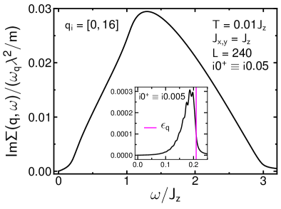
Figure 1: Imaginary part, $\mathrm{Im}\Sigma({\bf q},\omega{+}i0^{+})$ of phonon self-energy versus $\omega$ at fixed small ${\bf q}$, for low $T=0.01J_{z}\lesssim T^{\star}$, using Eq. (14) for homogeneous ground state gauge. Momentum ${\bf q}=2\pi/L\sum_{j=1,2}q_{ij}{\bf G}_{j}$. Inset: Blow up of low-$\omega$ region with reduced imaginary broadening. Magenta line: upper ph-continuum bound at $T=0$.

As a final step, $\Sigma_{\mu\nu}({\bf q},z)$ from Eq. (18) is averaged over a sufficiently large number of random distributions $\{\eta_{{\bf l}}\}$. This concludes the formal details of the evaluation of the self-energy for $T\gtrsim T^{\star}$.

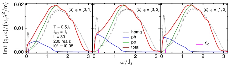
Figure 2: Solid lines: Imaginary part, $\mathrm{Im}\Sigma({\bf q},\omega+i0^{+})$ of phonon self-energy at $T=0.5J_{z}\gtrsim T^{\star}$ versus $\omega$ for three fixed small momenta ${\bf q}=2\pi/L\sum_{j=1,2}q_{ij}{\bf G}_{j}$, i.e. panels (a), (b), (c), using Eq. (18) for random gauge state. Red, green, blue: total, ph, pp spectrum. Gray dashed dotted line: $\mathrm{Im}\Sigma({\bf q},\omega+i0^{+})$ for identical system parameters, however assuming homegeous ground state gauge. Magenta line: upper ph-continuum bound at $T=0$.

IV Results

In this section we discuss selected properties of the phonon self-energy. Ahead of that, several issues have to be addressed. First, we note that material-specific analysis of phonons and a classification of related (pseudo)-spin-phonon coupling processes in potential Kitaev compounds has only begun recently. Most noteworthy, ab-initio calculations suggest that acoustic phonons in $\alpha$-RuCl₃ have sound velocities very similar to those of the fermions at the Dirac coneWidmann2019 ; privateValenti2019 . In view of this, we use a very simple phonon dispersion $\omega_{{\bf q}}=v_{p}[3-\cos(q_{x})-2\cos(q_{x}/2)\cos(\sqrt{3}q_{y}/2)]^{1/2}$, meant solely to show some arbitrarily chosen form of sixfold symmetry and we set $v_{p}\equiv 1$, i.e. of $O(J_{x,y,z})$ hereafter. We emphasize that $\omega_{{\bf q}}$ is simply a scale factor to $\Sigma_{\mu\nu}({\bf q},z)$ with only $\omega_{{\bf q}}\sim O({\bf q})$ at small ${\bf q}$ being relevant for proper hydrodynamic behavior. Second, although $\Sigma_{\mu\nu}(q,i\omega_{n})$ is non-diagonal in principle, such mixing of different phonon branches, is not expected to provide additional qualitative insight. Therefore, for the remainder of this section we focus on a diagonal component $\Sigma({\bf q},z)\equiv\Sigma_{\mu\mu}({\bf q},z)$ of the self-energy, and we furthermore assume the corresponding polarization $\mu$ to be longitudinal. In any material-specific context, the meaning of the latter may be intricateprivateValenti2019 . Here we set ${\bf P}$ to be a unit vector along ${\bf q}$. Third, all result for $\Sigma({\bf q},z)$ are displayed in terms of $\Sigma({\bf q},z)/\omega_{{\bf q}}$, which, in view of the Dyson equation for the phonons is the dimensionless renormalization parameter of the phonon dispersion, i.e. $\omega_{{\bf q}}\rightarrow\omega_{{\bf q}}(1+\Sigma({\bf q},z)/\omega_{{\bf q}})$. Moreover $\Sigma({\bf q},z)/\omega_{{\bf q}}$ is presented on a scale of $\lambda^{2}/m$. The latter quantity encodes the strength of the magnetoelastic coupling. For cuprates with simple spin super-exchange, estimates of the latter existChernyshev2015 . For SOC assisted Mott-insulators with pseudo-spin compass exchange of the Kitaev type, this is an open issue and not part of our analysis. Fourth, we confine the discussion to the imaginary part of $\Sigma({\bf q},\omega+i0^{+})$. This is no loss of information, because of the Kramers-Kronig relation. Fifth, performing the average over gauge configurations in Eq. (18), we use an additional averaging, namely over periodic and antiperiodic boundary conditions. This reduces finite size effects. Sixth and conceptually important, our results for $\mathrm{Im}\Sigma({\bf q},\omega+i0^{+})$ are sixfold symmetric regarding the direction of ${\bf q}$. This seems clear from the original spin hamiltonian and is obviously satisfied in the homogeneous gauge. However also for $T\gtrsim T^{\star}$, with random gauge links along the $z$-bonds, and for all momenta ${\bf q}$ considered, we find that $\mathrm{Im}\Sigma({\bf q},\omega+i0^{+})$ obeys this symmetry.

Now we consider the low-$T$ behavior, using the homogeneous gauge ground state. A typical small-${\bf q}$ spectrum of $\Sigma({\bf q},\omega{+}i0^{+})$ is shown in Fig. 1. From Eq. (14), it comprises two decay types for the phonon, (i) a particle-hole (ph) and (ii) a two-particle (pp) channel. On the scale of the plot only the latter is visible. The inset refers to the ph-channel. In stark contrast to usual phonon-electron scattering, the Fermi volume shrinks to zero in the Kitaev model as $T{\rightarrow}0$, i.e., occupied states only stem from a small patch with $\epsilon_{{\bf k}}\lesssim T$ around the Dirac cone. Therefore, the weight of the ph-channel decreases rapidly to zero as $T{\rightarrow}0$. In this regime and for small-${\bf q}$, because of the linear fermion dispersion close to the cones, the spectral support of the ph-continuum is roughly confined to a narrow strip of order $\omega\in[\max(0,\epsilon_{{\bf q}}-2T),\epsilon_{{\bf q}}]$. At the upper edge of this continuum the ph DOS is singular. The inset of Fig. 1 is consistent with this, considering the finite system size and imaginary broadening used. Regarding the pp-channel, the complete two-particle continuum is unoccupied and available for intermediate states as $T{\rightarrow}0$. This leads to the broad spectral hump seen in Fig. 1, which extends out to $\max(2\epsilon_{{\bf k}})=3J_{z}$, at $J_{x,y}=J_{z}$ and is two orders of magnitude larger than the ph-process at this temperature.

We note that for systems with small-${\bf q}$ phonon velocities, comparable to those of the fermions at the Dirac cone, the on-shell phonon damping $\mathrm{Im}\Sigma({\bf q},\omega_{{\bf q}}{+}i0^{+})$ stems from an energy range similar to that of the inset in Fig. 1. In view of the strong suppression of the ph-channel, the low-$T$ phonon damping, if due to scattering from mobile matter fermions, would primarily result from two-particle decay.

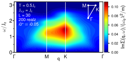
Figure 3: Contours of the imaginary part $\mathrm{Im}\Sigma({\bf q},\omega+i0^{+})$ of the phonon self-energy at $T=0.5J_{z}\gtrsim T^{\star}$ in the random gauge state versus ${\bf q},\omega$ along the path $\Gamma$-$M$-$K$-$\Gamma$ of the BZ.

Next we focus on temperatures above the flux proliferation, i.e. $T\gtrsim T^{\star}$, using a random gauge state. Fig. 2 show the spectrum of $\Sigma({\bf q},\omega{+}i0^{+})$ for three representative low-${\bf q}$ values versus $\omega$. Decomposing Eq. (18) into addends with $\epsilon_{\sigma}\epsilon_{\rho}\gtrless 0$ the ph- and pp-contributions to $\mathrm{Im}\Sigma({\bf q},\omega{+}i0^{+})$ can be extracted and are also shown. For comparison, the spectrum for completely identical system parameters, however in the absence of gauge disorder, i.e. for a homogeneous ground state gauge is included. Small oscillations in the latter are due to larger finite size effects within the homogeneous gauge. Fig. 2 highlights the drastic impact of thermally excited fluxes. While quantitatively, keeping a homogeneous gauge, elevated temperatures merely increase the weight of the ph-channel, qualitatively the latter remains a narrow structure below ${\sim}\epsilon_{{\bf q}}$ in the small-${\bf q}$ limit. This situation changes completely in the thermally excited gauge background. As is obvious from the figure, the ph-channel spreads into a broad feature, extending over roughly the entire one-particle energy range. The shape of this feature is modulated by ${\bf q}$. The pp-channel on the other hand seems less affected by the gauge disorder, with a shape qualitatively similar to that in the gauge ground state.

Interestingly, these findings bear some resemblance to studies of the dynamical thermal conductivity $\kappa(\omega)$ in Kitaev spin systemsMetavitsiadis2017 . While this is a completely different ${\bf q}=0$ correlation function, it also displays a sharp low frequency structure, the so-called Drude-peak $\sim\delta(\omega)$ and a pp-continuum in the homogeneous gauge. However for $T\gtrsim T^{\star}$ the Drude peak is smeared over an energy range $\sim J_{x,y,z}$ by fermions scattering from thermally excited gauges, while the pp-continuum is less affected. Here, Fig. 2 signals a small systematic reduction of the fermion band-width for $T\gtrsim T^{\star}$. Again, the same effect is found in $\kappa(\omega)$.

In Fig. 3 the spectrum of the phonon self-energy is displayed along a path connecting high-symmetry points in the BZ for $T\gtrsim T^{\star}$. This figure has to be taken with a grain of salt. As has been emphasized, Eq. (3) is an approximation for the long wave-length limit, neglecting the two-site basis of the honeycomb lattice regarding the phonons. Therefore the large-${\bf q}$ spectra in Fig. 3 are approximate only. Our main point however, should remain unaffected by this. Namely, that while the two distinct types of relaxation channels, i.e. ph and pp, contained in the low-$T$ limit Eq. (14) and the sharp ph-spike in the spectra assuming a homogeneous gauge, might suggest that $\mathrm{Im}\Sigma({\bf q},\omega{+}i0^{+})$ should display a dispersive feature, shadowing the fermion dispersion, this is not so. On the contrary, for $T\gtrsim T^{\star}$ and because of thermally excited gauges $\mathrm{Im}\Sigma({\bf q},\omega{+}i0^{+})$ in Fig. 3 is almost featureless, covering all of the energy range $\omega\in[0,\max(2\epsilon_{{\bf k}})]$ at any momentum. At low-${\bf q}$, remnants of the fermion ph-continuum boundary can be observed dispersing upwards, however this is only a weak phenomenon. For ${\bf q}$ approaching the $M$ and $K$ points there is a global intensity increase. The role of the small-${\bf q}$ approximation for this is unclear. Finally, for $T\lesssim T^{\star}$ the spectrum is also weakly dispersive only, because of the strong suppression of the ph-channel, as discussed in Fig. 1.

Finally we turn to the temperature dependence of the phonon lifetime. This requires realistic dispersions $\omega_{{\bf q}}$ and values for $\lambda^{2}/m$ to either solve for $z^{2}-\omega_{{\bf q}}^{2}-2\omega_{{\bf q}}\Sigma({\bf q},z)=0$ self consistently, or approximately use the on-shell self-energy $\mathrm{Im}\Sigma({\bf q},\omega_{{\bf q}}{+}i0^{+})$. Lacking this information, we nevertheless consider the latter quantity for fixed values of ${\bf q},\omega$ using three potentially ’typical’ acoustic phonon energies $\omega$ for the chosen low-${\bf q}$ wave vector. This is shown in Fig. 4. The figure highlights two points. First, the qualitative variations of the phonon lifetime with $T$ strongly depends on the actual phonon energy. Second, and universally, since the phonons scatter off a reservoir of fermions, they will undress as the latter turns classical, i.e. as $T\gg J_{x,y,z}$. Since $J_{x,y,z}$ in several Kitaev materials can be of order of the Debye energy, this may be of experimental relevance.

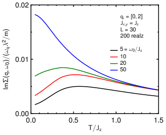
Figure 4: $\mathrm{Im}\Sigma({\bf q},\omega_{0}+i0^{+})$ versus $T$ for fixed momentum ${\bf q}=2\pi/L\sum_{j=1,2}q_{ij}{\bf G}_{j}$ and four energies $\omega_{0}$, using a random gauge state and $T\geqslant 0.05J_{z}$.

V Summary

In conclusion, phonons in Kitaev magnets experience scattering from a characteristic continuum of excitations comprising fractionalized fermionic quasiparticles, allowing for ph- as well as pp-decay channels. In contrast to conventional phonon-electron coupling, thermally excited random gauge fluxes strongly broaden the low-energy ph-channel and render the scattering only weakly dispersive. Our study remains with several open questions. These include a more realistic treatment of the phonon polarizations and band structure, a microscopic analysis of the strength of the magnetoelatic coupling, and related to that, the role of vertex corrections. Moreover, other types of phonon-(pseudo)spin interactions should be considered. Finally, regarding the impact of non-Kitaev exchange, it is tempting to speculate, that similar to previous analysis of transportMetavitsiadis2019a , the pp-decay channel will persist to signal remnants of Majorana physics in the phonon renormalization, even if a sizable Heisenberg exchange is added to the model.

Acknowledgments: We thank R. Valenti and C. Hess for discussion, moreover we are grateful to R. Valenti and S. Biswas for providing us with visualization dataprivateValenti2019 of lattice vibrations in $\alpha$-RuCl₃. Work of W.B. has been supported in part by the DFG through project A02 of SFB 1143 (project-id 247310070), by Nds. QUANOMET, and the NTH-School CiN. W.B. also acknowledges kind hospitality of the PSM, Dresden. This research was supported in part by the National Science Foundation under Grant No. NSF PHY-1748958.

References

- (1) L. Balents, Nature 464, 199-208 (2010).
- (2) L. Savary and L. Balents, Rep. Prog. Phys. 80, 016502 (2017).
- (3) A. Kitaev, Ann. Phys. (N.Y.) 321, 2 (2006).
- (4) X.-Y. Feng, G.-M. Zhang, and T. Xiang, Phys. Rev. Lett. 98, 087204 (2007).
- (5) H.-D. Chen and Z. Nussinov, J. Phys. A: Math. Theor. 41, 075001 (2008).
- (6) Z. Nussinov and G. Ortiz, Phys. Rev. B 79, 214440 (2009).
- (7) S. Mandal, R. Shankar and G. Baskaran, J. Phys. A: Math. Theor. 45, 335304 (2012).
- (8) G. Khaliullin, Prog. Theor. Phys. Suppl. 160, 155 (2005).
- (9) G. Jackeli and G. Khaliullin, Phys. Rev. Lett. 102, 017205 (2009).
- (10) J. Chaloupka, G. Jackeli, and G. Khaliullin Phys. Rev. Lett. 105 027204 (2010).
- (11) Z. Nussinov and J. van den Brink, Rev. Mod. Phys. 87, 1 (2015).
- (12) S. Trebst, Kitaev Materials, Lecture Notes of the 48th IFF Spring School 2017, S. Blügel, Y. Mokrousov, T. Schäpers, Y. Ando (Eds.), ISBN 978-3-95806-202-3
- (13) A. Banerjee, C. A. Bridges, J. Q. Yan, A. A. Aczel, L. Li, M. B. Stone, G. E. Granroth, M. D. Lumsden, Y. Yiu, J. Knolle, S. Bhattacharjee, D. L. Kovrizhin, R. Moessner, D. A. Tennant, D. G. Mandrus, and S. E. Nagler, Nat. Mater. 15, 733 (2016).
- (14) A. Banerjee, J. Yan, J. Knolle, C. A. Bridges, M. B. Stone, M. D. Lumsden, D. G. Mandrus, D. A. Tennant, R. Moessner, and S. E. Nagler, Science 356, 6342 (2017).
- (15) A. Banerjee, P. Lampen-Kelley, J. Knolle, C. Balz, A. A. Aczel, B. Winn, Y. Liu, D. Pajerowski, J. Yan, C. A. Bridges, A. T. Savici, B. C. Chakoumakos, M. D. Lumsden, D. A. Tennant, R. Moessner, D. G. Mandrus, and S. E. Nagler, Nat. Part. J. Quantum Mater. 3, 8 (2018).
- (16) J. Knolle, G.W. Chern, D.L. Kovrizhin, R. Moessner, and N.B. Perkins, Phys. Rev. Lett. 113, 187201 (2014).
- (17) S.-H. Baek, S.-H. Do, K. Y. Choi, Y.S. Kwon, A.U.B. Wolter, S. Nishimoto, J. van den Brink, and B. Büchner, Phys. Rev. Lett. 119, 037201 (2017).
- (18) J. Zheng, K. Ran, T. Li, J. Wang, P. Wang, B. Liu, Z.-X. Liu, B. Normand, J. Wen, and W. Yu, Phys. Rev. Lett. 119, 227208 (2017).
- (19) K. W. Plumb, J. P. Clancy, L. J. Sandilands, V. V. Shankar, Y. F. Hu, K. S. Burch, H.-Y. Kee, and Y.-J. Kim, Phys. Rev. B 90, 041112 (2014).
- (20) Y. Kasahara, T. Ohnishi, Y. Mizukami, O. Tanaka, S. Ma, K. Sugii, N. Kurita, H. Tanaka, J. Nasu, Y. Motome, T. Shibauchi, and Y. Matsuda, Nature 559, 227 (2018).
- (21) J. Cookmeyer, and J. E. Moore, Phys. Rev. B 98, 060412(R) (2018).
- (22) P. A. McClarty, X. -Y. Dong, M. Gohlke, J. G. Rau, F. Pollmann, R. Moessner, and K. Penc, Phys. Rev. B 98, 060404(R) (2018).
- (23) M. Ye, G. B. Halász, L. Savary, and L. Balents, Phys. Rev. Lett. 121, 147201 (2018).
- (24) Y. Vinkler-Aviv, and A. Rosch, Phys. Rev. X 8, 031032 (2018).
- (25) D. Hirobe, M. Sato, Y. Shiomi, H. Tanaka, and E. Saitoh, Phys. Rev.~B 95, 241112 (2017).
- (26) I.A. Leahy, C.A. Pocs, P.E. Siegfried, D. Graf, S.-H. Do, K.-Y. Choi, B. Normand, and M. Lee, Phys. Rev. Lett. 118, 187203 (2017).
- (27) R. Hentrich, A. U. B. Wolter, X. Zotos, W. Brenig, D. Nowak, A. Isaeva, T. Doert, A. Banerjee, P. Lampen-Kelley, D. G. Mandrus, S. E. Nagler, J. Sears, Y.-J. Kim, B. Büchner, C. Hess, Phys. Rev. Lett. 120, 117204 (2018).
- (28) Y. J. Yu, Y. Xu, K. J. Ran, J. M. Ni, Y. Y. Huang, J. H. Wang, J. S. Wen, and A. Y. Li, Phys. Rev. Lett. 120, 067202 (2018).
- (29) A. Glamazda, P. Lemmens, S.-H. Do, Y. S. Kwon, and K.-Y. Choi, Phys. Rev. B 95, 174429 (2017).
- (30) A. Sahasrabudhe, D. A. S. Kaib, S. Reschke, R. German, T. C. Koethe, J. Buhot, D. Kamenskyi, C. Hickey, P. Becker, V. Tsurkan, A. Loidl, S. H. Do, K. Y. Choi, M. Grüninger, S. M. Winter, Z. Wang, R. Valenti, and P. H. M. van Loosdrecht, ArXiv:1908.11617 [Cond-Mat] (2019).
- (31) S. Reschke, V. Tsurkan, S.-H. Do, K.-Y. Choi, P. Lunkenheimer, Z. Wang, and A. Loidl, Phys. Rev. B 100, 100403(R) (2019).
- (32) S. Widmann, V. Tsurkan, D. A. Prishchenko, V. G. Mazurenko, A. A. Tsirlin, and A. Loidl, Phys. Rev. B 99, 094415 (2019).
- (33) T. Biesner, S. Biswas, W. Li, Y. Saito, A. Pustogow, M. Altmeyer, A. U. B. Wolter, B. Büchner, M. Roslova, T. Doert, S. M. Winter, R. Valentí, and M. Dressel, Phys. Rev. B 97, 220401 (2018).
- (34) G. Bastien, G. Garbarino, R. Yadav, F. J. Martinez-Casado, R. Beltrán Rodríguez, Q. Stahl, M. Kusch, S. P. Limandri, R. Ray, P. Lampen-Kelley, D. G. Mandrus, S. E. Nagler, M. Roslova, A. Isaeva, T. Doert, L. Hozoi, A. U. B. Wolter, B. Büchner, J. Geck, and J. van den Brink, Phys. Rev. B 97, 241108 (2018).
- (35) R. Yadav, S. Rachel, L. Hozoi, J. van den Brink, and G. Jackeli, Phys. Rev. B 98, 121107 (2018).
- (36) G. L. Stamokostas, P. E. Lapas, and G. A. Fiete, Phys. Rev. B 95, 064410 (2017).
- (37) J. Nasu, M. Udagawa, and Y. Motome, Phys. Rev. B 92, 115122 (2015).
- (38) A. Metavitsiadis, A. Pidatella, and W. Brenig, Phys. Rev. B 96, 205121 (2017).
- (39) A. Pidatella, A. Metavitsiadis, and W. Brenig Phys. Rev. B 99, 075141 (2019).
- (40) A. Metavitsiadis and W. Brenig, Rev. B 96, 041115(R) (2017).
- (41) A. A. Abrikosov, L. P. Gorkov, and I. E. Dzyaloshinski, Methods of Quantum Field Theory in Statistical Physics, Dover Publications Inc., ISBN 0486140156
- (42) A. B. Migdal, Sov. Phys. JETP 7, 996 (1958).
- (43) B. Roy, J. D. Sau, and S. Das Sarma, Phys. Rev. B 89, 165119 (2014).
- (44) A. L. Chernyshev and W. Brenig, Phys. Rev. B 92, 054409 (2015).
- (45) R. Valenti, S Biswas, private communication, unpublished
- (46) A. Metavitsiadis, C. Psaroudaki, and W. Brenig, Phys. Rev. B 99, 205129 (2019).