Exclusivity graph approach to Instrumental inequalities

Abstract

Instrumental variables allow the estimation of cause and effect relations even in presence of unobserved latent factors, thus providing a powerful tool for any science wherein causal inference plays an important role. More recently, the instrumental scenario has also attracted increasing attention in quantum physics, since it is related to the seminal Bell’s theorem and in fact allows the detection of even stronger quantum effects, thus enhancing our current capabilities to process information and becoming a valuable tool in quantum cryptography. In this work, we further explore this bridge between causality and quantum theory and apply a technique, originally developed in the field of quantum foundations, to express the constraints implied by causal relations in the language of graph theory. This new approach can be applied to any causal model containing a latent variable. Here, by focusing on the instrumental scenario, it allows us to easily reproduce known results as well as obtain new ones and gain new insights on the connections and differences between the instrumental and the Bell scenarios.

1 INTRODUCTION

Inferring whether a variable $A$ is the cause of another variable $B$ is at the core of causal inference [1]. However, unless interventions are available [2], one can cannot exclude that observed correlations between $A$ and $B$ are due to a latent common factor, thus hindering any causal conclusions. To cope with that, instrumental variables (IV) have been introduced [3, 4]. Under the assumption that they are independent of any latent common factors $\Lambda$, IV can be used to put non-trivial bounds on the causal effect between $A$ and $B$. However, first, one has to guarantee that an appropriate instrument (fulfilling a set of causal constraints) has been employed, which is precisely the goal of the so-called instrumental tests [3, 4, 6, 7]. Their violation, at least in classical physics, is an unambiguous proof that some of the causal assumptions underlying the instrumental causal structure are not fulfilled, that is, one should identify and use another instrumental variable.

Instrumental tests have firstly been introduced in econometrics [5] and further explored by Pearl [3], in the form of inequalities providing a necessary condition for a given observed probability distribution to be compatible with the instrumental causal structure. Following that, Bonet [4] introduced a general framework also followed in [6], showing that the instrumental correlations define a polytope, a convex set from which the non-trivial boundaries are precisely the instrumental inequalities. Bonet’s framework allows for the derivation of new inequalities as well as proving general results, for instance, the fact that if variable $A$ is continuous, no instrumental test exists. However, two main drawbacks arise. First, the systematic derivation of new inequalities quickly becomes unfeasible as the variables’ cardinalities increase. Second, as recently shown, in quantum physics, violations of the instrumental tests are possible even though the whole process is indeed subjected to an instrumental causal structure [8, 9]. In the quantum case, instrumentality violations witness the presence of quantum entanglement as the latent factor and prove a stronger form of quantum non-locality compared to the famous Bell’s theorem [8]. As a consequence, typical bounds on the causal influence of $A$ into $B$ have to be reevaluated and reinterpreted in the presence of quantum effects.

Our aim in this paper is to provide a novel and complementary framework to the analysis of instrumental tests, which also addresses the two drawbacks mentioned above. The proposed method is based on a graph theoretical approach introduced in the foundations of quantum physics to analyze the possible correlations obtained in quantum experiments [10, 11]. This method allow us to reproduce the classical results by Bonet and to straightforwardly generalize them in the quantum scenario. It also offers an easy and general way – valid for any causal scenario involving a single latent variable – to check for the incompatibility between the quantum and classical descriptions.

The paper is organized as follows: first we provide the necessary background for our work, describing the instrumental and Bell scenarios from both classical and quantum perspectives and introducing the exclusivity graph approach. We then show the versatily of our framework by rederiving and generalizing known results in the literature, obtaining new instrumental inequalities that hardly could be found by standard means and offering new insights about the similarities and differences between instrumental and Bell inequalities.

Figure 1: Directed acyclic graph (DAG) representation for a) a general Instrumental scenario, with $l$ possible values for the random variable $X$ and $m,n$ possible outcomes for $A$ and $B$ respectively, and for b) the CHSH scenario [12] where all the variables $X,Y,A$ and $B$ can only take two possible values.

2 INSTRUMENTAL VARIABLES, ESTIMATION OF CAUSAL INFLUENCES AND A NEW FORM OF QUANTUM NON-LOCALITY

We represent causal relations via directed acyclic graphs (DAG), where the nodes represent random variables interconnected by directed edges (arrows) accounting for their cause and effect relations [2]. A set of variables $\left(X_{1},\dots,X_{n}\right)$ form a Bayesian network with respect to the graph if every variable $X_{i}$ can be expressed as a function of its parents $\mathrm{PA}_{i}$ and potentially an unobserved noise term $U_{i}$, such that $U_{i}$ are jointly independent. This implies that the probability distribution of such variables should have a Markov decomposition

$$p(x_{1},\dots,x_{n})=\prod_{i=1}^{n}p(x_{i}|\mathrm{pa}_{i}).$$ (1)

Importantly, a DAG typically implies non-trivial constraints over the probability distributions that are compatible with it. That is, simply from observational data and without the need of interventions, one can test whether some observed correlations are incompatible with some causal hypotheses.

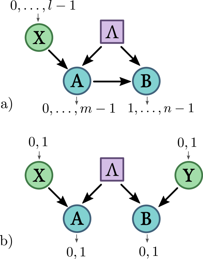
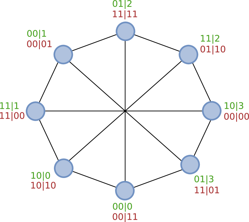
Within this context, an important DAG is that corresponding to the instrumental scenario (see Fig.1-a). Following the Markov decomposition, any empirical data encoded in the probability distribution $p(a,b|x)$ and compatible with the instrumental causal structure can be decomposed as

$$p(a,b|x)=\sum_{\lambda}p(a|x,\lambda)p(b|a,\lambda)p(\lambda).$$ (2)

Two causal assumptions are employed to arrive to the above decomposition. i) The first assumption $p(x,\lambda)=p(x)p(\lambda)$, implies the independence of the instrument and the common ancestor. ii) The second assumption requests that, even though $X$ and $B$ can be correlated, all these correlations are mediated by $A$. In other terms, there is no direct causal influence between $X$ and $B$: $p(b|x,a,\lambda)=p(b|a,\lambda)$.

The instrumental variables have been originally introduced to estimate parameters in econometric models of supply and demand [13] and, since then, have found a wide range of applications in various other fields [14, 15]. To illustrate its power, consider that variables $A$ and $B$ are related by a simple linear equation, i.e. $B=\gamma A+\Lambda$, where $\Lambda$ may represent a latent common factor. By assumption, the instrumental variable $X$ should be independent of $\Lambda$, thus implying that the causal strength can be estimated as $\gamma=\mathrm{Cov}(X,B)/\mathrm{Cov}(X,A)$ where $\mathrm{Cov}(X,A)$ is the covariance between $X$ and $A$. Strikingly, one can estimate the causal strength even without any information about the latent factor $\Lambda$. More generally, and without assumptions about the functional dependence among the variables, the empirical data encoded in the probability distribution $p(a,b|x)$ can also be used to bound different quantifiers of causality between $A$ and $B$ [2, 16].

Clearly, however, to draw any causal conclusions, first it is necessary to certify that one has a valid instrument. This is achieved via instrumental inequalities, first introduced by Pearl [3]. If we allow the variables $X$, $A$, $B$ to take the values in the range $x=1,\dots,l$, $a=1,\dots,m$ and $b=1,\dots,n$ Pearl showed that the instrumental causal structure implies (independently of any assumption about the functional dependence among the variables) that

$$\sum_{j=0}^{n}P(ij|k(i,j))\leq 1,$$ (3)

for all $i\in{1,\ldots,m}$ and for all the possible functions $k(i,j)$ where $p(i,j|k)=p(a=i,b=j|x=k)$.

Extending these results, Bonet [4] provided a general geometric framework for the derivation of instrumental inequalities. Instrumental correlations define a convex set, a polytope described by finitely many extremal points, or alternatively by a finite number of facets, among which, the non-trivial are precisely the instrumental inequalities. In particular, considering the case $(l,m,n)=(3,2,2)$, it was proven that there are two inequivalent classes of instrumental inequalities (those not obtained from each other by permuting the labels of $i,j$ and $k$). One class corresponding to Pearl’s inequality (3) and the other given by

$$P(00|0)+P(11|0)+P(00|1)+\\ +P(10|1)+P(01|2)\leq 2.$$ (4)

All these conclusions and results, however, rely on a classical description of causal and effect relations (implicitly) invoking the realism assumption: the probabilities of a given measurement have well defined values even if such measurements are not performed. However, since Bell’s theorem [17] we know that this do not apply to the world governed by quantum mechanics, thus implying that standard causal models, even if augmented with latent variables, are not enough to explain quantum phenomena. Bell’s theorem relies on the causal structure shown in Fig. 1-b, similar to the instrumental one but with two crucial causal differences: i) variable $A$ has no causal influence over $B$ and ii) $B$ has its own instrument $Y$ and thus the correlations are encoded in a probability distribution $p(ab|xy)$. This has motivated the question of whether many of the cornerstones in causal inference have to be re-evaluated or reinterpreted in the presence of quantum effects [18, 19, 20, 21, 22]. Indeed, as recently shown [8], violations of the instrumental tests are possible even though the causal constraints underlying the instrumental scenario are fulfilled. As shown in the experimental implementation of the instrumental test [8], this is possible due to the presence of quantum entanglement that precludes the explanation of the data via a latent common factor. Interestingly, every probability distribution violating the simplest possible Bell inequality, known as Clauser-Horne-Shimony-Holt (CHSH) inequality [12], can after some post-processing also violate Bonet’s inequality [9]. As we will see, the graph-theoretical approach will allow us a more systematic understanding of the similarities and differences between the Bell and instrumental scenarios.

Altogether, this shows the necessity of a new unifying framework, not only considering what are the classical instrumental correlations but as well the ones achievable if the underlying latent factor might have a quantum origin. In the following we will achieve that by proposing a graph-theoretical approach to analyze the instrumental inequalities.

3 THE EXCLUSIVITY GRAPH APPROACH

The graph-theoretical approach we propose here, was initially developed for the study of non-contextual inequalities [10] as well as Bell non-locality scenarios [23]. The purpose of this method is to easily obtain constraints on the probability distribution, in the same spirit of the Pearl’s and Bonet’s inequalities, for classical and quantum systems. In the following we will have a set of random variables $A_{1},\ldots,A_{N}$ representing the outcomes of measurements performed on our physical system, and another set $X_{1},\ldots,X_{M}$, a number of measurement settings that can be chosen by the experimenter, which serve the same purpose of the instrument in the IV scenario. In the exclusivity graph formalism, every possible event, i.e. every possible set of measurement outcomes $a_{1},\ldots,a_{N}$ corresponding to given measurement settings $x_{1},\ldots,x_{M}$ , is associated to a vertex in a (undirected) graph $G=(V,E)$. Two vertices $u,v\in V$ are connected by an edge $(u,v)\in E$ if and only if they are exclusive, i.e., if there is a measurement/instrument that can distinguish between them. Intuitively, two events are exclusive when they cannot happen simultaneously in the same run of the experiment. For example, in the Bell scenario depicted in Fig. 1-b, events where we get $a=0$ or $a=1$, while setting $x=0$ for both, are exclusive, since only one of them can happen in a single run of the experiment. On the contrary, if the setting $x$ is different (for example $x=1$ for $a=0$ and $x=0$ for $a=1$), the events will not be exclusive since a single experimental test cannot distinguish between them. In the next section we will provide a precise definition of exclusivity which will allow us to extend this concept to a wide range of causal models.

Any linear constraint (like the instrumental inequalities) can be expressed by a linear function

$$I_{w}(p)=\sum_{\begin{subarray}{c}a_{1},\ldots,a_{n}\\ x_{1},\ldots,x_{n}\end{subarray}}w_{\mathbf{a},\mathbf{x}}p(a_{1},\ldots,a_{n}|x_{1},\ldots,x_{n}),$$ (5)

on the probabilities of possible events. This linear function can be embedded in an exclusivity graph by weighting the vertices in $G$ with the $\left\{w_{\mathbf{a},\mathbf{x}}\right\}$, so that it can be written as a function of $G=(V,E)$ and its weights as

$$I(G,w)=\sum_{v\in V}w_{v}p(v).$$ (6)

Nicely, as it will be discussed below, bounds for the maximum values of $I_{w}(p)$, achievable both in the classical and quantum cases, can be related to two well-known graph invariants [10]: the independence number $\alpha(G,w)$ and the Lovász theta $\theta(G,w)$, respectively. In the following, we will briefly introduce these concepts and their interconnections, a more extensive and detailed account can be found in [10, 11, 23]

Consider a graph $G(V,E)$ with vertex weights $w$, and $|V|=n$. We call a characteristic labelling for $U\subseteq V$ a vector $x_{v}\in\{0,1\}^{n}$ such that $x_{v}=1$ if $v\in U$ and $x_{v}=0$ otherwise. An independent set or stable set is a set $S\subset V$ such that $(u,v)\notin E$ for all $u,v\in S$. The independence number $\alpha(G,w)$ is defined as the maximum number of vertices (weighted with $w$) of an independent set of $G$. In the case of exclusivity graphs, any characteristic labelling of a stable set, also called a stable labelling, represents a possible deterministic assignment of probabilities which respects the exclusivity constraints, i.e. such that no exclusive events can be assigned probability one at the same time. It is also customary to define the set $\mathrm{STAB}(G)$ as the convex hull of all the characteristic labellings of stable sets, such that

$$\mathrm{STAB}(G)=\mathrm{Conv}(\{x:\\ x\quad\text{is a stable labelling of}\quad G\}).$$ (7)

Since stable labellings represent all the possible deterministic strategies respecting the exclusivity relations, then $\mathrm{STAB}(G)$ effectively includes all the possible probability assignments compatible with those constraints. Now we can define the independence number as

$$\alpha(G,w)=\max\{w\cdot x:x\in\mathrm{STAB}(G)\}.$$ (8)

Thus, $\alpha(G,w)$ must correspond to the classical bound of the inequality, since it is exactly the maximum over the convex set defined by all the deterministic strategies respecting the exclusivity constraints. Classical models are those described precisely by such convex set, thus implying that

$$I(G,w)\leq\alpha(G,w).$$ (9)

Moreover, the bound is tight since it is saturated by any deterministic assignment corresponding to a maximal stable set.

In associating the set $STAB(G)$ with the space of the possible probability distributions for our graph $G$, we have made the implicit assumption that there exists a joint probability distribution for all of our events, i.e., that even when certain settings are not chosen by the experimenter, we can still assign (counterfactually) a value to their probabilities. This is the realism assumption mentioned above that, as implied by Bell’s theorem, cannot hold true togheter with locality for quantum systems. In the following, we briefly introduce the probabilistic framework used in quantum mechanics, the interested reader can refer to classic texts such as [24]. In quantum mechanics the state of the system, which plays a similar role as the probability distribution for classical systems, is represented by a vector $\Psi$ in a complex Hilbert space $\mathcal{H}$, normalized such that $\left|\Psi\right|^{2}=1$. Likewise, measurements are associated to a set to an orthonormal basis $\{\Phi_{1},\ldots,\Phi_{d}\}$ in the same space $\mathcal{H}$, each associated to a possible measurement outcome . It is also customary to represent measurements using projection operators $E_{i}=\Phi_{i}(\Phi_{i})^{T}$, so that $E_{i}E_{j}=0\,\forall i,j$ and $\sum_{i}E_{i}=I$. The probability associated to each outcome is defined by the Born’s rule:

$$p_{i}=\Psi^{T}E_{i}\Psi=\left|\Psi\cdot\Phi_{i}\right|^{2}.$$ (10)

It is known that such framework allows for a set of probability distributions which is in general larger than the classical one. Exclusivity relations between events (measurement outcomes) in the quantum framework translate into orthogonality between projectors. A quantum realization of an exclusivity graph $G(V,E)$ then consists in a set projectors $E_{i}$ for each vertex $i\in V$, such that $E_{i}$ and $E_{j}$ are orthogonal each time $i$ and $j$ are connected by an edge. This corresponds to what in graph theory is known as an orthonormal labelling of $G$. An orthonormal labelling of dimension $d$ is a map $a_{v}:V\rightarrow\mathbb{R}^{d}$ such that $a_{v}\cdot a_{u}=0$ for all $(u,v)\in E$ and $|a_{v}|^{2}=1$. Using that notion we can define the set $\mathrm{TH}(G)$ as

$$\mathrm{TH}(G)=\{x:x_{v}=(a_{v})_{1}\,\text{where $a_{v}$ is an}\\ \text{orthonormal labelling of $G$}\}.$$ (11)

It can be proved that this set includes all correlations permitted by quantum theory but in general is larger as it contains correlations beyond those achievable by quantum mechanics [25]. Maximizing over $\mathrm{TH}(G)$ led to the Lovász theta given by

$$\theta(G,w)=\max\{w\cdot x:x\in\mathrm{TH}(G)\},$$ (12)

which upper-bounds the maximum quantum value of $I(G,w)$ in equation (6). Despite not being a tight bound for quantum system in general, $\theta(G,w)$ is known to be efficiently computable, by a semi-definite program.

This also provide a useful condition to check if a given graph $G$ (or any of its induced subgraphs) admits a quantum violation. Indeed using a known result of graph theory we know $\mathrm{TH}(G)=\mathrm{STAB}(G)$ if and only if $G$ does not contain a cycle $C_{n}$ with $n\geq 5$ and odd, or its complement as induced subgraphs. This follows directly from the so called sandwich theorem [27, 28] and the strong perfect graph theorem [31]. The first one states that the number $\theta(G)$ is always greater or equal the independence number of the graph $\alpha(G)$.

$$\alpha(G)\leq\theta(G)$$ (13)

When equality holds in equation (13) for a graph $G$ and all its induced subgraphs, $G$ is called perfect. For perfect graphs, we can exclude the existence of a quantum violation, since $\alpha(G)=\theta(G)$. The second theorem then gives a useful condition to check if a graph is perfect or not. In particular it affirms that a graph $G$ is perfect if and only if it does not contain a $n$-cycle graph with $n\geq 5$ and odd or its complement as an induced subgraph. Besides signaling the presence of a possible quantum violation of a classical constraint, induced cycle subgraphs are also interesting because they give the simplest inequalities (in terms of number of probabilities to estimate), to test this violation.

4 EXCLUSIVITY GRAPH METHOD APPLIED TO CAUSAL MODELS

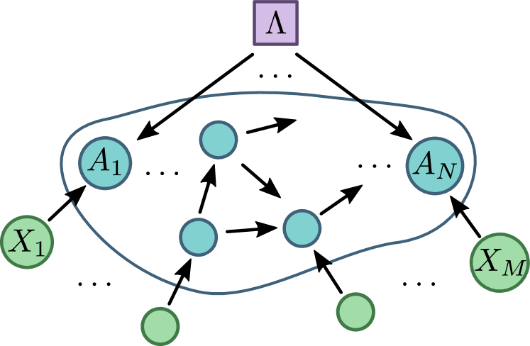
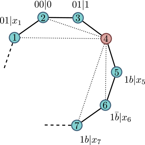
In this section we show how the techniques presented in the previous section can be employed to analyze a broad class of causal models. Consider the DAG depicted in Fig 2, with $N$ observable variables $A_{1},\ldots,A_{N}$ with arbitrary causal arrows among them, $M$ instruments $X_{1},\ldots,X_{M}$, and a single unobservable latent variable $\Lambda$ acting as a potential common factor for all $A_{i}$s (but not for the $X_{j}$s).

Figure 2: Represetantion of the class of causal structures to which our method can be applied, which are those with $k$ observable variables, $l$ instruments and a single latent variable.

An exclusivity graph can be associated with such a DAG as follows:

• Nodes are associated to events like $a|x$, where $a=(a_{1},\ldots,a_{N})$ and $x=(x_{1},\ldots,x_{M})$.

• Two nodes $a|x$, and $a^{\prime}|x^{\prime}$ are linked by an edge if there is at least a variable $A_{i}$ for which does not exists any function $f_{i}$ such that:

  $$f_{i}(\mathrm{pa}_{i})=a_{i}\;\mathrm{and}\;f_{i}(\mathrm{pa}_{i}^{\prime})=a^{\prime}_{i}.$$ (14)

  where $\mathrm{pa}_{i}$ and $\mathrm{pa}_{i}^{\prime}$ represent the values taken by the parents of $A_{i}$ in the two events.

For example, referring to the Bell scenario of Fig. 1-b any two events $a,b,x,y$ and $a^{\prime},b^{\prime},x^{\prime},y^{\prime}$ where $x=x^{\prime}$ and $a\neq a^{\prime}$ (or $y=y^{\prime}$ and $b\neq b^{\prime}$) are exclusive, since we would need $f(x)\neq f(x^{\prime})$ even if $x=x^{\prime}$ (or similarly $g(y)\neq g(y^{\prime})$ when $y=y^{\prime}$). As we will show next, considering the particular case of the instrumental scenario [3, 4], one can apply the graph-theoretical methods delineated before to its corresponding exclusivity graph, $G$, and its induced subgraphs. This allows to obtain instrumental inequalities and their respective quantum and classical bounds. To do that, we proceed as follows: First we try to determine if the graph is perfect using the strong perfect graph theorem, i.e. looking for odd cycles and anticycles with more than $5$ vertices among the induced subgraphs of $G$. If the graph is perfect, then we know immediately that no quantum violation is possible. If the graph is not perfect, then we must have found some odd cycle or anticycle $C_{n}$. These kinds of induced subgraphs represent our minimal candidates for a quantum violation, cause we already know that for them $\alpha(C_{n})<\theta(C_{n})$, in particular:

$$\alpha(C_{n}) =\lfloor n/2\rfloor$$ (15)

$$\theta(C_{n}) =\frac{n\cos(\pi/n)}{1+\cos(\pi/n)}$$

Other candidates can be found among the induced subgraphs of $G$, possibily with non-unitary weights $w$, which contain at least one of those cycles/anticycles. So any weighted subgraph $S$ that satisfies $\alpha(G,w)<\theta(G,w)$ in the end must contain at least a unitary weighted subgraph with this same property. For this reason in the following analysis we focus on cycles or on unitary weighted graphs only.

4.1 THE INSTRUMENTAL EXCLUSIVITY GRAPH

Figure 3: The exclusivity graph for the instrumental scenario with $m=n=2$ and $l=2,3,4,5$ respectively from top left to bottom right. To simplify the representation cliques are represented with the bold lines in the figure.

As a first application we will restrict our attention to the instrumental scenario in the case of dichotomic measurements ($n=m=2$). We denote the probability of having outcomes $a$ and $b$ with the instrument assuming the value $x$ as $p(ab|x)$ with $a,b\in\mathcal{A}=\mathcal{B}=\{0,1\}$ and $x\in\mathcal{X}=\{0,\ldots,l\}$. As explained above, the exclusivity graph for the instrumental scenario is obtained by connecting two events $a,b,x$ and $a^{\prime},b^{\prime},x^{\prime}$ with an edge if we cannot find a function $f:\mathcal{X}\rightarrow\mathcal{A}$ such that:

$$a=f(x)\quad\text{and}\quad a^{\prime}=f(x^{\prime})$$ (16)

or a function $g:\mathcal{A}\rightarrow\mathcal{B}$ such that:

$$b=g(a)\quad\text{and}\quad b^{\prime}=g(a^{\prime})$$ (17)

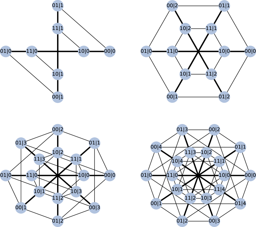
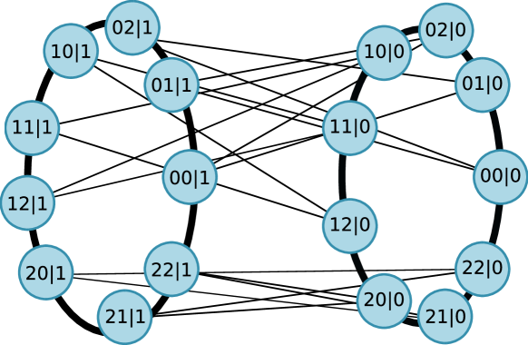
Using these rules we construct the exclusivity graphs $G_{l}=(V_{l},E_{l})$ for various $l$, some of which are shown in Fig. 3, and use the methods described in the previous sections to obtain the classical and quantum bounds for several inequalities in the instrumental scenario.

First, consider the case $l=2$, depicted in Fig. 3 top-left, for which Pearl’s inequality (3) defines the only instrumental inequality. It has been shown that this inequality does not have a quantum violation [29]. For that, general probabilistic Bayesian networks, including classical and quantum causal models as particular cases, had to be introduced. In contrast, in our method it is straightforward not only to derive the classical bound to Pearl’s inequality but also show that there is no quantum violation of the inequality. In the case of $l=2$ inequalities (3) becomes:

$$P(a0|x)+P(a1|x^{\prime})\leq 1\,\forall a,x,x^{\prime}\in\{0,1\}$$ (18)

which are just the classical constraint given by the exclusivity conditions represented by the edges of the graph (see Fig. 3). Indeed considering the trivial induced subgraphs $S_{e}$ formed by only two vertices $e=(v_{1},v_{2})\in E_{2}$, we simply have $\alpha(S_{e})=1$ from which using equation (9), we obtain contraints in (18). The fact that no quantum violation is allowed follows immediately from the fact that the corresponding exclusivity graph (and its complement) does not contain any odd cycle or anticycle with more than $5$ vertices, which makes it a perfect graph, i.e. $TH(G)=STAB(G)$. This can be easily proved in the case $l=2$ for any number of outputs $n,m$ as shown in the supplemental materials. In this way we can exclude the presence of any quantum violation for any scenario where the instrument can only take two possible values ($l=2$) and an arbitrary number of outputs for $A,B$.

Figure 4: The exclusivity graph of the bonet inequality as an induced subgraph of complete one of the $(l,m,n)=(4,2,2)$ instrumental scenario. To simplify the representation, cliques are represented with the bold lines in the figure.

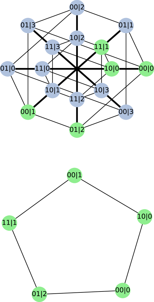
Going to higher number of outcomes for the instrument $X$ we see that there might be a quantum violation, since the associated graph $G_{l}$ has as a $C_{5}$ cyclic graph as induced subgraph for $l\geq 3$. The graph $C_{5}$, depicted in Fig. 4, represents an instance of Bonet’s inequality (4), and indeed from equation (15) we get the expected classical bound $\alpha(C_{5})=2$. The quantum limit, as already mentioned, in general does not saturate the bound given by $\theta(G)$, which in this case is (from (15)) $\theta(C_{n})=\sqrt{(}5)$. To find a tighter bound we can apply the technique described in [11], which is in turn based on the so called NPA method (from M. Navascués, S. Pironio, A. Acín) described in [26]. This is a method commonly employed in quantum information to perform optimizations constrained in the set of quantum correlations. Since, in general, there are no known methods to impose this exact optimization condition, the technique works by relaxing the problem to a, virtually infinite, hierarchy of semi-definite programs of increasing dimension, which approximate the restriction to quantum correlations. Applying it to Bonet inequality we are able obtain the known result for the maximum quantum bound, i.e $(3+\sqrt{2})/2\approx 2.2071$ (more details can be found in the supplemental materials).

As shown in the supplemental material, no other odd cycle besides $C_{5}$ is present for any $l$, that is, if we increase the cardinality of the instrumental variable. The first $7$-cycle appears as soon as we get to $n=m=3$ and $l=4$. An instance of this Bonet-like inequality for the instrumental scenario can be written as:

$$P(00|2)+P(02|3)+P(00|0)+P(12|0)+\\ +P(10|1)+P(21|1)+P(22|2)\leq 3$$ (19)

Applying the method cited above for this inequality gives a quantum upper bound of $q=3.2990$ at the second order of the hierarchy, which indicates the possibility of a quantum violation. Similarly, numerical analysis shows that odd cycle subgraphs with higher number of vertices appear only if we increase the number of possible settings $l$ while also increasing $m$, so for example $9$-cycles start to appear for $l=6,m=3$ and $11$-cycles for $l=7,m=4$.

Figure 5: Exclusivity graphs for the the inequality (21) in the Bell scenario (in red) and inequality (20) in the instrumental scenario (in green).

While cycles are the simplest inequalities showing quantum violation, our method can also be employed for the analysis of different inequalities, that can be devised by other choices of vertices. For example in the instrumental scenario $(l,m,n)=(4,2,2)$ we can find by inspection the inequality:

$$P(01|2)+P(11|2)+P(10|3)+P(01|3)+\\ +P(00|0)+P(10|0)+P(11|1)+P(00|1)\leq 3$$ (20)

This inequality is interesting, since it is represented by the same exclusivity graph of the notorious CHSH inequality [12] for the Bell scenario (see Fig. 5):

$$P(00|00)+P(11|00)+P(00|01)+P(11|01)+\\ +P(01|10)+P(10|10)+P(00|11)+P(11|11)\leq 3$$ (21)

A well known generalization of the CHSH inequality are the so called CGLMP (Collins, Gisin, Linden, Massar and Popescu) inequalities, introduced in [30], which are defined for any Bell scenario with 2 settings for $X$ and $Y$ and $d$ outcomes for $A$ and $B$, and can be written as:

$$I_{d}^{\mathrm{CGLMP}}=\sum_{k=0}^{d-1}(d-1-k)S^{d}_{k}\leq 3(d-1)$$ (22)

where

$$\quad S^{d}_{k}=\sum_{b}(P(b+k,b|00)+P(b+k,b|11))+$$ (23)

$$+\sum_{a}(P(a,a+k+1|10)+P(a,a+k|01))$$

where the sums $a+k,a+k+1$ and $b+k$ are modulo $d$. Using the exclusivity graph method we can find that each of the $S^{d}_{k}$ is classically constrained by:

• $\alpha(G^{d}_{k})=4$ if $k$ and $d$ satisfy $4k+1=nd$, for some integer $n$.

• $\alpha(G^{d}_{k})=3$ in the other cases.

Indeed the graphs $G^{d}_{k}$ relative to the $k$ all share the same structure: there are four cliques, one for each setting $x,y\in\{0,1\}$, and any vertex in each clique is connected to every other vertex in the adjacent clique, except for one. For example $P(b+k,b|00)$ is connected to any node belonging to the $(0,1)$ and the $(1,0)$ cliques, except for $P(a,a+k|01)$ and $P(a^{\prime},a^{\prime}+k+1|10)$ where $b+k=a$ and $a^{\prime}+k+1=b$. Clearly a maximal independent set cannot contain more than $4$ vertices (one for each clique). Moreover to be an independent set, a set of four nodes $\{P(b+k,b|00),P(b^{\prime}+k,b^{\prime}|11),P(a,a+k|01),P(a^{\prime},a;+k+1|01)\}$ must satisfy the conditions:

$$\left\{\begin{aligned} &b+k=a\\ &a+k=b^{\prime}\\ &b^{\prime}+k=a^{\prime}\\ &a^{\prime}+k+1=b\end{aligned}\right.$$ (24)

where the sums are all modulo $d$. From this follows directly that $4k+1=0$.

To obtain the quantum bounds we can apply the same method discussed above. The results for some $S_{k}$ inequalities are shown in Table 1.

$d$	$k$	$\alpha(G^{d}_{k})$	$\theta(G^{d}_{k})$	NPA
3	0	3	3.464	3.333
3	1	3	3.464	3.333
4	0	3	3.414	3.307
4	1	3	3.414	3.307
5	0	3	3.431	3.294
5	1	4	3.999	3.999

Table 1: Considering the inequality $S^{d}_{k}$ for different values of $k$ and $d$, the table above shows the independence number $\alpha(G^{d}_{k})$, the Lovász theta $\theta(G^{d}_{k})$ and the NPA bound computed up to the second order of the hierarchy.

Interestingly, except for the case $(l,m,n)=(4,2,2)$, inequalities with the same structure do not seem to arise in the instrumental case, which suggests that the apparent similarity noticed in [9] between the two scenarios, Bell and the instrumental, only appears for specific number of inputs and outputs.

5 DISCUSSION

In this paper, we have proposed an unifying formalism to analyze classical and quantum correlations arising in a broad class of causal structures. It is based on a graph-theoretical formalism originally introduced in the field of quantum information [10, 11, 23]. In particular, we consider the application of this formalism to analyze instrumental tests [3]. As we show, the probabilities arising in such experiments can be encoded in a exclusivity graph and from there it follows that the classical and quantum bounds respected by instrumental inequalities are related to two graphs invariants: the independence number, $\alpha$, and Lovász $\theta$, respectively.

Apart from the fundamental relevance of bridging the fields of quantum information and causal inference, our approach is also shown to be of practical use. We not only re-derived, in an easy manner, previous results in the literature, we also manage to generalize them. For instance, we prove the inequalities associated with an instrument assuming only two possible values do not have a quantum violation (irrespectively of the number of outcomes), thus generalizing the results in [29]. As well, we prove that if the number of outcomes is fixed to two (the instrument now assuming any cardinality), there are no other inequalities other than the original Bonet’s inequality [4] arising from a n-cycle graph. Following that, we have shown how new instrumental inequalities associated with n-cycles of increasing n can be obtained by increasing the possible values of both the instrument and the outcomes.

The graph approach also constitutes a valuable tool to study similarities among different scenarios and inspect whether, in the quantum realm, they could be able to detect stronger forms of non-locality. For example, from the graph perspective, the instrumental scenario and the well-known Bell scenario shows similarities only for specific number of inputs/outputs. For example, the CHSH scenario [12] and the $(l,m,n)=(4,2,2)$ instrumental scenario are graph equivalent, however, this equivalence does not hold any longer when the outcome variables assume an increasing number of possible values. Given the fundamental importance of the instrumental scenario in causal inference and the increasing attention it has been receiving in quantum information (particularly in applications as randomness generation) we hope these results will strength the connections between both fields and motivate further applications of the graph-theoretical approach within causality.

Acknowledgements

We acknowledge support from John Templeton Foundation via the grant Q-CAUSAL n^∘61084 (the opinions expressed in this publication are those of the authors and do not necessarily the views of the John Templeton Foundation). RC acknowledges the Brazilian ministries MEC and MCTIC, funding agency CNPq (PQ grants No. 307172/2017-1 and No 406574/2018-9 and INCT-IQ) and the Serrapilheira Institute (grant number Serra-1708-15763).

SUPPLEMENTAL MATERIAL

Building the exclusivity graph from DAG

In the following we describe in more details how to get from the DAG (Directed Acyclic Graph) representation of a causal model to the one for exclusivity graph. Starting from a generic causal model described by a DAG $D$, with $N$ random variables $O_{D}=\{A_{1},\ldots,A_{N}\}$ and $M$ instruments $I_{D}=\{X_{1},\ldots,X_{M}\}$, the exclusivity graph $G=(V,E)$ can be constructed, for example, using a simple breadth-first graph exploring algorithm. The procedure, described in algorithm 1, requires the DAG $D$ and the list $V$ of vertices to be explored, since we can be interested in building the graph only for a subset of events.

Algorithm 1 Breadth-first graph exploration

1:function build graph($V,D$)

2:     $E\leftarrow\emptyset$

3:     while $V\neq\emptyset$ do

4:         $\textsc{insert}(Q,V_{1})$ $\triangleright$ Initialize the queue with the first element of $V$

5:         $\textsc{delete}(V,V_{1})$

6:         while $Q\neq\emptyset$ do

7:              $v\leftarrow Q_{1}$

8:              $\textsc{delete}(Q,Q_{1})$

9:              for $u\in V$ do

10:                  if exclusive($u$, $v$) then

11:                       insert($E,(v,u)$)

12:                       insert($Q,u$)

13:                       delete($V,u$) $\triangleright$ Visited nodes are removed from $V$

14:                  end if

15:              end for

16:         end while

17:     end while

18:     return E

19:end function

As in the main text, here $a,a^{\prime}$ stand for the value of the outcome of the variable $A$ in the events $v,v^{\prime}$, while $p_{a},p_{a^{\prime}}$ stand for the values of the parent nodes of $A$ in $D$, $\mathrm{PA}(A)$.

1:function exclusive($v,v^{\prime},D$)

2:     $n\leftarrow\text{true}$

3:     for $A\in O_{D}$ do

4:         $n\leftarrow n\land\left(p_{a}\neq p_{a^{\prime}}\lor(p_{a}=p_{a^{\prime}}\land a=a^{\prime})\right)$

5:     end for

6:     return $\neg n$

7:end function

Edge colored multigraph technique for approximating the quantum bound

Figure 6: Edge colored exclusivity graph representation of the Bonet inequality. Exclusivity constraints for the party $A$ and $B$ are represented by red lines and blue lines respectively.

The Lovász theta of a graph, despite being efficiently computable, only gives an upper bound to the maximal quantum bound, since it ignores the additional constraints arising from the presence of different random variables $A_{i}$. Indeed the quantum bound is influenced not only by the exclusivity relations between the possible events in our scenario, but also on how those relations are derived from the variables $A_{1},\ldots,A_{N}$.

To obtain a better approximation for the quantum bound we can follow the technique presented in [11]. This method consists in introducing an edge coloring in the exclusivity graph. This edge coloring encodes the information of which of the $A_{i}$s is involved in the exclusivity constraints under consideration. In practice this corresponds to constructing an exclusivity graph $G_{i}$ for each $A_{i}$. The resulting object is called a multigraph. Having defined a multigraph $G={G_{1},\ldots,G_{N}}$ for a given scenario the quantum bound is defined by the quantity:

$$\vartheta(G)=\max_{v}\sum_{i\in V}|v\cdot a^{1}_{i}\otimes\dots\otimes a^{n}_{i}|^{2}$$ (25)

where $\{a^{j}_{i}\}$ is an orthonormal labelling for $G_{j}$ and $V$ is the set of vertices of $G$. This quantity, which can be seen as a generalization of the Lovász theta, is in general not efficiently computable, but, as described in [11], can be arbitrarily approximated by a hierarchy of semi-definite programs[26].

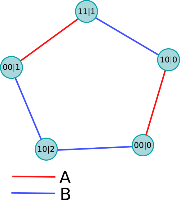
For example, in the case of the pentagon in the instrumental scenario we have two colors, and thus two graph $G_{A}$ and $G_{B}$, corresponding to variables $A$ and $B$ respectively, as shown in Fig. 6. Applying the technique described above to this scenario yields a quantum bound of $2.2071$, reproducing the known value for the quantum bound of the Bonet inequality given by $(3+\sqrt{2})/2$.

There are no quantum violation for instrumental scenarios with $l=2$ settings.

It is easy to see that no quantum violation is possible for instrumental scenario with $l=2$ possible settings for the instrumental variable $X$. This reduces to proving that there are no odd $n$-cycles nor $n$-anticycles as induced subgraphs in the corresponding exclusivity graph, with $n\geq 5$. To see this we can notice that any such graph is composed by two cliques (see for example Fig. 7), corresponding to the events with $x=0$ and $x=1$.

Figure 7: Exclusivity graph for the instrumental scenario $233$, showing the impossibility of having cycles with more than $5$ vertices. To simplify the figure cliques are represented by bold lines between vertices.

Any $n$-cycle with at least $5$ vertices must then have at least $3$ mutually connected vertices belonging to the same $x$, so they can never form a cycle-graph. Similarly we can show that there cannot be any induced odd anti-cycle with $5$ or more vertices.

There are no cycles $C_{n}$ with $n\geq 7$ in the $l22$ instrumental scenario.

In the following we prove that there cannot be a odd anti-cycle with more than $5$ vertices in the exclusivity graph associated to an instrumental scenario of the type $l22$.

Figure 8: Proof of the impossibility of having cycles with $7$ nodes or more in the $d22$ scenario.

Two different events $ab|x$ and $a^{\prime}b^{\prime}|x^{\prime}$, are exclusive if one of these two conditions is true:

1. $x=x^{\prime}$.

2. $a=a^{\prime}$ and $b\neq b^{\prime}$.

Suppose we have a cycle $C_{n}$ with $n\geq 7$, as in fig. 8, and consider that node $2$ in this graph corresponds to an event which we can arbitrarily identify as $00|0$. Among its neighbors $1$ and $3$, one will necessarily need to satisfy rule 2 (they cannot both satisfy rule 1 or the three nodes would be a clique. So without loss of generality we can assign the event $01|1$ to $3$. Since nodes $5,6,7$ must not satisfy rule 2 with both $2$ and $3$, then they must have $a=1$. Moreover $7$ and $5$ must have the same $b$, different from $6$. In the same way $1$ must not satisfy rule 2 with $6,5$ and $3$, so it needs to have $a=0$ and $b=1$. At this point, since we only have values $\{0,1\}$ for $a$, we cannot avoid node $4$ to be linked to one of the nodes $1,2,6,7$. Thus, the corresponding graph cannot be a cycle.

References

- [1] J. M. Mooij et al. Distinguishing cause from effect using observational data: methods and benchmarks., The Journal of Machine Learning Research 17, 1103 (2016).
- [2] J. Pearl, Causality: models, reasoning, and inference. Cambridge University Press, (2000).
- [3] J. Pearl, On the testability of causal models with latent and instrumental variables. Proceedings of the Eleventh conference on Uncertainty in artificial intelligence. Morgan Kaufmann Publishers Inc. (1995).
- [4] B. Bonet, Instrumentality tests revisited. Proceedings of the Seventeenth conference on Uncertainty in artificial intelligence. Morgan Kaufmann Publishers Inc. (2001).
- [5] J. M. Wooldridge, Introductory econometrics: A modern approach. Nelson Education, (2015).
- [6] R. R. Ramsahai, Causal bounds and observable constraints for non-deterministic models. Journal of Machine Learning Research 13, 829 (2012).
- [7] D. Kédagni, I. Mourifie, Generalized instrumental inequalities: Testing the IV independence assumption., available at SSRN (2017).
- [8] R. Chaves, G. Carvacho, I. Agresti, V. Di Giulio, L. Aolita, S. Giacomini, F. Sciarrino, Quantum violation of an instrumental test. Nature Physics 14.3 291 (2018).
- [9] T. Van Himbeeck, J. B. Brask, S. Pironio, R. Ramanathan, A. B. Sainz, E. Wolfe, Quantum violations in the Instrumental scenario and their relations to the Bell scenario. arXiv:1804.04119 (2018).
- [10] A. Cabello, S. Severini, A. Winter, Graph-theoretic approach to quantum correlations, Physical review letters, 112, 040401 (2014).
- [11] R. Rabelo, C. Duarte, A. J. López-Tarrida, M. T. Cunha, A. Cabello, Multigraph approach to quantum non-locality. Journal of Physics A: Mathematical and Theoretical, 47, 424021 (2014).
- [12] J. F. Clauser, M. A. Horne, A. Shimony, R. A. Holt, Proposed experiment to test local hidden-variable theories. Physical Review Letters 23, 880 (1969).
- [13] P. G. Wright, The tariff on animal and vegetable oils. The Macmillan Company, (1928).
- [14] C. W. J. Granger, Investigating causal relations by econometric models and cross-spectral methods. Econometrica, 424 (1969).
- [15] N. Cartwright, Causal Structures in Econometrics:On the Reliability of Economic Models. Recent Economic Thought Series 42, pp 63-89 (1995).
- [16] D. Janzing, et al. Quantifying causal influences. The Annals of Statistics 41, 2324 (2013).
- [17] J. S.Bell, On the Einstein Podolsky Rosen Paradox. Physics 1, 195 (1964).
- [18] K. Ried, M. Agnew, L. Vermeyden, D. Janzing, R. W. Spekkens, K. J. Resch, A quantum advantage for inferring causal structure. Nature Physics 11, 414 (2015).
- [19] F. Costa, S. Shrapnel, Quantum causal modelling. New Journal of Physics 18, 063032 (2016).
- [20] E. Wolfe, R. W. Spekkens, T. Fritz, The inflation technique for causal inference with latent variables. arXiv:1609.00672 (2016).
- [21] G. Carvacho, F. Andreoli, L. Santodonato, M. Bentivegna, R. Chaves, F. Sciarrino, Experimental violation of local causality in a quantum network. Nature communications, 8, 14775 (2017).
- [22] G. Carvacho, R. Chaves, F. Sciarrino, Perspectives on experimental quantum causality. EPL (Europhysics Letters), Volume 125, Number 3
- [23] A. Acín, T. Fritz, A. Leverrier, A. B. Sainz, A combinatorial approach to nonlocality and contextuality. Communications in Mathematical Physics 334, 533 (2015).
- [24] M. A. Nielsen, I. Chuang, Quantum computation and quantum information. (2002)
- [25] M. Navascués, Y. Guryanova, M. J. Hoban, A. Acín, Almost quantum correlations. Nature Communications 6, (2015).
- [26] M. Navascués, S. Pironio, A. Acín, A convergent hierarchy of semidefinite programs characterizing the set of quantum correlations. New Journal of Physics 10, 073013 (2008).
- [27] D. Knuth, The sandwich theorem. The Electronic Journal of Combinatorics 1, 1 (1994).
- [28] L. Lovász, An Algorithmic Theory of Numbers, Graphs, and Convexity. CBMS Regional Conference Series in Applied Mathematics (1986), §3.2.
- [29] J. Henson, R. Lal, M. F. Pusey, Theory-independent limits on correlations from generalized Bayesian networks. New Journal of Physics 16, 113043 (2014).
- [30] D. Collins, N. Gisin, N. Linden, S. Massar, S. Popescu, Bell inequalities for arbitrarily high-dimensional systems. Physical review letters 88, 040404 (2002).
- [31] M. Chudnovsky, N. Robertson, P. Seymour, R. Thomas, The strong perfect graph theorem. Annals of mathematics, 51-229 (2006).