Magnetisation dynamics of the compensated ferrimagnet Mn₂Ru_xGa

Abstract

Here we study both static and time-resolved dynamic magnetic properties of the compensated ferrimagnet Mn₂Ru_xGa from room temperature down to $10\text{\,}\mathrm{K}$, thus crossing the magnetic compensation temperature $T_{M}$. The behaviour is analysed with a model of a simple collinear ferrimagnet with uniaxial anisotropy and site-specific gyromagnetic ratios. We find a maximum zero-applied-field resonance frequency of $\sim$160\text{\,}\mathrm{GHz}$$ and a low intrinsic Gilbert damping $\alpha\sim 0.02$, making it a very attractive candidate for various spintronic applications.

I Introduction

Antiferromagnets (AFM) and compensated ferrimagnets (FiM) have attracted a lot of attention over the last decade due to their potential use in spin electronicsShick et al. (2010); Caretta et al. (2018). Due to their lack of a net magnetic moment, they are insensitive to external fields and create no demagnetising fields of their own. In addition, their spin dynamics reach much higher frequencies than those of their ferromagnetic (FM) counterparts due to the contribution of the exchange energy in the magnetic free energyGomonay and Loktev (2014).

Despite these clear advantages, AFMs are scarcely used apart from uni-directional exchange biasing relatively in spin electronic applications. This is because the lack of net moment also implies that there is no direct way to manipulate their magnetic state. Furthermore, detecting their magnetic state is also complicated and is usually possible only by neutron diffraction measurementsShull and Smart (1949), or through interaction with an adjacent FM layerJungwirth et al. (2016).

Compensated, metallic FiMs provide an interesting alternative as they combine the high-speed advantages of AFMs with those of FMs, namely, the ease to manipulate their magnetic state. Furthermore, it has been shown that such materials are good candidates for the emerging field of All-Optical Switching (AOS) in which the magnetic state is solely controlled by a fast laser pulse Stanciu et al. (2007); Mangin et al. (2014); Banerjee et al. (2019). A compensated, half-metallic ferrimagnet was first envisaged by van Leuken and de Groot (1995). In their model two magnetic ions in crystallographically different positions couple antiferromagnetically and perfectly compensate each-other, but only one of the two contributes to the states at the Fermi energy responsible for electronic transport. The first experimental realisation of this, Mn₂Ru_xGa (MRG), was provided by Kurt et al. (2014).

MRG crystallises in the $XA$ Heusler structure, space group $F\bar{4}3m$, with Mn on the $4a$ and $4c$ sitesBetto et al. (2015). Substrate-induced bi-axial strain imposes a slight tetragonal distortion, which leads to perpendicular magnetic anisotropy. Due to the different local environment of the two sublattices, the temperature dependence of their magnetic moments differ, and perfect compensation is therefore obtained at a specific temperature $T_{M}$ that depends on the Ru concentration $x$ and the degree of biaxial strain. It was previously shown that MRG exhibits properties usually associated with FMs: a large anomalous Hall angleThiyagarajah et al. (2015), that depends only on the magnetisation of the $4c$ magnetic sublatticeFowley et al. (2018); tunnel magnetoresistance (TMR) of $40\text{\,}\mathrm{\char 37\relax}$, a signature of its high spin polarisationŽic et al. (2016), was observed in magnetic tunnel junctions (MTJs) based on MRGBorisov et al. (2016); and a clear magneto-optical Kerr effect and domain structure, even in the absence of a net momentFleischer et al. (2018); Siewierska et al. (2019). Strong exchange bias of a CoFeB layer by exchange coupling with MRG through a Hf spacer layerBorisov et al. (2017), as well as single-layer spin-orbit torqueTroncoso et al. (2019); Lenne et al. (2019) showed that MRG combined the qualities of FMs and AFMs in spin electronic devices.

The spin dynamics in materials where two distinct sublattices are subject to differing internal fields (exchange, anisotropy, …) is much richer than that of a simple FM, as previously demonstrated by the obersvation of single-pulse all-optical switching in amorphous GdFeCoStanciu et al. (2006); Radu et al. (2011) and very recently in MRGBanerjee et al. (2019). Given that the magnetisation of MRG is small, escpecially close to the compensation point, and the related frequency is high, normal ferromagnetic resonance (FMR) spectroscopy is unsuited to study their properties. Therefore, we used the all-optical pump-probe technique to characterize the resonance frequencies at different temperatures in vicinity of the magnetic compensation point. This, together with the simulation of FMR, make it possible to determine the effective g-factors, the anisotropy constants and their evolution across the compensation point. We found, in particular, that our ferrimagnetic half-metallic Heusler alloy has resonance frequency up to 160 GHz at zero-field and a relatively low Gilbert damping.

II Experimental details

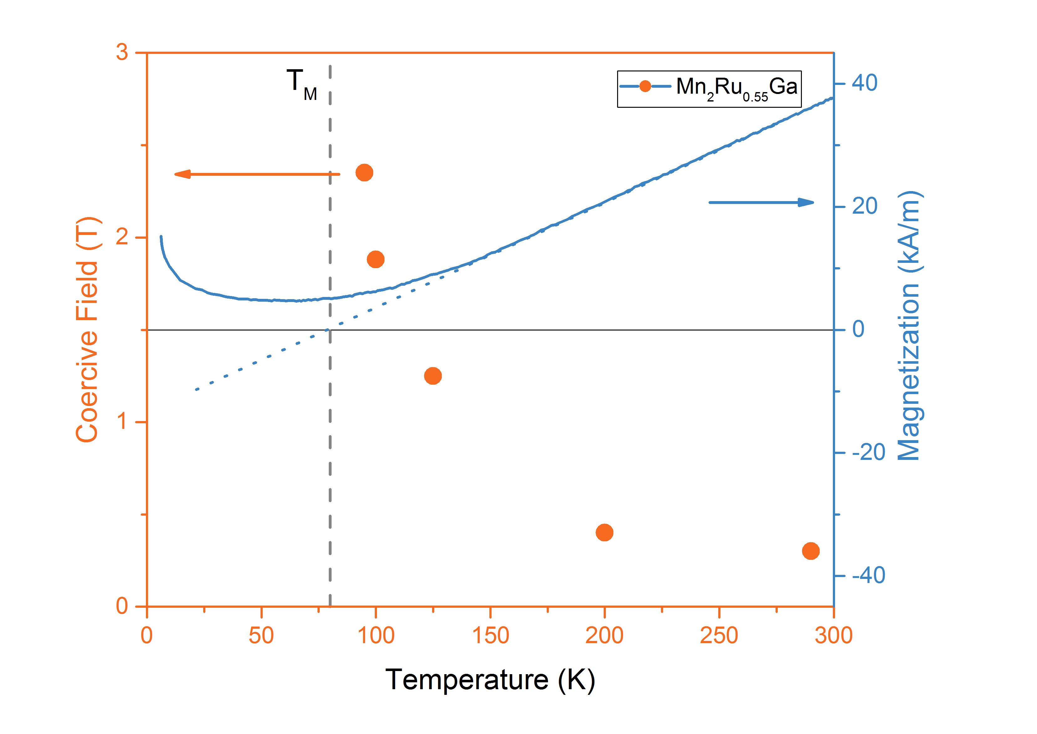
Figure 1: Net moment measured by magnetometry and coercive field measured by static Faraday effect. The upturn of the net moment below $T\sim$50\text{\,}\mathrm{K}$$ is due to paramagnetic impurities in the MgO substrate. $T_{M}$ is indicated by the vertical dotted line. As expected the maximum available applied field $\mu_{0}H=$7\text{\,}\mathrm{T}$$ is insufficient to switch the magnetisation close to $T_{M}$.

Thin film samples of MRG were grown in a ‘Shamrock’ sputter deposition cluster with a base pressure of $2\text{\times}{10}^{-8}\text{\,}\mathrm{T}\mathrm{o}\mathrm{r}\mathrm{r}$ on MgO (001) substrates. Further information on sample deposition can be found elsewhereBetto et al. (2016). The substrates were kept at $250\text{\,}\mathrm{\SIUnitSymbolCelsius}$, and a protective $\sim$3\text{\,}\mathrm{nm}$$ layer of aluminium oxide was added at room temperature. Here we focus on a $53\text{\,}\mathrm{nm}$ thick sample with $x=0.55$, leading to $T_{M}\approx$80\text{\,}\mathrm{K}$$ as determined by SQUID magnetometry using a Quantum Design $5\text{\,}\mathrm{T}$ MPMS system (see Figure 1). We are able to study the magneto-optical properties both above and below $T_{M}$.

The magnetisation dynamics was investigated using an all-optical two-colour pump-probe scheme in a Faraday geometry inside a $\mu_{0}H_{\text{max}}=$7\text{\,}\mathrm{T}$$ superconducting coil-cryostat assembly. Both pump and probe were produced by a Ti:sapphire femtosecond pulsed laser with a central wavelength of $800\text{\,}\mathrm{nm}$, a pulse width of $40\text{\,}\mathrm{fs}$ and a repetition rate of $1\text{\,}\mathrm{kHz}$. After splitting the beam in two, the high-intensity one was doubled in frequency by a BBO crystal (giving $\lambda=$400\text{\,}\mathrm{nm}$$) and then used as the pump while the lower intensity $800\text{\,}\mathrm{nm}$ beam acted as the probe pulse. The time delay between the two was adjusted by a mechanical delay stage. The pump was then modulated by a synchronised mechanical chopper at $500\text{\,}\mathrm{Hz}$ to improve the signal to noise ratio by lock-in detection. Both pump and probe beams were linearly polarized, and with spot sizes on the sample of $150\text{\,}\mathrm{\SIUnitSymbolMicro m}70\text{\,}\mathrm{\SIUnitSymbolMicro m}$, respectively. The pump pulse hit the sample at an incidence angle of $\approx$10\text{\,}\mathrm{\SIUnitSymbolDegree}$$. After interaction with the sample, we split the probe beam in two orthogonally polarized parts using a Wollaston prism and detect the changes in transmission and rotation by calculating the sum and the difference in intensity of the two signals.

The external field was applied at $75\text{\,}\mathrm{\SIUnitSymbolDegree}$ to the easy axis of magnetization thus tilting the magnetisation away from the axis. Upon interaction with the pump beam the magnetisation is momentarily drastically changedKoopmans et al. (2005) and we monitor its return to the initial configuration via remagnetisation and then precession through the time dependent Faraday effect on the probe pulse.

The static magneto-optical properties were examined in the same cryostat/magnet assembly.

III Results & discussion

III.1 Static magnetic properties

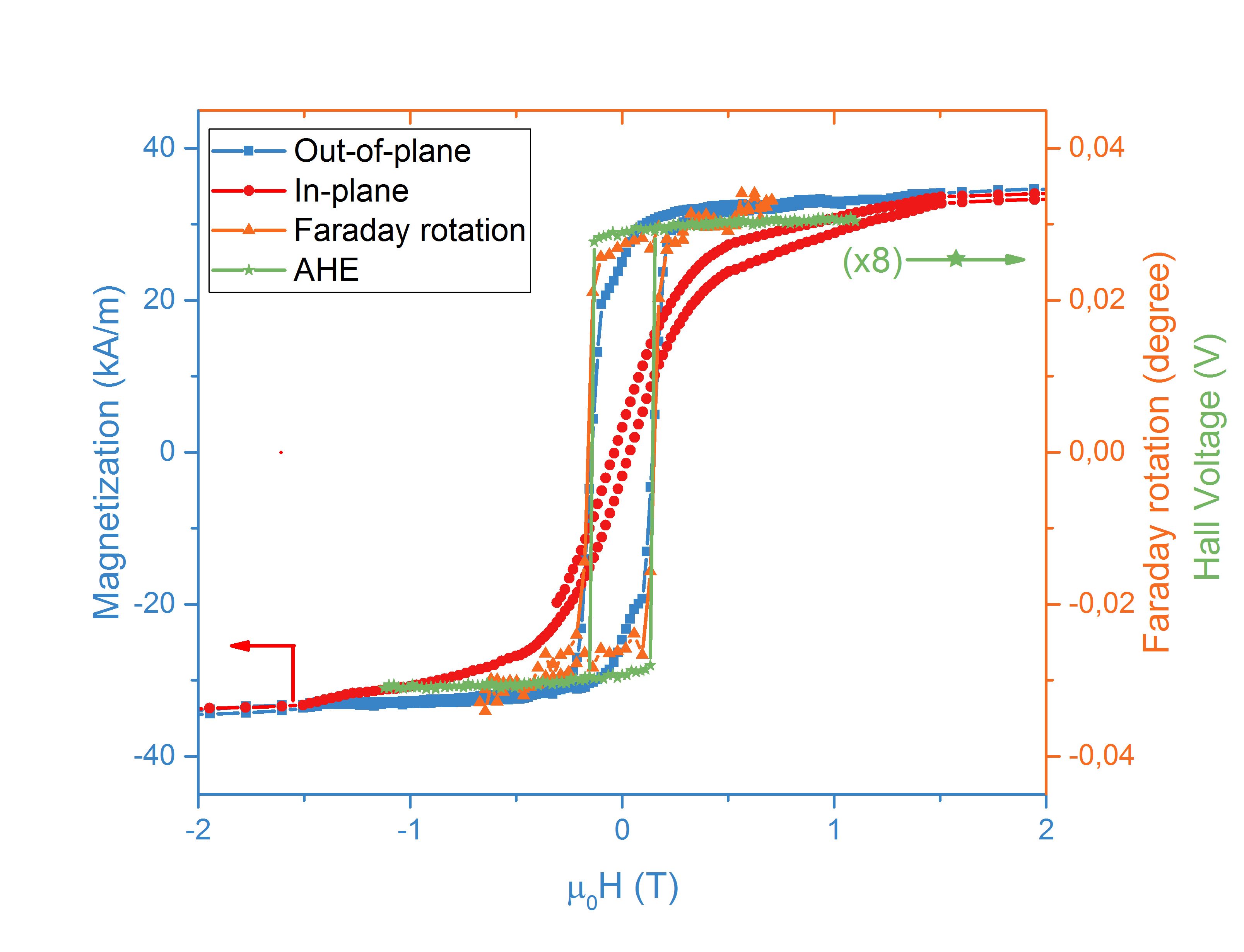
Figure 2: Comparison of hysteresis loops obtained by Faraday, AHE, and magnetometry recorded at room temperature. The two former were recorded with the applied field perpendicular to the sample surface, while for the latter we show results for both field applied parallel and perpendicular to the sample.

We first focus on the static magnetic properties as observed by the Faraday effect, and compare them to what is inferred from magnetometry and the anomalous Hall effect. In Figure 2 we present magnetic hysteresis loops as recorded using the three techniques. Due to the half metallic nature of the sample, the magnetotransport properties depend only on the $4c$ sublattice. As the main contribution to the MRG dielectric tensor in the visible and near infrared arises from the Drude tailFleischer et al. (2018), both AHE and Faraday effect probe essentially the same properties (mainly the spin polarised conduction band of MRG), hence we observe overlapping loops for the two techniques. Magnetometry, on the other hand, measures the net moment, or to be precise the small difference between two large sublattice moments. The $4a$ sublattice, which is insignificant for AHE and Faraday here contributes on equal footing. Figure 2 shows a clear difference in shape between the magnetometry loop and the AHE or Faraday loops. We highlight here that the apparent ‘soft’ contribution that shows switching close to zero applied field, is not a secondary magnetic phase, but a signature of the small differences in the field-behaviour of the two sublattices. We also note that this behaviour is a result of the non-collinear magnetic order of MRG. A complete analysis of the dynamic properties therefore requires knowledge of the anisotropy constants on both sublattices as well as the (at least) three intra and inter sublattice exchange constants. Such an analysis is beyond the scope of this article, and we limit our analysis to the simplest model of a single, effective uniaxial anisotropy constant $K_{u}$ in the exchange approximation of the ferrimagnet.

III.2 Dynamic properties

We now turn to the time-resolved Faraday effect and spin dynamics. Time-resolved Faraday effect data were recorded at five different temperatures $10\text{\,}\mathrm{K}50\text{\,}\mathrm{K}100\text{\,}\mathrm{K}200\text{\,}\mathrm{K}290\text{\,}\mathrm{K}$, with applied fields ranging from $1\text{\,}\mathrm{T}7\text{\,}\mathrm{T}$.

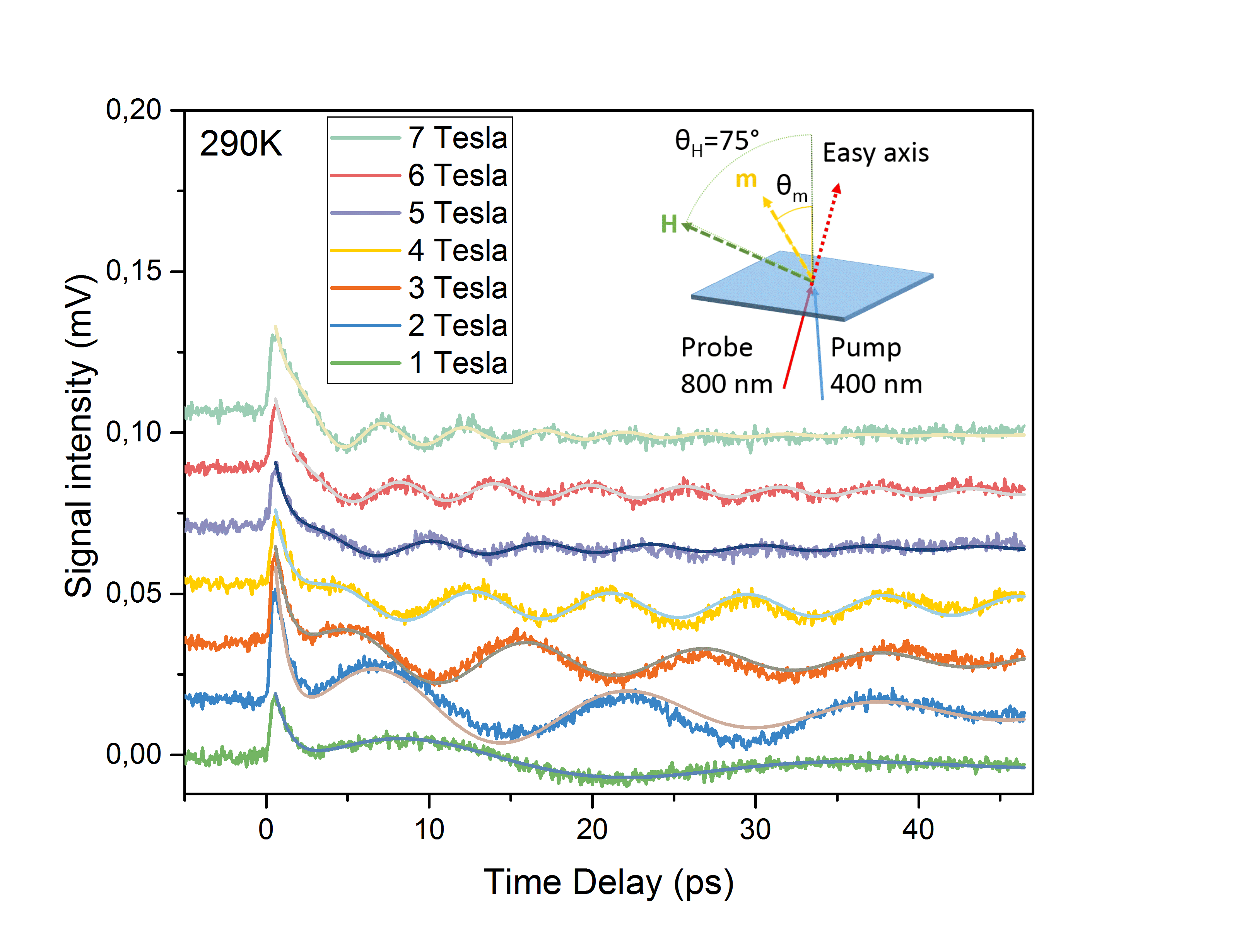
Figure 3: Time resolved Faraday effect recorded at $T=$290\text{\,}\mathrm{K}$$ in applied fields ranging from $1\text{\,}\mathrm{T}7\text{\,}\mathrm{T}$. After the initial demagnetisation seen as a sharp increase in the signal at $t\sim$0\text{\,}\mathrm{ps}$$, magnetisation is recovered and followed by precession around the effective field until fully damped. The lines are fits to the data. The inset shows the experimental geometry further detailed in the main text.

Figure 3 shows the field-dependence of the Faraday effect as a function of the delay between the pump and the probe pulses, recorded at $T=$290\text{\,}\mathrm{K}$$. Negative delay indicates the probe is hitting the sample before the pump. After the initial demagnetisation, the magnetisation recovers and starts precessing around the effective field which is determined by the anisotropy and the applied field. The solid lines in Figure 3 are fits to the data to extract the period and the damping of the precession in each case. The fitting model was an exponentially damped sinusoid with a phase offset. We note that the apparent evolution of the amplitude and phase with changing applied magnetic field is due to the quasi-resonance of the spectrum of the precessional motion with the low-frequency components of the convolution between the envelope of the probe pulse and the physical relaxation of the system. The latter include both electron-electron and electron-lattice effects. A rudimentary model based on a classical oscillator successfully reproduces the main features of the amplitude and phase observed.

In two-sublattice FiMs, the gyromagnetic ratios of the two sublattices are not necessarily the same. This is particularly obvious in rare-earth/transition metal alloys, and is also the case for MRG  despite the two sublattices being chemically similar; they are both Mn. Due to the different local environment however, the degree of charge transfer for the two differs. This leads to two characteristic temperatures, a first $T_{M}$ where the magnetic moments compensate, and a second $T_{A}$ where the angular momenta compensate. It can be shown that for the ferromagnetic mode, the effective gyromagnetic ratio $\gamma_{\text{eff}}$ can then be writtenWangsness (153)

$$\gamma_{\text{eff}}=\frac{M_{4c}(T)-M_{4a}(T)}{M_{4c}(T)/\gamma_{4c}-M_{4a}(T)/\gamma_{4a}}$$ (1)

subscript $i=4a,4c$ denotes sublattice $i$, $M_{i}(T)$ the temperature-dependent magnetisation, and $\gamma_{i}$ the sublattice-specific gyromagnetic ratio. $\gamma_{\text{eff}}$ is related to the effective $g$-factor

$$g_{\text{eff}}=\gamma_{\text{eff}}\frac{h}{\mu_{B}}$$ (2)

where $h$ is the Planck constant and $\mu_{B}$ the Bohr magneton.

The frequency of the precession is determined by the effective field, which can be inferred from the derivative of the magnetic free energy density with respect to $\mathbf{M}$. For an external field applied at a given fixed angle with respect to the easy axis this leads to the Smit-Beljers formulaSmit and Beljers (1955)

$$\omega_{FMR}=\gamma_{\text{eff}}\sqrt{\frac{1}{M_{s}^{2}sin^{2}\phi}\left[\frac{\delta^{2}E}{\delta\theta^{2}}\frac{\delta^{2}E}{\delta\phi^{2}}-\left(\frac{\delta^{2}E}{\delta\theta\delta\phi}\right)^{2}\right]}$$ (3)

where $\theta$ and $\phi$ are the polar and azimuthal angles of the magnetisation vector, and $E$ the magnetic free energy density

$$E=-\mu_{0}\mathbf{H}\cdot\mathbf{M}+K_{u}\sin^{2}{\theta}+\mu_{0}M_{s}^{2}\cos^{2}{\theta}/2$$ (4)

where the terms correspond to the Zeeman, anisotropy and demagnetising energies, respectively, and $M_{s}$ is the net saturation magnetisation. It should be mentioned that the magnetic anisotropy constant $K_{u}$ is related to $M$, which is being considered constant in magnitude, via $K_{u}=\beta\mu_{0}M_{s}^{2}/2$, $\beta$ a dimensionless parameter.

Based on Eqs. (1) through (4) we fit our entire data set with $\gamma_{\text{eff}}$ and $K_{u}$ as the only free parameters. The experimental data and the associated fits are shown as points and solid lines in Figure 4. At all temperatures our simple model with one effective gyromagnetic ratio $\gamma_{\text{eff}}$ and a single uniaxial anisotropy parameter $K_{u}$ reproduces the experimental data reasonably well. The model systematically underestimates the resonance frequency for intermediate fields, with the point of maximum disagreement increasing with decreasing temperature. We speculate this is due to the use of a simple uniaxial anisotropy in the free energy (see Eq. 4), while the real situation is more likely to be better represented as a sperimagnet. In particular, the non-collinear nature of MRG that leads to a deviation from $180\text{\,}\mathrm{\SIUnitSymbolDegree}$ of the angle between the two sublattice magnetisations, depending on the applied field and temperature.

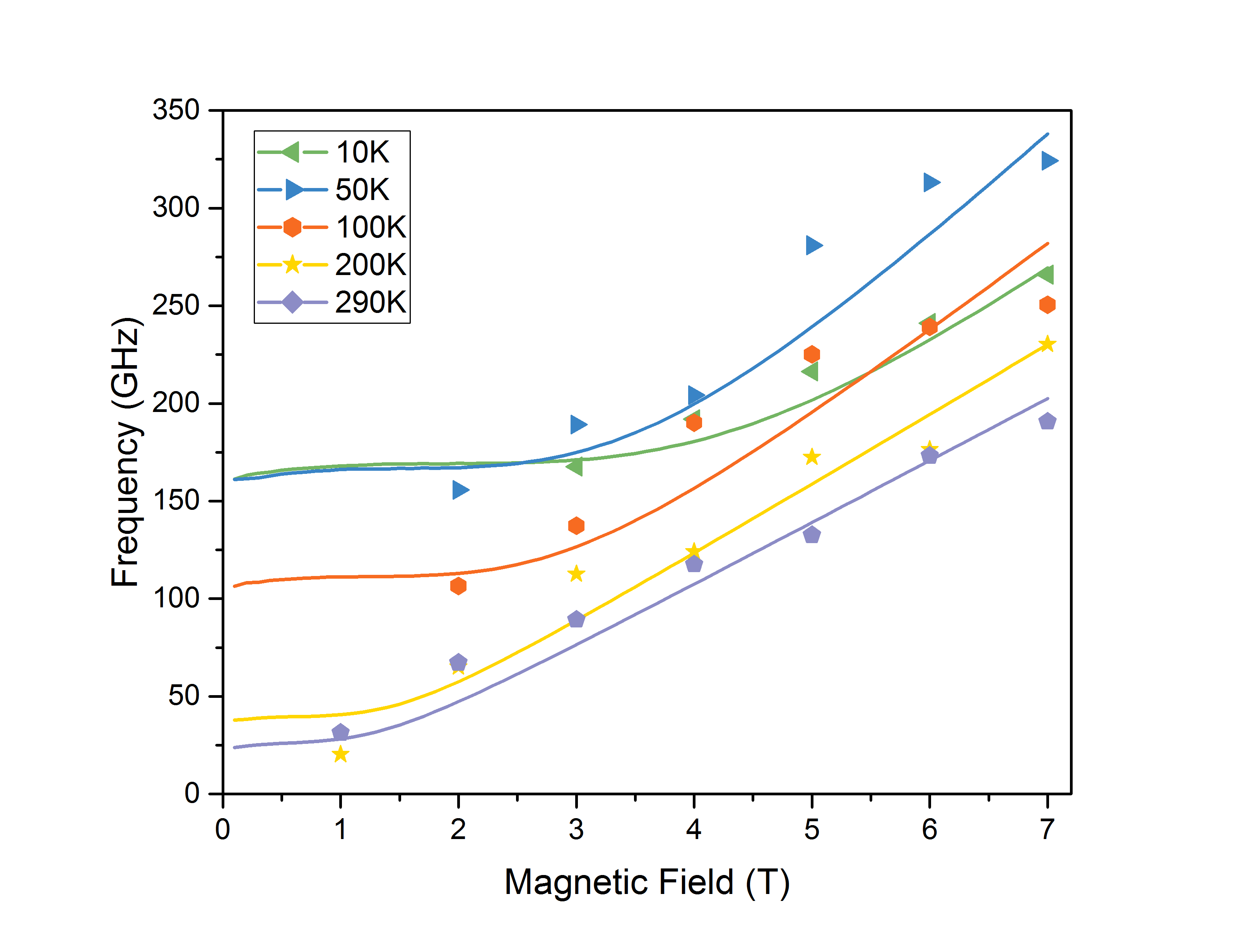
Figure 4: Observed precession frequency as a function of the applied field for various temperatures. The solid lines are fits to the data as described in the main text.

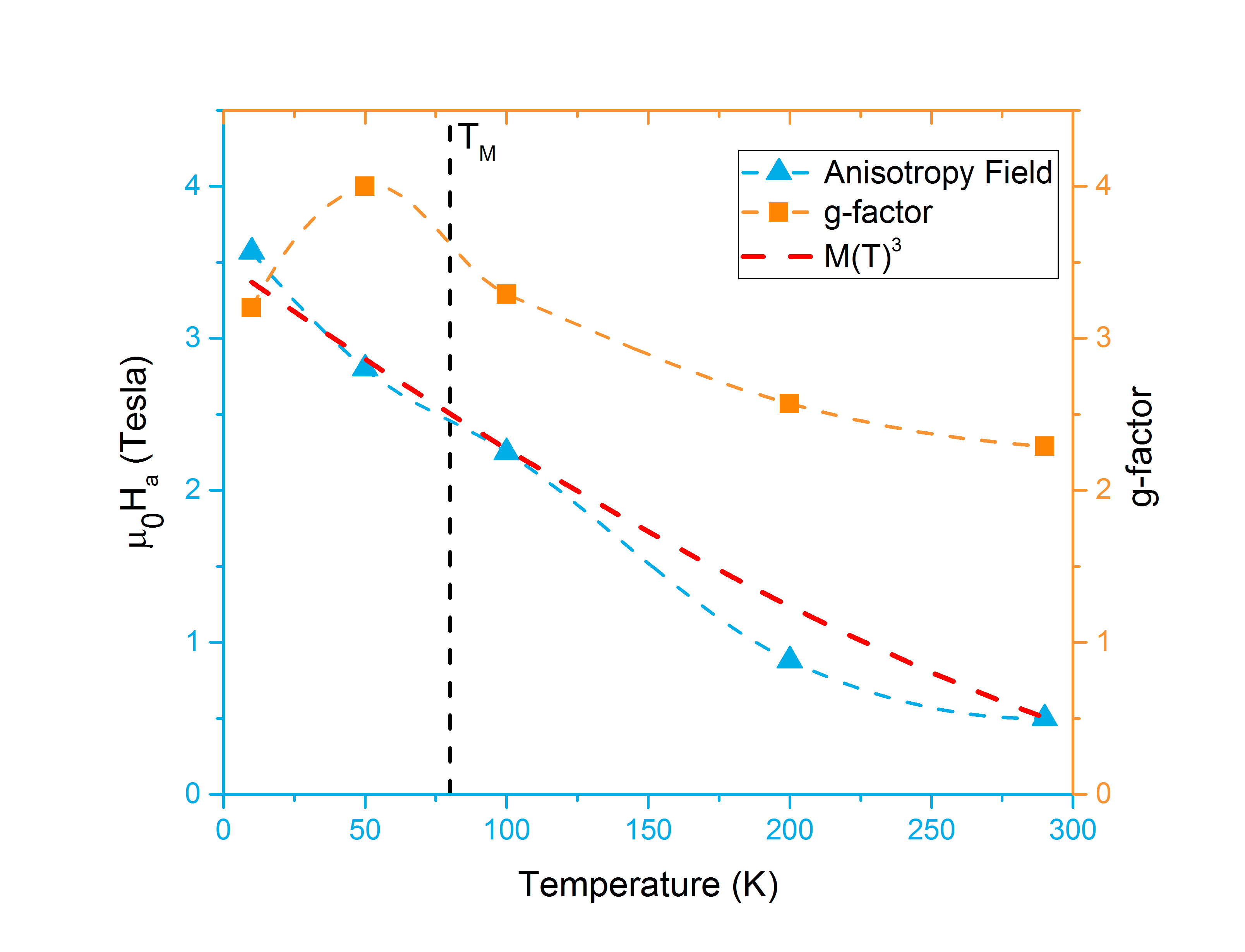
Figure 5: Effective $g$-factor, $g_{\text{eff}}$, and the anisotropy field as determined by time-resolved Faraday effect. $g_{\text{eff}}$, orange squares, increases from near the free electron value of 2 to 4 just below $T_{M}$, while the anisotropy field, blue triangles, increases near-linearly with decreasing temperature. A $M^{3}$ fit, red dashes line, of the anisotropy behaviour shows the almost-metallic origin of it, indicating the dominant character of the 4c sublattice.

From the fits in Figure 4 we infer the values of $g_{\text{eff}}$ and the anisotropy field $\mu_{0}H_{a}={}^{2K_{u}}\!/\!_{M_{s}}$. The result is shown in Figure 5. The anisotropy field is monotonically increasing with decreasing temperature as the magnetisation of the $4c$ sublattice increases in the same temperature range. We highlight here the advantage of determining this field through time-resolved magneto-optics as opposed to static magnetometry and optics. Indeed the anisotropy field as seen by static methods is sensitive to the combination of anisotropy and the net magnetic moment, as illustrated in Figure 1, where the coercive field diverges as $T\rightarrow T_{M}$. In statics one would expect a divergence of the anisotropy field at the same temperature. The time-resolved methods however distinguish between the net and the sublattice moments, hence better reflecting the evolution of the intrinsic material properties of the ferrimagnet.

The temperature dependence of the anisotropy constants was a matter for discussion for many yearsCallen and Callen (1966); Vonsovskii (1974). Written in spherical harmonics the $3d$ anisotropy can be expressed as, $k_{2}Y_{2}^{0}(\theta)+k_{4}Y_{4}^{0}(\theta)$  Farle (1998) where $k_{2}\propto M(T)^{3}$ and $k_{4}\propto M(T)^{10}$. The experimental measured anisotropy is then, $K_{2}(T)=ak_{2}(T)+bk_{4}(T)$, with $a$ and $b$ the contributions of the respective spherical harmonics.

Figure 5 shows that a reasonable fit of our data is obtained with $M(T)^{3}$ which means, first, that the contribution of the $4^{th}$ order harmonic can be neglected, and second, that the contribution of the $T_{M}$ and $2^{nd}$ sublattice is negligible, indicating the dominant character of the 4c sublattice.

In addition, we should note here that the high frequency exchange mode was never observed on our experiments. While far from $T_{M}$ its frequency might be too high to be observable, in the vicinity of $T_{M}$, in contrast, its frequency is expected to be in the detection range. Moreover, given the different electronic structure of the two sublattices, it is expected that the laser pulse should selectively excite the sublattice 4c, and therefore lead to the effective excitation of the exchange mode. We argue that it is the non-collinearity of the sublattices (see section III A) that smears out the coherent precession at high frequencies.

The effective gyromagnetic ratio, $g_{\text{eff}}$, shows a non-monotonic behaviour. It increases with decreasing $T$ towards $T_{M}$, reaching a maximum at about $50\text{\,}\mathrm{K}$ before decreasing again at $T=$10\text{\,}\mathrm{K}$$. We alluded above to the difference between the magnetic and the angular momenta compensation temperatures. We expect that $g_{\text{eff}}$ reaches a maximum when $T=T_{A}$Gurevich and Melkov (1996), here between the measurement at $T=$50\text{\,}\mathrm{K}$$ and the magnetic compensation temperature $T_{M}\approx$80\text{\,}\mathrm{K}$$.

From XMCD dataBetto et al. (2015), we could estimate spin and orbital moment components of the magnetic moments of the two sublattices, what allowed us to derive the effective g-factors for the sublattices as $g_{4a}=2.05$ and $g_{4c}=2.00$. In this case we expect the angular momentum compensation temperature $T_{A}$ to be below $T_{M}$, opposite to what is observed for GdFeCoStanciu et al. (2006). Given this small difference however, $T_{A}$ and $T_{M}$ are expected to be rather close to each other, consistent with the limited increase of $g_{\text{eff}}$ across the compensation points.

We turn finally to the damping of the precessional motion of $\mathbf{M}$ around the effective field $\mu_{0}\mathbf{H_{\text{eff}}}$. Damping is usually described via the dimensionless parameter $\alpha$ in the Landau-Lifshiz-Gilbert equation, and it is a measure of the dissipation of magnetic energy in the system. In this model, $\alpha$ is a scalar constant and the observed broadening in the time domain is therefore a linear function of the frequency of precessionMalinowski et al. (2009); Liu et al. (2010); Schellekens et al. (2013). We infer $\alpha^{\prime}$, the total damping, from our fits of the time-resolved Faraday effect as $\alpha^{\prime}=\left(\tau_{d}\right)^{-1}$, where $\tau_{d}$ is the decay time of the fits. We then, for each temperature, plot $\alpha^{\prime}$ as a function of the observed frequency and regress the data using a straight line fit. The intrinsic $\alpha$ is the slope of this line, while the intercept represents the anisotropic broadening.

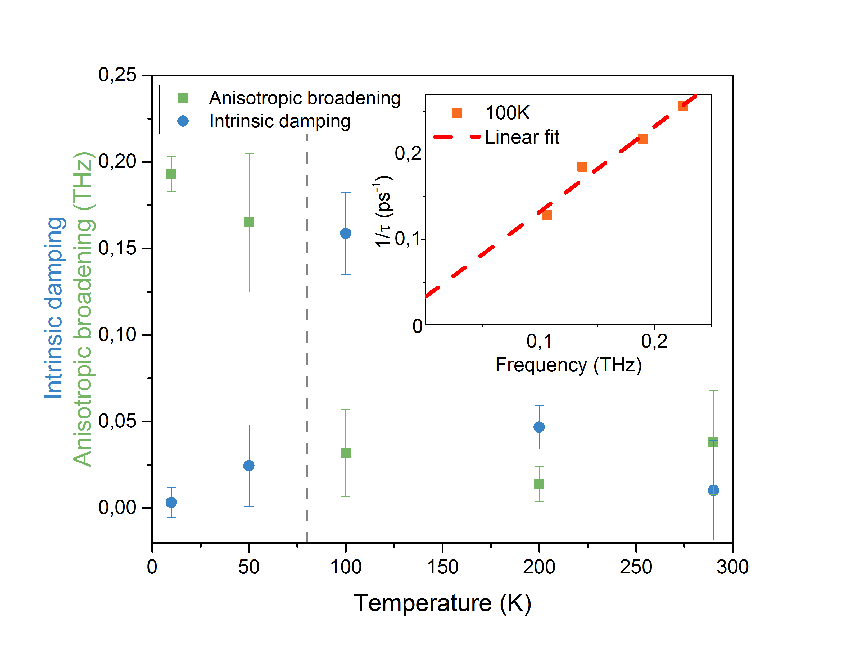
Figure 6: Intrinsic and anisotropic broadening in $MRG$ across the $T_{M}$. The inset shows the evaluation process of the two damping parameters. A linear fit is used to evaluate intercept (anisotropic broadening) and slope (intrinsic damping) of the frequencies versus the inverse of the decay time. The data point are obtained from the fit of time-resolved Faraday effect measurements (an example is shown in Fig.4).

Figure 6 shows the intrinsic damping $\alpha$ and the anisotropic broadening as a function of temperature. Anisotropic broadening is usually attributed to a variation of the anisotropy field in the region probed by the probe pulseWalowski et al. (2008). For MRG this is due to slight lateral variations in the Ru content $x$ in the thin film sample. Such a variation leads to a variation in effective $T_{M}$ and $T_{A}$ and can therefore have a large influence on the broadening as a function of temperature. Despite this, the anisotropic broadening is reasonably low in the entire temperature range above $T_{M}$, and a more likely explanation for its rapid increase below $T_{M}$ is that the applied magnetic field is insufficient to completely remagnetize the sample between two pump pulses. As observed in Fig.5, the anisotropy field reaches almost $4\text{\,}\mathrm{T}$ at low temperature, comparable to our maximum applied field of $7\text{\,}\mathrm{T}$. The intrinsic damping $\alpha$ is less than 0.02 far from $T_{M}$, but increases sharply at $T=$100\text{\,}\mathrm{K}$$. We tentatively attribute this to an increasing portion of the available power being transferred into the high-energy exchange mode, although we underline that we have not seen any direct evidence of such a mode in any of the experimental data.

IV Conclusion

We have shown that the time-resolved Faraday effect is a powerful tool to determine the spin dynamic properties in compensated, metallic ferrimagnets. The high spin polarisation of MRG enables meaningful Faraday data to be recorded even near $T_{M}$ where the net magnetisation is vanishingly small, and the dependence of the dynamics on the sublattice as opposed to the net magnetic properties provides a more physical understanding of the material. Furthermore, we find that the ferromagnetic-like mode of MRG reaches resonance frequencies as high as $160\text{\,}\mathrm{GHz}$ in zero applied field, together with a small intrinsic damping. This value is remarkable if compared to well-known materials such as GdFeCo which, at zero field, resonates at tens of GHzStanciu et al. (2006) or $[\text{Co/Pt}]_{n}$ multilayers at $80\text{\,}\mathrm{GHz}$Barman et al. (2007) but with higher damping. We should however stress that, in the presence of strong anisotropy fields, higher frequencies can be reached. Example of that can be found for ferromagnetic Fe/Pt with $\approx$280\text{\,}\mathrm{GHz}$$ ($H_{a}=10T$)Becker et al. (2014), and for Heusler-like ferrimagnet (Mn₃Ge and Mn₃Ga) with $\approx$500\text{\,}\mathrm{GHz}$$ ($H_{a}=20T$)Mizukami et al. (2016); Awari et al. (2016). Nevertheless, the examples cited above show a considerably higher intrinsic damping compared to MRG. In addition, it was recently shown that MRG exhibits unusually strong intrinsic spin-orbit torqueLenne et al. (2019). Thus, taking into account the material parameters we have determined here, it seems likely it will be possible to convert a DC driven current into a sustained ferromagnetic resonance at $f=$160\text{\,}\mathrm{G}\mathrm{Hz}$$, at least. These characteristics make MRG, as well as any future compensated half-metallic ferrimagnet, particularly promising materials for both spintronics and all-optical switching.