Extracting Conceptual Knowledge from Natural Language Text Using Maximum Likelihood Principle

Abstract

Domain-specific knowledge graphs constructed from natural language text are ubiquitous in today’s world. In many such scenarios the base text, from which the knowledge graph is constructed, concerns itself with practical, on-hand, actual or ground-reality information about the domain. Product documentation in software engineering domain are one example of such base texts. Other examples include blogs and texts related to digital artifacts, reports on emerging markets and business models, patient medical records, etc.

Though the above sources contain a wealth of knowledge about their respective domains, the conceptual knowledge on which they are based is often missing or unclear. Access to this conceptual knowledge can enormously increase the utility of available data and assist in several tasks such as knowledge graph completion, grounding, querying, etc. Additionally, this conceptual knowledge can also be used to find common semantics across different knowledge graphs.

Our contributions in this paper are twofold. First, we propose a novel Markovian stochastic model for document generation from conceptual knowledge. This model is based on the assumption that a writer generates successive sentences of a text only based on her current context as well as the domain-specific conceptual knowledge in her mind. The uniqueness of our approach lies in the fact that the conceptual knowledge in the writer’s mind forms a component of the parameter set $\lambda$ of our stochastic model.

Secondly, we solve the inverse problem of learning the best conceptual knowledge from a given document ${\bf O}$, by finding model parameters $\lambda^{*}$ which maximize the likelihood of generating document ${\bf O}$ over all possible parameter values. This likelihood maximization is done using an application of Baum-Welch algorithm, which is a known special case of Expectation-Maximization (EM) algorithm.

We run our conceptualization algorithm on several well-known natural language sources and obtain very encouraging results. The results of our extensive experiments concur with the hypothesis that the information contained in these sources has a well-defined and rigorous underlying conceptual structure, which can be discovered using our method.

1 Introduction

Knowledge needs to be sieved from natural language text: In today’s world, a simple search query on World Wide Web (WWW) specifically, on search engine such as Google, provides an enormous number of documents written in natural language. The search query and the resultant natural language documents can pertain to any particular domain of human knowledge. These natural language texts have a huge amount of multi-layered knowledge which must be made available in a machine understandable format to expert and intelligent automated decision-making systems. Whereas knowledge graphs have established themselves as the model of choice [1] for storing and operating on this information, they suffer from data overload [2] during querying due to the sheer volume of information involved [3, 4, 5, 6].

As a relevant example, the knowledge domain can be “software engineering” and the natural language texts may be “online documentations, discussion forums, bug reports, etc. for different software products”. Efficient mining of the wealth of experiential information contained in these online sources would allow one to automate in large part the different facets of software engineering and design processes.

Human domain experts seem to solve data overload problem using conceptualization. : Domain experts seem to routinely use human reasoning processes to acquire, build and update a high-level “conceptual” view of any particular knowledge domain by studying relevant documents most of which are rich in natural language text. This constant process of “conceptualization” allows domain experts to tackle the problem of information overload and to gain an in-depth knowledge of the domain over a period of several years. One can further postulate that this learnt conceptual view offers a guiding framework for the domain expert to provide specific and relevant answers to subject queries with minimal response time.

Conceptualization is highly useful because unlike the low-level and extensive entity-relation based viewpoint provided by a detailed knowledge graph, the expert’s conceptual view of data is several orders more concise and consists of very few concept classes along with specific relations between these concept classes. Moreover, it seems that this high-level conceptual view is overlayed over the low-level entity-relation based view in the expert’s mind i.e., for most entities in the domain of discourse, the expert is able to mark them as “instances” of one or more concept classes. This “overlaying” has the beneficial effect of summarization of the knowledge graph - the expert now needs to remember only a small number of outlier relations (or, exceptions) as she can now “approximately” derive most relations between entity pairs from corresponding relations between concept pairs to which these entities belong.

Motivation: Motivated by the importance of conceptualization in creation of robust human expertise in a given domain, this paper is an effort at designing reliable automated methods for arriving at high-level conceptual frameworks of a given domain using widely available natural language documents.

Such machine-generated high-level conceptual frameworks will have several applications for automated task engines including:

1. Knowledge graph identification[3] by removing unnecessary or wrong relationships and entities.

2. Uncovering underlying terminologies of a specific domain while hiding the minute details which can be queried further if required.

3. Handling information overload in gracious manner.

4. Forming a short, concept-based summary of domain knowledge and therefore reducing the memory needed for remembering the knowledge graph.

Contribution: The contributions of this paper are twofold:

1. Our first contribution is a new stochastic model for document generation from conceptual knowledge (see Section 2). Our model tries to emulate the mental processes of an expert writing a domain-specific document.

   Our model is based on the assumption that the expert generates a given document in a top-down manner by proceeding from conceptual knowledge to specific entity-level relations. We break this process down into three steps: (i) changing the current context, (ii) generating a valid concept pair relation based on the current context, and (iii) “instantiating” this concept pair relation to an entity-level relationship. Thus, our model has a large parameter set $\lambda$ which includes:

   • stationary and transition probabilities of a Markovian process for keeping track of current context,

   • output probabilities of generating a particular concept pair based on current context, and

   • parameters fully encoding the conceptual knowledge of the expert along with the membership probabilities of different entities in various concepts.

2. Our second contribution is an algorithm to learn the “most likely” conceptualization $C^{*}$ of domain knowledge given an input collection of domain-specific documents. In our framework, a conceptualization $C$ is considered more likely if a writer with conceptualization $C$ in her mind is more likely to generate the given document set as per our stochastic model. The problem of finding the most likely conceptualization is then solved by us by applying Baum-Welch algorithm [7].

   Rather surprisingly, as shown by our experimental results, even with a purely stochastic model we are able to derive high quality conceptualizations from natural language texts.

Figure 1 depicts the bird’s eye view of our contribution.

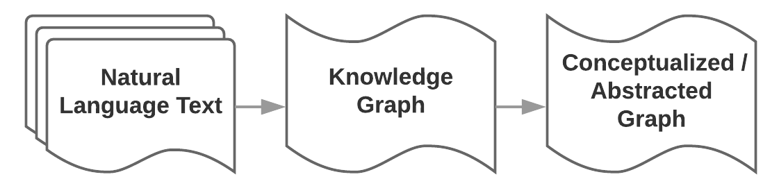
Figure 1: Our Contribution- Bird’s-eye view

Before going ahead with the details, we would like to list the salient features of our method:

Salient features and novelties of our method:

1. Our method optimizes over all possible conceptualizations in a global manner i.e., both concepts and their inter-relations form unknown parameters of our model. This is different from current approaches of having separate local methods for finding the concept classes and their inter-relations.

2. The identified concept classes are extracted from the underlying data itself and do not use any external knowledge graph or controlled vocabulary. Thus our method is not domain-specific and can be applied to document collections in any domain.

3. No restriction (for example, tree-like, is-a, etc.) is placed on the structure of the conceptualized knowledge graph. In fact, our algorithm learns the structure based on the particular input data.

4. Our model treats both taxonomic and non-taxonomic relations in a uniform manner.

5. Our method even allows entities which are not syntactically or lexically close to belong to the same concept class.

6. Our model is generic and allows the same entity to belong to more than one concept as is the case in the real world.

7. The ratio of original graph to conceptual graph is variable and thus the coarseness of the desired conceptualization can be changed by adjusting relevant parameters.

8. Very large concept classes are in general discouraged and entities are usually well-distributed across concept classes.

In our method, the abstracted knowledge graph construction from text occurs as a result of applying Baum-Welch on a single, constrained (but complex) HMM $\mathcal{H}$. This widely extends the usage of Hidden Markov Models and is a novel application of stochastic methods in this domain.

The paper is presented as follows. Section 2 discusses the proposed model to generate documents. In Section 3, we describe our algorithm to find the most likely model parameters given a base text. We discuss experimental setup and performance evaluation of our algorithm in Section 4. Section 5 discusses literature relevant to our work. Finally, in Section 6, we summarize our contributions and outline future work.

2 Our document generation model

We now describe our stochastic model for document generation by a domain expert.

In our model, we assume that a domain expert writes a document, one sentence at a time, from start to end. Further, we make the assumption that each sentence written by the expert is generated stochastically and depends on two factors: (i) the current context within the document, and (ii) the expert’s domain-specific conceptual knowledge.

We now describe the parameters of our document generation model. The reader is referred to Table I for a summary. In the table, the parameters are partitioned into two sets: first set of parameters relate to current context (see Section 2.1), whereas the second set of parameters model expert’s conceptual knowledge (see Section 2.2).

Parameters		Constraints	Interpretation
Context	Conceptual Knowledge
	$k$		Number of concepts in abstract/conceptual graph
$b$			Number of states in discrete Markov process $\mathcal{M}$
$\pi_{i},1\leq i\leq b$		$\sum_{i=1}^{b}\pi_{i}=1$	$\pi_{i}$ is the probability that $q_{i}$ is the first state of $\mathcal{M}$
$p_{ij},1\leq i,j\leq b$		$\sum_{j=1}^{b}p_{ij}=1~{}\forall 1\leq i\leq b$	$p_{ij}$ is the transition probability of $\mathcal{M}$ from state $q_{i}$ to state $q_{j}$
$f_{ij_{1}j_{2}},1\leq i\leq b,1\leq j_{1},j_{2}\leq k$ and $j_{1}\neq j_{2}$		$\sum_{(j_{1},j_{2})~{}|~{}1\leq j_{1},j_{2}\leq k~{}and~{}j_{1}\neq j_{2}}f_{ij_{1}j_{2}}=1~{}\forall 1\leq i\leq b$	$f_{ij_{1}j_{2}}$ is the probability of the expert generating concept pair $(C_{j_{1}},C_{j_{2}})\in\mathcal{R}$ when the current context is $q_{i}$
	$q_{ij},1\leq i\leq k,1\leq j\leq n$	$\sum_{j=1}^{n}q_{ij}=1~{}\forall 1\leq i\leq k$	$q_{ij}$ is the probability of instantiating entity $e_{j}$ from concept $C_{i}$
	$d$		Dimension of the vectors representing relations among the concepts
	${\bf v}_{j_{1}j_{2}}$, $1\leq j_{1},j_{2}\leq k$ and $j_{1}\neq j_{2}$		${\bf v}_{j_{1}j_{2}}$ is a $d$-dimensional real vector associated with concept pair $(C_{j_{1}},C_{j_{2}})$.

TABLE I: Model parameters

2.1 Modeling context.

We model the evolution of current context in the document by a discrete, first-order, Markov process $\mathcal{M}$ (see [8], sec. II for an overview). $\mathcal{M}$ has $b$ states $q_{1},q_{2},\ldots,q_{b}$, where each state $q_{i}$ represents one possible value of current context.

We use $\pi_{i}$, $1\leq i\leq b$, to denote the probability that expert’s context at the start of document writing is $q_{i}$. (Note that $\sum_{i=1}^{b}\pi_{i}=1$ and $\pi_{i}$’s are nonnegative.)

Further, we use $p_{ij}$, $1\leq i,j\leq b$, to denote the probability that the expert’s context for writing the next sentence is $q_{j}$, given that the current sentence is being written with respect to context $q_{i}$. (Again, note the standard constraints that $p_{ij}$’s are nonnegative and, for every $1\leq i\leq b$, $\sum_{j=1}^{b}p_{ij}=1$.)

In general, the probability that the contexts for first $z$ sentences in the document are $q_{i_{1}},q_{i_{2}},\ldots,q_{i_{z}}$ respectively is equal to $\pi_{i_{1}}\cdot\prod_{j=1}^{z-1}p_{i_{j}i_{j+1}}$.

Example. Figure 2(a) shows an example of Markov process $\mathcal{M}$ with two possible contexts (or, states) $q_{1}$ and $q_{2}$. The initial probabilities are $\pi_{1}=0.8$ and $\pi_{2}=0.2$. Further, the transition probabilities $p_{ij}$, $1\leq i,j\leq 2$, are given alongside the arrows denoting respective transitions between states. As an example, the probability of visiting state sequence $q_{1},q_{2},q_{2},q_{1},q_{2}$ is equal to $0.02688$.

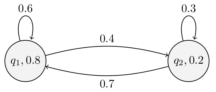
(a) Context model

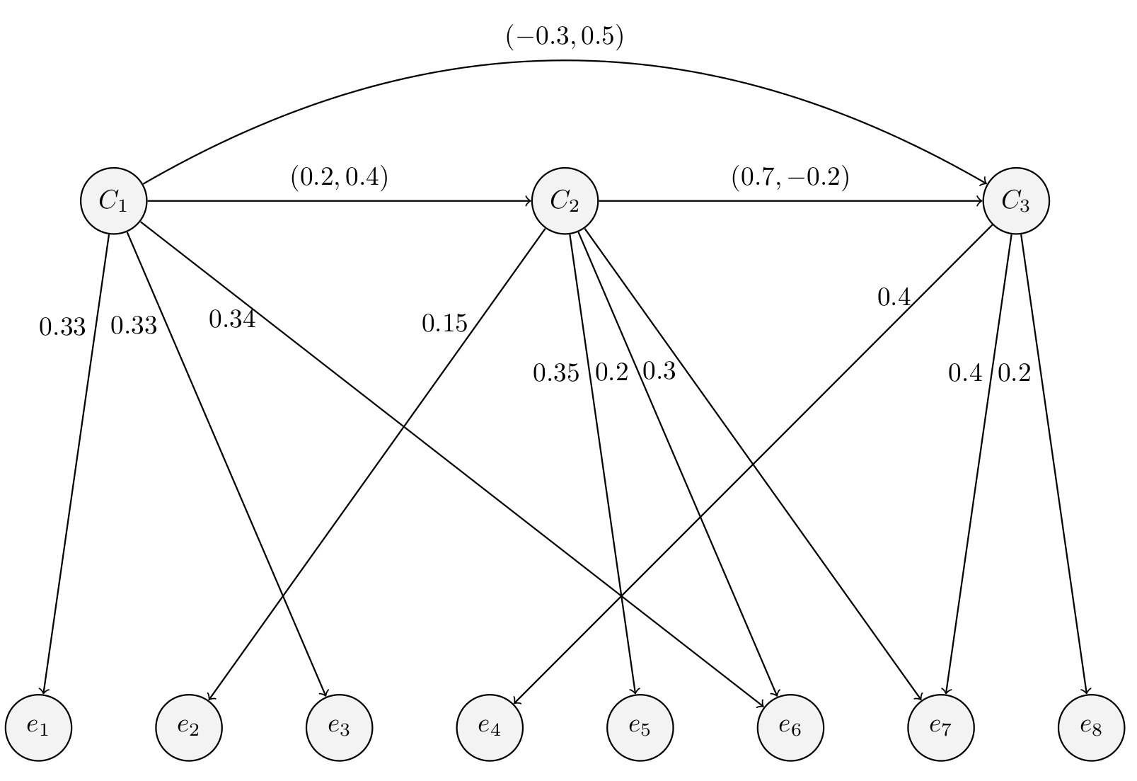
(b) Conceptual knowledge model

	$(C_{1},C_{2})$	$(C_{2},C_{3})$	$(C_{1},C_{3})$
$i=1$	$0.35$	$0.2$	$0.45$
$i=2$	$0.15$	$0.6$	$0.25$

(c) Concept pair generation probability as per context

Figure 2: Illustrative Data

2.2 Modeling conceptual knowledge.

We assume that the expert’s domain-specific conceptual knowledge consists of three components: (i) a set $\mathcal{E}$ of entities in the given domain, (ii) a set $\mathcal{C}$ of concepts in the given domain along with relations $\mathcal{R}$ among them, and (iii) membership probabilities of these entities in various concepts.

1. Entities. We assume that, for some integer $n$, the expert is aware of $n$ entities $\mathcal{E}=\{e_{1},e_{2},\ldots,e_{n}\}$ in her domain.

2. Concepts and relations among them. We assume that, for some integer $k$ ($k$ is usually much smaller than $n$), the expert is aware of $k$ concepts $\mathcal{C}=\{C_{1},C_{2},\ldots,C_{k}\}$ in her domain.

   Further, we assume that the expert has knowledge of $r$ relations among pairs of these concepts. We model this by a set $\mathcal{R}\subseteq\mathcal{C}\times\mathcal{C}$ of size $r$. In our model, every ordered pair $(C_{j_{1}},C_{j_{2}})\in\mathcal{R}$ is labeled with a $d$-dimensional vector ${\bf v}_{j_{1}j_{2}}$ describing the nature of the relation from concept $C_{j_{1}}$ to concept $C_{j_{2}}$.

3. Membership of entities in various concepts. We assume that for every concept-entity pair $(C_{i},e_{j})$, $1\leq i\leq k$ and $1\leq j\leq n$, our model has a probability $q_{ij}$, $0\leq q_{ij}\leq 1$, of entity $e_{j}$ being an instance of concept $C_{i}$. Note that, because of the probabilistic nature of our document generation model, we have the constraints that $\sum_{j=1}^{n}q_{ij}=1$ for all $1\leq i\leq n$.

Example. Figure 2(b) shows an expert’s conceptual knowledge with three concepts and eight entities. There are a total of $3$ relations in set $\mathcal{R}$, which are shown by directed arrows between concepts. Further, the probability $q_{ij}$, where $1\leq i\leq 3$ and $1\leq j\leq 8$, is shown alongside the arrow from node representing concept $C_{i}$ to node representing entity $e_{j}$. (The absence of an arrow from $C_{i}$ to $e_{j}$ denotes that $q_{ij}=0$.)

We assume that the relations between concept pairs in $\mathcal{R}$ are encoded by real vectors of dimension $d=2$. The vector ${\bf v}_{j_{1}j_{2}}$ corresponding to concept pair $(C_{j_{1}},C_{j_{2}})\in\mathcal{R}$ is shown alongside the arrow from node $C_{j_{1}}$ to node $C_{j_{2}}$.

2.3 Modeling document generation.

We make the assumption that the expert first picks a relation from the set $\mathcal{R}$ of relations among high-level concepts based on the current context, and then proceeds from the high-level conceptual relation to a low-level specific entity-relation triple. The overall schema of our document generation consists of cyclic repetition of these three steps (see Figure 3) for each sentence written by the expert:

1. updating of current context as per $\mathcal{M}$,

2. generating a conceptual pair $(C_{j_{1}},C_{j_{2}})\in\mathcal{R}$ based on current context, and

3. instantiating the above concept pair to an entity-level relation $(e_{x},{\bf r},e_{y})$ based on the conceptual knowledge model.

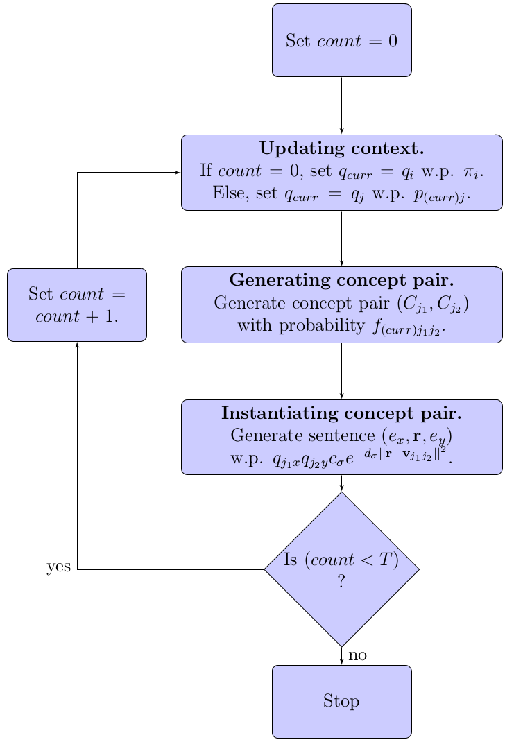
Figure 3: Flowchart of document generation

As noted above, in between successive sentences generated in the above manner, the current context changes in the first step according to the discrete Markov process $\mathcal{M}$. The second step in the above cycle is called concept pair generation and the third step is called concept pair instantiation. We now describe these later two steps in detail.

1. Concept pair generation. In this step, based on the current context $q_{curr}$, the expert probabilistically picks one of the relations $(C_{j_{1}},C_{j_{2}})$ from the set of relations $\mathcal{R}$ among domain concepts.

   To model the dependence of generated concept pair on current context, we add probabilities $f_{ij_{1}j_{2}}$ to our model, where $1\leq i\leq b$, $1\leq j_{1},j_{2}\leq k$ and $j_{1}\neq j_{2}$. $f_{ij_{1}j_{2}}$ denotes the probability of the expert generating concept pair $(C_{j_{1}},C_{j_{2}})\in\mathcal{R}$ when the current context is $q_{i}$. Thus, an expert with context $q_{curr}$ will generate $(C_{j_{1}},C_{j_{2}})\in\mathcal{R}$ with probability $f_{(curr)j_{1}j_{2}}$. The reader is referred to Table I for constraints satisfied by this set of parameters.

2. Concept pair instantiation. In this step, first concept $C_{j_{1}}$ is instantiated to entity $e_{x}$ with probability $q_{j_{1}x}$. Next, second concept $C_{j_{2}}$ is instantiated to entity $e_{y}$ with probability $q_{j_{2}y}$. Finally, the relation $\bf{v}_{j_{1}j_{2}}$ between $C_{j_{1}}$ and $C_{j_{2}}$ leads to relation ${\bf r}$ between $e_{x}$ and $e_{y}$ with probability $c_{\sigma}e^{-d_{\sigma}||{\bf r}-{\bf v}_{j_{1}j_{2}}||^{2}}$, where $c_{\sigma}=\frac{1}{(2\pi\sigma^{2})^{d/2}}$ and $d_{\sigma}=\frac{1}{2\sigma^{2}}$.

Example. We complete our example depicted in Figure 2 by listing, for all $1\leq i\leq 2$ and $(C_{j_{1}},C_{j_{2}})\in\mathcal{R}$, the probabilities $f_{ij_{1}j_{2}}$ of generating concept pair $(C_{j_{1}},C_{j_{2}})$ when in state $q_{i}$ of $\mathcal{M}$.

Suppose a document ${\bf O}$ consists of the following five sentences: $(e_{2},(0.9,-0.1),e_{7})$, $(e_{3},(0.5,0.3),e_{7})$, $(e_{1},(0.1,0.7),e_{6})$, $(e_{1},(-0.4,0.6),e_{8})$, and $(e_{3},(-0.1,0.2),e_{4})$. Then, the probability that $\mathcal{D}$ is generated by our example model (for $\sigma=0.1$) can be calculated using the equations in Section $3.3$ and is approximately equal to $2.15496\times 10^{-11}$. (Note that this is actually the value of a probability density function and hence can be greater than $1$ in some cases.)

3 Maximum likelihood principle: Using Baum-Welch

In the following, we use the notation of Rabiner’s HMM tutorial [8].

3.1 HMM $\mathcal{H}$

We start by noting that our document generation model is equivalent to a single Hidden Markov Model $\mathcal{H}$ with the following description:

1. There are a total of $N=bk(k-1)$ states in $\mathcal{H}$. The states of $\mathcal{H}$ are indexed by $3$-tuples $(j,l_{1},l_{2})$, where $1\leq j\leq b$, $1\leq l_{1},l_{2}\leq k$, and $l_{1}\neq l_{2}$.

2. The observations (or, outputs) of $\mathcal{H}$ consist of a sequence of elements from the set

   $$\mathcal{O}=\{(e_{x},\vec{r},e_{y})~{}|~{}1\leq x,y\leq n~{}and~{}\vec{r}\in\mathcal{V}\}$$

   Here $\mathcal{V}$ denotes the set of $d$-dimensional real vectors.

3. The transition probability $a_{(j,l_{1},l_{2})(j^{\prime},l^{\prime}_{1},l^{\prime}_{2})}$ from state $(j,l_{1},l_{2})$ to state $(j^{\prime},l^{\prime}_{1},l^{\prime}_{2})$ is given by the expression:

   $$a_{(j,l_{1},l_{2})(j^{\prime},l^{\prime}_{1},l^{\prime}_{2})}=p_{jj^{\prime}}f_{j^{\prime}l^{\prime}_{1}l^{\prime}_{2}}$$

   We use $A$ to denote the state transition probability matrix.

4. The probability $b_{(j,l_{1},l_{2})}$ of observing $(e_{x},\vec{r},e_{y})\in\mathcal{O}$ in state $(j,l_{1},l_{2})$ is given by:

   $$b_{(j,l_{1},l_{2})}((e_{x},\vec{r},e_{y}))=q_{l_{1}x}q_{l_{2}y}c_{\sigma}e^{-d_{\sigma}||\vec{r}-{\bf v}_{l_{1}l_{2}}||^{2}}$$

5. Finally, the probability $\pi_{(j,l_{1},l_{2})}$ that $(j,l_{1},l_{2})$ is the first state of $\mathcal{H}$ is given by the expression:

   $$\pi_{(j,l_{1},l_{2})}=\pi_{j}f_{jl_{1}l_{2}}$$

   Note that the parameter $\pi_{(j,l_{1},l_{2})}$ on the left hand side denotes the stationary probability of state $(j,l_{1},l_{2})$ in HMM $\mathcal{H}$, whereas the parameter $\pi_{j}$ on the right hand side denotes the stationary probability of $\mathcal{M}$ discussed in Table I.

3.2 Problem Formulation

As in [8], we use $\lambda$ to denote the model parameters of HMM $\mathcal{H}$. Further, we use ${\bf O}=\{O_{1},O_{2},\ldots,O_{T}\}$ to denote a particular observation sequence (or, equivalently the document generated), where $O_{t}=(e_{i_{t}},{\bf r}_{t},e_{j_{t}})$ for $1\leq t\leq T$.

Our objective is to find model parameters which maximize the probability of generating observation sequence ${\bf O}$ (see Problem 3 in [8]). In other words, we want to find model parameters $\lambda^{*}$ such that:

$$P({\bf O}~{}|~{}\lambda^{*})=max_{\lambda}P({\bf O}~{}|~{}\lambda)$$

We use $Q$ to denote a sequence $q_{1}=(s_{1},a_{1},b_{1}),q_{2}=(s_{2},a_{2},b_{2}),\ldots,q_{T}=(s_{T},a_{T},b_{T})$ of states of $\mathcal{H}$.

3.3 Forward and Backward Variables

We now define forward variable $\alpha_{t}((j,l_{1},l_{2}))$ (see equation $(18)$ in [8]) as:

$$\alpha_{t}((j,l_{1},l_{2}))=P(O_{1},O_{2},\ldots,O_{t},q_{t}=(j,l_{1},l_{2})~{}|~{}\lambda)$$

By applying equations $(19)$ and $(20)$ of [8] to HMM $\mathcal{H}$, we obtain inductive equations for the forward variables.

$$\alpha_{1}((j,l_{1},l_{2}))=\pi_{j}f_{jl_{1}l_{2}}q_{l_{1}i_{1}}q_{l_{2}j_{1}}c_{\sigma}e^{-d_{\sigma}||{\bf r}_{1}-\vec{v}_{l_{1}l_{2}}||^{2}}$$

Further, for $2\leq t\leq T$:

$$\alpha_{t}((j,l_{1},l_{2}))=\sum_{(j^{\prime},l^{\prime}_{1},l^{\prime}_{2})}\alpha_{t-1}((j^{\prime},l^{\prime}_{1},l^{\prime}_{2}))p_{j^{\prime}j}f_{jl_{1}l_{2}}q_{l_{1}i_{t}}q_{l_{2}j_{t}}c_{\sigma}e^{-d_{\sigma}||{\bf r}_{t}-\vec{v}_{l_{1}l_{2}}||^{2}}$$

Backward variable $\beta_{t}((j,l_{1},l_{2}))$ is defined as follows (see equation $(23)$ in [8]):

$$\beta_{t}((j,l_{1},l_{2}))=P(O_{t+1},O_{t+2},\ldots,O_{T}~{}|~{}q_{t}=(j,l_{1},l_{2}),~{}\lambda)$$

The inductive equations for the backward variables are then obtained using equations $(24)$ and $(25)$ in [8].

$$\beta_{T}((j,l_{1},l_{2}))=1$$

Further, for $t=T-1,T-2,\ldots,1$:

$$\beta_{t}((j,l_{1},l_{2}))=\sum_{(j^{\prime},l^{\prime}_{1},l^{\prime}_{2})}p_{jj^{\prime}}f_{j^{\prime}l^{\prime}_{1}l^{\prime}_{2}}q_{l^{\prime}_{1}i_{t+1}}\\ q_{l^{\prime}_{2}j_{t+1}}c_{\sigma}e^{-d_{\sigma}||{\bf r}_{t+1}-\vec{v}_{l^{\prime}_{1}l^{\prime}_{2}}||^{2}}\beta_{t+1}((j^{\prime},l^{\prime}_{1},l^{\prime}_{2}))$$

3.4 Probability of being in a state or making a particular transition

Following [8], let $\gamma_{t}((j,l_{1},l_{2}))$ denote the probability:

$$\gamma_{t}((j,l_{1},l_{2}))=P(q_{t}=(j,l_{1},l_{2})~{}|~{}{\bf O},\lambda)$$

By equation $(27)$ in [8], for $1\leq t\leq T$:

$$\gamma_{t}((j,l_{1},l_{2}))=\frac{\alpha_{t}((j,l_{1},l_{2}))\beta_{t}((j,l_{1},l_{2}))}{\sum_{(j^{\prime},l^{\prime}_{1},l^{\prime}_{2})}\alpha_{t}((j^{\prime},l^{\prime}_{1},l^{\prime}_{2}))\beta_{t}((j^{\prime},l^{\prime}_{1},l^{\prime}_{2}))}$$

Proceeding further, for $1\leq t\leq T-1$, let $\xi_{t}((j,l_{1},l_{2}),(j^{\prime},l^{\prime}_{1},l^{\prime}_{2}))$ denote the probability $P(q_{t}=(j,l_{1},l_{2}),q_{t+1}=(j^{\prime},l^{\prime}_{1},l^{\prime}_{2})~{}|~{}{\bf O},\lambda)$.

Applying equation $(37)$ from [8] to $\mathcal{H}$, we obtain:

$$\xi_{t}((j,l_{1},l_{2}),(j^{\prime},l^{\prime}_{1},l^{\prime}_{2}))=\frac{\alpha_{t}((j,l_{1},l_{2}))p_{jj^{\prime}}f_{j^{\prime}l^{\prime}_{1}l^{\prime}_{2}}q_{l^{\prime}_{1}i_{t+1}}q_{l^{\prime}_{2}j_{t+1}}c_{\sigma}e^{-d_{\sigma}||{\bf r}_{t+1}-{\bf v}_{l^{\prime}_{1}l^{\prime}_{2}}||^{2}}\beta_{t+1}((j^{\prime},l^{\prime}_{1},l^{\prime}_{2}))}{P({\bf O}~{}|~{}\lambda)}$$ (1)

Finally, note that by equation $(21)$ of [8], the denominator in the above expression is equal to:

$$P({\bf O}~{}|~{}\lambda)=\sum_{(j,l_{1},l_{2})}\alpha_{T}((j,l_{1},l_{2}))$$

3.5 Wildcard characters

In the following section, the wildcard character ‘*’ denotes summation over the corresponding index. Thus, for example:

$$\gamma_{t}((j,*,*))=\smashoperator[]{\sum_{\{l_{1},l_{2}~{}|~{}l_{1}\neq l_{2},~{}1\leq l_{1},l_{2}\leq k\}}^{}}\gamma_{t}((j,l_{1},l_{2}))$$

$$\gamma_{t}((*,l_{1},*))=\smashoperator[]{\sum_{\{j,l_{2}~{}|~{}1\leq j\leq b,~{}1\leq l_{2}\leq k,~{}l_{1}\neq l_{2}\}}^{}}\gamma_{t}((j,l_{1},l_{2}))$$

$$\xi_{t}((j,*,*),(j^{\prime},*,*))=\sum_{\begin{subarray}{c}\{l_{1},l_{2}~{}|\quad\\ ~{}l_{1}\neq l_{2},\\ ~{}1\leq l_{1},\\ l_{2}\leq k\}\end{subarray}}\smashoperator[]{\sum_{\begin{subarray}{c}\{l^{\prime}_{1},l^{\prime}_{2}~{}|\\ ~{}l^{\prime}_{1}\neq l^{\prime}_{2},\\ ~{}1\leq l^{\prime}_{1},\\ l^{\prime}_{2}\leq k\}\end{subarray}}^{}}\xi_{t}((j,l_{1},l_{2}),(j^{\prime},l^{\prime}_{1},l^{\prime}_{2}))$$

3.6 Reestimation / update equations

We now describe the reestimation equations for $\mathcal{H}$. These equations can be derived by optimizing Baum’s auxiliary function (see equation $(42)$ in [8]) using the method of Lagrange multipliers. The derivation of these reestimation equations is given in the appendix.

$$\overline{\pi}_{i}=\gamma_{1}((i,*,*))~{},1\leq i\leq b$$

$$\overline{p}_{j_{1}j_{2}}=\frac{\sum_{t=1}^{T-1}\xi_{t}((j_{1},*,*),(j_{2},*,*))}{\sum_{t=1}^{T-1}\gamma_{t}((j_{1},*,*))}~{},1\leq j_{1},j_{2}\leq b$$

$$\overline{f}_{jl_{1}l_{2}}=\frac{\sum_{t=1}^{T}\gamma_{t}((j,l_{1},l_{2}))}{\sum_{t=1}^{T}\gamma_{t}((j,*,*))}~{},1\leq j\leq b,~{}1\leq l_{1},l_{2}\leq k,\\ ~{}and~{}l_{1}\neq l_{2}$$

$$\overline{q}_{xy}=\frac{\sum_{t~{}|~{}i_{t}=y}\gamma_{t}((*,x,*))+\sum_{t~{}|~{}j_{t}=y}\gamma_{t}((*,*,x))}{\sum_{t=1}^{T}\gamma_{t}((*,x,*))+\sum_{t=1}^{T}\gamma_{t}((*,*,x))}~{},\\ 1\leq x\leq k,1\leq y\leq n$$

$$\overline{{\bf v}}_{l_{1},l_{2}}=\frac{\sum_{t=1}^{T}{\bf r}_{t}\cdot\gamma_{t}((*,l_{1},l_{2}))}{\sum_{t=1}^{T}\gamma_{t}((*,l_{1},l_{2}))}~{},1\leq l_{1},l_{2}\leq k$$

3.7 Algorithm Outline

We start with random starting model parameters $\lambda^{0}$. Further, we choose an error limit $\epsilon>0$.

We stop updating the model parameters at time $t+1$ iff $||\lambda^{t+1}-\lambda^{t}||<\epsilon$. Here $\lambda^{t}$ denotes the model parameter values after $t$ iterations of Baum-Welch updation.

3.8 Basic code optimizations

We do the following optimizations which significantly decrease the running time of our code:

1. Multiprocessing. We build support for multiprocessing in our code. In particular, for a fixed $t$, the calculation of the set of quantities $\{\alpha_{t}((j,l_{1},l_{2}))~{}|~{}1\leq j\leq b,1\leq l_{1},l_{2}\leq k,l_{1}\neq l_{2}\}$ can be completely parallelized.

2. Fast calculation of $\xi_{t}((j_{1},*,*),(j_{2},*,*))$. We observe that the update equations for the parameters of our model only use the values $\xi_{t}((j_{1},*,*),(j_{2},*,*))$ for $1\leq j_{1},j_{2}\leq k$. We give a procedure to compute these quantities which is faster than the standard procedure.

3. Memoization. We avoid re-computation by storing our results in a lookup table.

3.9 Finding relevant relation between the concept pairs

Note that, not counting self-loops, our model parameters assume that all $k(k-1)$ possible concept pairs among the $k$ concepts exist in the conceptual graph. However, in general, in any domain-specific conceptual graph only a subset of these concept pairs will be present.

We fix a positive real threshold $0<\theta\leq T$. Further, we say that a given concept pair $(l_{1},l_{2})$ is relevant iff the quantity $S(l_{1},l_{2})=\sum_{t=1}^{T}\gamma_{t}(*,l_{1},l_{2})$ is at least $\theta$.

Observe that $S(l_{1},l_{2})$ is the expected number of times the HMM $\mathcal{H}$ visits a state of the form $(j,l_{1},l_{2})$ where $1\leq j\leq b$, given that the observations made are ${\bf O}$ and model parameters are $\lambda$. From the above, we can further note that

$$\sum_{(l_{1},l_{2})~{}|~{}l_{1}\neq l_{2}~{}and~{}1\leq l_{1},l_{2}\leq k}S(l_{1},l_{2})$$

is exactly $T$.

In the following, we assume that only relevant concept pairs exist in the document writer’s conceptual graph. The irrelevant concept pairs are discarded from further consideration.

4 Experimentation and Analysis

In this section we discuss our experimental setup, introduce evaluation parameters, measure the performance of our algorithm on various data-sets and finally make observations regarding the nature of results obtained.

4.1 Experimental Setup

We implemented our model on different natural language texts and carried out a detailed analysis of the conceptualizations generated. All of the input texts pertain to software engineering domain, though we believe that natural language text from any other domain will yield comparable results.

To obtain the intermediate knowledge graph (see first step in Fig. 1) from natural language text, we make use of the well-known textrank[9] technique to extract keywords from each project description. These keywords are then used with NLTK-POS taggers [10] to form entities and their inter-relations in the knowledge graph.

Although we use a basic methodology to extract knowledge graph from natural language text, our algorithm (see Section 3) is shown to perform well even with this basic method. Hence, we firmly believe that better results would be obtained by more sophisticated knowledge graph construction techniques.

4.2 Performance measures for knowledge graph conceptualization

Let $\mathcal{C}^{A}$ be the conceptualized knowledge graph returned by running our algorithm on input. Suppose $\mathcal{C}^{A}$ has $k_{1}$ concepts $C_{1}^{A},C_{2}^{A},\ldots,C_{k_{1}}^{A}$. Let $I_{1}\subseteq\{(i,j)~{}|~{}1\leq i,j\leq k_{1}~{}and~{}i\neq j\}$ be the set of ordered pairs of concepts which have a relation between them in $\mathcal{C}^{A}$. Finally, for $(i,j)\in I_{1}$, let $\vec{r}_{ij}$ denote the relation vector from concept $C_{i}^{A}$ to $C_{j}^{A}$.

On the other hand, let $\mathcal{C}^{S}$ be the silver standard supplied by experts. Let $C_{1}^{S},C_{2}^{S},\ldots,C_{k_{2}}^{S}$ be the concepts in $\mathcal{C}^{S}$ and let $I_{2}\subseteq\{(i^{\prime},j^{\prime})~{}|~{}1\leq i^{\prime},j^{\prime}\leq k_{2}~{}and~{}i^{\prime}\neq j^{\prime}\}$ be the set of ordered pairs of concepts which admit a relation in $\mathcal{C}^{S}$. We use $\vec{t}_{i^{\prime}j^{\prime}}$ to denote the relation vector from concept $C_{i^{\prime}}^{S}$ to $C_{j^{\prime}}^{S}$.

Note that the concepts given by the experts are subsets of the entity set $\mathcal{E}$ and require no further modification. However, the concepts generated by our algorithm are not proper subsets of $\mathcal{E}$ and instead have instantiation probabilities for each entity. To take care of this, in the following, we fix a cutoff value $\vartheta$ between $0$ and $1$, and use concept $C_{i}^{A}$ to denote the set $\{e_{j}~{}|~{}q_{ij}\geq\vartheta\}$. (Here, as in the algorithm description above, $q_{ij}$ denotes the probability of instantiating entity $e_{j}$ from concept $C_{i}^{A}$.)

Our measures are based on the well-known notions of precision, recall, and $F_{1}$ score.

For $1\leq i\leq k_{1}$ and $1\leq j^{\prime}\leq k_{2}$, the quantities $p(C_{i}^{A},C_{j^{\prime}}^{S})$ (similar to precision), $r(C_{i}^{A},C_{j^{\prime}}^{S})$ (similar to recall), and $f(C_{i}^{A},C_{j^{\prime}}^{S})$ (similar to $F_{1}$ score) are defined as follows:

$$p(C_{i}^{A},C_{j^{\prime}}^{S})=\frac{|C_{i}^{A}\bigcap C_{j^{\prime}}^{S}|}{|C_{i}^{A}|}$$

$$r(C_{i}^{A},C_{j^{\prime}}^{S})=\frac{|C_{i}^{A}\bigcap C_{j^{\prime}}^{S}|}{|C_{j^{\prime}}^{S}|}$$

$$f(C_{i}^{A},C_{j^{\prime}}^{S})=\frac{2\cdot p(C_{i}^{A},C_{j^{\prime}}^{S})\cdot r(C_{i}^{A},C_{j^{\prime}}^{S})}{p(C_{i}^{A},C_{j^{\prime}}^{S})+r(C_{i}^{A},C_{j^{\prime}}^{S})}$$

Note that all three of the above quantities are real numbers between $0$ and $1$. Further, $f(C_{i}^{A},C_{j^{\prime}}^{S})$ can be called the closeness between concepts $C_{i}^{A}$ (generated by our algorithm) and $C_{j^{\prime}}^{S}$ (part of the silver standard).

4.2.1 Case I: The silver standard consists only of concepts without any relations between them

First, we consider the case when the silver standard supplied by the experts only has concepts and no relations among them. In this case, we define the following three quantities, which can be seen as defining notions of precision, recall, and $F_{1}$ score between the computed conceptualization $\mathcal{C}^{A}$ and the conceptualization $\mathcal{C}^{S}$ generated by experts:

$$p^{(I)}(\mathcal{C}^{A},\mathcal{C}^{S})=\frac{\sum_{i=1}^{k_{1}}\left(\max_{1\leq j^{\prime}\leq k_{2}}f(C_{i}^{A},C_{j^{\prime}}^{S})\right)}{k_{1}}$$

$$r^{(I)}(\mathcal{C}^{A},\mathcal{C}^{S})=\frac{\sum_{j^{\prime}=1}^{k_{2}}\left(\max_{1\leq i\leq k_{1}}f(C_{i}^{A},C_{j^{\prime}}^{S})\right)}{k_{2}}$$

$$f^{(I)}(\mathcal{C}^{A},\mathcal{C}^{S})=\frac{2\cdot p^{(I)}(\mathcal{C}^{A},\mathcal{C}^{S})\cdot r^{(I)}(\mathcal{C}^{A},\mathcal{C}^{S})}{p^{(I)}(\mathcal{C}^{A},\mathcal{C}^{S})+r^{(I)}(\mathcal{C}^{A},\mathcal{C}^{S})}$$

A value of $f^{(I)}(\mathcal{C}^{A},\mathcal{C}^{B})$ close to $1$ implies that our conceptualization is very close to experts’ conceptual knowledge.

4.2.2 Case II: The silver standard has both concepts as well as relations between them

Given two relations $\mathcal{R}_{ij}=(C_{i}^{A},C_{j}^{A},\vec{r}_{ij})$ and $\mathcal{T}_{i^{\prime}j^{\prime}}=(C_{i^{\prime}}^{S},C_{j^{\prime}}^{S},\vec{t}_{i^{\prime}j^{\prime}})$ where $(i,j)\in I_{1}$ and $(i^{\prime},j^{\prime})\in I_{2}$, we define the closeness between these two relations by the quantity:

$$g(\mathcal{R}_{ij},\mathcal{T}_{i^{\prime}j^{\prime}})=HM(f(C_{i}^{A},C_{i^{\prime}}^{S}),f(C_{j}^{A},C_{j^{\prime}}^{S}),e^{-d(\vec{r}_{ij},\vec{t}_{i^{\prime}j^{\prime}})})$$

Here $HM(x_{1},x_{2},x_{3})=\frac{3}{\frac{1}{x_{1}}+\frac{1}{x_{2}}+\frac{1}{x_{3}}}$ denotes the harmonic mean of $x_{1}$, $x_{2}$ and $x_{3}$ and $d(\vec{r}_{ij},\vec{t}_{i^{\prime}j^{\prime}})$ denotes Euclidean distance between corresponding vectors.

We now define quantities similar to precision and recall when the relations present in $\mathcal{C}^{A}$ are compared with the relations present in $\mathcal{C}^{B}$:

$$p^{(II)}(\mathcal{C}^{A},\mathcal{C}^{B})=\frac{\sum_{(i,j)\in I_{1}}\max_{(i^{\prime},j^{\prime})\in I_{2}}g(\mathcal{R}_{ij},\mathcal{T}_{i^{\prime}j^{\prime}})}{|I_{1}|}$$

$$r^{(II)}(\mathcal{C}^{A},\mathcal{C}^{B})=\frac{\sum_{(i^{\prime},j^{\prime})\in I_{2}}\max_{(i,j)\in I_{1}}g(\mathcal{R}_{ij},\mathcal{T}_{i^{\prime}j^{\prime}})}{|I_{2}|}$$

Finally, the $F_{1}$ score between $\mathcal{C}^{A}$ and $\mathcal{C}^{B}$ is given, as above, by:

$$f^{(II)}(\mathcal{C}^{A},\mathcal{C}^{S})=\frac{2\cdot p^{(II)}(\mathcal{C}^{A},\mathcal{C}^{S})\cdot r^{(II)}(\mathcal{C}^{A},\mathcal{C}^{S})}{p^{(II)}(\mathcal{C}^{A},\mathcal{C}^{S})+r^{(II)}(\mathcal{C}^{A},\mathcal{C}^{S})}$$

We would ideally like our algorithm to generate conceptualizations for which the $F_{1}$ score is as close to $1$ as possible.

4.3 Analysis

We now evaluate the output obtained by our methodology w.r.t. performance measures defined in previous section. The results obtained are compared with a silver standard. The silver standard is created by two domain experts independently. Wherever the concepts or relations created by two experts differed the authors made the final call by referring to other sources.

4.3.1 Quantitative Analysis

We crawled the freely available online descriptions of Apache ACE, Apache Avro, Apache XMLBeans and Microsoft Azure Database. Once the knowledge graph is obtained, we conceptualize it by our proposed algorithm. We check the efficacy of results using a silver standard.

Crawled Project Descriptions	No. of Relations ($T$)	$\sigma$	No. of Markov States (parameter $b$)	No. of Concepts (parameter $k$)	$f^{(I)}(\mathcal{C}^{A},\mathcal{C}^{S})$	$f^{(II)}(\mathcal{C}^{A},\mathcal{C}^{S})$
Apache Avro	$10$	$0.05$	$3$	$3$	$0.387$	$0.227$
Microsoft Azure	$100$	$0.01$	$7$	$30$	$0.302$	$0.317$
Microsoft Azure	$200$	$0.1$	$10$	$50$	$0.437$	$0.411$
Apache Avro $\&$ Apache ACE $\&$ Apache XML Beans	$800$	$0.1$	$15$	$80$	$0.717$	$0.533$

TABLE II: Performance of the Proposed Model on various software documentations

Table II depicts performance of our model for texts obtained from different sources (Column 1) with different number of relations (Column 2) in the knowledge graphs constructed from respective texts. As the number of relations increase in the constructed knowledge graph, we also increase the corresponding Markov states (Column 4) and number of concepts for output (Column 5). In each case, we run the algorithm with $10$ different random initial values of the model parameters and populate Columns 6 and 7 using the best answer as per closeness of results w.r.t. silver standard.

Few observation that can be derived from Table II are:

• For all our experiments, our model achieves reasonably high values of evaluation parameters $f^{I}(\mathcal{C}^{A},\mathcal{C}^{S})$ and $f^{II}(\mathcal{C}^{A},\mathcal{C}^{S})$ (tabulated in Columns 6 and 7 of Table II). This depicts the considerable accuracy achieved by our simple algorithm.

• For all our experiments, we get better results for $f^{(I)}(\mathcal{C}^{A},\mathcal{C}^{S})$ when compared with $f^{(II)}(\mathcal{C}^{A},\mathcal{C}^{S})$. This is most probably because incorporating the quality of conceptual relations generated in the evaluation parameter makes it more stringent.

• Note that our algorithm seems to perform increasingly well on the evaluation parameters as the number of relations in input knowledge graph increases. Since our method has statistical underpinnings, a larger data-set seems to allow it to learn conceptual knowledge with greater certainty and clarity. Further, since we essentially model the mental processes of a domain expert, the above mentioned behaviour of our algorithm corresponds well with the everyday notion that a more widely-read expert will usually have better conceptual knowledge about the domain.

• We increase the value of the variance parameter $\sigma$ as the number of relations in the input knowledge graph increase. This increase in $\sigma$ leads to an increasingly “coarser” fitting of conceptual knowledge over the input knowledge graph. This allows for a graceful variation in the generation of entity-level relations in the input knowledge graph during instantiation from respective conceptual relations.

4.3.2 Qualitative Analysis

We now discuss the quality of conceptualizations obtained by our algorithm on a particular document. This document was created after crawling and pre-processing description of “Microsoft Azure SQL Database” available on-line. The exact natural language text document, which was used to construct the knowledge graph, is available at - goo.gl/YZt3Eh. We note that only the first $100$ relations, extracted while constructing the knowledge graph, were subsequently given as input to our conceptualization algorithm.

Figure 4 depicts a portion of the conceptualization obtained via our algorithm. Each circle depicts a concept and the extracted entities comprising a particular concept. The entities in the concepts are written in decreasing order of their membership probabilities in that particular concept. For example, in Concept 1, the entity “databases” has the highest membership probability whereas the entity “small single databases” has the lowest membership probability. (Only entities with significant membership probabilities are considered to belong to a given concept.) Finally, the relevant relations shown between the concepts were found by the method discussed in Section 3.9.

Few observations to be made from Figure 4 are as follows.

• Most of the concepts obtained by our algorithm are cogent and convincing. For example, Concept 0 groups together all entities referring to “databases” in one or the other way. Similarly, Concept 4 enumerates several “application areas” for databases and Concept 6 lists out several “desirable attributes”.

• In terms of relations between different concepts, note that Concept 0 has an edge to Concept 4 with label “for” and further, Concept 4 has an edge to Concept 6 with label ”to ensure”. Intuitively, this means that “databases” are used for “application areas”, each of which must incorporate certain “desirable attributes”.

• Our results are noteworthy because they have been obtained without using any lexical or semantic similarities between entity labels.

• As a limitation, we note that entities such as “app”, “global network”, “world”, “pool”, etc. have been grouped together in Concept 1. This can be considered a bit vague as these entities are very generic and do not combine together into a domain concept. Certainly, in such cases we require more information to gauge the validity of the results.

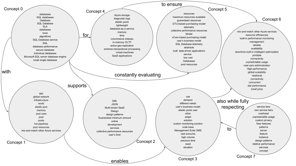
Figure 4: Example– Conceptualized Knowledge Graph

We firmly believe that output quality can further increase on a more accurate knowledge graph obtained from natural language text. A simplistic automation of this step in our experiments leads to some generic entities and avoidable errors in the input knowledge graph, thus leading to few incorrect conceptualizations.

5 Related Work

We discuss relevant literature from three different aspects: (i) concept extraction, (ii) ontology learning, and (iii) knowledge graph construction and refinement. We note that these three aspects are not mutually exclusive and share common methodologies.

Our discussion of these three aspects is motivated by following two reasons:

1. First, to the best of our knowledge, a single, unified method to accomplish exactly the task outlined in this paper has not yet been discussed in literature. Hence, we are constrained to discuss previous work in well-researched related areas, which address problems of a similar flavour.

2. Secondly, our model can be used as an integral component for automating different tasks in each of these three aspects, and in this sense, forms a significant contribution to current work in each of these three areas.

5.1 Concept/Terminology Extraction

Concept extraction from unstructured documents is a well-known and vast area of research. Various systems and/or system components have been built and evaluated for this particular task (see Section 3 in [11] for a recent survey of such works in reference to Semantic Web). Additionally, some tools not covered in [11], such as CFinder [12], KP-Miner [13], and Moki [14] exist for concept extraction. CFinder claims to have favorable performance when compared with three other well-known systems: Text2Onto [15], KP-Miner [13], and Moki [14]. Further, systems such as those in [16, 17], also achieve the additional task of finding various relations among the extracted concepts.

In addition to being useful on their own, concept extraction methods are often used as a component in several systems for large-scale ontology population and learning (see [18]), which we discuss next.

5.2 Ontology learning from text

Natural language text to ontology is a well researched area known as Ontology learning and population (OL&P). OL&P is a complex task consisting more or less of the following generic steps: (i) extracting domain relevant terms, (ii) identifying and labeling domain specific concepts, (iii) extracting both taxonomic and non-taxonomic relations among the domain concepts, and (iv) extracting logical rules and frameworks satisfied by the various concepts (see [19, 18]).

OL&P researchers have used natural language processing, machine learning, logic-based, and various other techniques to achieve their respective goals [18][20][21][22]. Some of the OL&P systems are [23, 24, 25, 26].

However, all current methods suffer from the drawback that their design consists of a composition of several smaller components for very basic tasks, with each component using only fundamental techniques. In contrast, our method spans several layers of the “ontology layer cake” (see [19] for definition of this term).

In addition to the above, see [4] for a discussion of abstraction networks for existing ontologies in the medical domain.

5.3 Knowledge Graph Construction and Refinement

Knowledge graphs can be categorized on different dimensions: (a) The way they have been constructed (automatically or manually) (b) Generic or Domain-Specific (c) The source of their data (Semantic Web or an organization) etc. [1].

We discuss few recent or seminal contributions concerned with knowledge graph identification, construction and abstraction. [27] provides a model to represent entity relation pair as unique vector. It is computationally expensive and requires large amount of training for varied domains. Particularly, graph abstraction is proposed in [5] where the authors use graph structure and graph-theoretic measures to store and query graph in an efficient manner. In [3] Probabilistic Soft Logic is used to reduce errors in a graph extracted from natural language text and uses other graphs to assist in this cleaning. Pujara et al.[3] use Probabilistic Soft Logic for the problem of “knowledge graph identification”. To be more specific, given a corpus of extracted entities and relations, they first use modeling followed by inference in Probabilistic Soft Logic to come up with the most likely probabilistic confidence values for the given set of nodes and relations. Next, they round these confidence values using a fixed threshold to identify a consistent knowledge graph from the extracted corpus. Further, in [28], they show that graph partitioning techniques with parallel processing can significantly reduce the running time of their algorithm on very large data sets.

Recently, Paulheim [1] has surveyed currently known approaches for knowledge graph refinement, by which the author means the two aspects of graph completion and error detection in given data.

6 Conclusion and Future Work

In this work, we have introduced a new approach which addresses knowledge graph conceptualization as a single, global task. This is in stark contrast to existing literature, where researchers view conceptualization process as a composition of multiple atomic, unconnected and independent sub-tasks.

We hope that our work will initiate the study and design of unified, globally aware models and algorithms for the important task of using conceptualization to make sense of vast available knowledge on the World Wide Web.

Note that the results discussed in Section 4 have been obtained only by using our model. Our model incorporates all tasks in an ontology learning framework as noted in [18] except for labelling of concepts and derivation of axioms. We believe that integrating our model with other state-of-art-techniques for ontology learning will provide more robust and better performance.

Future work will involve a study and comparison of different variations of our model, studying the efficacy of using other techniques in ontology learning in conjunction with our method, and further improving the space and time requirements of the Baum-Welch optimization procedure for our model.

[Derivation of reestimation equations using Baum’s auxiliary function] As per [8], equation $(41)$, the auxiliary function of Baum is given by:

$$\mathcal{Q}(\lambda,\overline{\lambda})=\sum_{Q}P(Q~{}|~{}{\bf O},\lambda)\log(P({\bf O},Q~{}|~{}\overline{\lambda}))$$

For HMM $\mathcal{H}$, $P({\bf O},Q~{}|~{}\overline{\lambda})$ is equal to (see equations $(13a)$, $(13b)$, $(14)$, and $(15)$ from [8]):

$$P({\bf O},Q~{}|~{}\overline{\lambda})=\\ \overline{\pi}_{s_{1}}\overline{f}_{s_{1}a_{1}b_{1}}\prod_{t=2}^{T}\left(\overline{p}_{s_{t-1}s_{t}}\overline{f}_{s_{t}a_{t}b_{t}}\right)\prod_{t=1}^{T}\left(\overline{q}_{a_{t}i_{t}}\overline{q}_{b_{t}j_{t}}c_{\sigma}e^{-d_{\sigma}||{\bf r}_{t}-\overline{{\bf v}}_{a_{t}b_{t}}||^{2}}\right)$$ (2)

Using the above expression, we obtain that:

$$\mathcal{Q}(\lambda,\overline{\lambda})=\sum_{Q}P(Q~{}|~{}{\bf O},\lambda)\cdot\left(\log(\overline{\pi}_{s_{1}})+\log(\overline{f}_{s_{1}a_{1}b_{1}})+\sum_{t=2}^{T}\left(\log(\overline{p}_{s_{t-1}s_{t}})+\log(\overline{f}_{s_{t}a_{t}b_{t}})\right)+\sum_{t=1}^{T}\left(\log(\overline{q}_{a_{t}i_{t}})+\log(\overline{q}_{b_{t}j_{t}})\right)+\log(c_{\sigma})\cdot T-\sum_{t=1}^{T}\left(d_{\sigma}||{\bf r}_{t}-\overline{{\bf v}}_{a_{t}b_{t}}||^{2}\right)\right)$$ (3)

We want to maximize the above function subject to the constraints $(3)$-$(7)$ below:

$$\sum_{i=1}^{b}{\overline{\pi}_{i}}=1$$ (4)

$$\sum_{j_{2}=1}^{b}\overline{p}_{j_{1}j_{2}}=1,~{}1\leq j_{1}\leq b$$ (5)

$$\sum_{\{(l_{1},l_{2})~{}|~{}1\leq l_{1},l_{2}\leq k,~{}l_{1}\neq l_{2}\}}\overline{f}_{jl_{1}l_{2}}=1,~{}1\leq j\leq b$$ (6)

$$\sum_{y=1}^{n}\overline{q}_{xy}=1,~{}1\leq x\leq k$$ (7)

$$\overline{\lambda}\geq 0$$ (8)

This maximization problem can be solved using method of Lagranage multipliers. By solving the above problem, we obtain the following expressions for model parameters $\overline{\lambda}$.

For $1\leq i\leq b$:

$$\overline{\pi}_{i}=\sum_{\{Q~{}|~{}s_{1}=i\}}p(Q~{}|~{}{\bf O},\lambda)$$

For $1\leq j_{1},j_{2}\leq b$:

$$\overline{p}_{j_{1}j_{2}}=\frac{\sum_{\{Q,t~{}|~{}1\leq t\leq T-1,s_{t}=j_{1},s_{t+1}=j_{2}\}}p(Q~{}|~{}{\bf O},\lambda)}{\sum_{\{Q,t~{}|~{}1\leq t\leq T-1,s_{t}=j_{1}\}}p(Q~{}|~{}{\bf O},\lambda)}$$

For $1\leq j\leq b$ and $1\leq l_{1},l_{2}\leq k$ where $l_{1}\neq l_{2}$, we have that:

$$\overline{f}_{jl_{1}l_{2}}=\frac{\sum_{\{Q,t~{}|~{}1\leq t\leq T,s_{t}=j,a_{t}=l_{1},b_{t}=l_{2}\}}p(Q~{}|~{}{\bf O},\lambda)}{\sum_{\{Q,t~{}|~{}1\leq t\leq T,s_{t}=j\}}p(Q~{}|~{}{\bf O},\lambda)}$$

Further, for $1\leq x\leq k$ and $1\leq y\leq n$, we get:

$$\overline{q}_{xy}=\\ \frac{\sum_{\{Q,t~{}|~{}1\leq t\leq T,a_{t}=x,i_{t}=y\}}p(Q~{}|~{}{\bf O},\lambda)+\sum_{\{Q,t~{}|~{}1\leq t\leq T,b_{t}=x,j_{t}=y\}}p(Q~{}|~{}{\bf O},\lambda)}{\smashoperator[]{\sum_{\{Q,t~{}|~{}1\leq t\leq T,a_{t}=x\}}^{}}p(Q~{}|~{}{\bf O},\lambda)\quad\quad+\quad\quad\smashoperator[]{\sum_{\{Q,t~{}|~{}1\leq t\leq T,b_{t}=x\}}^{}}p(Q~{}|~{}{\bf O},\lambda)}$$ (9)

Finally, for $1\leq l_{1},l_{2}\leq k$ and $l_{1}\neq l_{2}$:

$$\overline{{\bf v}}_{l_{1}l_{2}}=\frac{\sum_{\{Q,t~{}|~{}1\leq t\leq T,a_{t}=l_{1},b_{t}=l_{2}\}}{\bf r}_{t}\cdot p(Q~{}|~{}{\bf O},\lambda)}{\sum_{\{Q,t~{}|~{}1\leq t\leq T,a_{t}=l_{1},b_{t}=l_{2}\}}p(Q~{}|~{}{\bf O},\lambda)}$$

The reestimation equations in section $3.6$ are obtained from the above expressions by observing that:

$$\gamma_{t}((j,l_{1},l_{2}))=\smashoperator[]{\sum_{\{Q~{}|~{}s_{t}=j,a_{t}=l_{1},b_{t}=l_{2}\}}^{}}P(Q~{}|~{}{\bf O},\lambda)$$

and that,

$$\xi_{t}((j,l_{1},l_{2}),(j^{\prime},l^{\prime}_{1},l^{\prime}_{2}))=\smashoperator[]{\sum_{\{Q~{}|~{}s_{t}=j,a_{t}=l_{1},b_{t}=l_{2},s_{t+1}=j^{\prime},a_{t+1}=l^{\prime}_{1},b_{t+1}=l^{\prime}_{2}\}}^{}}P(Q~{}|~{}{\bf O},\lambda)$$

References

- [1] H. Paulheim, “Knowledge graph refinement: A survey of approaches and evaluation methods,” Semantic web, vol. 8, no. 3, pp. 489–508, 2017.
- [2] D. D. Woods, E. S. Patterson, and E. M. Roth, “Can we ever escape from data overload? a cognitive systems diagnosis,” Cognition, Technology & Work, vol. 4, no. 1, pp. 22–36, 2002.
- [3] J. Pujara, H. Miao, L. Getoor, and W. Cohen, “Knowledge graph identification,” in International Semantic Web Conference. Springer, 2013, pp. 542–557.
- [4] M. Halper, H. Gu, Y. Perl, and C. Ochs, “Abstraction networks for terminologies: supporting management of “big knowledge”,” Artificial intelligence in medicine, vol. 64, no. 1, pp. 1–16, 2015.
- [5] K. Wang, G. H. Xu, Z. Su, and Y. D. Liu, “Graphq: Graph query processing with abstraction refinement-scalable and programmable analytics over very large graphs on a single pc.” in USENIX Annual Technical Conference, 2015, pp. 387–401.
- [6] O. Corby and C. F. Zucker, “The kgram abstract machine for knowledge graph querying,” in Web Intelligence and Intelligent Agent Technology (WI-IAT), 2010 IEEE/WIC/ACM International Conference on, vol. 1. IEEE, 2010, pp. 338–341.
- [7] A. B. Poritz, “Hidden markov models: A guided tour,” in Acoustics, Speech, and Signal Processing, 1988. ICASSP-88., 1988 International Conference on. IEEE, 1988, pp. 7–13.
- [8] L. R. Rabiner, “A tutorial on hidden markov models and selected applications in speech recognition,” Proceedings of the IEEE, vol. 77, no. 2, pp. 257–286, 1989.
- [9] R. Mihalcea and P. Tarau, “Textrank: Bringing order into text,” in Proceedings of the 2004 conference on empirical methods in natural language processing, 2004.
- [10] S. Bird and E. Loper, “Nltk: the natural language toolkit,” in Proceedings of the ACL 2004 on Interactive poster and demonstration sessions. Association for Computational Linguistics, 2004, p. 31.
- [11] J. L. Martinez-Rodriguez, A. Hogan, and I. Lopez-Arevalo, “Information extraction meets the semantic web: A survey,” Semantic Web, no. Preprint, pp. 1–81, 2018.
- [12] Y.-B. Kang, P. D. Haghighi, and F. Burstein, “Cfinder: An intelligent key concept finder from text for ontology development,” Expert Systems with Applications, vol. 41, no. 9, pp. 4494–4504, 2014.
- [13] S. R. El-Beltagy and A. Rafea, “Kp-miner: A keyphrase extraction system for english and arabic documents,” Information Systems, vol. 34, no. 1, pp. 132–144, 2009.
- [14] S. Tonelli, M. Rospocher, E. Pianta, and L. Serafini, “Boosting collaborative ontology building with key-concept extraction,” in Semantic Computing (ICSC), 2011 Fifth IEEE International Conference on. IEEE, 2011, pp. 316–319.
- [15] P. Cimiano and J. Völker, “text2onto,” in International conference on application of natural language to information systems. Springer, 2005, pp. 227–238.
- [16] X. Jiang and A.-H. Tan, “Crctol: A semantic-based domain ontology learning system,” Journal of the American Society for Information Science and Technology, vol. 61, no. 1, pp. 150–168, 2010.
- [17] A. Todor, W. Lukasiewicz, T. Athan, and A. Paschke, “Enriching topic models with dbpedia,” in OTM Confederated International Conferences” On the Move to Meaningful Internet Systems”. Springer, 2016, pp. 735–751.
- [18] W. Wong, W. Liu, and M. Bennamoun, “Ontology learning from text: A look back and into the future,” ACM Computing Surveys (CSUR), vol. 44, no. 4, p. 20, 2012.
- [19] P. Buitelaar, P. Cimiano, and B. Magnini, “Ontology learning from text: An overview,” Ontology learning from text: Methods, evaluation and applications, vol. 123, pp. 3–12, 2005.
- [20] B. Konev, C. Lutz, A. Ozaki, and F. Wolter, “Exact learning of lightweight description logic ontologies,” The Journal of Machine Learning Research, vol. 18, no. 1, pp. 7312–7374, 2017.
- [21] M. J. Somodevilla, D. Vilariño Ayala, and I. Pineda, “An overview on ontology learning tasks,” Computación y Sistemas, vol. 22, no. 1, 2018.
- [22] K. Doing-Harris, Y. Livnat, and S. Meystre, “Automated concept and relationship extraction for the semi-automated ontology management (seam) system,” Journal of biomedical semantics, vol. 6, no. 1, p. 15, 2015.
- [23] J. M. Ruiz-MartíNez, R. Valencia-GarcíA, R. MartíNez-BéJar, and A. Hoffmann, “Bioontoverb: A top level ontology based framework to populate biomedical ontologies from texts,” Knowledge-Based Systems, vol. 36, pp. 68–80, 2012.
- [24] F. Colace, M. De Santo, L. Greco, F. Amato, V. Moscato, and A. Picariello, “Terminological ontology learning and population using latent dirichlet allocation,” Journal of Visual Languages & Computing, vol. 25, no. 6, pp. 818–826, 2014.
- [25] F. Draicchio, A. Gangemi, V. Presutti, and A. G. Nuzzolese, “Fred: From natural language text to rdf and owl in one click,” in Extended Semantic Web Conference. Springer, 2013, pp. 263–267.
- [26] R. Gil and M. J. Martin-Bautista, “Smol: a systemic methodology for ontology learning from heterogeneous sources,” Journal of Intelligent Information Systems, vol. 42, no. 3, pp. 415–455, 2014.
- [27] C. Zhang, M. Zhou, X. Han, Z. Hu, and Y. Ji, “Knowledge graph embedding for hyper-relational data,” Tsinghua Science and Technology, vol. 22, no. 2, pp. 185–197, 2017.
- [28] J. Pujara, H. Miao, L. Getoor, and W. Cohen, “Large-scale knowledge graph identification using psl,” in AAAI Fall Symposium on Semantics for Big Data, 2013.