210mm \setlength297mm
Efficient Simulation of Field/Circuit Coupled Systems
with Parallelised Waveform Relaxation
Abstract
This paper proposes an efficient parallelised computation of field/circuit coupled systems co-simulated with the Waveform Relaxation (WR) technique. The main idea of the introduced approach lies in application of the parallel-in-time method parareal to the WR framework. Acceleration obtained by the time-parallelisation is further increased in the context of micro/macro parareal. Here, the field system is replaced by a lumped model in the circuit environment for the sequential computations of parareal. The introduced algorithm is tested with a model of a single-phase isolation transformer coupled to a rectifier circuit.
Index Terms:
coupling circuits, eddy currents, iterative methods, parallel-in-time algorithmsI Introduction
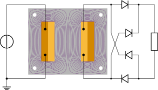
Simulation of devices and their surrounding circuitry is often performed with circuit simulators. Within such simulations, the behaviour of the devices is described by lumped element models, which yield algebraic or differential relations between the voltages and the currents. A disadvantage of the lumped models is that they do not provide enough details, whenever a spatial description of the electromagnetic field inside a device is needed. Such cases include for example the simulation of electric machines [1] or of the quench protection system of superconducting magnets in particle accelerators [2]. In these cases field/circuit coupling [3, 4, 5] is needed, see Fig. 1. In order to exploit the different time rates and also to be able to use separate dedicated solvers for the different systems of equations involved, waveform relaxation (WR) is often used [6]. Here, the different systems of equations are solved separately and, iteratively, information is exchanged between them until they converge to the coupled solution.
For the numerical solution of the field system, space is discretised first e.g. with the finite element method (FEM). Together with the circuit equations this results in systems of differential algebraic equations (DAEs), which have to be solved in the time domain. The finer the mesh, the larger are the systems to be solved at every time step. This leads to long computational time. To this end, calculations can be accelerated by means of a parallel-in-time method called parareal, which is a specific shooting method [7, 8].
This work combines parareal and WR together in one algorithm. In contrast to previous works, e.g. [9, 10], engineering knowledge is used to design a new and optimised algorithm which significantly reduces the computational cost borrowing ideas from micro/macro parareal [11, 12].
The structure of the paper is the following: Section 2 introduces the spatially discretised systems of equations. Section 3 explains the waveform relaxation algorithm with an optimised transmission condition for the field/circuit coupled case. In section 4 the classical as well as a special case of the micro/macro parareal algorithm are introduced. Section 5 deals with the coupling of waveform relaxation and parareal and finally section 6 presents numerical simulations. The last section closes the paper with conclusions and an outlook to the future work.
II Systems of equations
To describe the electromagnetic field part, we consider a magnetoquasistatic approximation of Maxwell’s equations in terms of the reduced A formulation [14]. This leads to the curl-curl eddy current partial differential equation (PDE) that describes the field in terms of a magnetic vector potential. The circuit side is formulated with the modified nodal analysis (MNA) [15]. For the numerical simulation of the coupled system, the method of lines is used. This leads to a time-dependent coupled system of DAEs that are formulated as an initial value problem (IVP).
For we solve the IVP described by the coupled system. The field DAEs are
| (1) | ||||
| (2) |
where is the discretised magnetic vector potential, the voltage across and the current through the coil of the electromagnetic device. denotes the (singular) mass matrix, the (possibly gauged) curl-curl matrix, and distributes the circuit’s input currents in space based on the stranded conductor model. In two dimension, we consider either
if lamination is considered, [16], where are test and weighting functions from an appropriate space defined on the computational domain , the conductivity and the lamination thickness. We assume that the spaces contain boundary and gauging condition (e.g. tree/cotree) if necessary. The circuit is described in terms of the MNA by the system
| (3) | |||
| (4) |
with containing the node potentials and currents through branches with voltage sources and inductors, the voltage across and the current through branches containing the electromagnetic element, and being the MNA system matrices and the incidence matrix of the field element describing its position inside the circuit’s graph. For the coupling, and and given initial values
| (5) |
III Waveform Relaxation
We start the WR algorithm by dividing the simulation time span into time windows of size . At iteration , a Gauss-Seidel scheme is applied to (1)-(4), which allows to solve the field and circuit systems of equations separately and iteratively exchange information between them until the solution converges up to a certain tolerance.
For each time window and WR iteration , the algorithm starts by solving the field system
| (6) | ||||
| (7) | ||||
| (8) |
In the first WR iteration, is computed by (constant) extrapolation of the initial condition . Afterwards, the circuit can be solved independently with
| (9) | |||
| (10) | |||
| (11) |
where the inductance
| (12) |
is used to optimise convergence [4, 5]. Here, denotes the pseudo-inverse, if necessary due to gauging. These steps are repeated until the difference of the solutions between two subsequent iterations is small enough. Once convergence up to a certain tolerance is reached, the solution obtained at time is used as initial condition for the next time window and the iteration scheme can be repeated again. Thus, the WR algorithm is performed sequentially through all time windows.
Considering the field system’s transmission condition (8), the analogous version for the circuit part would be to set
However, instead, (11) is used. This yields an improved exchange of information between the two systems in the context of optimised Schwarz methods [17]. It corresponds to treating the field as an inductor with a correction voltage source. It has been shown that this leads to faster WR convergence [4, 5].
IV Parareal
The parareal algorithm starts with partitioning the interval into (the same) windows of size . We start by summarizing (1)-(5) as the initial-value problem
| (13) |
with and the degrees of freedom (DoF) of the coupled system. Within the parareal framework, one solves
| (14) |
on each subinterval in parallel, starting from an initial value with a given The goal is then to eliminate the mismatch between the values at synchronisation points The parareal iteration reads [7]: for and
| (15) | ||||
Operators and in (15) are a fine and a coarse propagator, respectively. gives an accurate solution (e.g. using small time steps) of (14), starting from initial values and can be calculated in parallel on all . On the other hand, the coarse solution is obtained in a cheaper way (e.g. using large time steps) but sequentially.
IV-A Micro/Macro Parareal
The idea of micro/macro parareal is to consider different models on the levels. On the fine level, the original problem (13) is solved. However, for the coarse one, a reduced IVP
| (16) |
is considered, with and the number of DoFs of the reduced system. This allows to further speed up the computation of the coarse solution by not only saving the cost of the time stepper, but also reducing the size of the system solved. Here, for example, model order reduction techniques can be used [11] to set up the simplified coarse system in (16).
Now, two additional operators have to be defined, in order to exchange the solutions between the models. The restriction operator allows to, given an initial value of (13), obtain a valid initial value for (16). The inverse can be done with the lifting operator , which, given an initial value of the coarse system, computes a valid initial value for the fine one. They are defined consistently, such that
| (17) |
With these operators, the update in (15) is changed to [11]
| (18) |
with fine and coarse solution .
V Parallelised Waveform Relaxation
For the coupling of WR with parareal (PRWR), we consider the WR and the parareal window sizes to be the same . This choice is not necessary, however a natural one. We present two variants of the algorithm.
The initial version of the algorithm is similar to [10]. Here, we choose both the coarse and the fine propagators to be a WR scheme. For the the coarse propagator, the WR scheme will not iterate until convergence, but will stop after a finite (fixed) number of iterations . In contrast to [10], the fine propagator iterates the WR scheme until convergence up to a certain tolerance.
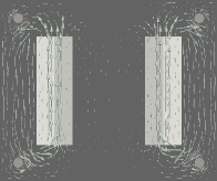
The second algorithm is an optimised version of the first one, where the coarse propagator is chosen to only perform half of a WR iteration () by starting with the circuit system. This means only solving (9)-(11) for and replacing the transformer by a mutual inductor as depicted in Fig. 2 extracted by (12). It can also be interpreted as neglecting the eddy current effects of the magnetoquasistatic problem on the coarse level. This allows to significantly reduce the computational cost as the coarse propagator only operates on the circuit level, i.e. with rather few DoFs. This algorithm fits into the context of micro/macro parareal algorithms [11, 12].

VI Numerical simulations
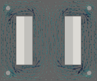
We apply the two introduced approaches to a 2D model of a single-phase isolation transformer (‘MyTransformer’) coupled to a rectifier circuit [4, Fig. 6.6 (b)], which we depict in Fig. 1. For the numerical simulations we consider field-independent materials, such that the eddy-current curl-curl equation (1) is a linear DAE. The simulation interval is chosen as s, which is partitioned into windows. For the time integration inside the WR scheme of both coarse and fine propagators, implicit Euler method is used. The fine time step size is s and the excitation voltage source is V. Parareal is performed until the relative error of the jumps is below .
Firstly the initial algorithm is applied such that the coarse propagator performs WR iterations with time step size for both subsystems. The fine propagator executes WR until convergence (relative error of the coupling variables between two subsequent iterations ).
In the optimised case, the coarse solver only solves the circuit part with a lumped inductance element replacing the field system. This system is solved with a time step size of . For the fine propagator, the solution of the field/circuit coupled problem with WR until convergence (again relative error ) is used. In this case, a micro/macro parareal algorithm arises. Therefore, restriction and lifting operators must be constructed. The DoFs of the fine system are
whereas the coarse operator reduces them to , with
We set the restriction operator to
The lifting computes the corresponding magnetic vector potential obtained from solving a magnetostatic problem with a given current, that is,
Please note that, as stated in (17),
Remark.
In practice, for nonlinear materials, in each parareal iteration and window, the inductance (12) is extracted at a working point and kept constant.
VI-A Simulation results
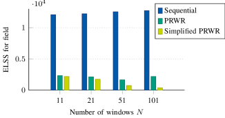
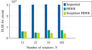
Both algorithms are applied to the same transformer with the eddy current lamination model [16]. The effective number of linear system solves for sequential WR, PRWR with the first algorithm and PRWR with the second algorithm is shown in Fig. 3. It can be seen that, even though both PRWR algorithms significantly decrease the effective number of solutions of linear systems compared to the sequential simulation, the first algorithm is sooner affected by the sequential computation of the coarse system, which increases the effective cost for larger number of processors . The optimised algorithm profits here from the fact that no FEM simulations are necessary on the coarse level.
VII Future work
The simplified algorithm has also been applied to the eddy current problem without lamination of the core. However, the algorithm only converges after the th parareal iteration, which does not yield a speed up with respect to the sequential simulation. This is due to the fact that the eddy current effects are dominant and the static simplification made in the coarse system is not accurate enough. There are two main sources of error arising from the approximation. First, neglecting the eddy current losses leads to a different current to voltage relation on the circuit side. A second source of error is the lifting operator, as it distributes the magnetic vector potential neglecting the skin effect which, for the considered example, is highly relevant. Future work will investigate more sophisticated lumped models and liftings.
VIII Conclusion
This paper proposes a parallel-in-time framework for efficient solution of field/circuit coupled problems. Two approaches of a joint application of the co-simulation technique and parareal are introduced and applied to a single-phase isolation transformer. The results confirm that both approaches converge quickly and allow to reduce the effective computational cost compared to the sequential waveform relaxation simulation. In the best case the time spent on FE computations is sped up by a factor of 33 , i.e. for comparing the field ELSS of Sequential and Simplified PRWR (see Fig. 3).
Acknowledgement
This work is supported by the ‘Excellence Initiative’ of the German Federal and State Governments and the Graduate School of Computational Engineering at TU Darmstadt and DFG Grant SCHO1562/1-2 and BMBF Grant 05M2018RDA (PASIROM). The authors would also like to thank Lorenzo Bortot and Michał Maciejewski for the fruitful discussions.

References
- [1] S. J. Salon, Finite Element Analysis of Electrical Machines. Kluwer, 1995.
- [2] L. Bortot, B. Auchmann, I. Cortes Garcia, A. M. Fernando Navarro, M. Maciejewski, M. Mentink, M. Prioli, E. Ravaioli, S. Schöps, and A. Verweij, “STEAM: A hierarchical co-simulation framework for superconducting accelerator magnet circuits,” IEEE Trans. Appl. Super., vol. 28, no. 3, Apr. 2018.
- [3] G. Bedrosian, “A new method for coupling finite element field solutions with external circuits and kinematics,” IEEE Trans. Magn., vol. 29, no. 2, pp. 1664–1668, 1993.
- [4] S. Schöps, “Multiscale modeling and multirate time-integration of field/circuit coupled problems,” VDI Verlag. Fortschritt-Berichte VDI, Reihe 21, Düsseldorf, Germany, May 2011.
- [5] I. Cortes Garcia, S. Schöps, L. Bortot, M. Maciejewski, M. Prioli, A. M. Fernandez Navarro, B. Auchmann, and A. P. Verweij, “Optimized field/circuit coupling for the simulation of quenches in superconducting magnets,” IEEE J. Multiscale Multiphys. Comput. Tech., vol. 2, no. 1, pp. 97–104, May 2017.
- [6] E. Lelarasmee, A. E. Ruehli, and A. L. Sangiovanni-Vincentelli, “The waveform relaxation method for time-domain analysis of large scale integrated circuits,” IEEE Trans. Comput. Aided. Des. Integrated Circ. Syst., vol. 1, no. 3, pp. 131–145, 1982.
- [7] J.-L. Lions, Y. Maday, and G. Turinici, “A parareal in time discretization of PDEs,” Comptes Rendus de l’Académie des Sciences – Series I – Mathematics, vol. 332, no. 7, pp. 661–668, 2001.
- [8] M. J. Gander, “50 years of time parallel time integration,” in Multiple Shooting and Time Domain Decomposition Methods, ser. Contributions in Mathematical and Computational Sciences, T. Carraro, M. Geiger, S. Körkel, and R. Rannacher, Eds., vol. 9. Springer Berlin Heidelberg, 2015, pp. 69–113.
- [9] J. Liu and Y.-L. Jiang, “A parareal waveform relaxation algorithm for semi-linear parabolic partial differential equations,” J. Comput. Appl. Math., vol. 236, no. 17, pp. 4245–4263, 2012.
- [10] T. Cadeau and F. Magoules, “Coupling the parareal algorithm with the waveform relaxation method for the solution of differential algebraic equations,” in 10th International Symposium on Distributed Computing and Applications to Business, Engineering and Science, Oct. 2011, pp. 15–19.
- [11] Y. Maday, J. Salomon, and G. Turinici, “Monotonic parareal control for quantum systems,” SIAM J. Math. Anal., vol. 45, no. 6, pp. 2468–2482, 2007.
- [12] F. Legoll, T. Lelièvre, and G. Samaey, “A micro-macro parareal algorithm: Application to singularly perturbed ordinary differential equations,” SIAM J. Sci. Comput., vol. 35, no. 4, pp. A1951–A1986, Aug. 2013.
- [13] D. Meeker, Finite Element Method Magnetics, version 4.2 (25feb2018 build) ed., 2018, user’s Manual. [Online]. Available: http://www.femm.info/
- [14] C. R. I. Emson and C. W. Trowbridge, “Transient 3d eddy currents using modified magnetic vector potentials and magnetic scalar potentials,” IEEE Trans. Magn., vol. 24, no. 1, pp. 86–89, Jan. 1988.
- [15] C.-W. Ho, A. E. Ruehli, and P. A. Brennan, “The modified nodal approach to network analysis,” IEEE Trans. Circ. Syst., vol. 22, no. 6, pp. 504–509, Jun. 1975.
- [16] J. Gyselinck, L. Vandevelde, J. Melkebeek, P. Dular, F. Henrotte, and W. Legros, “Calculation of eddy currents and associated losses in electrical steel laminations,” IEEE Trans. Magn., vol. 35, no. 3, pp. 1191–1194, May 1999.
- [17] M. Al-Khaleel, M. J. Gander, and A. E. Ruehli, “Optimization of transmission conditions in waveform relaxation techniques for RC circuits,” SIAM J. Numer. Anal., vol. 52, no. 2, pp. 1076–1101, 2014.