Spacetime Colour Reconnection in Herwig 7

Abstract

We present a model for generating spacetime coordinates in the Monte Carlo event generator Herwig 7, and perform colour reconnection by minimizing a boost-invariant distance measure of the system. We compare the model to a series of soft physics observables. We find reasonable agreement with the data, suggesting that $pp$-collider colour reconnection may be able to be applied in larger systems.

1 Introduction

As the LHC reaches unprecedented levels of precision and data collection, the playground for studying QCD effects has increased manifold. In particular, Monte Carlo event generators Bahr:2008pv ; Bellm:2017bvx ; Herwig7 ; Sjostrand:2014zea ; Gleisberg:2008ta provide an ideal arena for testing novel ideas in the low-energy regime, i.e. the mechanisms of hadronization, where non-perturbative effects have to be phenomenologically modelled, and the underlying event. One aspect of proton-proton collisions that is poorly understood is exactly how multiple parton-parton interactions from the initial scattering process interfere and interact with one another during the hadronization stage.

Multiple parton interactions were first introduced in Sjostrand:1987su , and implemented in Pythia Sjostrand:2014zea , where its importance in hadronic collisions was highlighted beyond a doubt. A similar physical notion was introduced in Butterworth:1996zw and later implemented in Herwig++ Bahr:2008dy ; Bahr:2008pv ; Bahr:2009ek , with some recent improvements to soft and diffractive scatterings in Gieseke:2016fpz ; Bellm:2017bvx to Herwig 7.

One such model of this interference between subcollisions in an event is colour reconnection Sjostrand:1993hi ; Gieseke:2012ft ; Bierlich:2015rha ; Gieseke:2017clv ; Christiansen:2015yqa , whereby a Monte Carlo event generator reduces some kinematic, momentum-based measure of the event. The physical intuition for such a mechanism is twofold: to correct for errors in the leading-colour approximation of the parton shower, and to allow multiple parton interactions, which may have been colour-connected, to have cross-talk. A summary of the history of colour reconnection and the effects of such a mechanism on precise measurements is given in Sjostrand:2013cya . Colour reconnection in Herwig 7 first focused on reconnecting excited $q\bar{q}$ pairs called clusters, minimizing the sum of the invariant masses. Later work Gieseke:2017clv expanded upon this model to introduce the possibility of forming so-called baryonic clusters $qqq$ and $\bar{q}\bar{q}\bar{q}$ from three ordinary/mesonic clusters. Other methods have investigated colour reconnection at the perturbative stages of event simulation or taken inspiration from perturbative techniques Lonnblad:1995yk ; Gieseke:2018gff ; Bellm:2018wwz .

Most $pp$ event generators are developed in the energy-momentum framework for the various stages of event simulation, meaning that none of the physics modelled involves any notion of spacetime separation. While the energy-momentum framework has been very successful, there are still several issues at hand. In particular, it does not have an adequate answer to what parts of the event are allowed to undergo colour reconnection within a given slice of phase space, if one thinks that colour reconnection needs to be a causal effect. Collisions of heavy ions have shown that spacetime structure is important in modelling where interactions start, since a jet starting at the edge of the quark-gluon plasma will lose far less energy to one travelling through the centre of dense medium, a phenomenon known as jet quenching Bjorken:1982tu ; Gyulassy:1990ye ; Qin:2015srf . As a result, $pp$-oriented event generators have also started to include more spacetime information, using these coordinates for various aspects of the simulation, such as collective hadronization effects Bierlich:2014xba ; Bierlich:2016vgw , and a spacetime evolution of the parton shower Ellis:1995fi . Pythia recently introduced a framework for generating spacetime coordinates Ferreres-Sole:2018vgo for quantitative studies of Lund string fragmentation Andersson:1983ia . The effects of introducing spacetime coordinates have been recently studied in dipole evolution in $\gamma^{*}A$ collisions Bierlich:2019wld .

As high energy and heavy ion phenomenology begin to have more interaction with each other, an immediate question one should ask is if the models developed in each field can be applied to the other successfully. Without spacetime information, high energy event generators cannot hope to be able to describe hadronization of large systems well. This work aims to be the first steps of introducing spacetime coordinates and using them to aid the baryonic colour reconnection model Gieseke:2017clv . We intend this to be a proof of concept that will allow us to apply this hadronization model to heavy ions in later work.

The format of the article is as follows: we start by recalling elements of modelling high energy collisions, such as the underlying event, cluster hadronization, and colour reconnection models in Herwig 7, in Sec. 2. In Sec. 3, we describe our method of systematically assigning coordinates to the multiple parton interactions and the partons at the end of the shower. We then present our model of using this spacetime information to perform colour reconnection in Sec. 4. We briefly describe additional modifications that have been applied in the making of this and related works in Sec. 5. We tune our new model in Sec. 6 and present the results of the procedure in Sec. 7. Lastly, with Sec. 8, we summarize our model and future work.

2 Event Simulation in Herwig 7

We briefly summarize the pertinent points of modelling the underlying event and hadronization in Herwig 7.

2.1 Multiple parton interactions (MPI)

Since the proton is a composite particle, when two protons collide, there may be several parton-parton interactions, which fall into two classes in Herwig 7: hard and soft. Partons from hard scatters undergo parton showering, while soft scatters do not.

For a given event, Herwig 7 generates a number of each type of these scatters. The average number of interactions for a given impact parameter $b$ and centre of mass energy $s$ is schematically given by:

$$\langle n_{\mathrm{int}}\rangle=A(b;\mu)\sigma^{\mathrm{inc}}(s;p_{\perp}^{\mathrm{min}}),$$ (1)

where $\sigma^{\mathrm{inc}}$ is the inclusive cross section to produce a pair of partons above a defined minimum transverse momentum, $A(b;\mu)$ is the overlap function between the two protons, and $\mu^{2}$ is commonly referred to as the inverse hadron length. In Herwig 7, both the hard and soft MPI scatters have the same form for Eq. 1, and indeed it is assumed that they both have the same functional form for the overlap function, but with different values for $\mu^{2}$. Similarly, the inclusive cross sections are different values for hard and soft scatters.

Herwig 7 assumes the MPI to be independent of one another (including energy-momentum conservation), leading to a Poissonian probability distribution. Using the notation of Herwig7 , we can write the joint probability distribution to produce $h$ hard and $k$ soft scatters at a given b as:

$$\mathcal{P}_{h,k}(b)=\frac{\left(2\chi_{h}\right)^{h}}{h!}\frac{\left(2\chi_{k}\right)^{k}}{k!}e^{-2(\chi_{h}+\chi_{k})},$$ (2)

where $2\chi_{h,k}=A(b;\mu_{h,k})\sigma^{\mathrm{inc}}_{h,k}$ is the so-called eikonal factor. This formalism was developed in Aurenche:1991pk and Herwig’s implementation is built on the JIMMY framework Butterworth:1996zw .

Eq. 2 is then integrated over $b$ space to produce an exact probability to produce the corresponding number of hard and soft scatters in an event:

$$P_{h,k}=\frac{\int\text{d}^{2}b\mathcal{P}_{h,k}(b,s)}{\int\text{d}^{2}b\sum_{h\geq 1,k=0}^{\infty}\mathcal{P}_{h,k}(b,s)}.$$ (3)

Herwig 7 samples the distribution in Eq. 3 probabilistically, to obtain a number $h$ of hard scatters, and $k$ of soft scatters. The primary hard subprocess in Minimum Bias event generation in Herwig 7 is an interaction between two valence (antiquarks) Gieseke:2012ft , while subsequent MPI collisions are initiated by regular $2\to 2$ QCD processes. The incoming legs are evolved backwards to pairs of gluons extracted from the beam remnant, with the colour topology defined in the $N_{C}\to\infty$ limit. The colour topology is motivated by the leading-colour approximation used in the shower, though as discussed in Gieseke:2012ft , this is a phenomenological choice rather than an approximation.

As Herwig 7 produces each scatter, it checks the available energy and momentum in the protons. If the protons cannot produce another scatter, the MPI production algorithm terminates. As a result, Herwig 7 typically generates a subset of the total number of scatters sampled from Eq. 3. More details of the technicalities involved in the implementation of MPI algorithm can be found in Bahr:2008pv .

2.2 Cluster model

Partons from a scattering process are showered down to the parton shower cutoff scale, and the resulting colour topology has triplets connected to anti-triplets via gluon connections. At the hadronization scale and below, Herwig 7 uses the cluster hadronization model WEBBER1984492 , based on the pre-confinement property of angular-ordered showers AMATI197987 .

The first step in the cluster model is to non-perturbatively split the gluons into quark-antiquark pairs. To split the gluons, Herwig 7 uses a kinematic map at the end of the shower to put the gluons on-constituent-mass-shell and performs an isotropic decay. The constituent-mass of the gluon is a non-perturbative parameter of Herwig 7 hadronization model.

Nearest quark-antiquark neighbours in colour space, which are typically nearest neighbours in momentum space due to pre-confinement, are then collected into colourless, excited quark-antiquark pairs, i.e. clusters. From there, the clusters undergo colour reconnection.

2.3 Colour reconnection

Clusters typically connect partons from the same multiple parton interaction scattering. Colour reconnection alters the colour topology of the event, and allows the different MPI to interact with one another at the hadronization level.

As mentioned in Sec. 2.1, Herwig 7 chooses the leading-colour topology for the additional scatters, thus they are colour-connected to the beam remnant and other subprocesses. As noted in Gieseke:2012ft , colour reconnection is a required part of hadronization modelling in hadron collisions since the leading-colour approximation performs significantly worse in non-perturbative parts of the event generation.

Colour reconnection aims to minimize a given measure of the event, typically momentum-based. Herwig 7 has a variety of colour reconnection algorithms Gieseke:2012ft ; Gieseke:2017clv , namely:

• Plain,

• Statistical/Metropolis,

• Baryonic.

The plain colour reconnection model locally minimizes pair-wise cluster invariant masses:

$$m_{q\bar{q}}^{2}=\left(p_{q}+p_{\bar{q}}\right)^{2}.$$ (4)

The criteria for two clusters to undergo colour reconnection and swap partners is:

$$m_{q\bar{q}^{\prime}}+m_{q^{\prime}\bar{q}}<m_{q\bar{q}}+m_{q^{\prime}\bar{q}^{\prime}}.$$ (5)

If a pairing reduces the invariant mass, it is allowed to reconnect with a flat probabilistic weight, typically tuned to LHC data, while ensuring that the model doesn’t adversely affect LEP simulations. Baryonic colour reconnection was recently implemented in Herwig 7 Gieseke:2017clv , and it uses a more sophisticated algorithm. For each cluster in the event, the algorithm searches for other clusters which occupy the same neighbourhood in rapidity-space. It searches for two types of candidate clusters for reconnection: baryonic, and (ordinary) mesonic.

In the baryonic case, given a cluster A, transform the momenta of all other clusters to the rest frame of A, and search for two other clusters that have the same orientation of quark axis in rapidity space. It then chooses the pair of candidate clusters which have the largest rapidity span in this frame. If the reconnection is accepted, the quarks are then collected into a three-component cluster, called a baryonic cluster, and similarly the antiquarks are collected into an anti-baryonic cluster.

In the mesonic case, if the candidate cluster B with the largest rapidity span has a quark axis oriented in the opposite direction to cluster A, reconnect $q_{A}\bar{q}_{B}$ and $q_{B}\bar{q}_{A}$, in much the same manner as the plain colour reconnection model. For both types of cases in baryonic colour reconnection, the probabilities for reconnection are given by two different flat weights, $p_{\text{M,reco}}$ and $p_{\text{B,reco}}$.

While the statistical colour reconnection model is outside the scope of this paper, we mention that it aims to minimize mass, much like the plain model, but it allows reconnection to increase the mass of the system with a suppressed probability, and is based on the simulated annealing optimization algorithm Kirkpatrick671 .

In all cases, colour reconnection qualitatively aligns colours between partons that move into the same direction such that the multiplicity of particles produced in between them is reduced and the produced particles carry more momentum on average.

3 Spacetime Coordinate Generation

We present the two parts of how our model systematically generates coordinates for the multiple parton interaction scattering centres and the hadronization stage. We argue that these are the two stages of event generation that are most impactful on spacetime coordinates.

3.1 MPI coordinate generation algorithm

To obtain an intelligent and relevant value for the impact parameter, the MPI coordinate generator takes the produced values for $h,k$ in Eq. 3 and stochastically samples the distribution of Eq. 2, vis-a-vis a veto algorithm. Thus, the produced $b$, when the number of events tends to infinity, will be the correct distribution for a given set of $h$ and $k$.

As shown in Fig. 1, the joint Poissonian behaves as we expect. The more scatters that Herwig 7 produces, the more likely it is that the sampled $b$ will be central, while having more soft scatters for a fixed number of total scatters makes the distribution have a broader tail. In this work we will be using the Bessel proton profile, meaning that the overlap function is a Bessel function of the third kind:

$$A(b;\mu)=\frac{\mu^{2}}{96\pi}(\mu b)^{3}K_{3}(\mu b).$$ (6)

It should be noted that the results of the sampling should not be surprising. At large numbers of interactions, the sampled impact parameters tend to be closer to 0, since a larger than average number of interactions requires a more central collision. Once $b$ is determined for a given event, we set the incoming beam positions to be at $(\pm b/2,0,0,0)$, i.e. aligned along the $x$-axis, for simplicity.

The overlap function $A(b;\mu)$ in Eq. 6 is generated by the convolution of the two protons’ form factors, $G(b;\mu)$:

$$A(b)=\int\mathrm{d}^{2}b^{\prime}G(b^{\prime})G(b-b^{\prime}),$$ (7)

where we have suppressed the dependence on $\mu$ for clarity. The overlap function governs the density of MPI scattering centres in the transverse plane for a given offset between the protons.

To obtain the MPI centre positions, we sample the integrand of Eq. 7. We generate $h$ hard scatters, and $k$ soft scatters, using two different $\mu^{2}$ values for the hard and soft interactions. As a result, hard scatters are slightly more concentrated in the centre of the transverse plane, while soft scatters have a longer tail.

Once these points have been generated, all coordinates including the proton positions get the same random global rotation in the transverse plane. The beam remnants receive the sampled proton positions. A schematic diagram of the results of the MPI coordinate generation algorithm is shown in Fig. 2. The overlap need not necessarily be a Bessel function, and we have included the results of the MPI coordinate generation for a uniform proton profile in Fig. 2. For this type of proton profile, MPI centres can only be situated in the overlap. However, for the rest of the paper, we will work with the Bessel function profile.

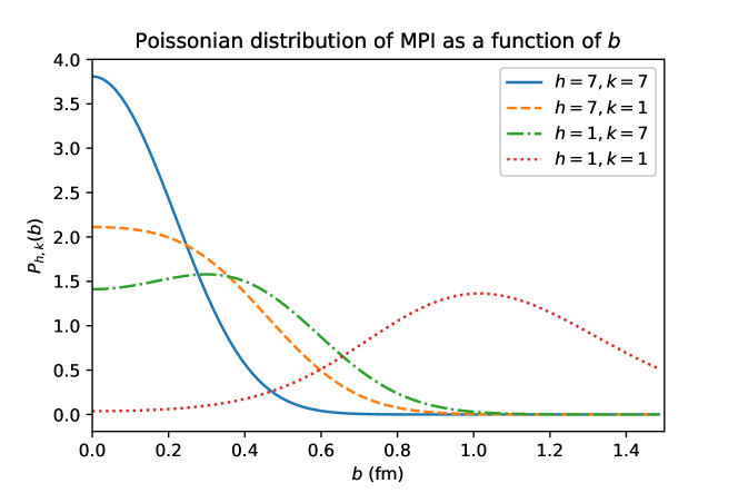
Figure 1: Joint Poissonian distribution $\mathcal{P}_{h,k}(b)$, as a function of impact parameter $b$, for a number of $h$ hard scatters and $k$ soft scatters. We have picked one large (7) and one small (1) value, and show the various combinations. The more collisions that occur, the more likely the collision is to be central. Keeping the number of interactions fixed but having more soft interactions makes the distribution have a broader tail. We have used the following fixed values for the normalized distributions: $\sigma^{\mathrm{inc}}_{\mathrm{hard}}=83~{}\mathrm{mb}$, $\sigma^{\mathrm{inc}}_{\mathrm{soft}}=127~{}\mathrm{mb}$, $\mu^{2}_{\mathrm{hard}}=0.71~{}\mathrm{GeV}^{2}$, and $\mu^{2}_{\mathrm{soft}}=0.52~{}\mathrm{GeV}^{2}$. These distributions are normalized independently to unit area.

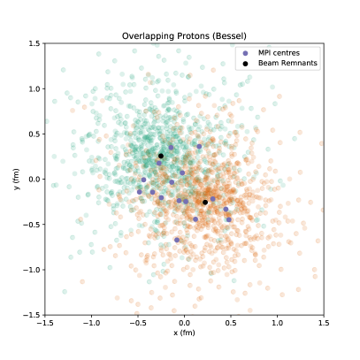
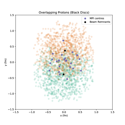
Figure 2: Result of MPI Coordinate Generator algorithm with the Bessel proton profile (left), and an example for a uniform (black disc) proton profile (right). Green and orange points are partons sampled in a given proton, mauve points are accepted MPI collision centres, and black are the beam remnants.

3.2 Tracing spacetime during parton showers

The spacetime structure of the parton-shower evolution was already considered in the early paper on QCD cascades by Fox and Wolfram (see Fig. 1 of Fox:1979ag ). Later the spacetime evolution of the parton shower was introduced, for example, to study jets in hadronic $e^{+}e^{-}$ events at LEP Ellis:1995dq and in deep-inelastic ep scattering Ellis:1996nv . Very recently in a publication on the space–time structure of hadronization in the Lund Model Ferreres-Sole:2018vgo the authors mention that a sensible spacetime picture of parton-shower evolution would introduce some spacetime offsets to their model. However, the authors assumed that the offsets are most likely small in their case and therefore neglected them in their studies.

In the following section, we will investigate in more detail how the parton shower affects the spacetime structure of an event as implemented in the family of Herwig 7 generators. Referring to Corcella:2000bw (Section 3.8) for details, we briefly recall the essential concepts of the Herwig 7 spacetime model. It should be noted that there are two major parton shower options in Herwig, namely the angular-ordered shower Gieseke:2003rz and the dipole shower Platzer:2009jq . For this work, we will focus on the angular-ordered shower, and its use of virtuality as an evolution variable.

The mean lifetime $\tau$ of a parton in its own rest frame, during the parton shower evolution, is calculated in a similar manner as for particles decays, i.e. taking into account its natural width $\Gamma$ and virtuality $q^{2}$:

$$\tau(q^{2})=\frac{\hbar\sqrt{q^{2}}}{\sqrt{\left(q^{2}-M^{2}\right)^{2}+\left(\frac{\Gamma q^{2}}{M}\right)^{2}}},$$ (8)

Eq. 8 interpolates between the lifetime for an on-mass shell parton $\tau(q^{2}=M^{2})=\hbar/\Gamma$, and for a highly virtual (i.e. off-mass shell) parton $\tau(q^{2}\gg M^{2})=\hbar/\sqrt{q^{2}}$. We note that the mean lifetime in Eq. 8 is equivalent to the standard notion of formation time used in heavy ion phenomenology as well as in general jet quenching research Baier:2000mf ; Casalderrey-Solana2016 ; Blaizot:2019muz ; Dominguez:2019ges . We show the equivalence in App. A.

Once a lifetime is calculated according to Eq. 8, the parton decays according to an exponential decay law, with a rest-frame decay time $t^{*}$:

$$P_{\text{decay}}(t<t^{*})=1-\exp\left(-\frac{t^{*}}{\tau}\right).$$ (9)

After sampling a rest-frame decay time, this time can be converted to the lab-frame decay time $t$, and a distance travelled in the lab-frame, $\vec{d}$:

$$t=\gamma t^{*},\vec{d}=\vec{\beta}\gamma t^{*},$$ (10)

where $\gamma$ and $\vec{\beta}$ are the usual Lorentz factors.

Very light quarks and gluons with a small natural width may travel unphysically large distances according to Eq. 8 in the final steps of the parton shower. Similarly, there are issues with assigning particles with no well-defined width spacetime coordinates in the above manner. In order to counter this issue, a minimum width $\Gamma=\nu^{2}/M$ is introduced, where $\nu^{2}$ (GeV²) is a free parameter of the order of lower limit of parton’s virtuality. This is essentially the spacetime equivalent of a shower $Q^{2}\approx\Lambda_{\mathrm{QCD}}^{2}$ cutoff scale. The daughters of the parton splitting are then given the starting coordinates defined by Eq. 10. We note that the above considerations are, in our model, a phenomenological model of the spacetime structure of an event, which arise during the initial collision of the protons, and the subsequent perturbative evolution of the event.

In order to study the size of the parton-shower spacetime effects, we will first consider the distance that each parton propagates during the shower. The distance that we are interested in is the difference between a given parton’s production and decay vertex, $L$:

$$L=\sqrt{\left(d_{\rm decay}-d_{\rm prod}\right)^{2}},$$ (11)

where $d\equiv d^{\mu}=(t,x,y,z)$ is the position of a parton relative to the centre of the collision, i.e. the origin. However, since the MPI smearing discussed in the previous section affects only the transverse plane we will also consider transverse distance, constructed from the transverse components of the above vertices, $r=\sqrt{\Delta x^{2}+\Delta y^{2}}$.

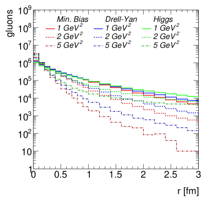
Figure 3: The total Lorentz-invariant distance $L$ (left panel) and transverse distance $r$ (right panel) traveled by the gluons at the last step of the parton shower evolution for three different processes: Minimum Bias, Drell-Yan and Higgs-boson production at the LHC at the centre-of-mass energy $7$ TeV. The simulation was performed using default version of Herwig 7 using three different values of $\nu^{2}$: $1$, $2$ and $5$ GeV².

In Fig. 3 we show the Lorentz-invariant distance $L$ (left panel) and transverse distance (right panel) traveled by the gluons at the last step of the parton shower evolution for three different processes: Minimum Bias, Drell-Yan and Higgs-boson production at the LHC at the collision energy $7$ TeV. The simulation was performed using default version of Herwig 7 with three different values of $\nu^{2}$: $1$, $2$ and $5$ GeV². We see that most of the partons reach fermi-scale distances which are comparable to the size of the MPI coordinate generation, as shown in Fig. 2. Therefore, it is important to take the parton shower effects into account. We also see that in soft Minimum Bias processes the partons travel shorter distances, as expected since there is less parton-shower activity in these types of events than in the two other processes. Finally we see that the results, and especially the long distance tails of the distributions, are strongly dependent on the scale $\nu^{2}$. This indicates that the furthest distances are traveled by partons in the final step of the evolution.

This is also visible in Fig. 4 where we show the spacetime structure of a parton shower of a sample Minimum Bias event, with $\nu^{2}=1$ GeV², neglecting the spacetime structure of the MPI positions. The final step distances are denoted by red dotted lines, while the intermediate steps are black solid lines. In order to quantify this effect in Fig. 5 we show the ratio of distance traveled by partons in the last step of their evolution to the total distance (distance traveled during the entire evolution).

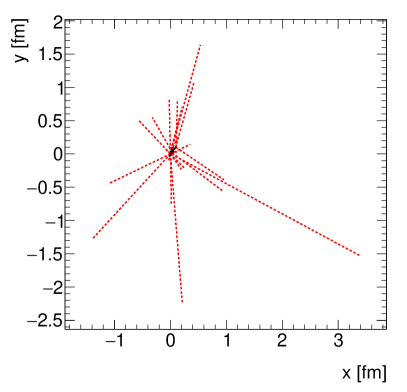
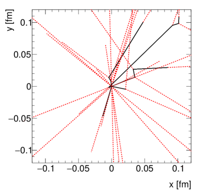
Figure 4: An example of a parton shower spacetime structure (i.e. neglecting spacetime structure of MPI) of a Minimum Bias event in the transverse plane generated with the minimum virtuality $\nu^{2}=1$ GeV². The red dotted lines represent the evolution of the last particle in the parton shower while the rest of the evolution is denoted by the black lines. Both panels show the same event with the right panel magnifying the center of the event.

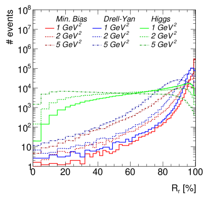
Figure 5: The ratio of the distance traveled by partons in the last step of evolution to the total distance (distance traveled during entire evolution).

We see that in the case of both Minimum Bias and Drell-Yan processes for $\nu^{2}$ values similar to a typical parton-shower cutoff scale, i.e. below $2$ GeV², 90% of the total distance is indeed due to the final step of the parton shower. In the case of the Higgs boson production, the distributions look very different. It is because in the simulation we took into account the decay lifetime of the Higgs boson, however when we neglect it, the distributions look very similar to the two other processes.

To summarize, we can expect the fermi-scale parton shower and even further intermediate particle decay distances. As such, these effects have to be included in spacetime colour reconnection model. We also showed that tracing out the microscopic detail of the parton shower spacetime evolution is somewhat unnecessary, since only the low-energy scale of emissions (final steps) have any major impact on the spacetime position of partons, i.e. soft emissions close to the hadronization scale. Finally, it is important to stress that the Heisenberg uncertainty relations impose limits on how much simultaneous energy–momentum and spacetime information one can have on an individual parton.

These results should not be considered as physical, but give us a benchmark of roughly what part of the event simulation drives the creation of large separations in distance between partons.

Instead, we propose a simpler model that assigns coordinates only to the very last partons of the parton shower, just before the hadronization. This is in line with the uncertainty principle as the smearing is only visible for particles at a very soft scale. We may understand the partons’ positions then as being smeared out around the scattering centres. This idea represents us taking the semi-classical limit of the parton shower, and generating coordinates in a similarly semi-classical manner.

3.3 Parton shower coordinates

As the partons propagate during the shower, we may assign a spacetime propagation to their motion, but as we have shown above, these distances are only significant at energy levels close to the hadronization scale. As a consequence, we will only give spacetime coordinates to the partons that remain at the end of the shower. In our model of spacetime coordinates, we will not consider $z,t$ coordinates and keep our discussion to the transverse plane. We note that we have chosen the centre of mass frame in order to construct our model, and to extend this to any given frame, one need only transform the variables correspondingly. All considerations below will be invariant to any boosts along the $z$-axis.

Before the clusters are formed, each surviving parton from a given MPI scattering centre receives an extra transverse propagation distance from the scattering centre coordinates. Instead of tracing out the positional history of each parton during the shower, we take all partons at the end of the shower and propagate them according to Eq. 9. As argued above, this resembles a smearing of each partons’ coordinate around the scattering centre within its intrinsic uncertainty.

As discussed in Sec. 3.2, at the end of the perturbative shower, partons will have very small virtualities, meaning that using the precise form of Eq. 8 performs poorly. We instead approximate the mean lifetime by considering the width term in the denominator. Each parton of species $p$ will automatically receive a minimum virtuality, $\nu^{2}$, for their mean lifetime in their rest-frame:

$$\tau_{0,p}=\frac{\hbar m_{p}}{\nu^{2}}.$$ (12)

This mean lifetime is derived from Eq. 8, by taking the on-mass shell limit - $\tau(q^{2}=M^{2})=\hbar/\Gamma$ and using the following form for the width of the on-mass shell partons:

$$\Gamma=\frac{\nu^{2}}{m_{p}}.$$ (13)

With the mean lifetime from Eq. 12, we proceed as explained in Sec. 3.2, using Eqs. 9 and 10 to set each parton’s position relative to the MPI scattering centre that they originated from, adding only the transverse coordinates of the propagation distance.

Eq. 12 corresponds to a lab-frame mean lifetime of:

$$\tau^{\prime}_{0,p}=\gamma\tau_{0,p}=\frac{\hbar E_{p}}{\nu^{2}},$$ (14)

where $E_{p}$ is the lab-frame energy of the given parton. The main motivation for the mass dependence of the mean lifetime in Eq. (12) is that the decay distance of external light quarks is proportional to their energy (and independent of their mass) which is in agreement with expectations from the linear confining potential of QCD, see e.g. Bali:2000un and references therein, as well as other hadronization models such as the Lund string model Andersson:1983ia .

As a result of this construction, quark-antiquark pairs produced during the non-perturbative gluon splitting will receive the same spacetime position. One may believe this leads to issues where colour reconnection wants to pair these partons together, but Herwig 7 does not allow them to since they would be in a colour-octet state Gieseke:2012ft ; Reichelt:2017hts . These partons will also have slightly different rapidities, due to kinematics from the gluon splitting.

Once all the partons have their new coordinates with respect to their MPI scattering centre, we then shift these coordinates using the points produced from the MPI coordinate generator, as shown schematically in Fig. 6. The black points are the MPI centres, and partons from those systems are spread by Eq. 10, around their respective centre. Different coloured partons refer to partons originating from different MPI systems.

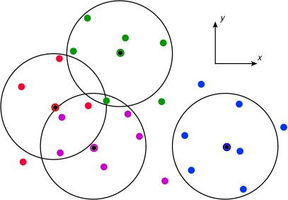
Figure 6: A schematic diagram for how our model introduces transverse spacetime coordinates for the multiple parton interactions (black points), and for the end of the parton shower. Different coloured points are partons from different, respectively ring-coloured MPI centres. The thin black circles represent a characteristic scale for parton propagation about the MPI centre.

4 Spacetime Colour Reconnection

With the transverse coordinates in place, we use this information to perform and inform colour reconnection. We present the outline for plain spacetime colour reconnection model, but we will use the baryonic spacetime model for tuning and in the discussion in the rest of the paper.

4.1 Plain spacetime colour reconnection

As mentioned in Sec. 2.3, the measure for allowing plain colour reconnection is the sum of invariant cluster masses before and after, and the reconnection is given by a flat tuned weight. However, there is at least one major issue with this construction: this measure aims to reconnect cluster constituents so that they are closer in momentum space, but without any input from spacetime which would perhaps prohibit a causally-disconnected colour reconnection.

Using the coordinates we have introduced in Sec. 3, we now define the following spacetime-inspired measure for a single cluster with constituents $i,j$:

$$R_{ij}^{2}=\frac{\Delta r_{ij}^{2}}{d_{0}^{2}}+\Delta y_{ij}^{2},$$ (15)

where $d_{0}$ is the characteristic length scale for colour reconnection in our spacetime model, which is a tunable parameter. $\Delta r_{ij}^{2}=(\vec{x}_{\perp,i}-\vec{x}_{\perp,j})^{2}$ is the transverse spacetime separation squared between the constituent quarks. We include rapidity differences in Eq. 15. This is inspired by conventional jet algorithms, where we replace the azimuthal separation $\Delta\phi_{ij}^{2}$ with transverse separation. The parameter $d_{0}$ effectively acts as a measure to increase the importance of transverse to longitudinal components. The measure in Eq. 15 captures the transverse separation between the constituents and their longitudinal separation.

Using the measure from Eq. 15, we proceed in the same fashion as Eq. 5, by minimizing the sum of the pairing of cluster constituents. For a given cluster, we pick the candidate cluster that minimizes the measure the most. If the sum of the cluster separations is smaller after a possible reconnection:

$$R_{q\bar{q}^{\prime}}+R_{q^{\prime}\bar{q}}<R_{q\bar{q}}+R_{q^{\prime}\bar{q}^{\prime}},$$ (16)

then we accept the reconnection with a flat probability, $p_{\mathrm{M,reco}}$. A similar model was studied earlier in Rohrdiploma .

4.2 Baryonic spacetime colour reconnection

Baryonic spacetime colour reconnection uses the algorithm from Gieseke:2017clv , and outlined in Sec. 2.3. The partners for mesonic and baryonic colour reconnection are found by using the projection onto a given cluster’s quark axis.

If instead we find a baryonic reconnection, we cannot directly compare the sum of Eq. 15 for the constituents of the clusters before and after colour reconnection, since we would be starting with 3 clusters - each with 2 partons - and ending with 2 clusters with 3 partons, and the distance measure is an ill-defined quantity in the latter situation.

In the ordinary baryonic colour reconnection algorithm, 3-component clusters, once formed, are reduced to a quark-diquark system, where the diquark system is chosen as the pair of quarks with the lowest total invariant mass. In keeping with our spacetime paradigm, we choose the pair as the closest in spacetime. Given 3 mesonic clusters, we look at the set of triplets $\{q_{1},q_{2},q_{3}\}$ and select the pair that are closest - calculated via Eq. 15, and similarly for the set of antitriplets. We choose these partons to become a diquark system, with their constituents’ mean spacetime position and rapidity.

We allow baryonic reconnection if the following criterion is true:

$$R_{q,qq}+R_{\bar{q},\bar{q}\bar{q}}<R_{q,\bar{q}}+R_{qq,\bar{q}\bar{q}},$$ (17)

which is analogous to Eq. 16, and we accept this reconnection with probability $p_{\mathrm{B,reco}}=w_{b}$. If the reconnection is rejected, all three candidate clusters remain ordinary mesonic clusters.

We note that the baryonic spacetime colour reconnection has a bias for using rapidity as its first discriminating factor when searching for potential partners. However, we hope that, by using the extra information provided by the transverse separation between constituents, we will be able to improve upon the original baryonic colour reconnection model, especially in larger systems like heavy ion collisions.

To see the spacetime picture of an event, we have produced Fig. 7, which highlights the spacetime coordinate generation procedure outlined in Sec. 3. In the upper panel of Fig. 7, we have plotted all the clusters formed from the non-perturbative gluon splitting at the end of the shower, before any colour reconnection. The points in the plots represent cluster constituents, and the connecting lines represent the clusters.

Performing baryonic spacetime colour reconnection, using $\nu^{2}=1$ GeV², $d_{0}=0.5$ fm, and $w_{b}=0.5$, on this event then produces the lower panel in Fig. 7, where we have highlighted the different types of clusters. Red lines correspond to rearranged clusters: (dotted) baryonic, and (solid) mesonic, while black lines are untouched clusters.

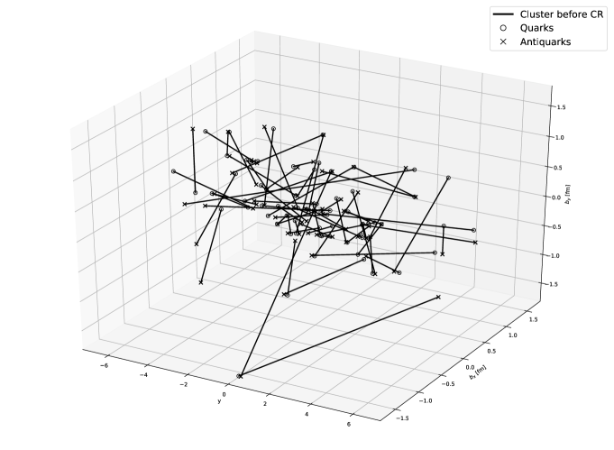
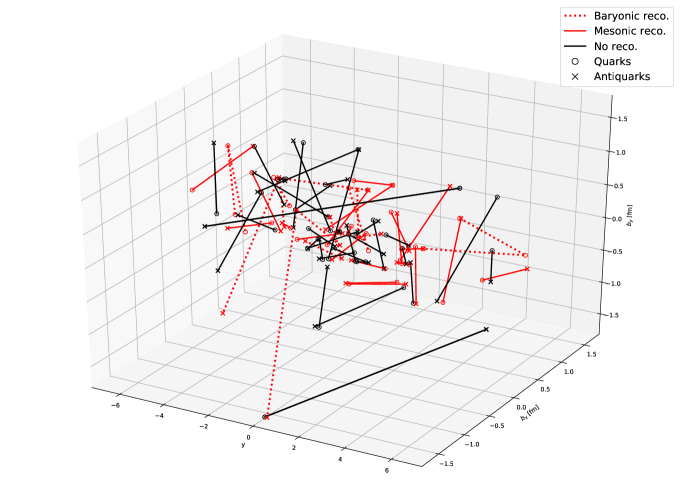
Figure 7: The colour-topology of a sample Minimum Bias event in rapidity and transverse spacetime coordinates, before (top) and after (bottom) colour reconnection. The parameters used for reconnection here are $\nu^{2}=1$ GeV², $d_{0}=0.5$ fm, and baryonic reconnection weight $w_{b}=0.5$. Black lines correspond to clusters which are automatically produced from the parton shower and which have not undergone any colour reconnection, while red lines are the newly rearranged (dotted lines) baryonic and (solid lines) mesonic clusters.

5 Modifications to the Existing Model

While incorporating spacetime coordinates into the Herwig 7 MPI model, we have had to modify parts of the original implementation. These changes are of a more general nature than the specifics of our model. As we wish to focus on the changes that our model has, we will report the changes in a separate contribution Bellm:2019icn . We summarize the most relevant modifications below:

• The kinematics is improved and produces the wanted inclusive spectrum.

• Introduction of diffraction ratio $R_{\mathrm{Diff}}$ parameter for better tuning performance.

• Cross-section handling takes into account the diffractive cross section to calculate the eikonalised cross sections.

• The dummy process used by Herwig 7 in Minimum Bias events is replaced to contain only initial state quarks.

• The partner finding process and scale setting are modified with respect to the standard Herwig 7 mode.

The effects of these changes and their discussion are postponed to Bellm:2019icn .

6 Tuning

We started the tuning process within the Autotunes Bellm:2019owc framework that internally makes use of the Rivet and Professor frameworks Buckley:2010ar ; Buckley:2009bj for Monte Carlo event generators. To elucidate the effects of parameter variations, we illustrate the modifications in $\chi^{2}$-values in Fig. 8. Here, we show by variation of strongly correlated parameter pairs where the minimum of the parameters are located. The white spaces in the planes for the parameter sets ($R_{\mathrm{Diff}}$, $\sigma_{\mathrm{tot}}$) and ($\mu^{2}_{\mathrm{hard}}$, $p_{\perp}^{\mathrm{min}}$) are regions in parameter space where the model fails to fit the soft and hard cross-sections without violating the total cross-section. In the left $\chi^{2}$-plane, we added lines to mark the total cross sections that are predicted by the Donnachie and Landshoff model, where DLMode 1 refers to Donnachie:1992ny , DLMode2 refers to Donnachie:1992ny but normalized to Abe:1993xy .

In the ($\nu^{2}$, $d_{0}$)-plane, we define three parameter points to be used in the later data comparisons. The red point, corresponding to the best fit value ($\nu^{2}=4.5$ GeV², $d_{0}=0.15$ fm) will be referred to as “H7 + STCR”. To show variations in the spacetime model, we choose two other points: blue - ($\nu^{2}=2.1$ GeV², $d_{0}=0.55$ fm), and green - ($\nu^{2}=3.3$ GeV², $d_{0}=0.05$ fm). These two points will be referred to as “Variation 1” and “Variation 2” in the following.

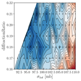
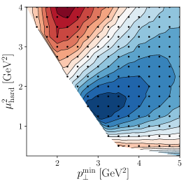
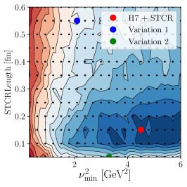
Figure 8: $\chi^{2}$-planes for parameter sets ($R_{\mathrm{Diff}}$, $\sigma_{\mathrm{tot}}$), ($\mu^{2}_{\mathrm{hard}}$, $p_{\perp}^{\mathrm{min}}$) and ($\nu^{2}$, $d_{0}$). Bluer areas in the $\chi^{2}$ contour plots correspond to smaller $\chi^{2}$ values. In the right plot we pick three parameter pairs to define variations to be shown in the data comparison, see Figs. 9 to 12.

We compared the model in the tuning procedure to data from Adam:2015qaa ; Abelev:2012sea ; Aad:2010ac ; Aad:2010fh ; Khachatryan:2015gka and the red parameter point in Fig. 8 corresponds to the parameters that are reflected in Tab. 1.

$\sigma_{\mathrm{tot}}~{}[\mathrm{mb}]$	$R_{\mathrm{Diff}}$	$p^{\mathrm{min}}_{\perp}~{}[\mathrm{GeV}]$	$\mu^{2}_{\mathrm{hard}}~{}[\mathrm{GeV}^{2}]$
$96.0$	$0.2$	$3.0$	$1.5$
$\nu^{2}~{}[\mathrm{GeV}^{2}]$	$d_{0}~{}[\mathrm{fm}]$	$w_{b}$	($\mu^{2}_{\mathrm{soft}}~{}[GeV^{2}]$)
$4.5$	$0.15$	$0.98$	$0.254$

Table 1: The newly tuned parameters for Minimum Bias simulation and our baryonic spacetime colour reconnection model. The top row is the re-tuned parameters of the old Herwig 7 Minimum Bias model. The bottom row is the three new parameters of the spacetime components of our model, and a determined parameter of the old model.

The parameters in the first row have been previously included in the Herwig 7 Minimum Bias model. $R_{\mathrm{Diff}}$ was not explicitly part of the regular model in Herwig 7 but was effectively tuned as the amplitude of the non-diffractive cross section. $p^{\mathrm{min}}_{\perp}$ is the cut on the transverse momentum where the hard MPI component, described by perturbative QCD $2\to 2$ process is taken over by the soft, multi-peripheral MPI model Bahr:2009ek ; Gieseke:2016fpz . The parameter for the inverse proton radius is $\mu^{2}_{\mathrm{hard}}$ and is communicated together with the determined (not tuned) parameter for the soft inverse radius $\mu^{2}_{\mathrm{soft}}$ to the MPI coordinate generator.

The parameters in the second row are the three new parameters introduced for our spacetime model. First, the minimum virtuality $\nu^{2}$, which dictates the traveling of the final partons after the shower step, takes a rather large value $4.5$ GeV² in comparison to the parton shower $Q^{2}$ cutoff.

Second, the colour reconnection distance scale $d_{0}$ in Eq. 15 has a tuned value of 0.15 fm. This length scale is the strength of the transverse component of the spacetime measure relative to the rapidity component. It can also be considered the characteristic length scale of colour reconnection in the transverse plane in our model.

Finally, the baryonic colour reconnection probability weight $w_{b}$, after tuning, has a value of 0.98. This seems to be very large but the model, as described in Gieseke:2017clv , already makes strong restrictions on the possible cluster configurations such that the cluster triplets that are potential candidates for the baryonic reconnection are strongly favoured.

We have kept the probability for strangeness production during the non-perturbative gluon splitting as the tuned value from Gieseke:2017clv , although there have been recent developments in the description of non-perturbative strangeness production in cluster hadronization Duncan:2018gfk . We leave a full retune of all the hadronization parameters to future work.

7 Results

In this section, we describe the data comparison of the tuned parameter set. In Fig. 9, we have collated various cuts on the track momentum, and similarly on the minimum number of charged particles for the rapidity and transverse momentum distributions as measured in Aad:2010ac . Beside the central parameter set (red), we also show the results of the variations as gray lines (solid and dashed). These are crucial observables for the description of Minimum Bias and soft physics, and we find that the model is perfectly capable at describing the distributions.

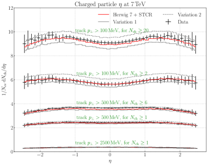
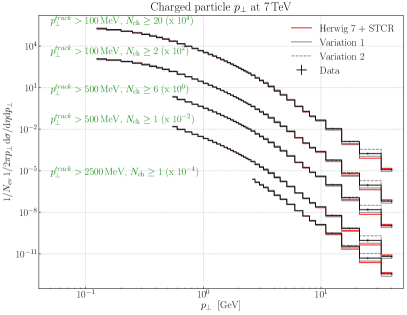
Figure 9: Charged particle spectrum against rapidity and transverse momentum for various leading track $p_{\perp}$ and number of charged particle $N_{\mathrm{ch}}$ slices. An overall good agreement with data is found. The variation is purely in the spacetime length and minimum virtuality parameters of our model as defined in Fig. 8 and in the corresponding text.

In Fig. 10, we compare the differential cross-section with respect to the number of charged particles as measured by Aad:2010ac with our model’s results. We observe that for high charged particle multiplicity the central line overshoots the data and that “Variation 1” is closer to the central data line. With the increased $d_{0}$ in “Variation 1”, the colour reconnection probability is increased. For a high number of additional scatters, the probability is increased to produce smaller clusters and therefore less particle production in the cluster fission and decay processes.

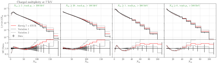
Figure 10: Differential cross-section with respect to the number of charged particles as measured by Aad:2010ac .

To illustrate examples of observables that are hardly modified by the variations in the spacetime components of the model, we show in Fig. 11 the measured rapidity gap fraction and the pion, kaon, and proton yields as measured by Aad:2012pw and Adam:2015qaa . Variations in the spacetime components of the model have very little impact on these observables. The rapidity gap for small values is mostly driven by the hard and soft MPI that could potentially be modified but is known to be relatively invariant to colour reconnection effects. The tail of the rapidity gap cross section is mainly filled by double and single diffraction, which are not modified by the smearing of the MPI collision centers. The fairly poorly described proton yield will be the subject of further studies.

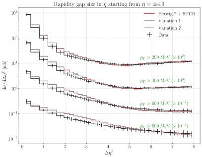
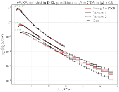
Figure 11: Predictions for the rapidity gap fraction and the pion, kaon, and proton yields as measured by Aad:2012pw and Adam:2015qaa . Variations in the spacetime components of the model show very little impact on the results.

Typical observables that are used to verify the description of MPI models in underlying event measurements are the angle of the particle production with respect to the leading track as well as the average sum of transverse momenta in the region towards, away, and transverse to the leading track. Comparing our model to data measured at the ATLAS collaboration Aad:2010fh , we find that the turn on behaviour, $p_{\perp}<2.5$ GeV for the leading track, is slightly too low. This has also been seen in the previous Herwig models. For leading tracks above $2.5$ GeV, the average transverse momentum sum is about 10% too large. This can also be seen in the radial dependence with respect to the leading track. In the Herwig MPI model, there is no azimuthal correlation between the additional scatters. Herwig’s only mechanism to correlate the additional scatters is the colour reconnection. Introducing methods to correlate these scatters, as well as correlate them angularly, is left to future work.

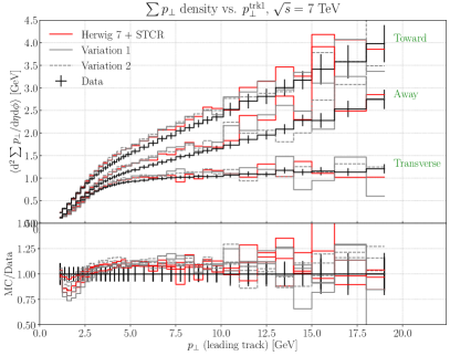
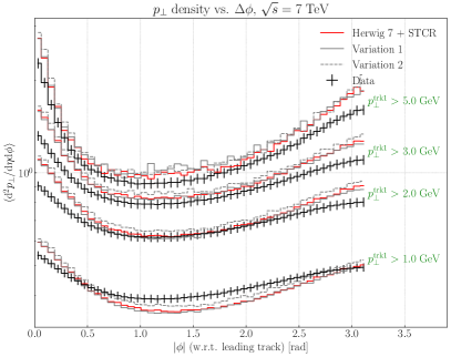
Figure 12: Predictions for the average sum of particle transverse momenta as a function of the leading track’s transverse momentum, and the average transverse momentum as a function of the azimuthal angle of the leading track Aad:2010fh .

8 Conclusion and Outlook

We have implemented spacetime coordinate generation for two stages of event simulation: the positions of MPI scattering centres, and the propagation distance in the transverse plane of partons at the end of the parton shower. We then used these transverse coordinates and the rapidity of the cluster constituents to define a measure that we minimize when performing baryonic colour reconnection, creating a model we call baryonic spacetime colour reconnection.

Overall we find that the proposed algorithm for baryonic spacetime colour reconnection gives meaningful results for many observables in Minimum Bias interactions at the LHC. This is an important step as with this prescription at hand we may explore larger systems, where spacetime structure will play an important role, as is the case in heavy ion collisions. However, we deliberately leave these new areas of study to future work after establishing the algorithm in $pp$ collisions in the first place.

There is plenty of room for future work based on the prescription we present here. One avenue might be to look at only allowing certain MPI subsystems to reconnect with each other based on closeness in spacetime Blok:2017pui . Alternatively, one may try to use the ideas of Gieseke:2018gff but limit the computation complexity of the problem by only performing the soft-gluon-evolution inspired colour reconnection in a small neighbourhood of spacetime.

One may also look to study the final state of the event in more detail using spacetime coordinates, an avenue started by Ferreres-Sole:2018vgo . One interesting idea is the interplay between Bose-Einstein correlations, and hadron position and extent Bialas:2013oza . Studying these effects could help one develop a more sophisticated and systematic model for generating spacetime coordinates.

As perturbative calculations become more precise, improving hadronization phenomenological models remains a key part of Monte Carlo event generator development. Overall, we have shown that it is possible to introduce spacetime coordinates and then use this information to help assist colour reconnection and potentially other soft physics phenomena.

Appendix A Formation time and mean lifetime

The discussion below is adapted from Dissertori:2003pj . For a branching of the kind $i\to jk$ where $j$ is the produced soft, collinear gluon, we start with the definition of $q_{i}$ and expand in terms of the products of the branching:

$$\begin{split}q_{i}^{2}&=\left(p_{j}+p_{k}\right)^{2}\\ &=2p_{j}\cdot p_{k}\\ &=2E_{j}E_{k}\left(1-\cos\theta\right)\\ &\sim E_{j}E_{k}\theta^{2}\\ &=\frac{E_{k}}{E_{j}}k_{\perp}^{2}\\ \mathrm{where}\;\;k_{\perp}&\coloneqq E_{j}\theta\end{split}$$ (18)

where in the second line we have assumed the products are massless, and the fourth line is the small angle approximation.

Using Eq. 8 for a virtual splitting parton, and ignoring the natural width term, one obtains:

$$\tau\sim\frac{1}{\sqrt{q_{i}^{2}}}.$$ (19)

Since Eq. 19 is defined in the rest frame of the decaying parton, the boost factor is:

$$\gamma=\frac{E_{i}}{\sqrt{q_{i}^{2}}}=\frac{E_{j}+E_{k}}{\sqrt{q_{i}^{2}}}$$ (20)

The lifetime in the lab frame is then:

$$\begin{split}\tau^{\prime}=\gamma\tau&\sim\frac{E_{j}+E_{k}}{\sqrt{q_{i}^{2}}}\frac{1}{\sqrt{q_{i}^{2}}}\\ &=(E_{j}+E_{k})\frac{E_{j}}{E_{k}}\frac{1}{k_{\perp}^{2}}\\ &=\frac{E_{j}}{k_{\perp}^{2}}\end{split}$$ (21)

where we have used the result of Eq. 18 in the second line, and in the last line we have used the soft approximation: $E_{j}\ll E_{k}$, i.e. a very soft gluon produced from a splitting where the quark takes most of the energy and momentum.

The final expression in Eq. 21 is the standard expression for the formation time of a massless soft, collinear gluon (see Baier:2000mf ; Casalderrey-Solana2016 ; Blaizot:2019muz ; Dominguez:2019ges for more details).

References

- (1) M. Bähr et al. Eur. Phys. J. C58 (2008) 639–707, [arXiv:0803.0883].
- (2) J. Bellm et al. arXiv:1705.06919.
- (3) J. Bellm et al. Eur. Phys. J. C76 (2016), no. 4 196, [arXiv:1512.01178].
- (4) T. Sjöstrand, S. Ask, J. R. Christiansen, R. Corke, N. Desai, P. Ilten, S. Mrenna, S. Prestel, C. O. Rasmussen, and P. Z. Skands Comput. Phys. Commun. 191 (2015) 159–177, [arXiv:1410.3012].
- (5) T. Gleisberg, S. Hoeche, F. Krauss, M. Schönherr, S. Schumann, F. Siegert, and J. Winter JHEP 02 (2009) 007, [arXiv:0811.4622].
- (6) T. Sjöstrand and M. van Zijl Phys. Rev. D36 (1987) 2019.
- (7) J. M. Butterworth, J. R. Forshaw, and M. H. Seymour Z. Phys. C72 (1996) 637–646, [hep-ph/9601371].
- (8) M. Bahr, S. Gieseke, and M. H. Seymour JHEP 07 (2008) 076, [arXiv:0803.3633].
- (9) M. Bähr, J. M. Butterworth, S. Gieseke, and M. H. Seymour in Proceedings, 1st International Workshop on Multiple Partonic Interactions at the LHC (MPI08): Perugia, Italy, October 27-31, 2008, pp. 239–248, 2009. arXiv:0905.4671.
- (10) S. Gieseke, F. Loshaj, and P. Kirchgaeßer Eur. Phys. J. C77 (2017), no. 3 156, [arXiv:1612.04701].
- (11) T. Sjöstrand and V. A. Khoze Z. Phys. C62 (1994) 281–310, [hep-ph/9310242].
- (12) S. Gieseke, C. Röhr, and A. Siodmok Eur. Phys. J. C72 (2012) 2225, [arXiv:1206.0041].
- (13) C. Bierlich and J. R. Christiansen Phys. Rev. D92 (2015), no. 9 094010, [arXiv:1507.02091].
- (14) S. Gieseke, P. Kirchgaeßer, and S. Plätzer Eur. Phys. J. C78 (2018), no. 2 99, [arXiv:1710.10906].
- (15) J. R. Christiansen and P. Z. Skands JHEP 08 (2015) 003, [arXiv:1505.01681].
- (16) T. Sjöstrand 2013. arXiv:1310.8073.
- (17) L. Lönnblad Z. Phys. C70 (1996) 107–114.
- (18) S. Gieseke, P. Kirchgaeßer, S. Plätzer, and A. Siodmok JHEP 11 (2018) 149, [arXiv:1808.06770].
- (19) J. Bellm Eur. Phys. J. C78 (2018), no. 7 601, [arXiv:1801.06113].
- (20) J. D. Bjorken FERMILAB-PUB-82-059-THY.
- (21) M. Gyulassy and M. Plumer Phys. Lett. B243 (1990) 432–438.
- (22) G.-Y. Qin and X.-N. Wang Int. J. Mod. Phys. E24 (2015), no. 11 1530014, [arXiv:1511.00790]. [,309(2016)].
- (23) C. Bierlich, G. Gustafson, L. Lönnblad, and A. Tarasov JHEP 03 (2015) 148, [arXiv:1412.6259].
- (24) C. Bierlich, G. Gustafson, and L. Lönnblad arXiv:1612.05132.
- (25) J. R. Ellis and K. Geiger Nucl. Phys. A590 (1995) 609C–612C, [hep-ph/9503212].
- (26) S. Ferreres-Solé and T. Sjöstrand Eur. Phys. J. C78 (2018), no. 11 983, [arXiv:1808.04619].
- (27) B. Andersson, G. Gustafson, G. Ingelman, and T. Sjöstrand Phys. Rept. 97 (1983) 31–145.
- (28) C. Bierlich and C. O. Rasmussen arXiv:1907.12871.
- (29) P. Aurenche, F. W. Bopp, A. Capella, J. Kwiecinski, M. Maire, J. Ranft, and J. Tran Thanh Van Phys. Rev. D45 (1992) 92–105.
- (30) B. Webber Nuclear Physics B 238 (1984), no. 3 492 – 528.
- (31) D. Amati and G. Veneziano Physics Letters B 83 (1979), no. 1 87 – 92.
- (32) S. Kirkpatrick, C. D. Gelatt, and M. P. Vecchi Science 220 (1983), no. 4598 671–680.
- (33) G. C. Fox and S. Wolfram Nucl. Phys. B168 (1980) 285–295.
- (34) J. R. Ellis and K. Geiger Phys. Rev. D54 (1996) 1967–1990, [hep-ph/9511321].
- (35) J. R. Ellis, K. Geiger, and H. Kowalski Phys. Rev. D54 (1996) 5443–5462, [hep-ph/9605425].
- (36) G. Corcella, I. G. Knowles, G. Marchesini, S. Moretti, K. Odagiri, P. Richardson, M. H. Seymour, and B. R. Webber JHEP 01 (2001) 010, [hep-ph/0011363].
- (37) S. Gieseke, P. Stephens, and B. Webber JHEP 12 (2003) 045, [hep-ph/0310083].
- (38) S. Platzer and S. Gieseke JHEP 01 (2011) 024, [arXiv:0909.5593].
- (39) R. Baier, D. Schiff, and B. G. Zakharov Ann. Rev. Nucl. Part. Sci. 50 (2000) 37–69, [hep-ph/0002198].
- (40) J. Casalderrey-Solana, D. Pablos, and K. Tywoniuk Journal of High Energy Physics 2016 (Nov, 2016) 174.
- (41) J.-P. Blaizot and F. Dominguez Phys. Rev. D99 (2019), no. 5 054005, [arXiv:1901.01448].
- (42) F. Domínguez, J. G. Milhano, C. A. Salgado, K. Tywoniuk, and V. Vila arXiv:1907.03653.
- (43) G. S. Bali Phys. Rev. D62 (2000) 114503, [hep-lat/0006022].
- (44) D. Reichelt, P. Richardson, and A. Siodmok Eur. Phys. J. C77 (2017), no. 12 876, [arXiv:1708.01491].
- (45) C. Röhr, Colour Charge Effects in Hadronization. Diplomarbeit, Karlsruhe Institute of Technology, 2010.
- (46) J. Bellm, S. Gieseke, and P. Kirchgaesser arXiv:1911.13149.
- (47) J. Bellm and L. Gellersen arXiv:1908.10811.
- (48) A. Buckley, J. Butterworth, L. Lönnblad, D. Grellscheid, H. Hoeth, J. Monk, H. Schulz, and F. Siegert Comput. Phys. Commun. 184 (2013) 2803–2819, [arXiv:1003.0694].
- (49) A. Buckley, H. Hoeth, H. Lacker, H. Schulz, and J. E. von Seggern Eur. Phys. J. C65 (2010) 331–357, [arXiv:0907.2973].
- (50) A. Donnachie and P. V. Landshoff Phys. Lett. B296 (1992) 227–232, [hep-ph/9209205].
- (51) CDF Collaboration, F. Abe et al. Phys. Rev. D50 (1994) 5550–5561.
- (52) A. Donnachie and P. V. Landshoff Phys. Lett. B595 (2004) 393–399, [hep-ph/0402081].
- (53) ALICE Collaboration, J. Adam et al. Eur. Phys. J. C75 (2015), no. 5 226, [arXiv:1504.00024].
- (54) ALICE Collaboration, B. Abelev et al. Eur. Phys. J. C73 (2013), no. 6 2456, [arXiv:1208.4968].
- (55) ATLAS Collaboration, G. Aad et al. New J. Phys. 13 (2011) 053033, [arXiv:1012.5104].
- (56) ATLAS Collaboration, G. Aad et al. Phys. Rev. D83 (2011) 112001, [arXiv:1012.0791].
- (57) CMS Collaboration, V. Khachatryan et al. Phys. Rev. D92 (2015), no. 1 012003, [arXiv:1503.08689].
- (58) C. B. Duncan and P. Kirchgaeßer Eur. Phys. J. C79 (2019), no. 1 61, [arXiv:1811.10336].
- (59) ATLAS Collaboration, G. Aad et al. Eur. Phys. J. C72 (2012) 1926, [arXiv:1201.2808].
- (60) B. Blok, C. D. Jäkel, M. Strikman, and U. A. Wiedemann JHEP 12 (2017) 074, [arXiv:1708.08241].
- (61) A. Bialas and K. Zalewski Phys. Lett. B727 (2013) 182–184, [arXiv:1309.6169].
- (62) G. Dissertori, I. G. Knowles, and M. Schmelling, High energy experiments and theory. 2003.