The mass-radius relation for neutron stars in gravity: a comparison between purely metric and torsion formulations
Abstract
Within the framework of gravity, we study realistic models of neutron stars, using equations of state compatible with the LIGO constraints. i.e. APR4, MPA1, SLy, and WW1. By numerically solving modified Tolman-Oppenheimer-Volkoff equations, we investigate the Mass–Radius relation in both metric and torsional gravity models. In particular, we observe that torsion effects decrease the compactness and total mass of neutron star with respect to the General Relativity predictions, therefore mimicking the effects of a repulsive massive field. The opposite occurs in the metric theory, where mass and compactness increase with , thus inducing an excess of mass that overtakes the standard General Relativity limit. We also find that the sign of must be reversed whether one considers the metric theory (positive) or torsion (negative) to avoid blowing up solutions. This could draw an easy test to either confirm or discard one or the other theory by determining the sign of parameter .
pacs:
11.30.-j; 04.50.Kd; 97.60.Jd.I Introduction
Compact objects, such as Neutron Stars (NS), are astrophysical objects that can be described by General Relativity (GR). These relativistic stars are natural laboratories for studying the behavior of high-density nuclear matter using an appropriate equation of state (EoS), which relates the pressure and density of degenerate matter. This allows one to obtain the Mass-Radius relation, , and other macroscopic properties such as the tidal deformability and the stellar momentum of inertia Steiner:2014pda .
Since the internal structure of a NS cannot be reproduced in the laboratory because of the extreme conditions in which it operates, only theoretical models can be formulated where there are a very large number of EoS candidates. The astrophysical measurements of the macroscopic properties of NS are very useful because they allow us to understand what can be realistic EoS . In fact, they can provide information on whether the EoS is soft or stiff and what is the pressure several times the density of nuclear saturation Lattimer:2015nhk ; Hebeler:2013nza ; Ozel:2016oaf ; Steiner:2017vmg . Therefore, measuring the mass value of a NS could help us to describe matter at extreme gravity regimes.
Einstein’s theory describe accurately the physical properties that govern the stability of NS where Chandrasekhar, considering degenerate matter, fixed a theoretical upper limit of so that the stability of a non-rotating degenerate star is conserved Chandrasekhar:1931ih . Instead, as confirmed by several astrophysical observations, there exist binary systems with NS having mass values that violates this limit allowing larger masses Barziv:2001ad ; Rawls:2011jw ; Mullally:2009rr ; Nice:2005fi ; 2010Natur.467.1081D ; Bao .
To study these observational evidences, as already done in some previous works, developed in metric formalism, capquark ; Astashenok:2013vza ; Astashenok:2014pua ; Astashenok:2014gda ; Astashenok:2014nua ; Capozziello:2015yza , Extended Theories of Gravity Capozziello:2011et ; dagostino can be used. In particular gravity, i.e. a class of Lagrangians considering a generic function of the Ricci curvature scalar. The primary objective is to obtain the relation for a NS that allows, given an EoS, to derive the maximum mass value.
From a cosmological point of view, theories, beside addressing in a straightforward way the inflationary paradigm Starobinsky:1980te , could be useful in view of problems like the accelerated expansion of the universe (the issue), confirmed by several observations Perlmutter:1998np ; Riess:1998cb ; Riess:2004nr ; Spergel:2006hy ; Schimd:2006pa ; McDonald:2004eu , and the problem of the formation of large-scale structures, called . Unlike the standard Concordance Lambda Cold Dark Matter (CDM) Model Bahcall:1999xn ; Bamba ; Joyce , similar results can be obtained without considering dark components but extending the gravitational sector at infrared scales Capozziello:2002rd ; Capozziello:2003tk ; Nojiri:2003ft ; Carroll:2003wy ; Olmo:2011uz ; Nojiri:2010wj ; Capozziello:2010zz ; Capozziello:2011et ; delaCruzDombriz:2012xy . Specifically, gravity is acquiring a growing interest because it allows a good description of gravitating structures without non-baryonic dark matter: extra degrees of freedom of gravitational field can be dealt as effective scalar fields contributing to the structure formation and stability Capozziello:2012ie ; Cembranos:2008gj . In this perspective, it is possible to unify the cosmic acceleration Capozziello:2002rd ; delaCruzDombriz:2006fj , the early-time inflation Starobinsky:1980te ; Planck:2013jfk , thus leading to a complete picture of the evolution of the Universe Nojiri:2003ft ; Ferrara ; Sebastiani ; Bamba2 ; Bamba3 ; Nojiri3 ; Elizalde and large-scale structures therein delaCruzDombriz:2008cp ; Abebe ; Abebe2 ; Oikonomou . However, the dark side and the descriptions are, in some sense, equivalent at large scale so one needs an experimentum crucis capable of discriminating among the two competing pictures. Discovering new particles out of the Standard Model or addressing gravitational phenomena that escape from the GR description could be an approach to fix this challenging issue. Observing exotic stars modeled by some alternative theory of gravity could be a goal in this perspective.
In this paper, we derive the diagram, using realistic EoS compatible with the LIGO constraints TheLIGOScientific:2017qsa for a Lagrangian, using two different approaches: the purely metric theory and a theory with torsion that allows one to introduce the spin degrees of freedom in GR Hehl:1976kj . In our specific model, the torsion field is due to the non-linearity of . Here the mass-energy is the source of curvature and the spin is the source of torsion. In this way, torsion contributions could provide additional information for compact stars in extreme gravity regimes.
The goal of this paper is to obtain realistic relation by solving numerically a modified system of equations, derived from Tolman-Oppenheimer-Volkoff (TOV) Oppenheimer:1939ne equations, and compare results with the LIGO constraints. Specifically, we shall consider quadratic corrections to the Ricci scalar and discuss models with and without torsion comparing them with GR.
The paper is organized as follows. In Section II we derive the TOV equations for gravity in the metric and torsion formalism. Section III is devoted to the problems related to the numerical aspects of TOV equations in gravity. In Section IV we derive the numerical solutions of stellar structure equations and compare the results of the relations. Discussion and conclusions are given in Sec. V.
II Tolman-Oppenheimer-Volkov equations in gravity
II.1 The metric theory
In the metric formulation, the action for gravity (in units for ) is given by
| (1) |
where is a function of the scalar curvature , is determinant of the metric tensor and is the matter Lagrangian. Varying the action (1) with respect to the metric tensor , one gets the field equations:
| (2) |
In eqs. (2), is the Ricci tensor, denotes the derivative of with respect to the scalar curvature, is the energy–momentum tensor of matter and indicates the covariant d’Alembert operator. Here we adopt the signature .
In order to describe stellar objects, we assume that the metric is static and spherically symmetric of the form:
| (3) |
where and are functions depending only on the radial coordinate . We assume that the interior of the star matter is described by a perfect fluid, with energy–momentum tensor , where and are the matter density and pressure respectively.
By a direct calculation, it is possible to show that field eqs. (2), evaluated in the metric (3), are equivalent to a set of equations consisting of the Tolmann-Oppenheimer-Volkov (TOV) equations for gravity and a continuity equation given by the contracted Bianchi identity . Specifically, the TOV equations for gravity are
| (4) |
| (5) |
while the continuity equation is
| (6) |
Here and denote respectively the first and second derivative of with respect to radial coordinate . In order to solve numerically the equations (4), (5) and (6), we can consider the scalar curvature as an independent dynamical field. In doing this, we need an additional equation which is directly obtained form the definition of scalar curvature:
| (7) |
Indeed, inserting the content of eqs. (4), (5) and (6) into (7), we get the dynamical equation for :
| (8) |
Finally, the numerical solution of the resulting dynamical equations relies on the assignment of a suitable EoS, , relating pressure and density inside the star, as well as of initial data (i.e. values of the fields at the center of the star).
II.2 The theory with torsion
In gravity with torsion, the gravitational and dynamical fields are pairs (, ) consisting of a pseudo-Riemannian metric and a metric compatible linear connection with non–vanishing torsion.
The corresponding field equations are obtained by varying the action functional (1) independently with respect to the metric and the connection. It is worth noticing that now refers to the scalar curvature associated with the dynamical connection .
Moreover, we recall that any metric compatible linear connection may be decomposed as the sum
| (9) |
where is the Levi–Civita connection associated with the given metric and denotes the contorsion tensor, related to the torsion tensor by the relation Hehl:1971qi :
| (10) |
The contorsion tensor (10) verifies the antisymmetry property and, together with the metric tensor , identifies the actual degrees of freedom of the theory.
Making use of eqs. (9) and (10), we can decompose the Ricci and the scalar curvature of the dynamical connection respectively as:
| (11) |
and
| (12) |
where and are the Ricci and the scalar curvature of the Levi–Civita connection induced by the metric .
In the absence of matter spin density, variations of (1) yield the field equations Capozziello:2007tj ; Capozziello:2008yx ; Capozziello:2008kb ; Capozziello:2010iy ; Capozziello:2010 :
| (13) |
and
| (14) |
where denotes again the energy-momentum tensor of matter, and the non–linearity of the gravitational Lagrangian function becomes a source of torsion.
Now, by inserting eqs. (11) and (14) into eqs. (13), it is possible to show that the whole set of field equations evaluated in the metric (3) is equivalent to the system formed by the following two TOV equations
| (15) |
Also in the torsional case, we consider the scalar curvature as an independent dynamical variable, introducing a consequent additional equation derived from the very definition of itself. In fact, inserting eqs. (10) and (14) into (12), evaluating all in the metric (3) and making use of eqs. (15) and (16), we obtain the evolution equation:
| (18) |
Again, in order to be solved, the set of dynamical equations (15), (16), (17) and (18) for the unknowns and must be completed by an EoS and initial data.
II.3 The model
We consider here the specific form of :
| (19) |
where is the coupling parameter of the quadratic curvature correction. This model is specially suitable to account for cosmological inflation, where higher-order curvature terms naturally lead to cosmic accelerated expansion. The quadratic term emerges in strong gravity regimes, while at Solar System scales and, more in general, in the weak field regime, the linear term predominates.
This statement can be easily demonstrated because any analytic model, in the weak field limit, presents a Yukawa-like correction in the gravitational potential except for where only the Newtonian potential is recovered. As shown in New1 ; New2 , such a correction is relevant at very large scales (e.g. at galactic scales and beyond Capozziello:2012ie ) with respect to Solar System and does not affect classical experimental constraints of GR. As a consequence, terms are relevant only in the strong field regime.
Since the interior of a NS could present energy conditions in some sense similar to those early universe Astashenok:2014pua , the model (19) is particularly suitable for our considerations. In this model, eqs. (4), (5) and (8) take the explicit form:
| (20) |
| (21) |
| (22) |
while eqs. (15), (16) and (18) become respectively:
| (23) |
| (24) |
| (25) |
Clearly the torsion contributions emerge in the second system. In the next Section, we shall discuss numerical solutions for the interior space–time of spherically symmetric NS in both metric and torsional gravity. Our aim is to compare the solutions of the above two systems of differential equations in order to point out the torsion contribution with respect to the purely metric one.
In view of this, it is worth noticing that, in vacuo, gravity with torsion amounts to GR Capozziello:2007tj ; Capozziello:2010 . Therefore, under the assumption of spherical symmetry, in the case with torsion, the space–time outside the star has to coincide with the Schwarzschild one. In order to compare the two models, it is then reasonable and consistent assuming the external Schwarzschild solution as the space–time outside the star also in the case of purely metric theory. It is worth noticing that the Schwarzschild external solution is actually a vacuum solution for purely metric gravity as demonstrated in Whitt ; Mignemi .
Therefore, viable interior solutions, at the boundary, have to match the external Schwarzschild solution. In this regard, we recall that junction conditions for gravity have been studied in Deruelle for the purely metric formulation, and in VCC ; CV1 ; CV2 for the theory with torsion. Referring the reader to Deruelle ; VCC for more details, we assume the following junction conditions at the stellar radius
| (26) |
| (27) |
Outside the star , and refer to the corresponding Schwarzschild quantities. Eqs. (26) and (27) are the conditions at the stellar radius to be satisfied by the numerical solutions we shall investigate in the next Sections.
III Numerical aspects of the TOV equations in gravity
The TOV equations presented in Sec. II, together with an EoS, form a closed system of equations that can be solved numerically once a suitable set of initial conditions are provided. The EoS accounts for the behavior of the matter fields in the NS at nuclear level. However, it also dominates the NS macroscopic properties as the total mass , radius and compactness . The total mass and the radius may vary significantly depending on the state of matter in the NS interior where , being the black hole solution. On the other hand, the knowledge of the macroscopic properties provides a direct insight to understand the particle interactions, energy transport and state of the matter in the NS core. Until recently, there were placed only vague constraints on the EoS of NSs from electromagnetic observations Radice:2017lry . The recent LIGO-Virgo binary neutron star (BNS) observation has significantly clarified the state of art concerning the EoS physics. The largest accuracy of the gravitational wave (GW) channel in relation to the electromagnetic (EM) observations allowed to rule out stiffer solutions (less compact) thus reducing significantly the number of astrophysically relevant EoS. In this section, we discuss some aspects of the numerical solution of TOV equations in the metric and torsional , formulations described above, for four EoS compatible with the recent LIGO constraints: APR4, MPA1, SLy, WFF1 Alford:2004pf ; Mueller:1996pm ; Douchin:2001sv ; Wiringa:1988tp , accurately described the piecewise polytropic fits provided in Read:2009yp .
Then, to solve numerically the TOV equations, we use a dimensionless version of the them by re-scaling our physical variables as
| (28) |
where
| (29) |
and is the mass of the sun, is the gravitational radius (), Newton’s Gravitational constant and the speed of light. The two systems of differential equations shown in Subsection II.3 take the following form,
| (30) |
where the primed variables denote radial derivatives. Therefore, we are left to setup five initial conditions (ICs) for the variables to complete the numerical scheme. ICs are chosen at the center of the star in order to preserve regularity, thus preventing the generation of large gradients that may lead to numerical instabilities. Mathematically, this involves that any expansion around the NS center must have a zero first derivative. In particular, the scalar curvature at the NS center may be expanded as,
| (31) |
where regularity involves . Pressure and density at the center and are given by the EoS so they only depend on the type of fluid under consideration. For the metric potential , it is natural to fix , analogously to what happens in Newtonian gravity, where the and variables are matched to the mass of the system by,
| (32) |
Notice that the variable does not enter directly in our system of differential equations which implies that can be defined up to any arbitrary constant. Therefore we adjust conveniently to match (i) the internal solutions with the external Schwarzschild solution at the stellar radius and (ii) to obtain asymptotically the profile as,
| (33) |
The star radius is ideally defined where the pressure though, in practice, and for numerical reasons, it is sufficient to set a ground value as .
The fulfillment of eqs. (33) requires to find an optimal choice for the Ricci scalar . In general, this is achieved by shooting the central value within some sufficiently large range , containing the true value . Then is found by applying bijection root-finding methods until eqs. (33) are satisfied up to numerical tolerance. Unfortunately, the existence of such strongly depends on the particular form of the model, giving rise to ghosts in case of ill-defined configuration of the model parameters. This is true for both metric and torsional theories discussed in this work. Then we choose the sign of to be the one that better matches the junction conditions at the surface of the star (26), (27) for the metric and torsional theory respectively. As we evince in the following sections, the only choices that reproduce not blowing up solutions are for the metric case and for the torsion one. Unfortunately, these choices generate some typical tachyonic oscillations due to a bad behaved and that we could not remove numerically. This effect was also reported in Resco:2016upv and it shows an oscillatory behavior, in the form of a damped-sinusoid outside the star, even in the minimally perturbed scenario with . These oscillations grow as the value of increases and they are as well propagated to our metric potentials and . This inserts some ambiguity in defining the asymptotic conditions (33) for large since the oscillations are not totally vanished when the numerical noise begins to dominate the solution (for ). To overcome this issue and to reduce the amplitude of the oscillations, we restrict our analysis to small values of . As this is anyway consistent with current observational tests, in doing so, we are not discarding any relevant astrophysical scenario and this fact allows us to set . This hypothesis is shown to have a minimal impact in the diagrams as we will discuss throughout next sections. Moreover, the assumption of a Schwarzschild-type solution outside the star allows us to smooth out these oscillations and to recover a good fulfillment of the junction conditions. According to the above positions, we justify the choice of for the metric theory and for the torsional one.
Finally, the two systems of ordinary differential equations (ODE) are solved by using a -order Runge-Kutta with adaptive step-size and high-stiffness control methods implemented in the Wolfram Mathematica package Mathematica . These methods regulate the discretization step-size by estimating the error of the Runge-Kutta method point by point ensuring the numerical convergence of the solution step by step. The stiffness control methods use polynomial extrapolation on the short regimes where the gradients become too large. We have found these methods essential to ensure the accuracy of the solutions in the torsional formulation.
IV Numerical solutions
We compute the diagrams for metric and torsional formulations of gravity. Due to the numerical limitations found throghout our analysis, we restrict where is required to be positive for the purely metric theory and negative in the theory with torsion to avoid blowing up solutions Resco:2016upv . These values are anyway consistent with solar system tests of GR Resco:2016upv ; Lombriser:2011zw . Such tests fix light constraints on the form rather than on the parameter , thus being translated as . Bearing in mind that curvatures themselves are expected to be small, this leaves the parameter rather unconstrained. Other tests as Eöt-Wash laboratory experiment set . On the contrary, there exist alternative observational space-based constraints coming from the Gravity Probe B experiment Everitt:2011hp or the observation of the binary pulsar PSR J0737-3039 Breton:2008xy ; Naf:2010zy that set . Therefore, the discrepancies among the several experiments do not set tight bounds on the value of , and our choice seems to be compatible with existing data.

IV.1 Purely metric theory
The solutions of the TOV equations for the purely metric model are illustrated in Figure 1. The pressure at the center of the star drops quickly until it eventually gets equal to zero, thus defining the radius of the star . This radius is used as our reference point to compute the total mass by means of eq. (32).
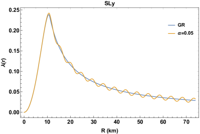
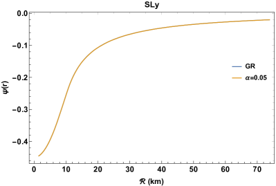
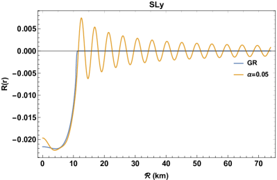
The numerical system exhibits some dissipative oscillations about the Ricci scalar and the metric potential . These oscillations naturally arise from the harmonic-form of the Ricci scalar equation in vacuum Resco:2016upv , for a non optimal choice of the Ricci scalar at the center of the star, and where optimal choice is here defined as that matching the Schwarzschild junction conditions at the stellar radius. Unfortunately, such a choice becomes increasingly difficult as tends to zero since the system of equations become also stiffer Doneva:2013rha . Generally speaking, this may appear to be counterintuitive, since should exactly recover the GR space-time. However the asymptotic approach to of the Ricci scalar equations (22)(25) are ill-defined. This is clear if, for instance, one re-expresses (22) as,
| (34) |
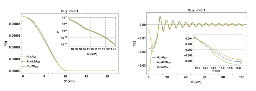
Notice that the numerator of the first term is exactly zero in GR and that ideally approaches to zero faster than linear order in . However, this is not so exact when dealing with numerical uncertainties, where the same factor may behave as a solution for thus requiring much more precision on the estimation of central value . To overcome this issue, we have set to the GR value. Though this seems apparently an arbitrary choice, we notice that, for , the solution must be close to GR so the value cannot be further to that of GR. This is self-evident from Fig. 2, where, in the right plot, we illustrate the variations on the pressure and the Ricci scalar for different choices of the central value . Then, notice than the effect of varying on the radius for such small values of is about considering the maximum and minimum choices of . This variation is then compared with the uncertainty arising from the definition of the star radius to be the place where the pressure drops by a factor . Then, in the left plot, we show that the impact of relaxing this value to would generate an uncertainty of about , thus larger than the one from varying .
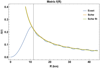


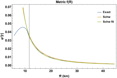
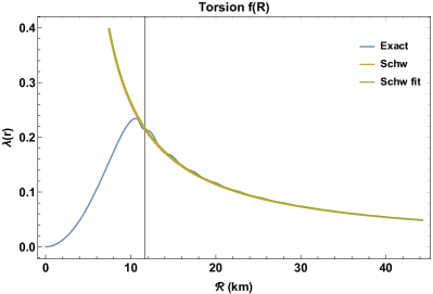
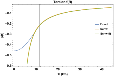
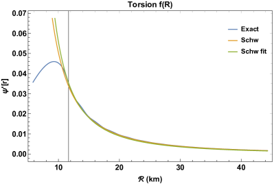
In Fig. (3), we show the behavior of the metric potentials and and the derivatives and paying special attention to: (i) the junction conditions at the NS boundary and (ii) their profiles as . We show the full numerical solution (blue line), its corresponding Schwarzschild solution (orange line) given by eqs. (32) with and the result of fitting the exterior data to the same Schwarzschild-like ansatz in order to quantify the agreement with the Schwarzschild solution outside the star and which results in a NS with total mass . The good agreement between the three lines confirms that the solution is well approximated by the Schwarzschild solution right outside the star radius better than . This good match is also extended to their derivatives thus globally satisfying the necessary junction conditions of eqs. (26) once the oscillations are averaged out. On the other hand, since the oscillations do not appear on , we choose this quantity more appropriated to define the NS mass .

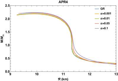
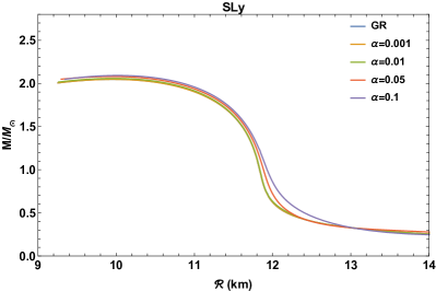
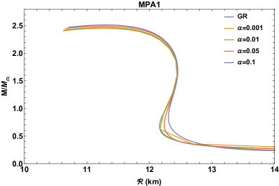
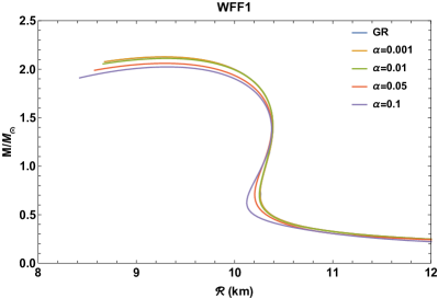
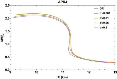
Finally, in Fig. 4, we show the diagrams for the four EoS considered in this work. For each choice of the central density , we get a different estimate of the radius and the total mass . We loop over until which defines the unstable branch, i.e. the point at which the NS is expected to collapse to a black hole and that provides the maximum allowed mass for the given EoS. Note that for all the EoS considered, the total mass tends to increase with respect to GR as in Doneva:2013rha ; Capozziello:2015yza ; sbisa . This is because gravity becomes stronger, thus allowing more massive systems. Indeed, in the scenario, Newton’s gravitational constant is replaced by
| (35) |
The combined conditions of and imply then , thus generating a more attractive gravity.
IV.2 Theory with torsion
We repeat the analysis for the torsional theory. Although further models have been also considered in the literature, the numerical complexity of torsional equations makes difficult a full exploration of other kinds of functions. This issue becomes more relevant when considering the torsional theory with spin Capozziello:2008yx , where spin gradients add higher order derivatives to our system of equations that increase the stiffness of the numerical system. We plan to extend our study in the presence of spin matter in a forthcoming paper.

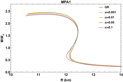
Then, in Figure 5, we show the results we obtained for the theory with torsion, using the same range for as in the metric case but choosing . In this scenario, we see that the general trend predicts a decreasing of the total mass of NS, independently of the EoS considered. This could be related with the fact that the stable branch of the solutions, given by the sign of , is reversed with respect to the purely metric case to avoid for ghosts. However, estimates for the total mass and radius are still compatible with the astrophysical observations Ozel:2016oaf , thus not allowing us to rule out any of the models studied here. On the other hand, if we further increase the errors generated by eq. (25) and propagated to the total mass and the total radius become too large. Therefore, we restrict our analysis to . In Fig. 6 we repeat the same Schwarzschild-based tests adopted for the metric formalism for . In this case, the total mass is slightly diminished with respect to the metric case. Notice that the Schwarzschild solution is as well verified at the star radius , where the metric is clearly and still preserves the condition. Outside the star, and once the oscillations are vanished, the metric functions and still preserve the decay.

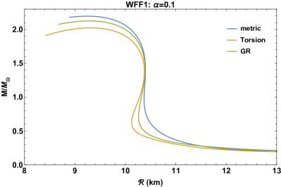
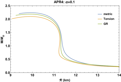


Finally, in Fig 7 we compare the different predictions obtained in the purely metric and the torsional formulation respectively, for . Note that, in the theory with torsion, though the total mass of the NS decreases, while increases with respect to the metric case, the relative deviations, in absolute value, with respect to GR seem to be larger than in the metric case. This is caused by the effective repulsion generated by the extra torsional terms (see eq. (25)) which induce a partial screening of the gravitational field that prevents to reach NS masses as large as in standard GR. This is explicitly shown in Table 1, where we show the variation of the maximum mass , radius and compactness for the purely metric and torsional theories respectively, corresponding to the points in the diagrams where . Note that whereas the purely metric formulation tends to more massive and compact NSs, the opposite occurs when considering torsion. Specifically, as the quadratic term in the curvature increases, the effects of torsion counterbalance the increase of total mass. This can be intuitively derived by using the same reasoning as in (35) with and , implying and thus generating a less attractive gravity.
The stability of the solutions can be checked adopting the so-called Regge-Wheeler-Zerilli formalism Regge ; Zerilli . As discussed in Nashed , perturbations in gravity models can be dealt by taking into account odd-type metric perturbations and stability of geodesic motion around the solution. In that case, a charged spherically symmetric black hole was considered and stability was strictly dependent on the value of parameters as the black hole mass, the cosmological constant and the electric charge. In the present case, the leading parameter is which determines the stability of solution . According to the values reported in Figs 4, 5, and 7, both for metric and torsional case, our numerical solutions result stable against perturbations. Specifically, the stability region is given by which determines the maximal stable configuration as discussed above.
An important remark is in order at this point to justify the result. According to the Regge, Wheeler Regge , and Zerilli Zerilli formalism, metric perturbations can be decomposed according to their transformation properties under two-dimensional rotations. These authors, originally, took into account perturbations of the Schwarzschild metric in GR, however, as shown in Nashed , the formalism depends on the properties of spherical symmetry and then can be easily applied to gravity.
If we consider the perturbed metric for a static spherically symmetric spacetime as , the tensor represents small perturbations with respect to the background. Under two-dimensional rotations, and transform as scalars, and transform as vectors and transforms as tensors ( are either or ). A scalar quantity is expressed in spherical harmonics as
| (36) |
Adopting the spherical symmetry, the solution is independent of , and then this subscript can be omitted and one can take into account only the index representing the multipole number arising from the separation of angular variables by the expansion into spherical harmonics, that is
| (37) |
A vector can be decomposed into a divergence part and a divergence-free part:
| (38) |
where and are two scalars and . Here is the two-dimensional metric on the sphere and is the totally anti-symmetric tensor with ; is the covariant derivative with respect to . Being a two-component vector, it is assigned by and . We can take into account the decomposition (36) for and to decompose the vector quantity into spherical harmonics. The variables related to are (axial) odd-type modes and the others are (polar) even-type modes. This decomposition is useful because, in the linearized equations of motion (or equivalently, in the second order action) for , odd-type and even-type perturbations are completely decoupled. This fact is due to the invariance of the background metric under parity transformations. Therefore, one can study odd-type and even-type perturbations separately. The difference between the two families is their parity. Under the parity operator a spherical harmonic with index transforms as . The polar perturbations transform, under parity, in the same way. On the other hand, the axial perturbations transform as . Adopting the Regge-Wheeler formalism, metric perturbations are
| (39) | |||
| (40) | |||
| (41) | |||
| (42) |
From the gauge transformation , where are infinitesimal quantities, one can show that some metric perturbations are not physical and then some of them can vanish. Specifically, we can consider the transformation:
| (43) |
where can always set to vanish. This is called the Regge-Wheeler gauge. According to this procedure, is fixed and there is no remaining gauge degrees of freedom. From this result, the only relevant perturbations are the odd-ones. See also Ganguly for details.
V Discussion and conclusions
In this paper, we have studied the existence of realistic NSs in the context of the theory both in purely metric and torsional formulations. The main results concern the computation of the diagrams resulting from the two different theoretical frameworks considered. Matter fields have been represented by static and spherically symmetric perfect fluids where the EoS have been chosen to agree with the recent LIGO-Virgo constraints TheLIGOScientific:2017qsa . The parameter has been restricted to be smaller than to avoid unrealistically large oscillations (see e.g. Resco:2016upv ) on our metric potentials and therefore ensuring the(i) fullfillment of junction conditions and (ii) the accurate recovery of the Schwarzschild solution far from the source. These two requirements single out four of the five initial conditions: , , and , while remains free. is ideally defined by choosing this parameter in such a way to match the junction conditions (26),(27). However, the oscillatory behavior of some solutions for prevents from finding a unique value for . To overcome this issue, we have set identical to the GR value. This assumption have been shown to be valid for small , being the estimates of the NS radius only mildly dependent on the choice, but this is no longer true for .
However, a general consideration is in order at this point to justify the assumption . Let us consider the trace of field equations in metric
| (44) |
and in torsion case
| (45) |
Substituting , we have, in the metric case,
| (46) |
and, in the torsion case,
| (47) |
For the metric picture, it is reasonable to suppose that, at the center of the star, because one can assume a constant central density without remarkable variations and gradients kippen . For the torsion picture, we recover exactly the trace of GR. According to these results, the assumption , besides the above numerical considerations, is fully justified.
In the purely metric theory, the obtained results show a progressive increasing of the total mass as increases, for all the four EoS considered. This allows for higher masses and more compact NSs than in GR. This absloute increasing of the mass and compactness could be also reproduced by assuming softer EoS in GR, consistent with the recent observations TheLIGOScientific:2017qsa . In the case with torsion, the NS mass tends to decrease for all the EoS considered. This could be related with the fact that the stable branch of the solutions is flipped with respect to the purely metric case to ensure the stability of the numerical system. The physical existence of such solutions could help us to describe NS compact or not, based on astrophysical observations, choosing the appropriate theory by simply constraining whether is positive or negative. In the torsional framework, the differences in the predictions with respect to GR are larger than those obtained in the purely metric case. As a consequence, the allowed intervals on are poles apart from the two theories. Moreover, the theory with torsion would seem to describe less compact NS. This would allow one to obtain solutions that could be reproduced using EoS with stiff matter in the limit of GR. Unfortunately, this is in disagreement with the recent LIGO-Virgo discoveries TheLIGOScientific:2017qsa . What comes to the rescue is that given the current accuracy of electromagnetic observations, we cannot deny the NS observations yet because the differences with the GR are still too small. However, this issues could be addressed by next generation gravitational wave detectors (3G) Sathyaprakash:2012jk ; Essick:2017wyl ; 2017arXiv170200786A , where the opportunity to test results presented in this work could be realistic.
| 0 | 2.13 | 9.29 | 0.23 | 2.13 | 9.29 | 0.23 | |
| 0.001 | 2.13 | 9.29 | 0.23 | 2.13 | 9.29 | 0.23 | |
| WWF1 | 0.01 | 2.14 | 9.28 | 0.23 | 2.11 | 9.30 | 0.23 |
| 0.05 | 2.19 | 9.21 | 0.24 | 2.06 | 9.28 | 0.22 | |
| 0.1 | 2.20 | 9.24 | 0.24 | 2.02 | 9.31 | 0.21 | |
| 0 | 2.19 | 9.88 | 0.22 | 2.19 | 9.88 | 0.22 | |
| 0.001 | 2.19 | 9.91 | 0.22 | 2.19 | 9.88 | 0.22 | |
| APR4 | 0.01 | 2.20 | 9.88 | 0.22 | 2.18 | 9.91 | 0.22 |
| 0.05 | 2.23 | 9.85 | 0.23 | 2.13 | 9.91 | 0.21 | |
| 0.1 | 2.24 | 9.92 | 0.23 | 2.10 | 9.91 | 0.21 | |
| 0 | 2.05 | 9.97 | 0.20 | 2.05 | 9.97 | 0.20 | |
| 0.001 | 2.05 | 9.94 | 0.20 | 2.05 | 9.94 | 0.20 | |
| SLy | 0.01 | 2.06 | 9.97 | 0.21 | 2.04 | 9.98 | 0.20 |
| 0.05 | 2.08 | 9.94 | 0.21 | 2.00 | 9.96 | 0.20 | |
| 0.1 | 2.10 | 10.02 | 0.21 | 1.98 | 9.98 | 0.20 | |
| 0 | 2.45 | 11.28 | 0.22 | 2.45 | 11.28 | 0.22 | |
| 0.001 | 2.45 | 11.30 | 0.22 | 2.45 | 11.26 | 0.22 | |
| MPA1 | 0.01 | 2.47 | 11.26 | 0.22 | 2.44 | 11.30 | 0.22 |
| 0.05 | 2.50 | 11.28 | 0.22 | 2.40 | 11.26 | 0.21 | |
| 0.1 | 2.51 | 11.30 | 0.22 | 2.37 | 11.26 | 0.21 |
Acknowledgements
We want to thanks Alvaro de la Cruz-Dombriz, Miguel Bezares Figueroa and Carlos Palenzuela for providing useful discussions on the numerical methods used in this work. SC acknowledges INFN Sez. di Napoli (Iniziative Specifiche QGSKY and MOONLIGHT2) for support. This article is also based upon work from COST action CA15117 (CANTATA), supported by COST (European Cooperation in Science and Technology).
References
- (1) A. W. Steiner, S. Gandolfi, F. J. Fattoyev, and W. G. Newton, Phys. Rev. C 91, 015804 (2015).
- (2) J. M. Lattimer and M. Prakash, Phys. Rept. 621, 127 (2016).
- (3) K. Hebeler, J. M. Lattimer, C. J. Pethick, and A. Schwenk, Astrophys. J. 773, 11 (2013).
- (4) F. Ozel and P. Freire, Ann. Rev. A&A 54, 401 (2016).
- (5) A. W. Steiner, C. O. Heinke, S. Bogdanov, C. Li, W. C. G. Ho, A. Bahramian, and S. Han, Mon. Not. Roy. Astron. Soc. 476, 421 (2018).
- (6) S. Chandrasekhar, Astrophys. J. 74, 81 (1931).
- (7) O. Barziv et al., A&A 377, 925 (2001).
- (8) M.L. Rawls et al., Astrophys. J. 730, 25 (2011).
- (9) F. Mullally, C. Badenes, S.E. Thompson and R. Lupton, Astrophys. J. 707, L51 (2009).
- (10) D. Nice et al., Astrophys. J. 634, 1242 (2005).
- (11) P.B. Demorest, T. Pennucci, S.M. Ransom, M.S.E. Roberts, J.W.T. Hessels, Nature 467, 1081 (2010).
- (12) Nai-Bo Zhang, Bao-An Li, Astrophys. J. 879, 99 (2019).
- (13) A. V. Astashenok, S. Capozziello, S. D. Odintsov, Physics Letters B 742, 160 (2015).
- (14) A. V. Astashenok, S. Capozziello and S. D. Odintsov, JCAP 1312, 040 (2013).
- (15) A. V. Astashenok, S. Capozziello and S. D. Odintsov, Phys. Rev. D 89, 103509 (2014).
- (16) A. V. Astashenok, S. Capozziello and S. D. Odintsov, Astrophys. Space Sci. 355, 333 (2015).
- (17) A. V. Astashenok, S. Capozziello and S. D. Odintsov, JCAP 1501, 001 (2015).
- (18) S. Capozziello, M. De Laurentis, R. Farinelli and S. D. Odintsov, Phys. Rev. D 93, 023501 (2016).
- (19) S. Capozziello and M. De Laurentis, Phys. Rept. 509, 167 (2011).
- (20) S. Capozziello, R. D’Agostino, O. Luongo, Int. J. Mod. Phys. D 28 1930016 (2019).
- (21) A. A. Starobinsky, Phys. Lett. B 91, 99 (1980).
- (22) S. Perlmutter et al. [Supernova Cosmology Project], Astrophys. J. 517, 565 (1999).
- (23) A. G. Riess et al. [Supernova Search Team], Astron. J. 116, 1009 (1998).
- (24) A. G. Riess et al. [Supernova Search Team], Astrophys. J. 607, 665 (2004).
- (25) D. N. Spergel et al. [WMAP Collaboration], Astrophys. J. Suppl. 148, 175 (2003).
- (26) C. Schimdt et al., Astron. Astrophys. 463, 405 (2007).
- (27) P. McDonald et al., (SDSS) Astrophys. J. Suppl. 163, 80 (2006).
- (28) N.A. Bahcall et al., Science 284, 1481 (1999).
- (29) K. Bamba, S. Capozziello, S. Nojiri, S.D. Odintsov, Astrophys.Space Sci. 342, 155 (2012).
- (30) A. Joyce, B. Jain, J. Khoury, M. Trodden, Phys.Rept. 568, 98 (2015).
- (31) S. Capozziello, Int. J. Mod. Phys. D 11, 483 (2002).
- (32) S. Capozziello, S. Carloni, A. Troisi, Recent Res. Dev. Astron. Astrophys. 1, 625 (2003).
- (33) S. Nojiri, S.D. Odintsov, Phys. Rev. D 68, 123512 (2003).
- (34) S. M. Carroll, V. Duvvuri, M. Trodden and M. S. Turner, Phys. Rev. D 70, 043528 (2004).
- (35) G. J. Olmo, Int.J.Mod.Phys. D 20, 413 (2011).
- (36) S. Nojiri and S. D. Odintsov, Phys. Rept. 505, 59 (2011).
- (37) S. Capozziello and V. Faraoni, Beyond Einstein gravity: A Survey of gravitational theories for cosmology and astrophysics. Fundamental Theories of Physics. 170, Springer (2010), ISBN 978-94-007-0164-9.
- (38) A. de la Cruz-Dombriz and D. Saez-Gomez, Entropy 14, 1717 (2012).
- (39) S. Capozziello and M. De Laurentis, Annalen Phys. 524, 545 (2012).
- (40) J. A. R. Cembranos, Phys. Rev. Lett. 102, 141301 (2009).
- (41) A. de la Cruz-Dombriz and A. Dobado, Phys. Rev. D 74, 087501 (2006).
- (42) P. A. R. Ade et al. [Planck Collaboration], Astron. Astrophys. 571, A22 (2014).
- (43) S. Ferrara, A. Kehagias and A. Riotto, Fortsch. Phys. 62, 573 (2014).
- (44) L. Sebastiani, G. Cognola, R. Myrzakulov, S. D. Odintsov and S. Zerbini, Phys. Rev. D 89, 023518 (2014).
- (45) K. Bamba, R. Myrzakulov, S. D. Odintsov and L. Sebastiani, Phys. Rev. D 90, 043505 (2014).
- (46) K. Bamba, S. Nojiri, S. D. Odintsov and D. Saez-Gomez, Phys. Rev. D 90, 124061 (2014).
- (47) S. Nojiri, S. D. Odintsov and D. Saez-Gomez, Phys. Lett. B 681, 74 (2009).
- (48) E. Elizalde and D. Saez-Gomez, Phys. Rev. D 80, 044030 (2009).
- (49) A. de la Cruz-Dombriz, A. Dobado and A. L. Maroto, Phys. Rev. D 77, 123515 (2008).
- (50) A. Abebe, A. de la Cruz-Dombriz and P. K. S. Dunsby, Phys. Rev. D 88, 044050 (2013).
- (51) A. Abebe, M. Abdelwahab, A. de la Cruz-Dombriz and P. K. S. Dunsby, Class. Quant. Grav. 29, 135011 (2012).
- (52) S. Nojiri, S. D. Odintsov, V. K. Oikonomou, Phys. Rept. 692, 1 (2017).
- (53) B. Abbott et al. (Virgo, LIGO Scientific), Phys. Rev. Lett. 119, 161101 (2017).
- (54) F. W. Hehl, P. Von Der Heyde, G. D. Kerlick and J. M. Nester, Rev. Mod. Phys. 48, 393 (1976).
- (55) J.R. Oppenheimer & G.M. Volkoff Phys. Rev. 55, 374 (1939).
- (56) F. W. Hehl and B. K. Datta, J. Math. Phys. 12, 1334 (1971).
- (57) S. Capozziello, R. Cianci, C. Stornaiolo and S. Vignolo, Class. Quantum Grav. 24, 6417 (2007).
- (58) S. Capozziello, R. Cianci, C. Stornaiolo and S. Vignolo, Int. J. Geom. Meth. Mod. Phys. 5, 765 (2008).
- (59) S. Capozziello, R. Cianci, C. Stornaiolo and S. Vignolo, Phys. Scripta 78, 065010 (2008).
- (60) S. Capozziello, R. Cianci, M. De Laurentis and S. Vignolo, Eur. Phys. J. C 70, 341 (2010).
- (61) S. Capozziello and S. Vignolo, Ann. Phys. (Berlin) 19, 238 (2010).
- (62) S. Capozziello and S. Vignolo, Class. Quantum Grav. 26, 175013 (2009).
- (63) S. Capozziello and S. Vignolo, Int. J. Geom. Meth. Mod. Phys. 9, 1250006 (2012).
- (64) S. Capozziello, A. Stabile and A. Troisi, Phys. Rev. D 76, 104019 (2007).
- (65) S. Capozziello, A. Stabile and A. Troisi, Mod. Phys. Lett. A 24, 659 (2009).
- (66) B. Whitt, Phys. Lett. B 145, 176 (1984).
- (67) S. Mignemi and D. L. Wiltshire, Phys. Rev. D 46, 1475 (1992).
- (68) N. Deruelle, M. Sasaki and Y. Sendouda, Progress of Theoretical Physics 119, 237 (2008).
- (69) S. Vignolo, R. Cianci and S. Carloni, Class. Quantum Grav. 35, 095014 (2018).
- (70) D. Radice, A. Perego, F. Zappa, and S. Bernuzzi, Astrophys. J. 852, L29 (2018).
- (71) M. Alford, M. Braby, M. W. Paris, and S. Reddy, Astrophys. J. 629, 969 (2005).
- (72) H. Mueller and B. D. Serot, Nucl. Phys. A606, 508 (1996).
- (73) F. Douchin and P. Haensel, Astron. Astrophys. 380, 151 (2001).
- (74) R. B. Wiringa, V. Fiks, and A. Fabrocini, Phys. Rev. C 38, 1010 (1988).
- (75) J. S. Read, C. Markakis, M. Shibata, K. Uryu, J. D. E. Creighton, and J. L. Friedman, Phys. Rev.D 79, 124033 (2009).
- (76) M. Aparicio Resco, A. de la Cruz Dombriz, F. J. Llanes Estrada, and V. Zapatero Castrillo, Phys. Dark Univ. 13, 147 (2016).
- (77) T. Regge and J. A. Wheeler, Phys. Rev. 108, 1063 (1957).
- (78) F. J. Zerilli, Phys. Rev. Lett. 24, 737 (1970).
- (79) G. G. L. Nashed and S. Capozziello, Phys. Rev. D 99, 104018 (2019).
- (80) A. Ganguly, R. Gannouji, M. Gonzalez-Espinoza, C. Pizarro-Moya, Class. Quant. Grav. 35, 145008 (2018)
- (81) W. R. Inc., Mathematica, Version 11.3, champaign, IL, 2018.
- (82) L. Lombriser, et al., Phys. Rev. D 85, 102001 (2012).
- (83) C. W. F. Everitt et al., Phys. Rev. Lett. 106, 221101 (2011).
- (84) R. P. Breton, V. M. Kaspi, M. Kramer, M. A. McLaughlin, M. Lyutikov, S. M. Ransom, I. H. Stairs, R. D. Ferdman, F. Camilo, and A. Possenti, Science 321, 104 (2008).
- (85) J. Näf and P. Jetzer, Phys. Rev. D 81, 104003 (2010).
- (86) D.D. Doneva, et al., Astrophys. J. 781, L6 (2013).
- (87) F. Sbisà, et al., Physics of the Dark Universe 27 C, 100411 (2020).
- (88) B. Sathyaprakash et al., Class. Quant. Grav. 29, 124013 (2012).
- (89) R. Essick, S. Vitale, and M. Evans, Phys. Rev. D 96, 084004 (2017).
- (90) P. Amaro-Seoane, et al., ArXiv 1702.00786 (2017).
- (91) R. Kippenhahn, A. Weigert, A. Weiss, Stellar Structure and Evolution, Springer, Dordrecht (2012).