1 Introduction

A variety of applications spanning science and engineering use Markov reward processes as models for real-world phenomena, including queuing systems, transportation networks, robotic exploration, game playing, and epidemiology. In some of these settings, the underlying parameters that govern the process are known to the modeler, but in others, these must be estimated from observed data. A salient example of the latter setting, which forms the main motivation for this paper, is the policy evaluation problem encountered in Markov decision processes (MDPs) and reinforcement learning [Ber95a, Ber95b, SB18]. Here an agent operates in an environment whose dynamics are unknown: at each step, it observes the current state of the environment, and takes an action that changes its state according to some stochastic transition function determined by the environment. The goal is to evaluate the utility of some policy—that is, a mapping from states to actions, where utility is measured using rewards that the agent receives from the environment. These rewards are usually assumed to be additive over time, and since the policy determines the action to be taken at each state, the reward obtained at any time is simply a function of the current state of the agent. Thus, this setting induces a Markov reward process (MRP) on the state space, in which both the underlying transitions and rewards are unknown to the agent. The agent only observes samples of state transitions and rewards.

Given these samples, the goal of the agent is to estimate the value function of the MRP. As noted above, in the context of Markov decision processes (MDPs), this problem is known as policy evaluation. The value function evaluated at a given state measures the expected long-term reward accumulated by starting at that state and running the underlying Markov chain. In applications, this value function encodes crucial information about the MRP. For example, there are MRPs in which the value function corresponds to the probability of a power grid failing [FMP08], the taxi times of flights in an airport [BGSL08], or the value of a board configuration in a game of Go [SSM07]. Moreover, policy evaluation is an important component of many policy optimization algorithms for reinforcement learning, which use it as a sub-routine while searching for good policies to deploy in the environment.

The focus of this paper is on understanding the policy evaluation problem in finite-state (or tabular) MRPs in an instance-dependent manner, focusing on the the generative setting in which the agent has access to a simulator that generates samples from the underlying MRP. In particular, we would like guarantees on the sample complexity of policy evaluation—defined as the number of samples required to obtain a value function estimate of some pre-specified error tolerance—as a function of the agent’s environment, i.e., the transition and reward functions induced by the policy being evaluated. Local guarantees of this form provide more guidance for algorithm design in finite sample settings than their worst-case counterparts. Indeed, this viewpoint underpins the important sub-field of local minimax complexity studied widely in the statistics and optimization literatures (e.g., [CL04, ZCDL16, WW20]), as well as in more recent work on online reinforcement learning algorithms [ZB19].

As a natural first step towards providing local guarantees for the policy evaluation problem, we analyze the plug-in estimator for the problem, which estimates the underlying transition and reward functions from the samples, and outputs the value function of the MRP in which these estimates correspond to the ground truth parameters. We also analyze a robust variant of this approach, and provide minimax lower bounds that hold over subsets of the parameter space.

Problem	Algorithm	Paper	Model	Sample-size	Guarantee	Technique
State-action value estimation in MDPs	Plug-in	[KS99], [Kak03]	Synchronous	Non-asymptotic	Global, $\ell_{\infty}$	Hoeffding
		[AMK13]	Synchronous	Non-asymptotic	Global, $\ell_{\infty}$	Bernstein
	Stochastic approximation: $Q$-learning & variants	[BM00]	Synchronous	Asymptotic	Global, conv. in dist.	ODE method
		[DM17]	Synchronous	Asymptotic	Local, conv. in dist.	Asymptotic normality
		[Wai19b], [CMSS20]	Synchronous	Non-asymptotic	Local, $\ell_{\infty}$	Bernstein, Moreau envelope
		[AMGK11], [SWWY18], [Wai19c]	Synchronous	Non-asymptotic	Global, $\ell_{\infty}$	Bernstein, variance reduction
Optimal value estimation in MDPs	Plug-in	[AMK13]	Synchronous	Non-asymptotic	Global, $\ell_{\infty}$	Bernstein
		[AKY20]	Synchronous	Non-asymptotic	Global, $\ell_{\infty}$	Bernstein + decoupling
	Stochastic approximation	[SWW+18]	Synchronous	Non-asymptotic	Global, $\ell_{\infty}$	Bernstein + variance reduction
Policy evaluation in MRPs	Plug-in	Current paper	Synchronous	Non-asymptotic	Local, $\ell_{\infty}$	Bernstein + leave-one-out
	Stochastic approximation: TD-learning	[Tad04], [PJ92], [JJS94], [BM00], [DM17]	Synchronous, trajectories	Asymptotic	Local, $\ell_{2}$ and conv. in dist.	Averaging, ODE method
		[LS18], [BRS18], [SY19]	Synchronous, trajectories	Non-asymptotic	Global, $\ell_{2}$	Averaging, martingales
	TD-learning with function approximation	[TVR97], [UKM+08]	Trajectories	Asymptotic	Global oracle inequality Local, conv. in dist.	Asymptotic normality
		[BRS18], [DMR19], [DSTM18]	Synchronous, trajectories	Non-asymptotic	Global and local, $\ell_{2}$	Population to sample
	Median of means	Current paper	Synchronous	Non-asymptotic	Local, $\ell_{\infty}$	Robustness

Table 1: A subset of results in the tabular and infinite-horizon discounted setting, both for policy evaluation in MRPs and policy optimization in MDPs. For a broader overview of results, see Gosavi [Gos09] for the setting of infinite-horizon average reward, and Dann and Brunskill [DB15] for the episodic setting. The “technique” vertical of the table is only meant to showcase a representative subset of those employed. Our contributions are highlighted in red.

Related work:

Markov reward processes have a rich history originating in the theory of Markov chains and renewal processes; we refer the reader to the classical books [Fel66] and [Dur99] for introductions to the subject. The policy evaluation problem has seen considerable interest in the stochastic control and reinforcement learning communities, and various algorithms have been analyzed in both asymptotic [Bor98, Tad04] and non-asymptotic [LS18, SY19] settings. Chapter 3 of the monograph by Szepesvári [Sze09] provides a brief introduction to these methods, and the recent survey by Dann et al. [DNP14] focuses on methods based on temporal differences [Sut88].

In the language of temporal difference (TD) algorithms, the plug-in approach that we analyze corresponds to the least squares temporal difference (LSTD) solution [BB96] in the tabular setting, without function approximation. While TD algorithms for policy evaluation have been analyzed by many previous papers, their focus is typically either on (i) how function approximation affects the algorithm [TVR97], (ii) asymptotic convergence guarantees [Bor98, Tad04] or (iii) establishing convergence rates in metrics of the $\ell_{2}$-type [Tad04, LS18, SY19]. Since $\ell_{2}$-type metrics can be associated with an inner product, many specialized analyses can be ported over from the literature on stochastic optimization (e.g., [BM11, NJLS09]). On the other hand, our focus is on providing non-asymptotic guarantees in the $\ell_{\infty}$-error metric, since these are particularly compatible with policy iteration methods. In particular, policy iteration can be shown to converge at a geometric rate when combined with policy evaluation methods that are accurate in $\ell_{\infty}$-norm (e.g., see the books [AJK19, BT96]). Also, given that we are interested in fine-grained, instance-dependent guarantees, we first study the problem without function approximation.

As briefly alluded to before, there has also been some recent focus on obtaining instance-dependent guarantees in online reinforcement learning settings [MMM14, SJ19, ZKB19]. These analyses have led to more practically applicable algorithms for certain episodic MDPs [ZB19, JA18] that improve upon worst-case bounds [AOM17]. Recent work has also established some instance-dependent bounds for the problem of state-action value function estimation in Markov decision processes, for both ordinary $Q$-learning [Wai19b] and a variance-reduced improvement [Wai19c]. However, we currently lack the localized lower bounds that would allow us to understand the fundamental limits of the problem in a more local sense, except in some special cases for asymptotic settings; for instance, see Ueno et al. [UKM⁺08] and Devraj and Meyn [DM17] for bounds of this type for LSTD and stochastic approximation, respectively. We hope that our analysis of the simpler policy evaluation problem will be useful in broadening the scope of such guarantees.

Portions of our analysis exploit a decoupling that is induced by a leave-one-out technique. We note that leave-one-out techniques are frequently used in probabilistic analysis (e.g., [BE02, dlPG12, MWCC18]). In the context of Markov processes, arguments that are related to but distinct from those in this paper have been used in analyzing estimates of the stationary distribution of a Markov chain [CFMW19], and for analyzing optimal policies in reinforcement learning [AKY20].

For the reader’s convenience, we have collected many of the relevant results both in policy optimization and evaluation in Table 1, along with the settings and sample-size regimes in which they apply, the nature of the guarantee, and the salient techniques used.

Contributions:

We study the problem of estimating the infinite-horizon, discounted value function of a tabular MRP in $\ell_{\infty}$-norm, assuming access to state transitions and reward samples under the generative model. Our first main result, Theorem 1, analyzes the plug-in estimator, showing two types of guarantees: on one hand, we derive high-probability upper bounds on the error that can be computed based on the observed data, and on the other, we show upper bounds that depend on the underlying (unknown) population transition matrix and reward function. The latter result is achieved via a decoupling argument that we expect to be more broadly applicable to problems of this type.

Corollary 1 then specializes the population-based result in Theorem 1 to natural sub-classes of MRPs. Theorem 2 provides minimax lower bounds for these sub-classes, showing—in conjunction with Corollary 1—that the plug-in approach is minimax optimal over the class of MRPs with uniformly bounded reward functions. However, these results suggest that the plug-in approach is not minimax-optimal over the class of MRPs having value functions with bounded variance under the transition model (this notion is defined precisely in Section 3 to follow). Consequently, we analyze an approach based on the median-of-means device and show that this modified estimator is minimax optimal over the class of MRPs having value functions with bounded variance.

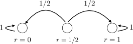
Figure 1: A simple $3$-state Markov reward process.

The benefits of our instance-dependent guarantees are even evident in a model as simple as the $3$-state MRP illustrated in Figure 1. Suppose that we observe noiseless rewards of this MRP and wish to compute its infinite-horizon value function with discount factor $\gamma\in(0,1)$. Bounds based on the contractivity of the Bellman operator [KS99, Kak03, Wai19b] imply that the $\ell_{\infty}$-error of the plug-in estimate scales proportionally to $1/(1-\gamma)^{2}$. The worst-case bounds of Azar et al. [AMK13] imply a rate $1/(1-\gamma)^{3/2}$. But the optimal local result captured in this paper shows that the error is only proportional to $1/(1-\gamma)$. For a discount factor $\gamma=0.99$, this improves the previous bounds by factors of $100$ and $10$, respectively, and consequently, the respective sample complexities by factors of $10^{4}$ and $10^{2}$. Instance-dependent results therefore allow us to differentiate problems that are “solvable” with finite samples from those that are not.

Notation:

For a positive integer $n$, let $[n]:\,=\{1,2,\ldots,n\}$. For a finite set $S$, we use $|S|$ to denote its cardinality. We use $c,C,c_{1},c_{2},\dots$ to denote universal constants that may change from line to line. We use the convenient shorthand $a\lor b:\,=\max\{a,b\}$ and $a\land b=\min\{a,b\}$. We let ${\bf 1}$ denote the all-ones vector in ^D, and abusing notation slightly, we let ${\mathbf{1}\left\{\mathcal{E}\right\}}$ denote the indicator of an event $\mathcal{E}$. Let $e_{j}$ denote the $j$th standard basis vector in ^D. We let $v_{(i)}$ denote the $i$-th order statistic of a vector $v$, i.e., the $i$-th largest entry of $v$. For a pair of vectors $(u,v)$ of compatible dimensions, we use the notation $u\preceq v$ to indicate that the difference vector $v-u$ is entry-wise non-negative. The relation $u\succeq v$ is defined analogously. We let $|u|$ denote the entry-wise absolute value of a vector $u\in^{D}$; squares and square-roots of vectors are, analogously, taken entrywise. Note that for a positive scalar $\lambda$, the statements $|u|\preceq\lambda\cdot{\bf 1}$ and $\|u\|_{\infty}\leq\lambda$ are equivalent. Finally, we let $\|\mathbf{M}\|_{1,\infty}$ denote the maximum $\ell_{1}$-norm of the rows of a matrix $\mathbf{M}$, and refer to it as the $(1,\infty)$-operator norm of a matrix.

2 Background and Problem Formulation

In this section, we introduce the basic notation required to specify a Markov reward process, and formally define the problem of estimating value functions in the generative setting.

2.1 Markov reward processes and value functions

We study Markov reward processes defined on a finite set $\mathcal{X}$ of states, indexed as $\mathcal{X}=\{1,2,\ldots,D\}$. The state evolution over time is determined by a set of transition functions $\{P(\;\cdot\;\mid x),\;\;x\in\mathcal{X}\big{\}}$, with the transition from state $x$ to the next state being randomly chosen according to the distribution $P(\,\cdot\,\mid x)$. For notational convenience, we let $\mathbf{P}\in[0,1]^{D\times D}$ denote a row stochastic (Markov) transition matrix, where row $j$ of this matrix—which we denote by $p_{j}$—collects the transition function of the $j$-th state. Also associated with an MRP is a population reward function $r:\mathcal{X}\mapsto$: transitioning from state $x$ results in the reward $r(x)$. For convenience, we engage in a minor abuse of notation by letting $r$ also denote a vector of length $D$, with $r_{j}$ corresponding to the reward obtained at the $j$-th state.

In this paper, we consider the infinite-horizon, discounted reward as our notion for the long-term value of a state in the MRP. In particular, for a scalar discount factor $\gamma\in(0,1)$, the long-term value of state $x$ in the MRP is given by

$$\theta^{*}(x):\,={\mathbb{E}}\left[\sum_{k=0}^{\infty}\gamma^{k}r(x_{k})\;\;\Big{|}\;\;x_{0}=x\right],\qquad\text{ where }x_{k}\sim P(\;\cdot\;|\;x_{k-1})\text{ for all }k\geq 1.$$

In words, this measures the expected discounted reward obtained by starting at the state $x$, where the expectation is taken with respect to the random transitions over states. Once again, we use $\theta^{*}$ to also denote a vector of length $D$, where $\theta^{*}_{j}$ corresponds to the value of the $j$-th state.

A note to the reader: in the sequel, we often reference a state simply by its index, and often refer to the state space $\mathcal{X}\equiv[D]$. Accordingly, we also use $P(\;\cdot\;\mid j)$ to denote the transition function corresponding to state $j\in[D]$.

2.2 Observation model

Given access to the true transition and reward functions, it is straightforward, at least in principle, to compute the value function. By definition, it is the unique solution of the Bellman fixed point relation

$$\theta^{*}=r+\gamma\mathbf{P}\theta^{*}.$$ (1)

In the learning setting, the pair $(\mathbf{P},r)$ is unknown, and we instead assume access to a black box that generates samples from the transition and reward functions. In this paper, we operate under a setting known as the synchronous or generative setting; it is a stylized observation model that has been used extensively in the study of Markov decision processes (see Kearns and Singh [KS99] for an introduction). Let us introduce it in the context of MRPs: for a given sample index $k=1,2,\ldots,N$ and for each state $j\in[D]$, we observe a random next state $X_{k,j}\in[D]$ drawn according to the transition function $P(\;\cdot\;\mid\;j)$, and a random reward $R_{k,j}$ drawn from a conditional distribution $\mathcal{D}_{r}(\,\cdot\,\mid j)$. Throughout, we assume that the rewards are generated independently across states, with ${\mathbb{E}}[R_{k,j}]=r_{j}$. Letting $\rho(r)$ denote a non-negative vector indexed by the states $j\in[D]$, we assume the conditional distributions $\{\mathcal{D}_{r}(\,\cdot\,\mid j),\;j\in[D]\}$ are $\rho(r)$-sub-Gaussian, meaning that for each $j\in[D]$, we have

$${\mathbb{E}}_{R\sim\mathcal{D}_{r}(\,\cdot\,\mid j)}\Big{[}e^{\lambda(R-r_{j})}\Big{]}\leq e^{\frac{\lambda^{2}\rho_{j}^{2}(r)}{2}}\qquad\mbox{for all $\lambda\in$.}$$ (2)

With $N$ such i.i.d. samples in hand, our goal is to estimate the value function $\theta^{*}$ in the $\ell_{\infty}$-error metric.

Such a goal is particularly relevant to the policy evaluation problem described in the introduction, since $\ell_{\infty}$-estimates of the value function can be used in conjunction with a policy improvement sub-routine to eventually arrive at an optimal policy (see, e.g., Section 1.2.2. of the recent monograph [AJK19]). We note in passing that bounds proved under the generative model may be translated into the more challenging online setting via the notion of Markov cover times (see, e.g., the papers [EDM03, AMGK11] for conversions of this type for Markov decision processes).

3 Main results

We now turn to the statement and discussion of our main results. We begin by providing $\ell_{\infty}$-guarantees on value function estimation for the natural plug-in approach.

3.1 Guarantees for the plug-in approach

A natural approach to this problem is use the observations to construct estimates $(\widehat{\mathbf{P}},\widehat{r})$ of the pair $(\mathbf{P},r)$, and then substitute or “plug in” these estimates into the Bellman equation, thereby obtaining the value function of the MRP having transition matrix $\widehat{\mathbf{P}}$ and reward vector $\widehat{r}$.

In order to define the plug-in estimator, let us introduce some helpful notation. For each time index $k$, we use the associated set of state samples $\{X_{k,j},j\in[D]\}$ to form a random binary matrix $\mathbf{Z}_{k}\in\{0,1\}^{D\times D}$, in which row $j$ has a single non-zero entry, determined by the sample $X_{k,j}$. Thus, the location of the non-zero entry in row $j$ is drawn from the probability distribution defined by $p_{j}$, the $j$-th row of $\mathbf{P}$. Recall that our observations also include the stochastic reward vectors $\{R_{k}\}_{k=1}^{N}$ sampled from the reward distribution $\mathcal{D}_{r}$. Based on these observations, we define the sample means

$$\widehat{\mathbf{P}}=\frac{1}{N}\sum_{k=1}^{N}\mathbf{Z}_{k}\quad\text{ and }\quad\widehat{r}=\frac{1}{N}\sum_{k=1}^{N}R_{k},$$ (3)

which can be seen as unbiased estimates of the transition matrix $\mathbf{P}$ and the reward vector $r$, respectively.

The estimates $(\widehat{\mathbf{P}},\widehat{r})$ define a new MRP, and its value function is given by the fixed point relation

$$\widehat{\theta}_{\mathsf{plug}}=\widehat{r}+\gamma\widehat{\mathbf{P}}\widehat{\theta}_{\mathsf{plug}}.$$ (4)

Solving this fixed point equation, we obtain the closed form expression $\widehat{\theta}_{\mathsf{plug}}=(\mathbf{I}-\gamma\widehat{\mathbf{P}})^{-1}\widehat{r}$ for the plug-in estimator. Note that the terminology “plug-in” arises the fact that $\widehat{\theta}_{\mathsf{plug}}$ is obtained by substituting the estimates $(\widehat{\mathbf{P}},\widehat{r})$ into the original Bellman equation (1). We also note that in this special case—that is, the tabular setting without function approximation—the plug-in estimate is equivalent to the LSTD solution [BB96, Boy02].

In order to establish guarantees for the estimator $\widehat{\theta}_{\mathsf{plug}}$, we require some additional notation. As mentioned before, we are interested in non-asymptotic, instance-dependent guarantees of two types: the first is a bound that can be evaluated in practice from the observed data, and the second is a guarantee that depends on the unknown population quantities $\mathbf{P}$ and $r$. For each vector $\theta\in^{D}$, define the vector of empirical variances

$$\widehat{\sigma}^{2}(\theta) =\widehat{\mathbb{E}}\left|(\mathbf{Z}-\widehat{\mathbf{P}})\theta\right|^{2},$$

where $\widehat{\mathbb{E}}$ denotes expectation over the empirical distribution (i.e., the random matrix $\mathbf{Z}$ is drawn uniformly at random from the set $\{\mathbf{Z}_{k}\}_{k=1}^{N}$). Note that given $\theta$, this quantity is computable purely from the observed samples. On the other hand, the population result will involve the population variance vector

$$\sigma^{2}(\theta) =\mathbb{E}\left|(\mathbf{Z}-\mathbf{P})\theta\right|^{2},$$

where in this case $\mathbf{Z}$ is drawn according to the population model $\mathbf{P}$. As a final definition, the span semi-norm of a value function $\theta$ is given by

$$\|\theta\|_{\operatorname{span}}:\,=\max_{x\in\mathcal{X}}\theta(x)-\min_{x\in\mathcal{X}}\theta(x).$$

Equivalently, the span semi-norm is equal to the variation of the vector $\theta\in^{D}$; see Puterman [Put05] for more details.

We now ready to state our main result for the plug-in estimator.

Theorem 1.

There is a pair of universal constants $(c_{1},c_{2})$ such that if $N\geq c_{1}\frac{\gamma^{2}}{(1-\gamma)^{2}}\log(8D/\delta)$, then each of the following statements holds with probability at least $1-\delta$.

1. We have

   $$\|\widehat{\theta}_{\mathsf{plug}}-\theta^{*}\|_{\infty} \leq c_{2}\left\{\sqrt{\frac{\log(8D/\delta)}{N}}\left(\gamma\|(\mathbf{I}-\gamma\widehat{\mathbf{P}})^{-1}\widehat{\sigma}(\widehat{\theta}_{\mathsf{plug}})\|_{\infty}+\frac{\|\rho(r)\|_{\infty}}{1-\gamma}\right)+\frac{\log(8D/\delta)}{N}\cdot\frac{\gamma\|\widehat{\theta}_{\mathsf{plug}}\|_{\operatorname{span}}}{1-\gamma}\right\}.$$ (5a)

2. We have

   $$\|\widehat{\theta}_{\mathsf{plug}}-\theta^{*}\|_{\infty} \leq c_{2}\left\{\sqrt{\frac{\log(8D/\delta)}{N}}\left(\gamma\left\|(\mathbf{I}-\gamma\mathbf{P})^{-1}\sigma(\theta^{*})\right\|_{\infty}+\frac{\|\rho(r)\|_{\infty}}{1-\gamma}\right)+\frac{\log(8D/\delta)}{N}\cdot\frac{\gamma\|\theta^{*}\|_{\operatorname{span}}}{1-\gamma}\right\}.$$ (5b)

It is worth making a few comments on this theorem, which provides two instance-dependent upper bounds on the error of the plug-in approach. Assuming for simplicity of discussion that the maximum noise reward parameter $\|\rho(r)\|_{\infty}$ is known, then part (a) of the theorem provides a bound that can be evaluated based on the observed data; bounds of this form are especially useful in downstream analyses. For instance, a central consideration in policy iteration methods is to obtain “good enough” value function estimates $\widehat{\theta}$ for fixed policies, in that we have $\|\widehat{\theta}-\theta^{*}\|_{\infty}\leq\epsilon$ for some prescribed tolerance $\epsilon$. Theorem 1(a) provides a method by which such a bound may be verified for the plug-in approach: compute the statistic on the RHS of bound (5a); if this is less than $\epsilon$, then the bound $\|\widehat{\theta}_{\mathsf{plug}}-\theta^{*}\|_{\infty}\leq\epsilon$ holds with probability exceeding $1-\delta$.

On the other hand, Theorem 1(b) provides a guarantee that depends on the unknown problem instance. From the perspective of the analysis, this is the more difficult bound to establish, since it requires a leave-one-out technique to decouple dependencies between the estimate $\widehat{\theta}_{\mathsf{plug}}$ and the matrix $\widehat{\mathbf{P}}$. We expect our technique—presented in full in Section 5.2—and its variants to be more broadly useful in analyzing other problems in reinforcement learning besides the policy evaluation problem considered here.

Third, note that our lower bound on the sample size—which evaluates to $N\geq\frac{c_{1}}{(1-\gamma)^{2}}\log(8D/\delta)$ for any strictly positive discount factor—is unavoidable in general. In particular, for any fixed reward-noise parameter $\|\rho(r)\|_{\infty}>0$, this condition is required in order to obtain a consistent estimate of the value function. On the other hand, in the special case of deterministic rewards ($\|\rho(r)\|_{\infty}=0$), we suspect that this condition can be weakened, but leave this for future work.

Finally, it is worth noting that there are two terms in the bounds of Theorem 1: the first term corresponds to a notion of standard deviations of the estimated/true value function and reward, and the second depends on the span semi-norm of the value function. Are both of these terms necessary? What is the optimal rate at which any value function can be estimated? These questions motivate the analysis to be presented in the following section.

3.2 Is the plug-in approach optimal?

In order to study the question of optimality, we adopt the notion of local minimax risk, in which the performance of an estimator is measured in a worst-case sense locally over natural subsets of the parameter space. Our upper bounds depend on the problem instance via the standard deviation function $\sigma(\theta^{*})$, the reward standard deviation $\rho(r)$, and the span semi-norm of $\theta^{*}$. Accordingly, we define the following subsets of Markov reward processes (MRPs):

$$\mathfrak{M}_{\mathsf{var}}(\vartheta,\varrho) :\,=\Big{\{}\mbox{set of all MRPs s.t. $\|\sigma(\theta^{*})\|_{\infty}\leq\vartheta$ and $\|\rho(r)\|_{\infty}\leq\varrho$}\Big{\}},$$ (6a)

$$\mathfrak{M}_{\mathsf{vfun}}(\zeta,\varrho) :\,=\Big{\{}\mbox{set of all MRPs s.t. $\|\theta^{*}\|_{\operatorname{span}}\leq\zeta$ and $\|\rho(r)\|_{\infty}\leq\varrho$}\Big{\}},\qquad\mbox{and}$$ (6b)

$$\mathfrak{M}_{\mathsf{rew}}(r_{\max},\varrho) :\,=\Big{\{}\mbox{set of all MRPs s.t. $\|r\|_{\infty}\leq r_{\max}$ and $\|\rho(r)\|_{\infty}\leq\varrho$}\Big{\}}.$$ (6c)

Letting $\mathfrak{M}$ be any one of these sets, we use the shorthand $\theta\in\mathfrak{M}$ to mean that $\theta$ is the value function of some MRP in the set $\mathfrak{M}$. Each choice of the set $\mathfrak{M}$ defines the local minimax risk given by

$$\inf_{\widehat{\theta}}\;\sup_{\theta^{*}\in\mathfrak{M}}\;{\mathbb{E}}\left[\|\widehat{\theta}-\theta^{*}\|_{\infty}\right],$$

where the infimum ranges over all measurable functions $\widehat{\theta}$ of $N$ observations from the generative model. With this set-up, we can now state some lower bounds in terms of such local minimax risks:

Theorem 2.

There is a pair of absolute constants $(c_{1},c_{2})$ such that for all $\gamma\in[\tfrac{1}{2},1)$ and sample sizes $N\geq\frac{c_{1}}{1-\gamma}\log(D/2)$, the following statements hold.

1. For each triple of positive scalars $(\vartheta,\zeta,\varrho)$ satisfying $\vartheta\leq\zeta\sqrt{1-\gamma}$, we have

   $$\inf_{\widehat{\theta}}\;\sup_{\theta^{*}\in\mathfrak{M}_{\operatorname{var}}(\vartheta,\varrho)\cap\mathfrak{M}_{\mathsf{vfun}}(\zeta,\varrho)}\;{\mathbb{E}}\left[\|\widehat{\theta}-\theta^{*}\|_{\infty}\right]\geq\frac{c_{2}}{1-\gamma}\sqrt{\frac{\log(D/2)}{N}}\left(\vartheta+\varrho\right).$$ (7a)

2. For each pair of positive scalars $(r_{\max},\varrho)$ satisfying $r_{\max}\geq\varrho\sqrt{\frac{\log D}{N}}$, we have

   $$\inf_{\widehat{\theta}}\;\sup_{\theta^{*}\in\mathfrak{M}_{\mathsf{rew}}(r_{\max},\varrho)}\;{\mathbb{E}}\left[\|\widehat{\theta}-\theta^{*}\|_{\infty}\right]\geq\frac{c_{2}}{1-\gamma}\sqrt{\frac{\log(D/2)}{N}}\left(\frac{r_{\max}}{(1-\gamma)^{1/2}}+\varrho\right).$$ (7b)

Equipped with these lower bounds, we can now assess the local minimax optimality of the plug-in estimator. In order to facilitate this comparison, let us state a corollary of Theorem 1 that provides bounds on the worst-case error of the plug-in estimator over particular subsets of the parameter space. In order to further simplify the comparison, we restrict our attention to the range $\gamma\in[\tfrac{1}{2},1)$ covered by the lower bounds.

Corollary 1.

There are absolute constants $(c_{3},c_{4})$ such that for all $\gamma\in[\tfrac{1}{2},1)$ and sample sizes $N\geq\frac{c_{3}}{(1-\gamma)^{2}}\log(8D/\delta)$, the following statements hold.

1. Consider a triple of positive scalars $(\vartheta,\zeta,\varrho)$ such that $\vartheta\leq\zeta$. Then for any value function $\theta^{*}\in\mathfrak{M}_{\mathsf{var}}(\vartheta,\varrho)\cap\mathfrak{M}_{\mathsf{vfun}}(\zeta,\varrho)$, we have

   $$\|\widehat{\theta}_{\mathsf{plug}}-\theta^{*}\|_{\infty} \leq\frac{c_{4}}{1-\gamma}\left\{\sqrt{\frac{\log(8D/\delta)}{N}}\left(\vartheta+\varrho\right)+\frac{\log(8D/\delta)}{N}\cdot\zeta\right\}$$ (8a)

   with probability at least $$1-\delta$$.

2. Consider an arbitrary pair of positive scalars $(r_{\max},\varrho)$. Then for any value function $\theta^{*}\in\mathfrak{M}_{\mathsf{rew}}(r_{\max},\varrho)$, we have

   $$\|\widehat{\theta}_{\mathsf{plug}}-\theta^{*}\|_{\infty} \leq\frac{c_{4}}{1-\gamma}\sqrt{\frac{\log(8D/\delta)}{N}}\left(\frac{r_{\max}}{(1-\gamma)^{1/2}}+\varrho\right)$$ (8b)

   with probability at least $1-\delta$.

By comparing Corollary 1(b) with Theorem 2(b), we see that the plug-in estimator is minimax optimal (up to constant factors) over the class $\mathfrak{M}_{\mathsf{rew}}(r_{\max},\varrho)$. This conclusion parallels that of Azar et al. [AMK13] for the related problem of optimal state-value function estimation in MDPs. (In our notation, their work applies to the special case of $\varrho=0$, but their analysis can easily be extended to this more general setting.)

A comparison of part (a) of the two results is more interesting. Here we see that the first term in the upper bound (8a) matches the lower bound (7a) up to a constant factor. The second term of inequality (8a), however, does not have an analogous component in the lower bound, and this leads us to the interesting question of whether the analysis of the plug-in estimator can be sharpened so as to remove the dependence of the error on the span semi-norm $\|\theta^{*}\|_{\operatorname{span}}$. Proposition 1, presented in Appendix A, shows that this is impossible in general, and that there are MRPs in which the $\ell_{\infty}$ error can be lower bounded by a term that is proportional to the span semi-norm.

This raises another natural question: Is there a different estimator whose error can be bounded independently of the span semi-norm $\|\theta^{*}\|_{\operatorname{span}}$, and which is able achieve the lower bound (7a)? In the next section, we introduce such an estimator via a median-of-means device.

3.3 Closing the gap via the median-of-means method

In many situations, the span semi-norm of a value function $\theta^{*}$ may be much larger its variance $\sigma(\theta^{*})$ under the transition model. Such a discrepancy arises when there are states with extremely large positive (or negative) rewards that are visited with very low probability. In such cases, the second terms in the bounds (5) dominate the first. It is thus of interest to derive bounds that are purely “variance-dependent” and independent of the span norm. In order to do so, we analyze a slight variant of the plug-in approach. In particular, we analyze the median-of-means estimator, which is a standard robust alternative to the sample mean in other scenarios [NY83, LL20]. In the context of reinforcement learning, Pazis et al. [PPH16] made use of it for online policy optimization in MDPs.

In our setting, we only employ median-of-means to obtain a better estimate of term depending on the transition matrix; we still use the estimate $\widehat{r}$ defined in equation (3) as our estimate of the reward function. Given the data set $\left\{\mathbf{Z}_{k}\right\}_{k=1}^{N}$ and some vector $\theta\in^{D}$, the median-of-means estimate $\widehat{\mathcal{M}}(\theta)$ of the population expectation $\mathbf{P}\theta$ is given by the following nonlinear operation:

• First, split the data set into $K$ equal parts denoted $\{\mathcal{D}_{1},\ldots,\mathcal{D}_{K}\}$, where each subset $\mathcal{D}_{i}$ has size $m=\lfloor N/K\rfloor$.

• Second, compute the empirical mean $\widehat{\mu}_{i}(\theta):\,=\frac{1}{m}\sum_{k\in\mathcal{D}_{i}}\mathbf{Z}_{k}\theta$ for each $i\in[K]$.

• Finally, return the quantity $\widehat{\mathcal{M}}(\theta):\,=\operatorname{med}(\widehat{\mu}_{1}(\theta),\ldots,\widehat{\mu}_{K}(\theta))$, where the median—defined for convenience as the $\lfloor K/2\rfloor$-th order statistic—is taken entry-wise.

The random operator $\widehat{\mathcal{M}}$ defines the median-of-means empirical Bellman operator, given by

$$\widehat{\mathcal{T}}^{\mathsf{MoM}}_{N}(\theta) :\,=\widehat{r}+\gamma\widehat{\mathcal{M}}(\theta).$$ (9)

As shown in Lemma 6 (see Section 5), this operator is $\gamma$-contractive in the $\ell_{\infty}$-norm. Consequently, it has a unique fixed point, which we term the median-of-means value function estimate, denoted by $\widehat{\theta}_{\mathsf{MoM}}$.

In practice, the estimate $\widehat{\theta}_{\mathsf{MoM}}$ can be found by starting at an arbitrary initialization and repeatedly applying the $\gamma$-contractive operator $\widehat{\mathcal{T}}^{\mathsf{MoM}}_{N}$ until convergence. The following theorem provides a population-based guarantee on the error of this estimator.

Theorem 3.

Suppose that the median-of-means operator $\widehat{\mathcal{M}}$ is constructed with the parameter choice $K=8\log(4D/\delta)$. Then there is a universal constant $c$ such that we have

$$\|\widehat{\theta}_{\mathsf{MoM}}-\theta^{*}\|_{\infty} \leq\frac{c}{1-\gamma}\sqrt{\frac{\log(8D/\delta)}{N}}\Big{(}\gamma\|\sigma(\theta^{*})\|_{\infty}+\|\rho(r)\|_{\infty}\Big{)}$$ (10)

with probability exceeding $1-\delta$.

We have thus achieved our goal of obtaining a purely variance-dependent bound. Indeed, for each pair of positive scalars $(\vartheta,\varrho)$, any value function $\theta^{*}\in\mathfrak{M}_{\operatorname{var}}(\vartheta,\varrho)$, and reward distribution satisfying $\|\rho(r)\|_{\infty}\leq\varrho$, we have

$$\|\widehat{\theta}_{\mathsf{MoM}}-\theta^{*}\|_{\infty}\leq\frac{c}{1-\gamma}\sqrt{\frac{\log(8D/\delta)}{N}}\left(\vartheta+\varrho\right),$$

with probability exceeding $1-\delta$. Integrating this tail bound yields an analogous upper bound on the expected error, which matches the lower bound (7a) on the expected error up to a constant factor. As a corollary, we conclude that the minimax risk over the class $\mathfrak{M}_{\operatorname{var}}(\vartheta,\varrho)$ scales as

$$\inf_{\widehat{\theta}}\;\sup_{\theta^{*}\in\mathfrak{M}_{\operatorname{var}}(\vartheta,\varrho)}\;{\mathbb{E}}\left[\|\widehat{\theta}-\theta^{*}\|_{\infty}\right]\asymp\frac{1}{1-\gamma}\sqrt{\frac{\log(D)}{N}}\left(\vartheta+\varrho\right),$$ (11)

and is achieved (up to constant factors) by the estimator $\widehat{\theta}_{\mathsf{MoM}}$.

However, our results fall short of showing that the estimator $\widehat{\theta}_{\mathsf{MoM}}$ is minimax optimal over the class $\mathfrak{M}_{\mathsf{rew}}(r_{\max},\varrho)$ of MRPs with bounded rewards. Indeed, for any value function $\theta^{*}$ in the class $\mathfrak{M}_{\mathsf{rew}}(r_{\max},\varrho)$, Theorem 3 yields the corollary

$$\|\widehat{\theta}_{\mathsf{MoM}}-\theta^{*}\|_{\infty}\leq\frac{c}{1-\gamma}\sqrt{\frac{\log(8D/\delta)}{N}}\left(\gamma\frac{r_{\max}}{1-\gamma}+\varrho\right)$$

with probability exceeding $1-\delta$. Comparing inequality (7b) with this bound, we see that our upper bound on the median-of-means estimator is sub-optimal by a factor $(1-\gamma)^{-\tfrac{1}{2}}$ in the discount complexity. From a technical standpoint, this is due to the fact that our upper bound in Theorem 3 involves the functional $\frac{1}{1-\gamma}\|\sigma(\theta^{*})\|_{\infty}$ and not the sharper functional $\|(\mathbf{I}-\gamma\mathbf{P})^{-1}\sigma(\theta^{*})\|_{\infty}$ present in Theorem 1(b). We believe that this gap is not intrinsic to the MoM method, and conjecture that an upper bound depending on the latter functional can be proved for the estimator $\widehat{\theta}_{\mathsf{MoM}}$; this would guarantee that the median-of-means estimator is also minimax optimal over the class $\mathfrak{M}_{\mathsf{rew}}(r_{\max},\varrho)$.

4 Numerical experiments

In this section, we explore the sharpness of our theoretical predictions, for both the plug-in and the median-of-means (MoM) estimator. Our bounds predict a range of behaviors depending on the scaling of the maximum standard deviation $\|\sigma(\theta^{*})\|_{\infty}$, and the span semi-norm (for the plug-in estimator). Let us verify these scalings via some simple experiments.

4.1 Behavior on the “hard” example used for the lower bound

First, we use a simple variant of our lower bound construction illustrated in panel (a) of Figure 2. This MRP consists of $D=2$ states, where state $1$ stays fixed with probability $p$, transitions to state $2$ with probability $1-p$, and state $2$ is absorbing. The rewards in states $1$ and $2$ are given by $\nu$ and $\nu\tau$, respectively. Here the triple $(p,\nu,\tau)$, along with the discount factor $\gamma$, are parameters of the construction.

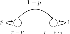
(a)		(b)

Figure 2: (a) Illustration of the MRP $\mathcal{R}_{\mathbf{0}}(p,\nu,\tau)$ used in the simulation, and also as a building block in the lower bound construction of Theorem 2. For the simulation, we choose $p=\tfrac{4\gamma-1}{3\gamma}$, let $\nu=1$, and set $\tau=1-(1-\gamma)^{\alpha}$. (b) Log-log plot of the $\ell_{\infty}$-error versus the discount complexity parameter $1/(1-\gamma)$ for both the plug-in estimator (in $+$ markers) and median-of-means estimator (in $\bullet$ markers) averaged over $T=1000$ trials with $N=10^{4}$ samples each. We have also plotted the least-squares fits through these points, and the slopes of these lines are provided in the legend. In particular, the legend contains the tuple of slopes $(\widehat{\beta}_{\mbox{\tiny{plug}}},\widehat{\beta}_{\mbox{\tiny{MoM}}},\beta^{*})$ for each value of $\alpha$. Logarithms are to the natural base.

In order to parameterize this MRP in a scalarized manner, we vary the triple $(p,\nu,\tau)$ in the following way. First, we fix a scalar $\alpha$ in the unit interval $[0,1]$, and then we set

$$p=\tfrac{4\gamma-1}{3\gamma},\qquad\nu=1,\quad\text{ and }\quad\;\tau=1-(1-\gamma)^{\alpha}.$$

Note that this sub-family of MRPs is fully parameterized by the pair $(\gamma,\alpha)$. Let us clarify why this particular scalarization is interesting. As shown in the proof of Theorem 2 (see equation (34)), the underlying MRP has maximal standard deviation scaling as

$$\|\sigma(\theta^{*})\|_{\infty}\sim\left(\frac{1}{1-\gamma}\right)^{0.5-\alpha}.$$

Consequently, by the bound (10) from Theorem 3, for a fixed sample size $N$, the MoM estimator should have $\ell_{\infty}$-norm scaling as $\left(\frac{1}{1-\gamma}\right)^{1.5-\alpha}$. As we discuss in Appendix B, the same prediction also holds for the plug-in estimator, assuming that $N\succsim\frac{1}{(1-\gamma)}$.

In order to test this prediction, we fixed the parameter $\alpha\in[0,1]$, and generated a range of MRPs with different values of the discount factor $\gamma$. For each such MRP, we drew $N=10^{4}$ samples from the generative observation model and computed both the plug-in and median-of-means estimators, where the latter estimator was run with the choice $K=20$. While the plug-in estimator has a simple closed-form expression, the MoM estimator was obtained by running the median-of-means Bellman operator $\widehat{\mathcal{T}}_{N}^{\mathsf{MoM}}$ iteratively until it converged to its fixed point; we declared that convergence had occurred when the $\ell_{\infty}$-norm of the difference between successive iterates fell below $10^{-8}$.

In panel (b) of Figure 2, we plot the $\ell_{\infty}$-error, of both the plug-in approach as well as the median-of-means estimator, as a function of $\gamma$. The plot shows the behavior for three distinct values $\alpha=\{0,0.5,1\}$. Each point on each curve is obtained by averaging $1000$ Monte Carlo trials of the experiment. Note that on this log-log plot, we see a linear relationship between the log $\ell_{\infty}$-error and log discount complexity, with the slopes depending on the value of $\alpha$. More precisely, from our calculations above, our theory predicts that the log $\ell_{\infty}$-error should be related to the log complexity $\log\big{(}\tfrac{1}{1-\gamma}\big{)}$ in a linear fashion with slope

$$\beta^{*} =1.5-\alpha.$$

Consequently, for both the plug-in and MoM estimators, we performed a linear regression to estimate these slopes, denoted by $\widehat{\beta}_{\mbox{\tiny{plug}}}$ and $\widehat{\beta}_{\mbox{\tiny{MoM}}}$ respectively. The plot legend reports the triple $(\widehat{\beta}_{\mbox{\tiny{plug}}},\widehat{\beta}_{\mbox{\tiny{MoM}}},\beta^{*})$, and for each we see good agreement between the theoretical prediction $\beta^{*}$ and its empirical counterparts.

4.2 When does the MoM estimator perform better than plug-in?

Our theoretical results predict that the MoM estimator should outperform the plug-in approach when the span semi-norm of the value function $\|\theta^{*}\|_{\operatorname{span}}$ is much larger than its maximum standard deviation $\|\sigma(\theta^{*})\|_{\infty}$. Indeed, Proposition 1 in Appendix A demonstrates that there are MRPs on which the $\ell_{\infty}$-error of the plug-in estimator grows with the span semi-norm of the optimal value function. Let us now simulate the behavior of both the plug-in and MoM approach on this MRP, constructed by taking $D/3$ copies of the $3$-state MRP in Figure 3(a).

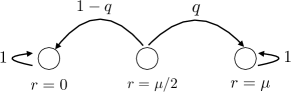
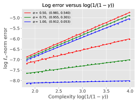
(a)		(b)

Figure 3: (a) Illustration of the MRP $\mathcal{R}_{\mathbf{1}}(q,\mu)$. In the simulation as well as in the lower bound construction of Proposition 1, we concatenate $D/3$ such MRPs to produce an MRP on $D$ states. For the simulation, we choose $D=3\Big{\lfloor}\left(\frac{1}{1-\gamma}\right)^{\alpha}\Big{\rfloor}$ and set $q=\frac{10}{ND}$ and $\mu=1$. (b) Log-log plot of the $\ell_{\infty}$-error versus the discount complexity parameter $1/(1-\gamma)$ for both the plug-in estimator (in $+$ markers) and median-of-means estimator (in $\bullet$ markers) averaged over $T=1000$ trials with $N=10^{4}$ samples each. We have also plotted the least-squares fits through these points, and the slopes of these lines are provided in the legend. In particular, the legend contains the tuple of slopes $(\widehat{\beta}_{\mbox{\tiny{plug}}},\widehat{\beta}_{\mbox{\tiny{MoM}}})$ for each value of $\alpha$. Logarithms are to the natural base.

Our simulation is carried out on $N=10^{4}$ samples from this $D$-state MRP, with noiseless observations of the reward. In order to parameterize the MRP via the discount factor alone, we fix the pair $(q,D)$ in the following way. First, we fix a scalar $\alpha$ in the unit interval $[0,1]$, and then set

$$D=3\Big{\lfloor}\left(\frac{1}{1-\gamma}\right)^{\alpha}\Big{\rfloor}\quad\text{ and }\quad\;q=\frac{10}{ND}.$$

Note that this sub-family of MRPs is fully parameterized by the pair $(\gamma,\alpha)$. The construction also ensures that

$$\frac{\|\theta^{*}\|_{\infty}}{N}\gg\frac{\|\sigma(\theta^{*})\|_{\infty}}{\sqrt{N}},$$ (12)

for this chosen parameterization, and furthermore, that the ratio of the LHS and RHS of inequality (12) increases as the dimension $D$ increases (see the proof of Proposition 1).

As shown in Proposition 1 in Appendix A, the $\ell_{\infty}$ error of the plug-in estimator for this family of MRPs can be lower bounded by $\|\theta^{*}\|_{\infty}/N$. It is also straightforward to show that the error of the MoM estimator is upper bounded by the quantity $\frac{\|\sigma(\theta^{*})\|_{\infty}}{\sqrt{N}}$. Now increasing the value of $\alpha$ increases the dimension $D$, and so the MoM estimator should behave better and better for larger values of $\alpha$. In particular, this behavior can be captured in the log-log plot of the error against $1/(1-\gamma)$, which is presented in Figure 3(b).

The plot shows the behavior for three distinct values $\alpha=\{0.5,0.75,1\}$. Each point on each curve is obtained by averaging $1000$ Monte Carlo trials of the experiment. As expected, the MoM estimator consistently outperforms the plug-in estimator for each value of $\alpha$. Moreover, on this log-log plot, we see a linear relationship between the log $\ell_{\infty}$-error and log discount complexity, with the slopes depending on the value of $\alpha$. For both the plug-in and MoM estimators, we performed a linear regression to estimate these slopes, denoted by $\widehat{\beta}_{\mbox{\tiny{plug}}}$ and $\widehat{\beta}_{\mbox{\tiny{MoM}}}$ respectively. The plot legend reports the pair $(\widehat{\beta}_{\mbox{\tiny{plug}}},\widehat{\beta}_{\mbox{\tiny{MoM}}})$, and we see that the gap between the slopes increases as $\alpha$ increases.

5 Proofs

We now turn to the proofs of our main results. Throughout our proofs, the reader should recall that the values of absolute constants may change from line-to-line. We also use the following facts repeatedly. First, for a row stochastic matrix $\mathbf{M}$ with non-negative entries and any scalar $\gamma\in[0,1)$, we have the infinite series

$$(\mathbf{I}-\gamma\mathbf{M})^{-1}=\sum_{t=0}^{\infty}(\gamma\mathbf{M})^{t},$$ (13a)

which implies that the entries of $$(\mathbf{I}-\gamma\mathbf{M})^{-1} \|(\mathbf{I}-\gamma\mathbf{M})^{-1}\|_{1,\infty}\leq\frac{1}{1-\gamma} \mathbf{A} v$$ are all non-negative. Second, for any such matrix, we also have the bound . Finally, for any matrix with positive entries and a vector of compatible dimension, we have the elementwise inequality

$$|\mathbf{A}v|\preceq\mathbf{A}|v|.$$ (13b)

5.1 Proof of Theorem 1, part (a)

Throughout this proof, we adopt the convenient shorthand $\widehat{\theta}\equiv\widehat{\theta}_{\mathsf{plug}}$ for notational convenience. By the Bellman equations (1) and (4) for $\theta^{*}$ and $\widehat{\theta}$, respectively, we have

$$\widehat{\theta}-\theta^{*} =\gamma\left\{\widehat{\mathbf{P}}\widehat{\theta}-\mathbf{P}\theta^{*}\right\}+(\widehat{r}-r)\;=\;\gamma\widehat{\mathbf{P}}(\widehat{\theta}-\theta^{*})+\gamma(\widehat{\mathbf{P}}-\mathbf{P})\theta^{*}+(\widehat{r}-r).$$

Introducing the shorthand $\widehat{\Delta}:\,=\widehat{\theta}-\theta^{*}$ and re-arranging implies the relation

$$\widehat{\Delta} =\gamma(\mathbf{I}-\gamma\widehat{\mathbf{P}})^{-1}(\widehat{\mathbf{P}}-\mathbf{P})\theta^{*}+(\mathbf{I}-\gamma\widehat{\mathbf{P}})^{-1}(\widehat{r}-r),$$ (14)

and consequently, the elementwise inequality

$$|\widehat{\Delta}| \preceq\gamma(\mathbf{I}-\gamma\widehat{\mathbf{P}})^{-1}|(\widehat{\mathbf{P}}-\mathbf{P})\theta^{*}|+(\mathbf{I}-\gamma\widehat{\mathbf{P}})^{-1}|(\widehat{r}-r)|,$$ (15)

where we have used the relation (13b) with the matrix $\mathbf{A}=(\mathbf{I}-\gamma\widehat{\mathbf{P}})^{-1}$. Given the sub-Gaussian condition on the stochastic rewards, we can apply Hoeffding’s inequality combined with the union bound to obtain the elementwise inequality $|\widehat{r}-r|\preceq c\sqrt{\frac{\log(8D/\delta)}{N}}\cdot\rho(r)$, which holds with probability at least $1-\tfrac{\delta}{4}$. Since the matrix $(\mathbf{I}-\gamma\widehat{\mathbf{P}})^{-1}$ has non-negative entries and $(1,\infty)$-norm at most $\tfrac{1}{1-\gamma}$, we have

$$(\mathbf{I}-\gamma\widehat{\mathbf{P}})^{-1}|\widehat{r}-r| \preceq\frac{c}{1-\gamma}\|\rho(r)\|_{\infty}\sqrt{\frac{\log(8D/\delta)}{N}}{\bf 1}.$$ (16a)

with the same probability. On the other hand, by Bernstein’s inequality, we have

$$|(\widehat{\mathbf{P}}-\mathbf{P})\theta^{*}|\preceq c\Bigg{\{}\sqrt{\frac{\log(8D/\delta)}{N}}\;\cdot\;\sigma(\theta^{*})+\|\theta^{*}\|_{\operatorname{span}}\frac{\log(8D/\delta)}{N}\cdot{\bf 1}\Bigg{\}}$$

with probability at least $$1-\tfrac{\delta}{4}$$, and hence

$$(\mathbf{I}-\gamma\widehat{\mathbf{P}})^{-1}|(\widehat{\mathbf{P}}-\mathbf{P})\theta^{*}| \preceq c\Bigg{\{}\sqrt{\frac{\log(8D/\delta)}{N}}\;\cdot\;\|(\mathbf{I}-\gamma\widehat{\mathbf{P}})^{-1}\sigma(\theta^{*})\|_{\infty}+\frac{\|\theta^{*}\|_{\operatorname{span}}}{1-\gamma}\frac{\log(8D/\delta)}{N}\Bigg{\}}\cdot{\bf 1}.$$ (16b)

Substituting the bounds (16a) and (16b) into the elementwise inequality (15), we find that

$$|\widehat{\Delta}| \preceq c\Bigg{\{}\sqrt{\frac{\log(8D/\delta)}{N}}\;\cdot\;\left(\gamma\|(\mathbf{I}-\gamma\widehat{\mathbf{P}})^{-1}\sigma(\theta^{*})\|_{\infty}+\frac{\|\rho(r)\|_{\infty}}{1-\gamma}\right)+\frac{\gamma\|\theta^{*}\|_{\operatorname{span}}}{1-\gamma}\frac{\log(8D/\delta)}{N}\Bigg{\}}\cdot{\bf 1}$$ (17)

with probability at least $1-\tfrac{\delta}{2}$.

Our next step is to relate the pair of population quantities $(\sigma(\theta^{*}),\|\theta^{*}\|_{\operatorname{span}})$ to their empirical analogues $(\widehat{\sigma}(\widehat{\theta}),\|\widehat{\theta}\|_{\operatorname{span}})$. The following lemma provides such a bound.

Lemma 1 (Population to empirical variance).

We have the element-wise inequality

$$\sigma(\theta^{*}) \preceq 2\widehat{\sigma}(\widehat{\theta})+2|\widehat{\Delta}|+c^{\prime}\|\theta^{*}\|_{\operatorname{span}}\sqrt{\frac{\log(8D/\delta)}{N}}\cdot{\bf 1}$$ (18)

with probability at least $1-\delta/2$.

Taking this lemma as given for the moment, let us complete the proof.

Since the matrix $(\mathbf{I}-\gamma\widehat{\mathbf{P}})^{-1}$ has non-negative entries, we can multiply both sides of the elementwise inequality (18) by it; doing so and taking the $\ell_{\infty}$-norm yields

$$\|(\mathbf{I}-\gamma\widehat{\mathbf{P}})^{-1}\sigma(\theta^{*})\|_{\infty} \leq 2\|(\mathbf{I}-\gamma\widehat{\mathbf{P}})^{-1}\widehat{\sigma}(\widehat{\theta})\|_{\infty}+\frac{2\|\widehat{\Delta}\|_{\infty}}{1-\gamma}+\frac{c^{\prime}\|\theta^{*}\|_{\operatorname{span}}}{1-\gamma}\sqrt{\frac{\log(8D/\delta)}{N}}.$$

Substituting back into the elementwise inequality (17) and taking $\ell_{\infty}$-norms of both sides, we find that

$$\|\widehat{\Delta}\|_{\infty}\leq c\Bigg{\{}\sqrt{\frac{\log(8D/\delta)}{N}}\left(\gamma\|(\mathbf{I}-\gamma\widehat{\mathbf{P}})^{-1}\widehat{\sigma}(\widehat{\theta})\|_{\infty}+\frac{\|\rho(r)\|_{\infty}}{1-\gamma}\right)+\frac{\gamma\|\theta^{*}\|_{\operatorname{span}}}{1-\gamma}\frac{\log(8D/\delta)}{N}\Bigg{\}}\\ +\frac{2c\gamma}{1-\gamma}\sqrt{\frac{\log(8D/\delta)}{N}}\|\widehat{\Delta}\|_{\infty}.$$

Since the span semi-norm satisfies the triangle inequality, we have

$$\|\theta^{*}\|_{\operatorname{span}}\leq\|\widehat{\theta}\|_{\operatorname{span}}+\|\widehat{\Delta}\|_{\operatorname{span}}\leq\|\widehat{\theta}\|_{\operatorname{span}}+2\|\widehat{\Delta}\|_{\infty}.$$

Substituting this bound and re-arranging yields

$$\kappa\|\widehat{\theta}-\theta^{*}\|_{\infty} \leq c\Bigg{\{}\sqrt{\frac{\log(8D/\delta)}{N}}\left(\gamma\|(\mathbf{I}-\gamma\widehat{\mathbf{P}})^{-1}\widehat{\sigma}(\widehat{\theta})\|_{\infty}+\frac{\|\rho(r)\|_{\infty}}{1-\gamma}\right)+\frac{\gamma\|\widehat{\theta}\|_{\operatorname{span}}}{1-\gamma}\frac{\log(8D/\delta)}{N}\Bigg{\}}.$$

where we have introduced the shorthand $\kappa:\,=1-\frac{2c\gamma}{1-\gamma}\left(\sqrt{\frac{\log(8D/\delta)}{N}}+\frac{\log(8D/\delta)}{N}\right)$. Finally, by choosing the pre-factor $c_{1}$ in the lower bound $N\geq c_{1}\gamma^{2}\frac{\log(8D/\delta)}{(1-\gamma)^{2}}$ large enough, we can ensure that $\kappa\geq\frac{1}{2}$, thereby completing the proof of Theorem 1(a).

5.1.1 Proof of Lemma 1

We now turn to the proof of the auxiliary result in Lemma 1. We begin by noting that the statement is trivially true when $N\leq\log(8D/\delta)$, since we have

$$\sigma(\theta^{*})\preceq\|\theta^{*}\|_{\operatorname{span}}{\bf 1}.$$

Thus, by adjusting the constant factors in the statement of the lemma, it suffices to prove the lemma under the assumption $N\geq c\log(8D/\delta)$ for a sufficiently large absolute constant $c$. Accordingly, we make this assumption for the rest of the proof.

We use the following convenient notation for expectations. Let $\mathbb{E}$ denote the vector expectation operator, with the convention that $\mathbb{E}[v]=\mathbf{P}v$. Similarly, let $\widehat{\mathbb{E}}$ denote the vector empirical expectation operator, given by $\widehat{\mathbb{E}}[v]=\widehat{\mathbf{P}}v$. These operators are applied elementwise by definition, and we let $\mathbb{E}_{i}$ and $\widehat{\mathbb{E}}_{i}$ denote the $i$-th entry of each operator, respectively.

With this notation, we have

$$\sigma^{2}(\theta^{*}) =\mathbb{E}\left|\theta^{*}-\mathbb{E}[\theta^{*}]\right|^{2}$$

$$=(\mathbb{E}-\widehat{\mathbb{E}})\Big{|}\theta^{*}-\mathbb{E}[\theta^{*}]\Big{|}^{2}+\widehat{\mathbb{E}}\left|\theta^{*}-\mathbb{E}[\theta^{*}]\right|^{2}$$

$$\preceq(\mathbb{E}-\widehat{\mathbb{E}})\Big{|}\theta^{*}-\mathbb{E}[\theta^{*}]\Big{|}^{2}+2\left|\widehat{\mathbb{E}}[\theta^{*}]-\mathbb{E}[\theta^{*}]\right|^{2}+2\widehat{\mathbb{E}}\left|\theta^{*}-\widehat{\mathbb{E}}[\theta^{*}]\right|^{2}$$

$$=\underbrace{(\mathbb{E}-\widehat{\mathbb{E}})\Big{|}\theta^{*}-\mathbb{E}[\theta^{*}]\Big{|}^{2}}_{T_{1}}+\underbrace{2\left|\widehat{\mathbb{E}}[\theta^{*}]-\mathbb{E}[\theta^{*}]\right|^{2}}_{T_{2}}+2\widehat{\sigma}^{2}(\theta^{*}).$$ (19)

We claim that the terms $T_{1}$ and $T_{2}$ are bounded as follows:

$$T_{1} \preceq\frac{\sigma^{2}(\theta^{*})}{4}+c\|\theta^{*}\|_{\operatorname{span}}^{2}\frac{\log(8D/\delta)}{N}\cdot{\bf 1},\quad\mbox{and}$$ (20a)

$$T_{2} \preceq c\left\{\frac{\log(8D/\delta)}{N}\cdot\sigma^{2}(\theta^{*})+\left(\|\theta^{*}\|_{\operatorname{span}}\frac{\log(8D/\delta)}{N}\right)^{2}\cdot{\bf 1}\right\},$$ (20b)

where each bound holds with probability at least $1-\frac{\delta}{4}$. Taking these bounds as given for the moment, as long as $N\geq c^{\prime}\log(8D/\delta)$ for a sufficiently large constant $c^{\prime}$, we can ensure that

$$T_{1}+T_{2} \preceq\frac{\sigma^{2}(\theta^{*})}{2}+c\|\theta^{*}\|_{\operatorname{span}}^{2}\frac{\log(8D/\delta)}{N}\cdot{\bf 1},$$

Substituting back into our earlier bound (19), we find that

$$\frac{\sigma^{2}(\theta^{*})}{2} \preceq 2\widehat{\sigma}^{2}(\theta^{*})+c^{\prime}\|\theta^{*}\|_{\operatorname{span}}^{2}\frac{\log(8D/\delta)}{N}\cdot{\bf 1}.$$

Rearranging and taking square roots entry-wise, we find that

$$\sigma(\theta^{*}) \preceq\sqrt{4\widehat{\sigma}^{2}(\theta^{*})+2c^{\prime}\|\theta^{*}\|_{\operatorname{span}}^{2}\frac{\log(8D/\delta)}{N}\cdot{\bf 1}}\;\preceq\;2\widehat{\sigma}(\theta^{*})+c^{\prime}\|\theta^{*}\|_{\operatorname{span}}\sqrt{\frac{\log(8D/\delta)}{N}}\cdot{\bf 1}.$$

Finally noting that we have the entry-wise inequality $\widehat{\sigma}(\theta^{*})\preceq\widehat{\sigma}(\widehat{\theta})+|\widehat{\theta}-\theta^{*}|$ establishes the claim of Lemma 1.

It remains to prove the bounds (20a) and (20b).

Proof of bound (20a):

For each index $i\in[D]$, define the random variable $Y_{i}:\,=\big{(}\theta^{*}_{J}-\mathbb{E}_{i}[\theta^{*}]\big{)}^{2}$, where $J$ is an index chosen at random from the distribution $p_{i}$. By definition, each random variable $Y_{i}$ is non-negative, and so with ${\mathbb{E}}$ now denoting the regular expectation of a scalar random variable, we have lower tail bound (Proposition 2.14, [Wai19a])

$$\mathbb{P}\left[\mathbb{E}[Y_{i}]-Y_{i}\geq s\right] \leq\exp\left(-\frac{ns^{2}}{2\mathbb{E}[Y_{i}^{2}]}\right)\qquad\mbox{for all $s>0$.}$$

Moreover, we have $Y_{i}\leq\|\theta^{*}\|^{2}_{\operatorname{span}}$ almost surely, from which we obtain

$$\mathbb{E}[Y_{i}^{2}] \leq\|\theta^{*}\|^{2}_{\operatorname{span}}\mathbb{E}_{i}\left[(\theta^{*}-\mathbb{E}[\theta^{*}])^{2}\right]\;=\;\|\theta^{*}\|_{\operatorname{span}}^{2}\sigma_{i}^{2}(\theta^{*}).$$

Putting together the pieces yields the elementwise inequality

$$T_{1} \preceq c\|\theta^{*}\|_{\operatorname{span}}\sqrt{\frac{\log(8D/\delta)}{N}}\cdot\sigma(\theta^{*})\stackrel{{\scriptstyle{\sf(i)}}}{{\preceq}}\;\frac{\sigma^{2}(\theta^{*})}{8}+c^{\prime}\|\theta^{*}\|_{\operatorname{span}}^{2}\frac{\log(8D/\delta)}{N},$$

with probability at least $1-\delta/3$, where in step ${\sf(i)}$, we have used the inequality $2ab\leq\nu a^{2}+\nu^{-1}b^{2}$, which holds for any triple of positive scalars $(a,b,\nu)$.

Proof of the bound (20b):

From Bernstein’s inequality, we have the element-wise bound

$$\Big{|}\widehat{\mathbb{E}}[\theta^{*}]-\mathbb{E}[\theta^{*}]\Big{|} \preceq c\left\{\sqrt{\frac{\log(8D/\delta)}{N}}\cdot\sigma(\theta^{*})+\|\theta^{*}\|_{\operatorname{span}}\frac{\log(8D/\delta)}{N}\cdot{\bf 1}\right\}$$

with probability at least $1-\delta/4$, and hence

$$T_{2} \preceq c\left\{\frac{\log(8D/\delta)}{N}\cdot\sigma^{2}(\theta^{*})+\left(\|\theta^{*}\|_{\operatorname{span}}\frac{\log(8D/\delta)}{N}\right)^{2}\cdot{\bf 1}\right\},$$

as claimed.

5.2 Proof of Theorem 1, part (b)

Once again, we employ the shorthand $\widehat{\theta}\equiv\widehat{\theta}_{\mathsf{plug}}$ for notational convenience, and also the shorthand $\widehat{\Delta}=\widehat{\theta}-\theta^{*}$. Note that it suffices to show the inequality

$${\mathbb{P}}\left\{\|\widehat{\theta}-\theta^{*}\|_{\infty}\geq c\gamma\left\|(\mathbf{I}-\gamma\mathbf{P})^{-1}|(\widehat{\mathbf{P}}-\mathbf{P})\theta^{*}|\right\|_{\infty}+c(1-\gamma)^{-1}\|\widehat{r}-r\|_{\infty}\right\} \leq\frac{\delta}{2},$$ (21)

from which the theorem follows by application of a Bernstein bound to the first term and Hoeffding bound to the second, in a similar fashion to the inequalities (16). We therefore dedicate the rest of the proof to establishing inequality (21).

5.2.1 Proving the bound (21)

We have

$$\widehat{\Delta}=\widehat{\theta}-\theta^{*} =\gamma\widehat{\mathbf{P}}\widehat{\theta}-\gamma\mathbf{P}\theta^{*}+(\widehat{r}-r)=\gamma(\widehat{\mathbf{P}}-\mathbf{P})\widehat{\theta}+\gamma\mathbf{P}\widehat{\Delta}+(\widehat{r}-r),$$

which implies that

$$\widehat{\Delta}-(\mathbf{I}-\gamma\mathbf{P})^{-1}(\widehat{r}-r)=\gamma(\mathbf{I}-\gamma\mathbf{P})^{-1}(\widehat{\mathbf{P}}-\mathbf{P})\widehat{\theta}\;=\;\gamma(\mathbf{I}-\gamma\mathbf{P})^{-1}(\widehat{\mathbf{P}}-\mathbf{P})\widehat{\Delta}+\gamma(\mathbf{I}-\gamma\mathbf{P})^{-1}(\widehat{\mathbf{P}}-\mathbf{P})\theta^{*}.$$ (22)

Since all entries of $(\mathbf{I}-\gamma\mathbf{P})^{-1}$ are non-negative, we have the element-wise inequalities

$$|\widehat{\Delta}| \preceq\gamma(\mathbf{I}-\gamma\mathbf{P})^{-1}|(\widehat{\mathbf{P}}-\mathbf{P})\widehat{\Delta}|+\gamma(\mathbf{I}-\gamma\mathbf{P})^{-1}|(\widehat{\mathbf{P}}-\mathbf{P})\theta^{*}|+(\mathbf{I}-\gamma\mathbf{P})^{-1}|\widehat{r}-r|$$

$$\preceq\gamma(\mathbf{I}-\gamma\mathbf{P})^{-1}|(\widehat{\mathbf{P}}-\mathbf{P})\widehat{\Delta}|+\gamma(\mathbf{I}-\gamma\mathbf{P})^{-1}|(\widehat{\mathbf{P}}-\mathbf{P})\theta^{*}|+\frac{1}{1-\gamma}\|\widehat{r}-r\|_{\infty}\cdot{\bf 1}.$$ (23)

The second and third terms are already in terms of the desired population-level functionals in equation (21). It remains to bound the first term.

Note that the key difficulty here is the fact that the two matrices $\widehat{\mathbf{P}}-\mathbf{P}$ and $\widehat{\Delta}$ are not independent. As a first attempt to address this dependence, one is tempted to use the fact that provided $N$ is large enough, each row of $\widehat{\mathbf{P}}-\mathbf{P}$ has small $\ell_{1}$-norm; for instance, see Weissman et al. [WOS⁺03] for sharp bounds of this type. In particular, this would allow us to work with the entry-wise bounds

$$|(\widehat{\mathbf{P}}-\mathbf{P})\widehat{\Delta}|\preceq\|\widehat{\mathbf{P}}-\mathbf{P}\|_{1,\infty}\|\widehat{\Delta}\|_{\infty}\cdot{\bf 1}\precsim C\sqrt{\frac{D}{N}}\|\widehat{\Delta}\|_{\infty}\cdot{\bf 1},$$

where the final relation hides logarithmic factors in the pair $(D,\delta)$. Proceeding in this fashion, we would then bound each entry in the first term of equation (23) by $\gamma(1-\gamma)^{-1}\sqrt{\frac{D}{N}}\|\widehat{\Delta}\|_{\infty}$; then choosing $N$ large enough such that $\gamma(1-\gamma)^{-1}\sqrt{\frac{D}{N}}\leq 1/2$ suffices to establish bound (21). However, this requires a sample size $N\gtrsim\frac{\gamma^{2}}{(1-\gamma)^{2}}D$, while we wish to obtain the bound (21) with the sample size $N\gtrsim\frac{\gamma^{2}}{(1-\gamma)^{2}}$. This requires a more delicate analysis.

Our analysis instead proceeds entry-by-entry, and uses a leave-one-out sequence to carefully decouple the dependence between $\widehat{\mathbf{P}}-\mathbf{P}$ and $\widehat{\Delta}$. Let us introduce some notation to make this precise. For each $i\in[D]$, recall that we used $\widehat{p}_{i}$ and $p_{i}$ to denote row $i$ of the matrices $\widehat{\mathbf{P}}$ and $\mathbf{P}$, respectively. Let $\widehat{\mathbf{P}}^{(i)}$ denote the $i$-th leave-one-out transition matrix, which is identical to $\widehat{\mathbf{P}}$ except with row $i$ replaced by the population vector $p_{i}$. Let $\widehat{\theta}^{(i)}:\,=(\mathbf{I}-\gamma\widehat{\mathbf{P}}^{(i)})^{-1}r$ be the value function estimate based on $\widehat{\mathbf{P}}^{(i)}$ and the true reward vector $r$, and denote the associated difference vector by $\widehat{\Delta}^{(i)}:\,=\widehat{\theta}^{(i)}-\theta^{*}$.

Now note that we have

$$\left[(\widehat{\mathbf{P}}-\mathbf{P})\widehat{\Delta}\right]_{i}=\langle\widehat{p}_{i}-p_{i},\,\widehat{\Delta}\rangle=\langle\widehat{p}_{i}-p_{i},\,\widehat{\Delta}^{(i)}\rangle+\langle\widehat{p}_{i}-p_{i},\,\widehat{\theta}-\widehat{\theta}^{(i)}\rangle.$$

This decomposition is helpful because, now, the vectors $\widehat{p}_{i}-p_{i}$ and $\widehat{\Delta}^{(i)}$ are independent by construction, so that standard tail bounds can be used on the first term. For the second term, we use the fact that $\widehat{\theta}\approx\widehat{\theta}^{(i)}$, since the latter is obtained by replacing just one row of the estimated transition matrix. Formally, this closeness will be argued by using the matrix inversion formula. We collect these two results in the following lemma.

Lemma 2.

Suppose that the sample size is lower bounded as $N\geq c^{\prime}\gamma^{2}\frac{\log(8D/\delta)}{(1-\gamma)^{2}}$. Then with probability at least $1-\frac{\delta}{2D}$ and for each $i\in[D]$, we have

$$\gamma|\langle\widehat{p}_{i}-p_{i},\,\widehat{\Delta}^{(i)}\rangle| \leq c\left\{\gamma\|\widehat{\Delta}\|_{\infty}\sqrt{\frac{\log(8D/\delta)}{N}}+\gamma\left|\langle\widehat{p}_{i}-p_{i},\,\theta^{*}\rangle\right|+\|r-\widehat{r}\|_{\infty}\right\}\quad\mbox{and}$$ (24a)

$$\gamma|\langle\widehat{p}_{i}-p_{i},\,\widehat{\theta}^{(i)}-\widehat{\theta}\rangle| \leq c\left\{\gamma\|\widehat{\Delta}\|_{\infty}\sqrt{\frac{\log(8D/\delta)}{N}}+\gamma\left|\langle\widehat{p}_{i}-p_{i},\,\theta^{*}\rangle\right|+\|r-\widehat{r}\|_{\infty}\right\}.$$ (24b)

With this lemma in hand, let us complete the proof. Combining the bounds of Lemma 2 with a union bound over all $D$ entries yields the elementwise inequality

$$\gamma\left|(\widehat{\mathbf{P}}-\mathbf{P})\widehat{\Delta}\right| \preceq c\gamma\left|(\widehat{\mathbf{P}}-\mathbf{P})\theta^{*}\right|+c\left\{\gamma\|\widehat{\Delta}\|_{\infty}\sqrt{\frac{\log(8D/\delta)}{N}}+\|\widehat{r}-r\|_{\infty}\right\}\mathbf{1}$$

with probability at least $1-\delta/2$. Since the entries of $(\mathbf{I}-\gamma\mathbf{P})^{-1}$ are non-negative, we can multiply both sides of this inequality by it, thereby obtaining

$$\gamma(\mathbf{I}-\gamma\mathbf{P})^{-1}\left|(\widehat{\mathbf{P}}-\mathbf{P})\widehat{\Delta}\right| \preceq c\gamma(\mathbf{I}-\gamma\mathbf{P})^{-1}\left|(\widehat{\mathbf{P}}-\mathbf{P})\theta^{*}\right|+\frac{c}{1-\gamma}\left\{\gamma\|\widehat{\Delta}\|_{\infty}\sqrt{\frac{\log(8D/\delta)}{N}}+\|\widehat{r}-r\|_{\infty}\right\}{\bf 1}.$$

Returning to the upper bound (23), we have shown that

$$\|\widehat{\Delta}\|_{\infty} \leq c\gamma\frac{\|\widehat{\Delta}\|_{\infty}}{1-\gamma}\sqrt{\frac{\log(8D/\delta)}{N}}+c^{\prime}\gamma\left\|(\mathbf{I}-\gamma\mathbf{P})^{-1}|(\widehat{\mathbf{P}}-\mathbf{P})\theta^{*}|\right\|_{\infty}+\frac{c}{1-\gamma}\|r-\widehat{r}\|_{\infty}.$$

Under the assumed lower bound on the sample size $N\geq c^{\prime}\gamma^{2}\frac{\log(8D/\delta)}{(1-\gamma)^{2}}$, this inequality implies that

$$\|\widehat{\Delta}\|_{\infty} \leq c^{\prime}\gamma\left\|(\mathbf{I}-\gamma\mathbf{P})^{-1}|(\widehat{\mathbf{P}}-\mathbf{P})\theta^{*}|\right\|_{\infty}+\frac{c}{1-\gamma}\|r-\widehat{r}\|_{\infty},$$

as claimed (21). ∎

We now proceed to a proof of Lemma 2, which uses the following structural lemma relating the quantities $\widehat{\Delta}^{(i)}$ and $\widehat{\Delta}$.

Lemma 3.

Suppose that the sample size is lower bounded as $N\geq c^{\prime}\gamma^{2}\frac{\log(8D/\delta)}{(1-\gamma)^{2}}$. Then with probability at least $1-\frac{\delta}{4D}$ and for each $i\in[D]$, we have

$$\|\widehat{\Delta}^{(i)}\|_{\infty} \leq c\|\widehat{\Delta}\|_{\infty}+\frac{c}{1-\gamma}\Big{\{}\gamma\left|\langle\widehat{p}_{i}-p_{i},\,\theta^{*}\rangle\right|+\|\widehat{r}-r\|_{\infty}\Big{\}}.$$ (25)

This lemma is proved in Section 5.2.3 to follow.

5.2.2 Proof of Lemma 2

We prove the two bounds in turn.

Proof of inequality (24a):

Note that $\widehat{p}_{i}-p_{i}$ and $\widehat{\Delta}^{(i)}$ are independent by construction, so that the Hoeffding inequality yields

$$|\langle\widehat{p}_{i}-p_{i},\,\widehat{\Delta}^{(i)}\rangle| \leq c\|\widehat{\Delta}^{(i)}\|_{\infty}\sqrt{\frac{\log(8D/\delta)}{N}}$$ (26)

with probability at least $1-\delta/(4D)$.

Using this in conjunction with inequality (25) from Lemma 3 yields the bound

$$\gamma|\langle\widehat{p}_{i}-p_{i},\,\widehat{\Delta}^{(i)}\rangle| \leq c\gamma\|\widehat{\Delta}\|_{\infty}\sqrt{\frac{\log(8D/\delta)}{N}}+\frac{c\gamma}{1-\gamma}\sqrt{\frac{\log(8D/\delta)}{N}}\Big{\{}\gamma\left|\langle\widehat{p}_{i}-p_{i},\,\theta^{*}\rangle\right|+\|\widehat{r}-r\|_{\infty}\Big{\}}$$

$$\stackrel{{\scriptstyle{\sf(i)}}}{{\leq}}c\gamma\|\widehat{\Delta}\|_{\infty}\sqrt{\frac{\log(8D/\delta)}{N}}+c\gamma\left|\langle\widehat{p}_{i}-p_{i},\,\theta^{*}\rangle\right|+c\|\widehat{r}-r\|_{\infty},$$

where in step ${\sf(i)}$, we have used the lower bound on the sample size $N\geq c^{\prime}\frac{\gamma^{2}}{(1-\gamma)^{2}}\log(8D/\delta)$.

Proof of inequality (24b):

The proof of this claim is more involved. Using the relation (22) (with suitable modifications of terms), we have

$$\widehat{\theta}^{(i)}-\widehat{\theta} =\gamma(\mathbf{I}-\gamma\widehat{\mathbf{P}})^{-1}(\widehat{\mathbf{P}}^{(i)}-\widehat{\mathbf{P}})\widehat{\theta}^{(i)}+(\mathbf{I}-\gamma\widehat{\mathbf{P}})^{-1}(r-\widehat{r})$$

$$=-\gamma(\mathbf{I}-\gamma\widehat{\mathbf{P}})^{-1}e_{i}\left(\langle\widehat{p}_{i}-p_{i},\,\widehat{\theta}^{(i)}\rangle\right)+(\mathbf{I}-\gamma\widehat{\mathbf{P}})^{-1}(r-\widehat{r}).$$ (27)

Moreover, the Woodbury matrix identity [HJ85] yields

$$\mathbf{M}:\,=\Big{(}\mathbf{I}-\gamma\widehat{\mathbf{P}}\Big{)}^{-1}-\Big{(}\mathbf{I}-\gamma\widehat{\mathbf{P}}^{(i)}\Big{)}^{-1} =-\gamma\frac{(\mathbf{I}-\gamma\widehat{\mathbf{P}}^{(i)})^{-1}e_{i}(\widehat{p}_{i}-p_{i})^{T}(\mathbf{I}-\gamma\widehat{\mathbf{P}}^{(i)})^{-1}}{1-\gamma(\widehat{p}_{i}-p_{i})^{T}(\mathbf{I}-\gamma\widehat{\mathbf{P}}^{(i)})^{-1}e_{i}}.$$

Consequently,

$$\langle\widehat{p}_{i}-p_{i},\,\widehat{\theta}^{(i)}-\widehat{\theta}\rangle =-\gamma(\widehat{p}_{i}-p_{i})^{\top}(\mathbf{I}-\gamma\widehat{\mathbf{P}})^{-1}e_{i}\left(\langle\widehat{p}_{i}-p_{i},\,\widehat{\theta}^{(i)}\rangle\right)+(\widehat{p}_{i}-p_{i})^{\top}(\mathbf{I}-\gamma\widehat{\mathbf{P}})^{-1}(r-\widehat{r})$$

$$=-\gamma(\widehat{p}_{i}-p_{i})^{\top}(\mathbf{I}-\gamma\widehat{\mathbf{P}}^{(i)})^{-1}e_{i}\left(\langle\widehat{p}_{i}-p_{i},\,\widehat{\theta}^{(i)}\rangle\right)+(\widehat{p}_{i}-p_{i})^{\top}(\mathbf{I}-\gamma\widehat{\mathbf{P}}^{(i)})^{-1}(r-\widehat{r})$$

$$\qquad-\gamma(\widehat{p}_{i}-p_{i})^{\top}\mathbf{M}e_{i}\left(\langle\widehat{p}_{i}-p_{i},\,\widehat{\theta}^{(i)}\rangle\right)+(\widehat{p}_{i}-p_{i})^{\top}\mathbf{M}(r-\widehat{r})$$

$$=\left(\langle\widehat{p}_{i}-p_{i},\,\widehat{\theta}^{(i)}\rangle\right)\cdot\frac{2Z^{2}_{i}-Z_{i}}{1-Z_{i}}+T_{i}\cdot\frac{1-2Z_{i}}{1-Z_{i}},$$ (28)

where we have defined, for convenience, the random variables

$$Z_{i}:\,=\gamma(\widehat{p}_{i}-p_{i})^{\top}(\mathbf{I}-\gamma\widehat{\mathbf{P}}^{(i)})^{-1}e_{i}\quad\text{ and }\quad T_{i}:\,=(\widehat{p}_{i}-p_{i})^{\top}(\mathbf{I}-\gamma\widehat{\mathbf{P}}^{(i)})^{-1}(r-\widehat{r}).$$

Since $\widehat{p}_{i}-p_{i}$ is independent of the vector $(\mathbf{I}-\gamma\widehat{\mathbf{P}}^{(i)})^{-1}(r-\widehat{r})$, applying the Hoeffding bound yields the inequality

$$|T_{i}|\leq\frac{c}{1-\gamma}\|r-\widehat{r}\|_{\infty}\sqrt{\frac{\log(8D/\delta)}{N}}$$

with probability exceeding $1-\delta/(4D)$.

On the other hand, exploiting independence between the vectors $\widehat{p}_{i}-p_{i}$ and $(\mathbf{I}-\gamma\widehat{\mathbf{P}}^{(i)})^{-1}e_{i}$ and applying the Hoeffding bound, we also have

$$|Z_{i}|\leq\frac{c\gamma}{1-\gamma}\sqrt{\frac{\log(8D/\delta)}{N}}$$

with probability least $1-\delta/(4D)$. Taking $N\geq c^{\prime}\frac{\gamma^{2}}{(1-\gamma)^{2}}\log(8D/\delta)$ for a sufficiently large constant $c^{\prime}$ ensures that $\gamma|T_{i}|\leq\|r-\widehat{r}\|_{\infty}$ and $|Z_{i}|\leq 1/4$, so that with probability exceeding $1-\delta/(2D)$, inequality (28) yields

$$\gamma|\langle\widehat{p}_{i}-p_{i},\,\widehat{\theta}^{(i)}-\widehat{\theta}\rangle| \leq c\left\{\gamma|\langle\widehat{p}_{i}-p_{i},\,\widehat{\theta}^{(i)}\rangle|+\|r-\widehat{r}\|_{\infty}\right\}$$

$$\leq c\left\{\gamma|\langle\widehat{p}_{i}-p_{i},\,\widehat{\Delta}^{(i)}\rangle|+\gamma|\langle\widehat{p}_{i}-p_{i},\,\theta^{*}\rangle|+\|r-\widehat{r}\|_{\infty}\right\}.$$

Finally, applying part (a) of Lemma 2 completes the proof. ∎

5.2.3 Proof of Lemma 3

Recall our leave-one-out matrix $\widehat{\mathbf{P}}^{(i)}$, and the explicit bound (26). We have

$$\left|\langle\widehat{p}_{i}-p_{i},\,\widehat{\theta}^{(i)}\rangle\right| \leq\left|\langle\widehat{p}_{i}-p_{i},\,\widehat{\Delta}^{(i)}\rangle\right|+\left|\langle\widehat{p}_{i}-p_{i},\,\theta^{*}\rangle\right|\;\leq\;c\|\widehat{\Delta}^{(i)}\|_{\infty}\sqrt{\frac{\log(8D/\delta)}{N}}+\left|\langle\widehat{p}_{i}-p_{i},\,\theta^{*}\rangle\right|$$ (29)

with probability at least $1-\delta/(4D)$. Substituting inequality (29) into the bound (5.2.2), we find that

$$\|\widehat{\theta}^{(i)}-\widehat{\theta}\|_{\infty} \leq\frac{c}{1-\gamma}\left\{\gamma\|\widehat{\Delta}^{(i)}\|_{\infty}\cdot\sqrt{\frac{\log(8D/\delta)}{N}}+\gamma\left|\langle\widehat{p}_{i}-p_{i},\,\theta^{*}\rangle\right|+\|r-\widehat{r}\|_{\infty}\right\}.$$ (30)

Finally, the triangle inequality yields

$$\|\widehat{\Delta}^{(i)}\|_{\infty} \leq\|\widehat{\Delta}\|_{\infty}+\|\widehat{\theta}^{(i)}-\widehat{\theta}\|_{\infty}$$

$$\leq\;\|\widehat{\Delta}\|_{\infty}+\frac{c}{1-\gamma}\left\{\gamma\|\widehat{\Delta}^{(i)}\|_{\infty}\cdot\sqrt{\frac{\log(8D/\delta)}{N}}+\gamma\left|\langle\widehat{p}_{i}-p_{i},\,\theta^{*}\rangle\right|+\|r-\widehat{r}\|_{\infty}\right\}.$$

For $N\geq c^{\prime}\gamma^{2}\frac{\log(8D/\delta)}{(1-\gamma)^{2}}$ with $c^{\prime}$ sufficiently large, we have

$$\|\widehat{\Delta}^{(i)}\|_{\infty} \leq c\|\widehat{\Delta}\|_{\infty}+\frac{c}{1-\gamma}\Big{\{}\gamma\left|\langle\widehat{p}_{i}-p_{i},\,\theta^{*}\rangle\right|+\|\widehat{r}-r\|_{\infty}\Big{\}}$$

with probability at least $1-\frac{\delta}{4D}$, which completes the proof of Lemma 3. ∎

Since Corollary 1 follows from Theorem 1, we prove it first before moving to a proof of Theorem 2 in Section 5.4.

5.3 Proof of Corollary 1

In order to prove part (a), consider inequality (14) and further use the fact that $\|(\mathbf{I}-\gamma\widehat{\mathbf{P}})^{-1}\|_{1,\infty}\leq\tfrac{1}{1-\gamma}$ to obtain the element-wise bound

$$|\widehat{\theta}-\theta^{*}| \preceq\frac{\gamma}{1-\gamma}\|(\widehat{\mathbf{P}}-\mathbf{P})\theta^{*}\|_{\infty}{\bf 1}+\frac{\|\widehat{r}-r\|_{\infty}}{1-\gamma}\cdot{\bf 1}.$$

Applying Bernstein’s bound to the first term and Hoeffding’s bound to the second completes the proof.

In order to prove part (b) of the corollary, we apply Lemma 7 of Azar et al. [AMK13]—in particular, equation (17) of that paper. Tailored to this setting, their result leads to the point-wise bound

$$\|(\mathbf{I}-\gamma\mathbf{P})^{-1}\sigma(\theta^{*})\|_{\infty}\leq c\frac{r_{\max}}{(1-\gamma)^{3/2}}.$$

We also have the bound

$$\|\theta^{*}\|_{\operatorname{span}}\leq 2\|\theta^{*}\|_{\infty}=2\|(\mathbf{I}-\gamma\mathbf{P})^{-1}r\|_{\infty}\leq\frac{2r_{\max}}{1-\gamma},$$

so that combining the pieces and applying Theorem 1(b), we obtain

$$\|\widehat{\theta}-\theta^{*}\|_{\infty}\leq\frac{c}{(1-\gamma)}\left\{\sqrt{\frac{\log(8D/\delta)}{N}}\left(\gamma\frac{r_{\max}}{(1-\gamma)^{1/2}}+\|\rho(r)\|_{\infty}\right)+\gamma\cdot\frac{\log(8D/\delta)}{N}\frac{r_{\max}}{1-\gamma}\right\}.$$

Finally, when $N\geq c_{1}\frac{\log(8D/\delta)}{1-\gamma}$ for a sufficiently large constant $c_{1}$, we have

$$\frac{\log(8D/\delta)}{N}\frac{r_{\max}}{1-\gamma}\leq c\sqrt{\frac{\log(8D/\delta)}{N}}\frac{r_{\max}}{(1-\gamma)^{1/2}},$$

thereby establishing the claim. ∎

5.4 Proof of Theorem 2

For all of our lower bounds, we assume that the reward distribution takes the Gaussian form

$$\mathcal{D}_{r}(\,\cdot\,\mid j)=\mathcal{N}(r_{j},\varrho^{2})$$ (31)

for each state $j$. Note that this reward distribution satisfies $\|\rho(r)\|_{\infty}=\varrho$ by construction.

Let us begin with a short overview of our proof, which proceeds in two steps. First, we suppose that the transition matrix $\mathbf{P}$ is known exactly, and the hardness of the estimation problem is due to noisy observations of the reward function. In particular, letting $\mathfrak{M}_{\mathbf{I}}(r_{\max},\varrho)$ denote the class of all MRPs with the specific reward observation model (31), and for which the transition matrix is the identity matrix $\mathbf{I}$ and the rewards are uniformly bounded as $\|r\|_{\infty}\leq r_{\max}$, we show that

$$\inf_{\widehat{\theta}}\sup_{\theta^{*}\in\mathfrak{M}_{\mathbf{I}}(r_{\max},\varrho)}{\mathbb{E}}\|\widehat{\theta}-\theta^{*}\|_{\infty}\geq c\left\{\frac{\varrho}{1-\gamma}\cdot\sqrt{\frac{\log(D)}{N}}\land\frac{r_{\max}}{1-\gamma}\right\}.$$ (32)

Note that for each pair of positive scalars $(\vartheta,r_{\max})$ we have the inclusions

$$\mathfrak{M}_{\mathbf{I}}(r_{\max},\varrho)\subseteq\mathfrak{M}_{\operatorname{var}}(\vartheta,\varrho)\quad\text{ and }\quad\mathfrak{M}_{\mathbf{I}}(r_{\max},\varrho)\subseteq\mathfrak{M}_{\mathsf{rew}}(r_{\max},\varrho),$$

and so that the lower bound (32) carries over to the classes $\mathfrak{M}_{\operatorname{var}}(\vartheta,\varrho)$ and $\mathfrak{M}_{\mathsf{rew}}(r_{\max},\varrho)$.

Next, we suppose that the population reward function $r$ is known exactly ($\varrho=0$), and the hardness of the estimation problem is only due to uncertainty in the transitions. Under this setting, we prove the lower bounds

$$\inf_{\widehat{\theta}}\;\sup_{\theta^{*}\in\mathfrak{M}_{\operatorname{var}}(\vartheta,0)}{\mathbb{E}}\|\widehat{\theta}-\theta^{*}\|_{\infty} \geq c\frac{\vartheta}{1-\gamma}\cdot\sqrt{\frac{\log(D/2)}{N}},\qquad\text{ and }$$ (33a)

$$\inf_{\widehat{\theta}}\;\sup_{\theta^{*}\in\mathfrak{M}_{\mathsf{rew}}(r_{\max},0)}{\mathbb{E}}\|\widehat{\theta}-\theta^{*}\|_{\infty} \geq c\frac{r_{\max}}{(1-\gamma)^{3/2}}\cdot\sqrt{\frac{\log(D/2)}{N}}.$$ (33b)

Since $\mathfrak{M}_{\operatorname{var}}(\vartheta,0)\subset\mathfrak{M}_{\operatorname{var}}(\vartheta,\varrho)$ for any $\varrho>0$, these lower bounds also carry over to the more general setting. The minimax lower bounds of Theorem 2 are obtained by taking the maximum of the bounds (32) and (33). Let us now establish the two previously claimed bounds.

5.4.1 Proof of claim (32)

For some positive scalar $\alpha$ to be chosen shortly, consider $D$ distinct reward vectors $\{r^{(1)},\ldots,r^{(D)}\}$, where the vector $r^{(i)}\in^{D}$ has entries

$$r^{(i)}_{j} :\,=\begin{cases}\alpha&\text{ if }i=j\\ 0&\text{ otherwise,}\end{cases}\qquad\text{ for all }j\in[D].$$

Denote by $\mathcal{R}^{(i)}$ the MRP with reward function $r^{(i)}$; and transition matrix $\mathbf{I}$. Thus, the $i$-th value function is given by the vector $(\theta^{*})^{(i)}:\,=\frac{1}{1-\gamma}r^{(i)}$.

By construction, we have $\|(\theta^{*})^{(i)}-(\theta^{*})^{(j)}\|_{\infty}=\alpha/(1-\gamma)$ for each pair of distinct indices $(i,j)$. Furthermore, the KL divergence between Gaussians of variance $\varrho^{2}$ centered at $r^{(i)}$ and $r^{(j)}$ is given by

$$D_{\mathsf{KL}}\left(\mathcal{N}(r^{(i)},\varrho^{2}\mathbf{I})\;\|\;\mathcal{N}(r^{(j)},\varrho^{2}\mathbf{I})\right)=\frac{\|r^{(i)}-r^{(j)}\|_{2}^{2}}{\varrho^{2}}=\frac{2\alpha^{2}}{\varrho^{2}}.$$

Thus, applying the local packing version of Fano’s method (§15.3.3, [Wai19a]), we have

$$\inf_{\widehat{\theta}}\;\sup_{\theta^{*}\in\{\mathfrak{M}^{(i)}\}_{i\in[D]}}{\mathbb{E}}\|\widehat{\theta}-\theta^{*}\|_{\infty}\geq c\frac{\alpha}{1-\gamma}\left(1-\frac{2\frac{\alpha^{2}}{\varrho^{2}}N+\log 2}{\log D}\right).$$

Setting $\alpha=\varrho\sqrt{\frac{\log D}{6N}}\land r_{\max}$ yields the claimed lower bound.

5.4.2 Proof of claim (33)

This lower bound is based on a modification of constructions used by Lattimore and Hutter [LH14] and Azar et al. [AMK13]. Our proof, however, is tailored to the generative observation model.

Our proof is structured as follows. First, we construct a family of “hard” MRPs and prove a minimax lower bound as a function of parameters used to define this family. Constructing this family of hard instances requires us to first define a basic building block: a two-state MRP that was illustrated in Figure 2(a). After obtaining this general lower bound, we then set the scalars that parameterize the hard class MRP appropriately to obtain the two claimed bounds.

We now describe the two-state MRP in more detail. For a pair of parameters $(p,\tau)$, each in the unit interval $[0,1]$, and a positive scalar $\nu$, consider the two-state Markov reward process $\mathcal{R}_{\mathbf{0}}(p,\nu,\tau)$, with transition matrix and reward vector given by

$$\mathbf{P}_{\mathbf{0}}=\begin{bmatrix}p&1-p\\ 0&1\end{bmatrix}\qquad\text{ and }\qquad r_{\mathbf{0}}=\begin{bmatrix}\nu\\ \nu\cdot\tau\end{bmatrix},$$

respectively. See Figure 2 for an illustration of this MRP.

A straightforward calculation yields that it has value function and corresponding standard deviation vector given by

$$\theta^{*}(p,\nu,\tau)=\nu\begin{bmatrix}\frac{1-\gamma+\gamma\tau(1-p)}{(1-\gamma p)(1-\gamma)}\\ \frac{\tau}{1-\gamma}\end{bmatrix}\qquad\text{ and }\qquad\sigma(\theta^{*})=\nu\begin{bmatrix}\frac{(1-\tau)\sqrt{p(1-p)}}{1-\gamma p}\\ 0\end{bmatrix},$$ (34)

respectively, where we have used the shorthand $\theta^{*}\equiv\theta^{*}(p,\nu,\tau)$. We also have $\|\theta^{*}\|_{\operatorname{span}}=\frac{\nu(1-\tau)}{1-\gamma p}$; the two scalars $(\nu,\tau)$ allow us to control the quantities $\|\sigma(\theta^{*})\|_{\infty}$ and $\|\theta^{*}\|_{\operatorname{span}}$. Index the states of this MRP by the set $\{0,1\}$, and consider now a sample drawn from this MRP under the generative model. We see a pair of states drawn according to the respective rows of the transition matrix $\mathbf{P}_{\mathbf{0}}$; the first state is drawn according to the Bernoulli distribution $\mbox{\sf Ber}(p)$, and the second state is deterministic and equal to $1$. For convenience, we use ${\mathbb{P}}(p)=(\mbox{\sf Ber}(p),1)$ to denote the distribution of this pair of states.

Our hard class of instances is based in part on the difficulty of distinguishing two such MRPs that are close in a specific sense. Let us make this intuition precise. For two scalar values $0\leq p_{2}\leq p_{1}\leq 1$, some algebra yields the relation

$$\|\theta^{*}(p_{1},\nu,\tau)-\theta^{*}(p_{2},\nu,\tau)\|_{\infty}=\nu\cdot\frac{(p_{1}-p_{2})(1-\tau)}{(1-\gamma p_{1})(1-\gamma p_{2})}.$$ (35)

In the sequel, we work with the choices

$$p_{1}=\frac{4\gamma-1}{3\gamma}\quad\mbox{and}\quad p_{2}=p_{1}-\frac{1}{8}\sqrt{\frac{p_{1}(1-p_{1})}{N}\log(D/2)},$$

which, under the assumed lower bound on the sample size $N$, are both scalars in the range $\big{[}\tfrac{1}{2},1\big{)}$ for all discount factors $\gamma\in\big{[}\tfrac{1}{2},1\big{)}$. Moreover, it is worth noting the relations

$$1-p_{1} =\frac{1-\gamma}{3\gamma},\quad c_{1}\frac{1-\gamma}{3\gamma}\leq 1-p_{2}\leq c_{2}\frac{1-\gamma}{3\gamma}$$

$$1-\gamma p_{1} =\frac{4}{3}(1-\gamma),\quad\qquad\text{ and }\quad c_{1}(1-\gamma)\leq 1-\gamma p_{2}\leq c_{2}(1-\gamma),$$ (36)

where the inequalities on the right hold provided $N\geq\frac{c\gamma}{1-\gamma}\log(D/2)$ for a sufficiently large constant $c$. Here the pair of constants $(c_{1},c_{2})$ are universal, depend only on $c$, and may change from line to line.

We also require the following lemma, proved in Section 5.4.3 to follow, which provides a useful bound on the KL divergence between ${\mathbb{P}}(p_{1})$ and ${\mathbb{P}}(p_{2})$.

Lemma 4.

For each pair $p,q\in[1/2,1)$, we have

$$D_{\mathsf{KL}}\left({\mathbb{P}}(p)\|{\mathbb{P}}(q)\right)\leq\frac{(p-q)^{2}}{(p\lor q)(1-(p\lor q))}.$$

We are now in a position to describe the hard family of MRPs over which we prove a general lower bound. Suppose that $D$ is even for convenience, and consider a set of $D/2$ “master” MRPs $\bar{\mathfrak{M}}:\,=\{\mathcal{R}_{1},\ldots,\mathcal{R}_{D/2}\}$ each on $D$ states constructed as follows. Decompose each master MRP into $D/2$ sub-MRPs of two states each; index the $k$-th sub-MRP in the $j$-th master MRP by $\mathcal{R}_{j,k}$. For each pair $j,k\in[D/2]$, set

$$\mathcal{R}_{j,k}=\begin{cases}\mathcal{R}_{\mathbf{0}}(p_{1},\nu,\tau)&\text{ if }j\neq k\\ \mathcal{R}_{\mathbf{0}}(p_{2},\nu,\tau)&\text{ otherwise.}\end{cases}$$

Let $\theta^{*}_{j}$ denote the value function corresponding to MRP $\mathcal{R}_{j}$, and let $\mathbb{P}_{j}^{N}$ denote the distribution of state transitions observed from the MRP $\mathcal{R}_{j}$ under the generative model. Also note that for each $i\in[D/2]$, we have

$$\|\sigma(\theta^{*}_{i})\|_{\infty}=\nu\frac{(1-\tau)\sqrt{p_{1}(1-p_{1})}}{(1-\gamma p_{1})}.$$ (37)

Lower bounding the minimax risk over this class:

We again use the local packing form of Fano’s method (§15.3.3, [Wai19a]) to establish a lower bound. Choose some index $J$ uniformly at random from the set $[D/2]$, and suppose that we draw $N$ i.i.d. samples $Y^{N}:\,=(Y_{1},\ldots,Y_{N})$ from the MRP $\mathcal{R}_{J}$ under the generative model. Here each $Y_{i}\in\mathcal{X}^{D}$ represents a random set of $D$ states, and the goal of the estimator is to identify the random index $J$ and, consequently, to estimate the value function $\theta^{*}_{J}$. Let us now lower bound the expected error incurred in this $(D/2)$-ary hypothesis testing problem. Fano’s inequality yields the bound

$$\inf_{\widehat{\theta}}\sup_{\theta^{*}\in\bar{\mathfrak{M}}}{\mathbb{E}}\|\widehat{\theta}-\theta^{*}\|_{\infty}\geq\frac{1}{2}\min_{j\neq k}\;\|\theta^{*}_{j}-\theta^{*}_{k}\|_{\infty}\left(1-\frac{I(J;Y^{N})+\log 2}{\log(D/2)}\right),$$ (38)

where $I(J;Y^{N})$ denotes the mutual information between $J$ and $Y^{N}$.

Let us now bound the two terms that appear in inequality (38). By equation (35), we have

$$\|\theta^{*}_{j}-\theta^{*}_{k}\|_{\infty}=\nu\cdot\frac{(p_{1}-p_{2})(1-\tau)}{(1-\gamma p_{1})(1-\gamma p_{2})}\qquad\text{ for all }1\leq j\neq k\leq D/2.$$

Furthermore, since the samples $Y_{1},\ldots,Y_{N}$ are i.i.d., the chain rule of mutual information yields

$$\frac{1}{N}I(J;Y^{N})=I(J;Y_{1}) \leq\max_{j\neq k}\;D_{\mathsf{KL}}(\mathbb{P}_{j}\|\mathbb{P}_{k})$$

$$\stackrel{{\scriptstyle{\sf(i)}}}{{=}}D_{\mathsf{KL}}({\mathbb{P}}(p_{1})\|{\mathbb{P}}(p_{2}))+D_{\mathsf{KL}}({\mathbb{P}}(p_{2})\|{\mathbb{P}}(p_{1}))$$

$$\stackrel{{\scriptstyle{\sf(ii)}}}{{\leq}}2\frac{(p_{1}-p_{2})^{2}}{p_{1}(1-p_{1})},$$

where step ${\sf(i)}$ is a consequence of the construction, which ensures that the distributions $\mathbb{P}_{j}$ and $\mathbb{P}_{k}$ coincide on all but the $j$-th and $k$-th sub-MRPs. On the other hand, step ${\sf(ii)}$ follows from Lemma 4, and the fact that $p_{2}\leq p_{1}$.

Putting together the pieces, we now have

$$\inf_{\widehat{\theta}}\sup_{\theta^{*}\in\bar{\mathfrak{M}}}{\mathbb{E}}\|\widehat{\theta}-\theta^{*}\|_{\infty}\geq\frac{\nu}{2}\cdot\frac{(p_{1}-p_{2})(1-\tau)}{(1-\gamma p_{1})(1-\gamma p_{2})}\left(1-\frac{2N\frac{(p_{1}-p_{2})^{2}}{p_{1}(1-p_{1})}+\log 2}{\log(D/2)}\right).$$

Recall the choice $p_{1}-p_{2}=\frac{1}{8}\sqrt{\frac{p_{1}(1-p_{1})}{N}\log(D/2)}$. For $D\geq 8$, this ensures, for a small enough positive constant $c$, the bound

$$\inf_{\widehat{\theta}}\sup_{\theta^{*}\in\bar{\mathfrak{M}}}{\mathbb{E}}\|\widehat{\theta}-\theta^{*}\|_{\infty}\geq c\nu\frac{(1-\tau)\sqrt{p_{1}(1-p_{1})}}{(1-\gamma p_{1})}\cdot\sqrt{\frac{\log(D/2)}{N}}\frac{1}{1-\gamma p_{2}}.$$ (39)

With the relation (39) at hand, we now turn to proving the two sub-claims in equation (33).

Proof of claim (33a):

Recall equation (37); for $i\in[D/2]$, we have

$$\|\sigma(\theta^{*}_{i})\|_{\infty}=\nu\frac{(1-\tau)\sqrt{p_{1}(1-p_{1})}}{(1-\gamma p_{1})}\quad\text{ and }\quad\|\theta^{*}_{i}\|_{\operatorname{span}}=\nu\frac{(1-\tau)}{(1-\gamma p_{1})}.$$

Now for every pair of scalars $(\vartheta,\zeta)$ satisfying $\vartheta=\zeta\sqrt{1-\gamma}$, set $\tau=1/2$ and $\nu=2\zeta(1-\gamma p_{1})$. With this choice of parameters, we have the inclusion $\mathfrak{M}_{\operatorname{var}}(\vartheta,0)\cap\mathfrak{M}_{\mathsf{vfun}}(\zeta,0)\subseteq\bar{\mathfrak{M}}$, and evaluating the bound (39) yields

$$\inf_{\widehat{\theta}}\sup_{\theta^{*}\in\mathfrak{M}_{\mathsf{var}}(\vartheta,0)\cap\mathfrak{M}_{\mathsf{vfun}}(\zeta,0)}{\mathbb{E}}\|\widehat{\theta}-\theta^{*}\|_{\infty} \geq c\vartheta\sqrt{\frac{\log(D/2)}{N}}\frac{1}{1-\gamma p_{2}}$$

$$\stackrel{{\scriptstyle{\sf(ii)}}}{{=}}c\vartheta\sqrt{\frac{\log(D/2)}{N}}\frac{1}{1-\gamma},$$

where in step ${\sf(ii)}$, we have used inequality (5.4.2). The same lower bound clearly also extends to the set $\mathfrak{M}_{\mathsf{var}}(\vartheta,0)\cap\mathfrak{M}_{\mathsf{vfun}}(\zeta,0)$ for $\zeta\geq\vartheta(1-\gamma)^{-1/2}$; this establishes part (a) of the theorem.

Proof of claim (33b):

Given a value $r_{\max}$, set $\tau=0$ and $\nu=r_{\max}$ and note that the rewards of all the MRPs in the set $\bar{\mathfrak{M}}$ satisfy $\|r\|_{\infty}\leq\nu$. Hence, we have $\mathfrak{M}_{\mathsf{rew}}(r_{\max},0)\subseteq\bar{\mathfrak{M}}$ for this choice of parameters. Using inequality (39) and recalling the bounds (5.4.2) once again, we have

$$\inf_{\widehat{\theta}}\sup_{\theta^{*}\in\mathfrak{M}_{\mathsf{rew}}(r_{\max},0)}{\mathbb{E}}\|\widehat{\theta}-\theta^{*}\|_{\infty} \geq cr_{\max}\frac{\sqrt{p_{1}(1-p_{1})}}{(1-\gamma p_{1})}\cdot\sqrt{\frac{\log(D/2)}{N}}\frac{1}{1-\gamma p_{2}}$$

$$\geq c\frac{r_{\max}}{(1-\gamma)^{3/2}}\sqrt{\frac{\log(D/2)}{N}}.$$

5.4.3 Proof of Lemma 4

By construction, the second state of the Markov chain is absorbing, so it suffices to consider the KL divergence between the first components of the distributions ${\mathbb{P}}(p)$ and ${\mathbb{P}}(q)$. These are Bernoulli random variables $\mbox{\sf Ber}(p)$ and $\mbox{\sf Ber}(q)$, and the following calculation bounds their KL divergence:

$$D_{\mathsf{KL}}\left(\mbox{\sf Ber}(p)\|\mbox{\sf Ber}(q)\right) =p\log\frac{p}{q}+(1-p)\log\frac{1-p}{1-q}$$

$$\stackrel{{\scriptstyle{\sf(ii)}}}{{\leq}}p\cdot\frac{p-q}{q}+(1-p)\cdot\frac{q-p}{1-q}$$

$$=\frac{(p-q)^{2}}{q(1-q)},$$

where step ${\sf(ii)}$ uses the inequality $\log(1+x)\leq x$, which is valid for all $x>-1$. A similar inequality holds with the roles of $p$ and $q$ reversed, and the denominator of the expression is lower for the larger value $p\lor q$. This completes the proof.

5.5 Proof of Theorem 3

Note that the median-of-means operator is applied elementwise; denote the $i$-th such operator by $\widehat{\mathcal{M}}_{i}$. Let $\widehat{\mathcal{M}}-\mathbf{P}$ denote the elementwise difference of operator $\widehat{\mathcal{M}}$ and the linear operator $\mathbf{P}$; its $i$-th component is given by the operator $\widehat{\mathcal{M}}_{i}(\cdot)-\langle p_{i},\,\cdot\rangle$.

We require two technical lemmas in the proof. The power of the median-of-means device is clarified by the first lemma, which is an adaptation of classical results (see, e.g., [NY83, JVV86]).

Lemma 5.

Suppose that $K=8\log(4D/\delta)$ and $m=\lfloor N/K\rfloor$. Then there is a universal constant $c$ such that for each index $i\in[D]$ and each fixed vector $\theta\in^{D}$, we have

$$\Pr\left\{|(\widehat{\mathcal{M}}_{i}-p_{i})(\theta)|\geq c\;\sigma_{i}(\theta)\sqrt{\frac{\log(8D/\delta)}{N}}\right\}\leq\frac{\delta}{4D}.$$

Comparing this lemma to the Bernstein bound (cf. equation (16b)), we see that we no longer pay in the span semi-norm $\|\theta^{*}\|_{\operatorname{span}}$, and this is what enables us to establish the solely variance-dependent bound (10).

We also require the following lemma that guarantees that the median-of-means Bellman operator is contractive.

Lemma 6.

The median-of-means operator is $1$-Lipschitz in the $\ell_{\infty}$-norm, and satisfies

$$|\widehat{\mathcal{M}}(\theta_{1})-\widehat{\mathcal{M}}(\theta_{2})|\leq\|\theta_{1}-\theta_{2}\|_{\infty}\qquad\text{ for all vectors }\theta_{1},\theta_{2}\in^{D}.$$

Consequently, the empirical operator $\widehat{\mathcal{T}}^{\mathsf{MoM}}_{N}$ is $\gamma$-contractive in $\ell_{\infty}$-norm and satisfies

$$|\widehat{\mathcal{T}}^{\mathsf{MoM}}_{N}(\theta_{1})-\widehat{\mathcal{T}}^{\mathsf{MoM}}_{N}(\theta_{2})|\leq\gamma\|\theta_{1}-\theta_{2}\|_{\infty}\qquad\text{ for all pairs of value functions }(\theta_{1},\theta_{2}).$$

See Section 5.5.1 for the proof of Lemma 6.

We are now in a position to establish the theorem, where we now use the shorthand $\widehat{\theta}\equiv\widehat{\theta}_{\mathsf{MoM}}$ for convenience. Note that the vectors $\theta^{*}$ and $\widehat{\theta}$ satisfy the fixed point relations

$$\theta^{*}=r+\gamma\mathbf{P}\theta^{*},\quad\mbox{and}\quad\widehat{\theta}=\widehat{r}+\gamma\widehat{\mathcal{M}}(\widehat{\theta}),$$

respectively. Taking differences, the error vector $\widehat{\Delta}=\widehat{\theta}-\theta^{*}$ satisfies the relation

$$\widehat{\theta}-\theta^{*} =\gamma(\widehat{\mathcal{M}}(\widehat{\Delta}+\theta^{*})-\mathbf{P}\theta^{*})+\widehat{r}-r$$

$$=\gamma(\widehat{\mathcal{M}}(\widehat{\Delta}+\theta^{*})-\widehat{\mathcal{M}}(\theta^{*}))+\gamma(\widehat{\mathcal{M}}-\mathbf{P})(\theta^{*})+(\widehat{r}-r).$$

Taking $\ell_{\infty}$-norms on both sides and using the triangle inequality, we have

$$\|\widehat{\Delta}\|_{\infty} \leq\gamma\|\widehat{\mathcal{M}}(\theta^{*}+\widehat{\Delta})-\widehat{\mathcal{M}}(\theta^{*})\|_{\infty}+\gamma|(\widehat{\mathcal{M}}-\mathbf{P})(\theta^{*})|+\|\widehat{r}-r\|_{\infty}$$

$$\stackrel{{\scriptstyle{\sf(i)}}}{{\leq}}\gamma\|\widehat{\Delta}\|_{\infty}+\gamma|(\widehat{\mathcal{M}}-\mathbf{P})(\theta^{*})|+\|\widehat{r}-r\|_{\infty},$$

where step ${\sf(i)}$ is a result of Lemma 6. Finally, applying Lemma 5 in conjunction with the Hoeffding inequality and a union bound over all $D$ indices completes the proof.

5.5.1 Proof of Lemma 6

The second claim follows directly from the first by noting that

$$|\widehat{\mathcal{T}}^{\mathsf{MoM}}_{N}(\theta_{1})-\widehat{\mathcal{T}}^{\mathsf{MoM}}_{N}(\theta_{2})|=\gamma|\widehat{\mathcal{M}}(\theta_{1})-\widehat{\mathcal{M}}(\theta_{2})|.$$

In order to prove the first claim, recall that for each $\theta\in^{D}$, we have $\widehat{\mathcal{M}}(\theta)=\operatorname{med}(\widehat{\mu}_{1}(\theta),\ldots,\widehat{\mu}_{K}(\theta))$, where the median—defined as the $\lfloor K/2\rfloor$-th order statistic—is taken entry-wise. By definition, for each $i\in[K]$, we have

$$\|\widehat{\mu}_{i}(\theta_{1})-\widehat{\mu}_{i}(\theta_{2})\|_{\infty} =\left\|\left(\frac{1}{m}\sum_{k\in\mathcal{D}_{i}}\mathbf{Z}_{k}\right)(\theta_{1}-\theta_{2})\right\|_{\infty}$$

$$\leq\left\|\frac{1}{m}\sum_{k\in\mathcal{D}_{i}}\mathbf{Z}_{k}\right\|_{1,\infty}\|\theta_{1}-\theta_{2}\|_{\infty}$$

$$\stackrel{{\scriptstyle{\sf(i)}}}{{=}}\|\theta_{1}-\theta_{2}\|_{\infty},$$

where step ${\sf(i)}$ is a result of the fact that $\frac{1}{m}\sum_{k\in\mathcal{D}_{i}}\mathbf{Z}_{k}$ is a row stochastic matrix with non-negative entries. Finally, we have the entry-wise bound

$$|\widehat{\mathcal{M}}(\theta_{1})-\widehat{\mathcal{M}}(\theta_{2})| =|\operatorname{med}(\widehat{\mu}_{1}(\theta_{1}),\ldots,\widehat{\mu}_{K}(\theta_{1}))-\operatorname{med}(\widehat{\mu}_{1}(\theta_{2}),\ldots,\widehat{\mu}_{K}(\theta_{2}))|$$

$$\stackrel{{\scriptstyle{\sf(ii)}}}{{\preceq}}\|\theta_{1}-\theta_{2}\|_{\infty}\cdot{\bf 1},$$

where step ${\sf(ii)}$ follows from our definition of the median as the $\lfloor K/2\rfloor$-th order statistic, and Lemma 7 to follow. This completes the proof of Lemma 6. ∎

Lemma 7.

For each pair of vectors $(u,v)$ of dimension $D$ and each index $i\in[D]$, we have

$$|u_{(i)}-v_{(i)}|\leq\|u-v\|_{\infty}.$$

Proof.

Assume without loss of generality that the entries of $u$ are sorted in increasing order (so that $u_{1}\leq u_{2}\leq\ldots\leq u_{D}$), and let $w$ denote a vector containing the entries of $v$ sorted in increasing order. We then have

$$|u_{(i)}-v_{(i)}|=|u_{i}-w_{i}|\leq\|u-w\|_{\infty}\stackrel{{\scriptstyle{\sf(i)}}}{{\leq}}\|u-v\|_{\infty},$$

where step ${\sf(i)}$ follows from the rearrangement inequality applied to the $\ell_{\infty}$-norm [Vin90]. ∎

6 Discussion

Our work investigates the local minimax complexity of value function estimation in Markov reward processes. Our upper bounds are instance-dependent, and we also provide minimax lower bounds that hold over natural subsets of the parameter space. The plug-in approach is shown to be optimal over the class of MRPs with bounded rewards, and a variant based on the median-of-means device achieves optimality over the class of MRPs having value functions with bounded variance.

Our results also leave a few interesting technical questions unresolved. Let us start with two inter-related questions: Is Corollary 1(a) sharp, say up to a logarithmic factor in the dimension? Is the median-of-means approach minimax-optimal over the class of MRPs having bounded rewards? We conjecture that both of these questions can be answered in the affirmative, but there are technical challenges to overcome. For instance, while the median-of-means device is crucial to removing the span-norm dependence in Corollary 1(a), it leads to a non-linear update rule that needs to be much more carefully handled in order to ensure minimax optimality.

A second set of technical questions concerns the definition of “locality” in our bounds. Are our results also sharp under alternative local minimax parameterizations (say in terms of the functional $\|(\mathbf{I}-\gamma\mathbf{P})^{-1}\sigma(\theta^{*})\|_{\infty}$)? Is there a more fine-grained lower bound analysis that shows the (sub)-optimality of these approaches, and are there better adaptive procedures for this problem? The literature on estimating functionals of discrete distributions [JVHW15] shows that additional refinements over the plug-in approach are usually beneficial; is that also the case here? There is also the related question of whether a minimax lower bound can be proved over a local neighborhood of every point $\theta^{*}$. We remark that guarantees of this flavor exist in a variety of related problems in both the asymptotic and non-asymptotic settings [vdV00, CL04, ZCDL16]. Indeed, in a follow-up paper [KPR⁺20] with a superset of the current authors, we have shown such a local lower bound for this problem, which is achieved via stochastic approximation coupled with a variance reduction device.

In a complementary direction, another interesting question is to ask how function approximation affects these bounds. Our techniques should be useful in answering some of these questions, and also more broadly in proving analogous guarantees in the more challenging policy optimization setting.

Finally, there is the question of removing our assumption on the generative model: How does the plug-in estimator behave when it is computed on a sampled trajectory of the system? A classical solution is the blocking method of simulating the generative model from such samples [Yu94]: given a sampled trajectory, chop it into pieces of length (roughly) equal to the mixing time of the Markov chain, and to treat the respective first sample from each of these pieces as (approximately) independent. But clearly, this approach is somewhat wasteful, and there have been recent refinements in related problems when the mixing time can become arbitrarily large [SMT⁺18]. It would be interesting to explore these approaches and derive instance-dependent guarantees in the $L^{2}_{\mu}$-norm, where $\mu$ is the stationary distribution of the Markov chain.

Acknowledgements

AP was supported in part by a research fellowship from the Simons Institute for the Theory of Computing. MJW and AP were partially supported by National Science Foundation Grant DMS-1612948 and Office of Naval Research Grant ONR-N00014-18-1-2640.

Appendix A Dependence of plug-in error on span semi-norm

In this section, we state and prove a proposition that provides a family of MRPs in which the $\ell_{\infty}$-error of the plug-in estimator can be completely characterized by the span semi-norm of the optimal value function.

Proposition 1.

Suppose that the rewards are observed noiselessly, with $\rho(r)=0$. There is a pair of universal positive constants $(c_{1},c_{2})$ such that for any triple of positive scalars $(\zeta,N,D)$, there is a $D$-state MRP for which

$$\|\theta^{*}\|_{\infty}=\zeta\quad\text{ and }\quad\frac{\|\sigma(\theta^{*})\|_{\infty}}{N}\leq\frac{3}{\sqrt{D}}\cdot\frac{\zeta}{N},$$ (40)

and for which the error of the plug-in estimator satisfies

$$c_{1}\gamma\frac{\zeta}{N}\quad\stackrel{{\scriptstyle(a)}}{{\leq}}\;{\mathbb{E}}\left[\|\widehat{\theta}_{\mathsf{plug}}-\theta^{*}\|_{\infty}\right]\;\stackrel{{\scriptstyle(b)}}{{\leq}}\;c_{2}\gamma\frac{\zeta\log(1+D/3)}{N}\left\{(\log\log(1+D/3))^{-1}\land 1\right\}.$$ (41)

A few comments are in order. First, note that equation (40) guarantees that we have

$$\frac{1}{\sqrt{N}}\cdot\|(\mathbf{I}-\gamma\mathbf{P})^{-1}\sigma(\theta^{*})\|_{\infty}\lesssim\frac{1}{\sqrt{D}}\frac{1}{(1-\gamma)N}\|\theta^{*}\|_{\operatorname{span}}$$

for large values of the dimension $D$, so that the first term in the guarantee (5b) is dominated by the second. In particular, suppose that $D\gg\frac{1}{(1-\gamma)^{2}}$; then we have

$$\frac{1}{\sqrt{N}}\cdot\|(\mathbf{I}-\gamma\mathbf{P})^{-1}\sigma(\theta^{*})\|_{\infty}\ll\frac{1}{N}\|\theta^{*}\|_{\operatorname{span}}.$$

In other words, if our analysis was loose in that the error of the plug-in estimator depended only on the functional $\frac{1}{\sqrt{N}}\cdot\|(\mathbf{I}-\gamma\mathbf{P})^{-1}\sigma(\theta^{*})\|_{\infty}$, then it would be impossible to prove a lower bound that involves the quantity $\frac{\|\theta^{*}\|_{\operatorname{span}}}{N}$. On the other hand, equation (41) shows that this such a lower bound can indeed be proved: the plug-in error is characterized precisely by the quantity $\gamma\frac{\|\theta^{*}\|_{\operatorname{span}}}{N}$ up to a logarithmic factor in the dimension $D$.

Second, note that while equation (41) shows that the plug-in error must have some span semi-norm dependence, it falls short of showing the stronger lower bound

$$c_{1}\frac{\zeta}{(1-\gamma)N}\leq{\mathbb{E}}\left[\|\widehat{\theta}_{\mathsf{plug}}-\theta^{*}\|_{\infty}\right],$$ (42)

which would show, for instance, that Corollary 1(a) is sharp up to a logarithmic factor. We conjecture that there is an MRP for which the bound (42) holds.

Finally, it is worth commenting on the logarithmic factor that appears in the upper bound of equation (41). Note that for sufficiently large $D$, the logarithmic factor is proportional to $\log D/\log\log D$. This is consequence of applying Bennett’s inequality instead of Bernstein’s inequality, and we conjecture that the same factor ought to replace the factor $\log D$ factor multiplying the span semi-norm in the upper bound (5b).

A.1 Proof of Proposition 1

In order to prove Proposition 1, it suffices to construct an MRP satisfying condition (40) and compute its plug-in estimator in closed form. With this goal in mind, suppose that for simplicity that $D$ is divisible by three, and consider $D/3$ copies of the $3$-state MRP from Figure 3(a). By construction, we have $\|\sigma(\theta^{*})\|_{\infty}=\mu\sqrt{q(1-q)}$, and $\|\theta^{*}\|_{\operatorname{span}}=\frac{\mu}{(1-\gamma)}$. Setting $q=\frac{10}{ND}$, we see that condition (40) is immediately satisfied with $\zeta=\frac{\mu}{(1-\gamma)}$.

It remains to verify the claim (41). Note that the plug-in estimator for this MRP can be computed in closed form. In particular, it is straightforward to verify that for each state $i$ having reward $\mu/2$, we have

$$\frac{N(1-\gamma)}{\gamma\mu}\left(\widehat{\theta}_{\mathsf{plug}}(i)-\theta^{*}_{i}\right)\stackrel{{\scriptstyle d}}{{=}}\mbox{\sf Bin}(N,q)-Nq,$$ (43)

where we have used the notation $\widehat{\theta}_{\mathsf{plug}}(i)$ to denote the $i$-th entry of the vector $\widehat{\theta}_{\mathsf{plug}}$. Furthermore, these $D/3$ random variables are independent. Thus, the (scaled) $\ell_{\infty}$-error of the plug-in estimator is equal to the maximum absolute deviation in a collection of independent binomial random variables.

Proof of inequality (41), part (a):

The following technical lemma provides a lower bound on the deviation of binomials, and its proof is postponed to the end of this section.

Lemma 8.

Let $X_{1},\ldots,X_{k}$ denote independent random variables with distribution $\mbox{\sf Bin}\left(n,\frac{1}{3kn}\right)$. Let $Y_{j}=X_{j}-{\mathbb{E}}[X_{j}]$ for each $1\leq j\leq k$. Then, we have

$${\mathbb{E}}\left[\max_{1\leq j\leq k}|Y_{j}|\right]\geq\frac{4}{9}.$$

Applying Lemma 8 with $k=D/3$ in conjunction with the characterization (43), and substituting our choices of the pair $(\mu,q)$ yields

$${\mathbb{E}}\left[\|\widehat{\theta}_{\mathsf{plug}}-\theta^{*}\|_{\infty}\right]\geq\frac{4}{9}\cdot\frac{\zeta\gamma}{N}.$$

Proof of inequality (41), part (b):

Corollary 3.1(ii) and Lemma 3.3 of Wellner [Wel17] yield, to the best of our knowledge, the sharpest available upper bound on the maximum absolute deviation of $\mbox{\sf Bin}(n,q)$ random variables in the regime $nq(1-q)\ll 1$:

$${\mathbb{E}}\left[\max_{1\leq j\leq k}|Y_{j}|\right]\leq\sqrt{12}\cdot\frac{\log(1+k)}{\log\log(1+k)}\quad\text{ if }\quad\log(1+k)\geq 5.$$ (44)

Combining this bound with the Bernstein bound when $k$ is small, and substituting the various quantities completes the proof.

Proof of Lemma 8:

Employing the shorthand $q=\frac{1}{3kn}$, we have

$${\mathbb{E}}\left[\max_{1\leq j\leq k}|Y_{j}|\right] \geq\left(1-nq\right)\cdot\Pr\left\{\max_{1\leq j\leq k}X_{j}\geq 1\right\}$$

$$=\left(1-nq\right)\cdot(1-(1-q)^{nk})$$

$$\geq\frac{2}{3}\cdot\left(1-\sqrt[3]{\left(1-\frac{1}{3nk}\right)^{3nk}}\right)$$

$$\geq\frac{2}{3}\cdot\left(1-e^{-1/3}\right)\geq\frac{4}{9}.$$

Appendix B Calculations for the “hard” sub-class

Recall from equation (34) our previous calculation of the value function and standard deviation, from which we have

$$\|\sigma(\theta^{*})\|_{\infty}=\nu(1-\tau)\frac{\sqrt{p(1-p)}}{1-\gamma p},\qquad\|(\mathbf{I}-\gamma\mathbf{P})^{-1}\sigma(\theta^{*})\|_{\infty}=\nu(1-\tau)\frac{\sqrt{p(1-p)}}{(1-\gamma p)^{2}},$$

and $\|\theta^{*}\|_{\operatorname{span}}=\nu(1-\tau)\frac{1}{1-\gamma p}$. Substituting in our choices $\nu=1$, $p=\frac{4\gamma-1}{3\gamma}$, and $\tau=1-(1-\gamma)^{\alpha}$ and simplifying by employing inequality (5.4.2), we have

$$\|\sigma(\theta^{*})\|_{\infty}\sim\left(\frac{1}{1-\gamma}\right)^{0.5-\alpha},\;\|(\mathbf{I}-\gamma\mathbf{P})^{-1}\sigma(\theta^{*})\|_{\infty}\sim\left(\frac{1}{1-\gamma}\right)^{1.5-\alpha},\;\text{ and }\;\|\theta^{*}\|_{\operatorname{span}}\sim\left(\frac{1}{1-\gamma}\right)^{1-\alpha},$$

for each discount factor $\gamma\geq\tfrac{1}{2}$. Here, the $\sim$ notation indicates that the LHS can be sandwiched between two terms that are proportional to the RHS such that the factors of proportionality are strictly positive and $\gamma$-independent.

For the plug-in estimator, its performance will be determined by the maximum of the two terms

$$\frac{\|(\mathbf{I}-\gamma\mathbf{P})^{-1}\sigma(\theta^{*})\|_{\infty}}{\sqrt{N}}\sim\frac{1}{\sqrt{N}}\left(\frac{1}{1-\gamma}\right)^{1.5-\alpha}\quad\mbox{and}\quad\frac{\|\theta^{*}\|_{\operatorname{span}}}{(1-\gamma)N}\sim\frac{1}{N}\left(\frac{1}{1-\gamma}\right)^{2-\alpha}.$$

In the regime $N\succsim\frac{1}{1-\gamma}$, the first term will be dominant.

References

- [AJK19] A. Agarwal, N. Jiang, and S. M. Kakade. Reinforcement learning: Theory and algorithms. Technical Report, CS Department, UW Seattle, 2019.
- [AKY20] A. Agarwal, S. M. Kakade, and L. F. Yang. Model-based reinforcement learning with a generative model is minimax optimal. In Conference on Learning Theory, pages 67–83, 2020.
- [AMGK11] M. G. Azar, R. Munos, M. Ghavamzadeh, and H. J. Kappen. Speedy -learning. In Advances in Neural Information Processing Systems, pages 2411–2419, 2011.
- [AMK13] M. G. Azar, R. Munos, and H. J. Kappen. Minimax PAC bounds on the sample complexity of reinforcement learning with a generative model. Machine Learning, 91:325–349, 2013.
- [AOM17] M. G. Azar, I. Osband, and R. Munos. Minimax regret bounds for reinforcement learning. In Proceedings of the International Conference on Machine Learning, 2017.
- [BB96] S. J. Bradtke and A. G. Barto. Linear least-squares algorithms for temporal difference learning. Machine learning, 22(1-3):33–57, 1996.
- [BE02] O. Bousquet and A. Elisseeff. Stability and generalization. Journal of machine learning research, 2(Mar):499–526, 2002.
- [Ber95a] D. P. Bertsekas. Dynamic programming and stochastic control, volume 1. Athena Scientific, Belmont, MA, 1995.
- [Ber95b] D.P. Bertsekas. Dynamic programming and stochastic control, volume 2. Athena Scientific, Belmont, MA, 1995.
- [BGSL08] P. Balakrishna, R. Ganesan, L. Sherry, and B. S. Levy. Estimating taxi-out times with a reinforcement learning algorithm. In Proceedings of the IEEE/AIAA 27th Digital Avionics Systems Conference, pages 3–D. IEEE, 2008.
- [BM00] V. S. Borkar and S. P. Meyn. The ODE method for convergence of stochastic approximation and reinforcement learning. SIAM Journal on Control and Optimization, 38(2):447–469, 2000.
- [BM11] F. Bach and E. Moulines. Non-asymptotic analysis of stochastic optimization algorithms for machine learning. In Advances in neural information processing systems, December 2011.
- [Bor98] V. S. Borkar. Asynchronous stochastic approximations. SIAM Journal on Control and Optimization, 36(3):840–851, 1998.
- [Boy02] J. A. Boyan. Technical update: Least-squares temporal difference learning. Machine learning, 49(2-3):233–246, 2002.
- [BRS18] J. Bhandari, D. Russo, and R. Singal. A finite time analysis of temporal difference learning with linear function approximation. arXiv preprint arXiv:1806.02450, 2018.
- [BT96] D. P. Bertsekas and J. N. Tsitsiklis. Neuro-dynamic programming. Athena Scientific, 1996.
- [CFMW19] Y. Chen, J. Fan, C. Ma, and K. Wang. Spectral method and regularized mle are both optimal for top- ranking. The Annals of Statistics, 47(4):2204–2235, 2019.
- [CL04] T. T. Cai and M. G. Low. An adaptation theory for nonparametric confidence intervals. The Annals of statistics, 32(5):1805–1840, 2004.
- [CMSS20] Z. Chen, S. T. Maguluri, S. Shakkottai, and K. Shanmugam. Finite-sample analysis of stochastic approximation using smooth convex envelopes. arXiv preprint arXiv:2002.00874, 2020.
- [DB15] C. Dann and E. Brunskill. Sample complexity of episodic fixed-horizon reinforcement learning. In Advances in Neural Information Processing Systems, pages 2818–2826, 2015.
- [dlPG12] V. de la Pena and E. Giné. Decoupling: from dependence to independence. Springer Science & Business Media, 2012.
- [DM17] A. M. Devraj and S. P. Meyn. Fastest convergence for Q-learning. arXiv preprint arXiv:1707.03770, 2017.
- [DMR19] T. T. Doan, S. T. Maguluri, and J. Romberg. Finite-time performance of distributed temporal difference learning with linear function approximation. arXiv preprint arXiv:1907.12530, 2019.
- [DNP14] C. Dann, G. Neumann, and J. Peters. Policy evaluation with temporal differences: A survey and comparison. The Journal of Machine Learning Research, 15(1):809–883, 2014.
- [DSTM18] G. Dalal, B. Szörényi, G. Thoppe, and S. Mannor. Finite sample analyses for TD(0) with function approximation. In Thirty-Second AAAI Conference on Artificial Intelligence, 2018.
- [Dur99] R. Durrett. Essentials of stochastic processes, volume 1. Springer, 1999.
- [EDM03] E. Even-Dar and Y. Mansour. Learning rates for -learning. Journal of machine learning research, 5:1–25, 2003.
- [Fel66] W. Feller. An Introduction to Probability Theory and its Applications: Volume II. John Wiley and Sons, New York, 1966.
- [FMP08] J. Frank, S. Mannor, and D. Precup. Reinforcement learning in the presence of rare events. In Proceedings of the International conference on Machine learning, pages 336–343. ACM, 2008.
- [Gos09] A. Gosavi. Reinforcement learning: A tutorial survey and recent advances. INFORMS Journal on Computing, 21(2):178–192, 2009.
- [HJ85] R. A. Horn and C. R. Johnson. Matrix Analysis. Cambridge University Press, Cambridge, 1985.
- [JA18] N. Jiang and A. Agarwal. Open problem: The dependence of sample complexity lower bounds on planning horizon. In Conference On Learning Theory, pages 3395–3398, 2018.
- [JJS94] T. Jaakkola, M. I. Jordan, and S. P. Singh. Convergence of stochastic iterative dynamic programming algorithms. In Advances in neural information processing systems, pages 703–710, 1994.
- [JVHW15] J. Jiao, K. Venkat, Y. Han, and T. Weissman. Minimax estimation of functionals of discrete distributions. IEEE Transactions on Information Theory, 61(5):2835–2885, 2015.
- [JVV86] M. R. Jerrum, L. G. Valiant, and V. V. Vazirani. Random generation of combinatorial structures from a uniform distribution. Theoretical Computer Science, 43:169–188, 1986.
- [Kak03] S. M. Kakade. On the sample complexity of reinforcement learning. PhD thesis, Gatsby Computational Neuroscience Unit, 2003.
- [KPR+20] K. Khamaru, A. Pananjady, F. Ruan, M. J. Wainwright, and M. I. Jordan. Is temporal difference learning optimal? An instance-dependent analysis. arXiv preprint arXiv:2003.07337, 2020.
- [KS99] M. Kearns and S. Singh. Finite-sample convergence rates for -learning and indirect algorithms. In Advances in neural information processing systems, 1999.
- [LH14] T. Lattimore and M. Hutter. Near-optimal PAC bounds for discounted MDPs. Theoretical Computer Science, 558:125–143, 2014.
- [LL20] G. Lecué and M. Lerasle. Robust machine learning by median-of-means: theory and practice. Annals of Statistics, 48(2):906–931, 2020.
- [LS18] C. Lakshminarayanan and C. Szepesvári. Linear stochastic approximation: How far does constant step-size and iterate averaging go? In Proceedings of the International Conference on Artificial Intelligence and Statistics, pages 1347–1355, 2018.
- [MMM14] O.-A. Maillard, T. A. Mann, and S. Mannor. How hard is my MDP? the distribution-norm to the rescue. In Advances in Neural Information Processing Systems, pages 1835–1843, 2014.
- [MWCC18] C. Ma, K. Wang, Y. Chi, and Y. Chen. Implicit regularization in nonconvex statistical estimation: Gradient descent converges linearly for phase retrieval and matrix completion. In Proceedings of the International Conference on Machine Learning, pages 3345–3354, 2018.
- [NJLS09] A. Nemirovski, A. Juditsky, G. Lan, and A. Shapiro. Robust stochastic approximation approach to stochastic programming. SIAM Jour. Opt., 19(4):1574–1609, 2009.
- [NY83] A. S. Nemirovsky and D. B. Yudin. Problem Complexity and Method Efficiency in Optimization. John Wiley and Sons, New York, 1983.
- [PJ92] B. T. Polyak and A. B. Juditsky. Acceleration of stochastic approximation by averaging. SIAM J. Control and Optimization, 30(4):838–855, 1992.
- [PPH16] J. Pazis, R. E. Parr, and J. P. How. Improving PAC exploration using the median of means. In Advances in Neural Information Processing Systems, pages 3898–3906, 2016.
- [Put05] M. L. Puterman. Markov decision processes: Discrete stochastic dynamic programming. Wiley, 2005.
- [SB18] R. S. Sutton and A. G. Barto. Reinforcement Learning: An Introduction. MIT Press, Cambridge, MA, 2nd edition, 2018.
- [SJ19] M. Simchowitz and K. G. Jamieson. Non-asymptotic gap-dependent regret bounds for tabular MDPs. In Advances in Neural Information Processing Systems, pages 1151–1160, 2019.
- [SMT+18] M. Simchowitz, H. Mania, S. Tu, M. I. Jordan, and B. Recht. Learning without mixing: Towards a sharp analysis of linear system identification. In Conference on Learning Theory, pages 439–473, 2018.
- [SSM07] D. Silver, R. S. Sutton, and M. Müller. Reinforcement learning of local shape in the game of Go. In Proceedings of the International Joint Conferences on Artificial Intelligence, volume 7, pages 1053–1058, 2007.
- [Sut88] R. S. Sutton. Learning to predict by the methods of temporal differences. Machine learning, 3(1):9–44, 1988.
- [SWW+18] A. Sidford, M. Wang, X. Wu, L. Yang, and Y. Ye. Near-optimal time and sample complexities for solving Markov decision processes with a generative model. In Advances in Neural Information Processing Systems, 2018.
- [SWWY18] A. Sidford, M. Wang, X. Wu, and Y. Ye. Variance reduced value iteration and faster algorithms for solving Markov decision processes. In Proceedings of the Symposium on Discrete Algorithms (SODA), 2018.
- [SY19] R. Srikant and L. Ying. Finite-time error bounds for linear stochastic approximation and TD learning. In Conference on Learning Theory, pages 2803–2830, 2019.
- [Sze09] C. Szepesvári. Algorithms for reinforcement learning. Morgan-Claypool, 2009.
- [Tad04] V. B. Tadic. On the almost sure rate of convergence of linear stochastic approximation algorithms. IEEE Transactions on Information Theory, 50(2):401–409, 2004.
- [TVR97] J. N. Tsitsiklis and B. Van Roy. Analysis of temporal-diffference learning with function approximation. In Advances in neural information processing systems, pages 1075–1081, 1997.
- [UKM+08] T. Ueno, M. Kawanabe, T. Mori, S. Maeda, and S. Ishii. A semiparametric statistical approach to model-free policy evaluation. In Proceedings of the International Conference on Machine Learning, pages 1072–1079, 2008.
- [vdV00] A. W. van der Vaart. Asymptotic statistics, volume 3. Cambridge university press, 2000.
- [Vin90] A. Vince. A rearrangement inequality and the permutahedron. Amer. Math. Monthly, 97(4):319–323, 1990.
- [Wai19a] M. J. Wainwright. High-dimensional statistics: A non-asymptotic viewpoint. Cambridge University Press, Cambridge, UK, 2019.
- [Wai19b] M. J. Wainwright. Stochastic approximation with cone-contractive operators: Sharper -bounds for -learning. arXiv preprint arXiv:1905.06265, 2019.
- [Wai19c] M. J. Wainwright. Variance-reduced -learning is minimax optimal. arXiv preprint arXiv:1906.04697, 2019.
- [Wel17] J. A. Wellner. The Bennett-Orlicz norm. Sankhya A, 79(2):355–383, 2017.
- [WOS+03] T. Weissman, E. Ordentlich, G. Seroussi, S. Verdu, and M. J. Weinberger. Inequalities for the L1 deviation of the empirical distribution. Hewlett-Packard Labs, Tech. Rep, 2003.
- [WW20] Y. Wei and M. J. Wainwright. The local geometry of testing in ellipses: Tight control via localized Kolmogorov widths. IEEE Transactions on Information Theory, 66(8):5110–5129, 2020.
- [Yu94] B. Yu. Rates of convergence for empirical processes of stationary mixing sequences. The Annals of Probability, pages 94–116, 1994.
- [ZB19] A. Zanette and E. Brunskill. Tighter problem-dependent regret bounds in reinforcement learning without domain knowledge using value function bounds. In Proceedings of the International Conference on Machine Learning, volume 97, pages 7304–7312, 2019.
- [ZCDL16] Y. Zhu, S. Chatterjee, J. Duchi, and J. Lafferty. Local minimax complexity of stochastic convex optimization. In Advances in Neural Information Processing Systems, pages 3431–3439, 2016.
- [ZKB19] A. Zanette, M. J. Kochenderfer, and E. Brunskill. Almost horizon-free structure-aware best policy identification with a generative model. In Advances in Neural Information Processing Systems, pages 5625–5634, 2019.