Transient solute transport with sorption in Poiseuille flow

Abstract

Previous work on solute transport with sorption in Poiseuille flow has reached contradictory conclusions. Some have concluded that sorption increases mean solute transport velocity and decreases dispersion relative to a tracer, while others have concluded the opposite. Here we resolve this contradiction by deriving a series solution for the transient evolution that recovers previous results in the appropriate limits. This solution shows a transition in solute transport behavior from early to late time that is captured by the first- and zeroth-order terms. Mean solute transport velocity is increased at early times and reduced at late times, while solute dispersion is initially reduced, but shows a complex dependence on the partition coefficient ${k}$ at late times. In the equilibrium sorption model, the time scale of the early regime and the duration of the transition to the late regime both increase with $\ln{k}$ for large ${k}$. The early regime is pronounced in strongly-sorbing systems (${k}\gg 1$). The kinetic sorption model shows a similar transition from the early to the late transport regime and recovers the equilibrium results when adsorption and desorption rates are large. As the reaction rates slow down, the duration of the early regime increases, but the changes in transport velocity and dispersion relative to a tracer diminish. In general, if the partition coefficient ${k}$ is large, the early regime is well-developed and the behavior is well characterized by the analysis of the limiting case without desorption.

1 Introduction

Reactive solute transport with surface reaction is common in natural and engineering applications such as solute separation in chromatography (Hlushkou et al., 2014), contaminant transport in porous media (Hesse et al., 2010) and particle transport in biological systems (Shipley & Waters, 2012). Solute transport in a channel with Poiseuille flow and sorbing boundaries provides a simplified model system that allows an understanding of the effect of reactions on the macroscopic transport velocity and dispersion of the solute. This two-dimensional configuration resembles some microfluidic systems used in chromatography and biomaterial delivery and provides insight of solute transport in fractures (Wels et al., 1997). In these systems, the macroscopic properties are given by transverse averaging. In the absence of surface reactions, the solute is a tracer and the average transport velocity of the tracer is identical to the mean flow velocity and its dispersion is given by Taylor’s analysis (Taylor, 1953). However, previous work has reached contradictory conclusions as to the effect of sorption on solute transport velocity and dispersion.

For channel flow with first-order, irreversible adsorption reaction, previous analyses have shown that adsorption increases transport velocity and decreases the dispersion of the solute relative to a tracer in the asymptotic regime (Sankarasubramanian & Gill, 1973; De Gance & Johns, 1978a, b; Lungu & Moffatt, 1982; Smith, 1983; Barton, 1984; Shapiro & Brenner, 1986; Balakotaiah & Chang, 1995; Mikelić et al., 2006; Biswas & Sen, 2007). The solute velocity increases because adsorption removes solutes from the slow-moving fluid near the wall so that the solute preferentially samples the fast-moving fluid in the center of the channel. This can increase the transport velocity by up to $30\%$ with increasing adsorption in planar Poiseuille flow (Lungu & Moffatt, 1982).

However, this is in contrast to the results in chromatography showing that adsorption reduces the transport velocity due to the continuous removal of the solute from the concentration front (Golay, 1958; Khan, 1962). The chromatographic analysis considers a reversible reaction that allows both adsorption and desorption. In this case, the transport of solute is determined by the partition coefficient ${k}$, the ratio of adsorbed mass over aqueous mass. Concretely, the transversely-averaged transport velocity will be reduced by a factor of $1/(1+{k})$ relative to the mean flow velocity. Similarly, different results have been reached with respect to the effect of adsorption on the dispersion coefficient. Chromatographic analysis shows a complex dependence of dispersion on ${k}$ while dispersion is reduced in the former case.

The main difference between these two contrasting analyses is that one only considers adsorption (e.g. Lungu & Moffatt, 1982) while the other considers both adsorption and desorption (e.g. Khan, 1962). One might therefore expect that the reversible analysis recovers the results of the irreversible one in the limit of negligible desorption. However, in this limit the discrepancy between the two analyses is the largest. The transport velocity vanishes in the reversible case while it is finite in the irreversible case. This apparent contradiction may be reconciled by the observation that solute transport undergoes a transition from an early regime characterized by increased solute velocity to a late regime characterized by decreased solute velocity (Paine et al., 1983; Balakotaiah & Chang, 1995).

Here we present an analysis that demonstrates the transition in solute transport behavior reconciles the reversible and irreversible analyses. To this end, we study solute transport in a two-dimensional straight channel with adsorption onto and desorption from the walls. We use the method of moments in combination with the Laplace transform to derive a set of series solutions for zeroth-, first- and second-order longitudinal moments valid for all times. It is shown that the zeroth-order terms in the series solution corresponds to the late time behavior, while the first-order terms corresponds to the early time behavior. This analysis recovers both the previous results and therefore reconciles them. Moreover, it allows us to quantify the transition for equilibrium and kinetic sorption models. The manuscript is structured as follows: the problem is formulated in §2 and solved in §3, followed by a discussion of the transport regimes in §4.

2 Problem formulation

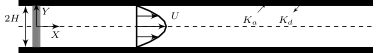
Figure 1: In an infinitely long channel, a slender, transversely uniform strip of solute (gray area) is released in the fluid and transported by Poiseuille flow with adsorption and desorption on the walls.

We model single component solute transport in a two-dimensional straight channel with surface adsorption and desorption, which is illustrated in figure 1. The width of the channel is $2H$ in the $Y$ direction and the length is assumed to be infinite in the $X$ direction. The velocity field is given by an ideal Poiseuille flow, $U(Y)=\frac{3}{2}U_{0}\left(1-Y^{2}/H^{2}\right)$, where $U_{0}$ is the mean flow velocity. Adsorption onto and desorption from the walls allow exchange of mass between the solid surface and the fluid.

The mass transport of solute in the fluid is given by the advection–diffusion equation,

$$\frac{\partial C}{\partial T}+U(Y)\frac{\partial C}{\partial X}=D\left(\frac{\partial^{2}C}{\partial X^{2}}+\frac{\partial^{2}C}{\partial Y^{2}}\right),$$ (1)

where $T$ is the dimensional time [$\text{\,}\mathrm{T}$], $C$ the dimensional solute concentration [$\text{\,}\mathrm{M}\mathrm{L}^{-3}$] and $D$ the diffusion coefficient [$\text{\,}\mathrm{L}^{2}\mathrm{T}^{-1}$].

Since the channel is assumed to be infinite, the concentration and any order of its derivative must vanish as $X\rightarrow\pm\infty$. Because of the symmetry along the centerline, $\partial C/\partial Y=0$, and only the upper half of the domain is considered.

The adsorbed concentration on the wall is assumed to form an infinitely-thin and static surface layer without longitudinal diffusion. The exchange of mass between the wall and the fluid is given as

$$-D\frac{\partial C}{\partial n}=\frac{\partial\varGamma}{\partial T},$$ (2)

where $n$ denotes the outward normal direction of the wall and $\varGamma$ is the dimensional surface concentration [$\text{\,}\mathrm{M}\mathrm{L}^{-2}$]. Adsorption and desorption are assumed to be described by the first-order reactions, so that the change of surface concentration is given by

$$\frac{\partial\varGamma}{\partial T}=K_{a}C-K_{d}\varGamma,$$ (3)

where $K_{a}$ and $K_{d}$ are the dimensional adsorption and desorption rate constants with dimensions of [$\text{\,}\mathrm{L}\mathrm{T}^{-1}$] and [$\text{\,}\mathrm{T}^{-1}$], respectively (Khan, 1962). When $K_{d}=0$, the linear kinetic model reduces to a first-order, irreversible adsorption reaction. When both $K_{a}$ and $K_{d}$ are large, the reaction approaches local chemical equilibrium. At equilibrium, the surface concentration is linearly proportional to solute concentration

$$\varGamma=KC,$$ (4)

where $K=K_{a}/K_{d}$ is the dimensional partition coefficient. Equation (4) is also referred to as a linear isotherm (Golay, 1958).

Initially, the solute has a uniform transverse distribution at $X=0$ with no mass adsorbed on the wall and is assumed to be a $\delta$-function in the $X$ direction so that C(X, Y, 0) = MIA   δ(X)  and  Γ(X, 0) = 0, where $M_{I}$ represents the total mass in the system [$\text{\,}\mathrm{M}$] and $A$ is the cross-sectional area of the channel [$\text{\,}\mathrm{L}^{2}$]. A characteristic concentration is chosen as $C_{0}=M_{I}/(HA)$ to simplify the formulation in dimensionless form. This initial condition, which has been used in previous work, assumes that the system is not in local chemical equilibrium. We note that the transient solute transport behavior is very sensitive to the initial condition and further analysis of the effect of the initial condition is provided in appendix A.

The following characteristic quantities are chosen to non-dimensionalize the problem,

$$\begin{array}[]{ccc}x=X/H,&y=Y/H,&u=U/U_{0},\\ c=C/C_{0},&\gamma=\varGamma/(C_{0}H),&t=T/(H^{2}/D).\end{array}$$ (5)

Note that we choose $C_{0}H$ as characteristic surface concentration and the diffusive time scale $H^{2}/D$ as the characteristic time scale. Consequently, the dimensionless formulation of the problem is written as

$$\frac{\partial c}{\partial t}+\mbox{{Pe}}\,u\frac{\partial c}{\partial x} =\frac{\partial^{2}c}{\partial x^{2}}+\frac{\partial^{2}c}{\partial y^{2}}$$ (6a)

$$-\frac{\partial c}{\partial y} =\frac{\partial\gamma}{\partial t}\quad\mbox{at\ }\quad y=1,$$ (6b)

$$\frac{\partial c}{\partial y} =0\quad\mbox{at\ }\quad y=0,$$ (6c)

$$c =\delta(x)\quad\mbox{at\ }\quad t=0,$$ (6d)

$${\color[rgb]{0,0,0}\gamma} {\color[rgb]{0,0,0}=0\quad\mbox{at\ }\quad t=0.}$$ (6e)

If the surface reaction is modelled by the linear kinetic model,

$$\frac{\partial\gamma}{\partial t}={k_{a}}c-{k_{d}}\gamma\,,$$ (7)

there will be three dimensionless groups in equation (6) and (7),

$$\mbox{{Pe}}=\frac{U_{0}H}{D},\quad{k_{a}}=\frac{K_{a}H}{D},\quad{k_{d}}=\frac{K_{d}H^{2}}{D}.$$ (8)

Physically, the Peclet number, Pe, represents the ratio of the transverse diffusive time scale to the longitudinal advective time scale and the Damköhler numbers, $k_{a}$ and $k_{d}$, represent the ratio of the transverse diffusive time scale to the adsorption and desorption time scales, respectively.

Otherwise, if the equilibrium sorption model is used

$$\gamma={k}c,$$ (9)

and the number of dimensionless groups reduces to two by replacing ${k_{a}}$ and ${k_{d}}$ with

$${k}=\frac{{k_{a}}}{{k_{d}}}.$$ (10)

In this work, ${k_{a}}$, ${k_{d}}$ and ${k}$ are all assumed to be constants. A value of $10$ is chosen for Pe to limit the longitudinal domain size required in numerical simulation. This choice will not affect the key results which are independent of Pe. In the following, we deal with the more general linear kinetic sorption model analytically and results will be given for both the kinetic and equilibrium model in §4.

3 Solution for the longitudinal moments

Following the classical, transverse-averaging idea introduced by Taylor (1953) to reduce the dimension of the problem, we consider the transverse-averaged concentration $\bar{c}=\int_{0}^{1}c\,dy$ and the distribution of $\bar{c}$ is described by its longitudinal moments $m_{n}=\int_{-\infty}^{\infty}x^{n}\bar{c}dx$, where $n$ is the order of the moment. The lower-order moments, e.g. zeroth-, first- and second-order moments are of most interest to us. Furthermore, we define the normalized longitudinal moments of zeroth-, first- and second-order M_0 = m0mI,  M_1 = m1m0,  M_2 = m2m0 - (m1m0 )^2, where ${m_{\mathrm{I}}}$ is the dimensionless initial mass, which is unity here. The fraction of solute in the fluid is given by $M_{0}$. The center of mass and the variance of the solute distribution in the fluid are given by $M_{1}$ and $M_{2}$, respectively. Thus, the dimensionless transport velocity and longitudinal dispersion coefficient are v = d M1d t  and  D_L = 12 d M2d t. In the following, analytical solutions are derived for lower order moments $m_{n}(n=0,1,2)$ in the form of series solutions.

3.1 Moment equation and solution in the Laplace space

Firstly, following the method of moments developed by Aris (1956), multiply equation (6a) by $x^{n}$ and integrate in the $x$ direction to obtain the equation for $c_{n}^{*}(y,t)$,

$$\frac{\partial c_{n}^{*}}{\partial t}+\mbox{{Pe}}\,u\int\limits_{-\infty}^{\infty}x^{n}\frac{\partial c}{\partial x}dx=\int\limits_{-\infty}^{\infty}x^{n}\frac{\partial^{2}c}{\partial x^{2}}dx+\frac{\partial^{2}c_{n}^{*}}{\partial y^{2}},$$ (11)

where $c_{n}^{*}=\int_{-\infty}^{\infty}x^{n}c\,dx$ is the $n^{\text{th}}$ longitudinal moment of concentration in the filament through $y$, which is not yet transversely averaged. The moments $m_{n}$ introduced above are the transverse averages of $c_{n}^{*}$. After integration by parts and noting that the concentration and all of its derivatives vanish at infinity, we have

$$\frac{\partial c_{n}^{*}}{\partial t}-n\mbox{{Pe}}\,u\,c_{n-1}^{*}=n(n-1)c_{n-2}^{*}+\frac{\partial^{2}c_{n}^{*}}{\partial y^{2}},$$ (12a)

where $$c_{-1}^{*}=c_{-2}^{*}=0$$. Similarly, the boundary conditions (6b) and (6c) give

$$-\frac{\partial c_{n}^{*}}{\partial y} =\frac{\partial\gamma_{n}^{*}}{\partial t}={k_{a}}c_{n}^{*}-{k_{d}}\gamma_{n}^{*}\quad\mbox{at\ }\quad y=1,$$ (12b)

$$\frac{\partial c_{n}^{*}}{\partial y} =0\quad\mbox{at\ }\quad y=0,$$ (12c)

where $\gamma_{n}^{*}$ is defined as the $n^{\text{th}}$ longitudinal moment of the surface concentration.

Laplace transform in time reduces (12) to a system of ordinary differential equations only involving the transformed variable

$${\hat{c\mkern 3.0mu}\mkern-3.0mu}{}_{n}^{*}(y,s)=\mathscr{L}\{c_{n}^{*}\}(s)=\int\limits_{0}^{\infty}c_{n}^{*}e^{-st}dt,$$ (13)

because the transformed longitudinal moments of surface concentration ${\hat{\gamma\mkern 3.0mu}\mkern-3.0mu}{}_{n}^{*}=\mathscr{L}\{\gamma_{n}^{*}\}$ in the boundary condition can be eliminated. In Laplace space, equations (12) are given by

$$\frac{\partial^{2}{\hat{c\mkern 3.0mu}\mkern-3.0mu}{}_{n}^{*}}{\partial y^{2}} =s{\hat{c\mkern 3.0mu}\mkern-3.0mu}{}_{n}^{*}-c_{n}^{*}(t=0)-n\mbox{{Pe}}\,u\,{\hat{c\mkern 3.0mu}\mkern-3.0mu}{}_{n-1}^{*}-n(n-1){\hat{c\mkern 3.0mu}\mkern-3.0mu}{}_{n-2}^{*},$$ (14a)

$$-\frac{\partial{\hat{c\mkern 3.0mu}\mkern-3.0mu}{}_{n}^{*}}{\partial y} =s{\hat{\gamma\mkern 3.0mu}\mkern-3.0mu}{}_{n}^{*}-\gamma_{n}^{*}(t=0)={k_{a}}{\hat{c\mkern 3.0mu}\mkern-3.0mu}{}_{n}^{*}-{k_{d}}{\hat{\gamma\mkern 3.0mu}\mkern-3.0mu}{}_{n}^{*}\quad\mbox{at\ }\quad y=1,$$ (14b)

$$-\frac{\partial{\hat{c\mkern 3.0mu}\mkern-3.0mu}{}_{n}^{*}}{\partial y} =0\quad\mbox{at\ }\quad y=0.$$ (14c)

Since no mass is adsorbed on the wall initially, $\gamma_{n}^{*}(t=0)=0$. A discussion of the more general initial conditions is given in appendix A. Note that the second equality in (14b) can be solved for ${\hat{\gamma\mkern 3.0mu}\mkern-3.0mu}{}_{n}^{*}$ as

$${\hat{\gamma\mkern 3.0mu}\mkern-3.0mu}{}_{n}^{*}=\frac{{k_{a}}}{{k_{d}}+s}{\hat{c\mkern 3.0mu}\mkern-3.0mu}{}_{n}^{*}.$$ (15)

so that (14b) turns into a Robin-type boundary condition

$$-\frac{\partial{\hat{c\mkern 3.0mu}\mkern-3.0mu}{}_{n}^{*}}{\partial y}=\frac{{k_{a}}s}{{k_{d}}+s}{\hat{c\mkern 3.0mu}\mkern-3.0mu}{}_{n}^{*}\quad\mbox{at\ }\quad y=1.$$ (16)

The $\delta$-function initial distribution of solute leads to the following initial conditions

$$c_{0}^{*}=1,\quad c_{1}^{*}=c_{2}^{*}=0\quad\mbox{at\ }\quad t=0.$$ (17)

Therefore, equation (14a), together with boundary conditions (14c) and (16), gives the following system of ordinary differential equations (ODEs) for ${\hat{c\mkern 3.0mu}\mkern-3.0mu}{}_{0}^{*}$, ${\hat{c\mkern 3.0mu}\mkern-3.0mu}{}_{1}^{*}$ and ${\hat{c\mkern 3.0mu}\mkern-3.0mu}{}_{2}^{*}$,

$$\frac{d^{2}{\hat{c\mkern 3.0mu}\mkern-3.0mu}{}_{0}^{*}}{dy^{2}} =s{\hat{c\mkern 3.0mu}\mkern-3.0mu}{}_{0}^{*}-1,$$ (18a)

$$\frac{d^{2}{\hat{c\mkern 3.0mu}\mkern-3.0mu}{}_{1}^{*}}{dy^{2}} =s{\hat{c\mkern 3.0mu}\mkern-3.0mu}{}_{1}^{*}-\mbox{{Pe}}\,u\,{\hat{c\mkern 3.0mu}\mkern-3.0mu}{}_{0}^{*},$$ (18b)

$$\frac{d^{2}{\hat{c\mkern 3.0mu}\mkern-3.0mu}{}_{2}^{*}}{dy^{2}} =s{\hat{c\mkern 3.0mu}\mkern-3.0mu}{}_{2}^{*}-2\mbox{{Pe}}\,u\,{\hat{c\mkern 3.0mu}\mkern-3.0mu}{}_{1}^{*}-2{\hat{c\mkern 3.0mu}\mkern-3.0mu}{}_{0}^{*},$$ (18c)

with boundary conditions

$$\frac{d{\hat{c\mkern 3.0mu}\mkern-3.0mu}{}_{n}^{*}}{dy} =-\frac{{k_{a}}s}{{k_{d}}+s}{\hat{c\mkern 3.0mu}\mkern-3.0mu}{}_{n}^{*}\quad\mbox{at\ }\quad y=1,$$ (19a)

$$\frac{d{\hat{c\mkern 3.0mu}\mkern-3.0mu}{}_{n}^{*}}{dy} =0\quad\mbox{at\ }\quad y=0,$$ (19b)

for $n=0,1,2$.

However, not the analytical solutions of ${\hat{c\mkern 3.0mu}\mkern-3.0mu}{}_{n}^{*}(y,s)$, but the transverse-averaged moments ${\hat{m\mkern 3.0mu}\mkern-3.0mu}{}_{n}(s)=\int_{0}^{1}{\hat{c_{n}^{*}\mkern 3.0mu}\mkern-3.0mu}{}dy$, are of interest here. For instance, ${\hat{m\mkern 3.0mu}\mkern-3.0mu}{}_{0}$ has the form

$${\hat{m\mkern 3.0mu}\mkern-3.0mu}{}_{0}=\frac{1}{s}-\frac{{k_{a}}\sinh\left(\sqrt{s}\right)}{\sqrt{s}\left({k_{a}}s\cosh\left(\sqrt{s}\right)+\sqrt{s}\sinh\left(\sqrt{s}\right)\left({k_{d}}+s\right)\right)}.$$ (20)

The analytical form of ${\hat{m\mkern 3.0mu}\mkern-3.0mu}{}_{1}$ and ${\hat{m\mkern 3.0mu}\mkern-3.0mu}{}_{2}$ are complex (given in supplementary materials), but both of them and ${\hat{m\mkern 3.0mu}\mkern-3.0mu}{}_{0}$ can be written in a general form as

$${\hat{m\mkern 3.0mu}\mkern-3.0mu}{}_{n}(s)=\frac{N_{n}(s)}{E(s)^{(n+1)}}\quad\text{for}\quad n=0,1,2,$$ (21)

where the denominator $E(s)$ is given by

$$E(s)={k_{a}}s\cosh\left({\sqrt{s}}\right)+\left({k_{d}}+s\right)\sqrt{s}\sinh\left({\sqrt{s}}\right),$$ (22)

which is a transcendental function of $s$ and includes all the singularities of the moments. The numerators $N_{n}(s)$ are complex functions of $s$ obtained by a computer algebra system (The MathWorks, Inc., 2012). The transcendental function $E(s)$ has two important properties:

1. There are only first-order singularities in $E(s)$, and thus ${\hat{m\mkern 3.0mu}\mkern-3.0mu}{}_{0}$, ${\hat{m\mkern 3.0mu}\mkern-3.0mu}{}_{1}$ and ${\hat{m\mkern 3.0mu}\mkern-3.0mu}{}_{2}$ only have first-, second- and third-order singularities, respectively. This helps to employ the residue theorem for the inverse Laplace transform.

2. All the singularities of $E(s)=0$ fall along the negative axis, and thus substituting $s=-p^{2}$, where $p$ is a real positive number, leads to a transcendental equation of $p$ in the real space ,

   $$\tan(p)(p^{2}-{k_{d}})-{k_{a}}p=0.$$ (23)

   Equation (23) has an infinite number of roots $p_{k},k=0,1,\dots,\infty$. These roots $p_{k}$ correspond to characteristic decay rates of the moments and the lowest order term with the smallest root, i.e. $p_{0}=0$, dominates the behavior at late times.

3.2 Inverse Laplace transform by the residue theorem

The inverse Laplace transform of the moments can be written as the Bromwich integral

$$m_{n}(t)=\frac{1}{2\upi\mathrm{i}}\int_{\mathcal{C}}{\hat{m\mkern 3.0mu}\mkern-3.0mu}{}_{n}(s)e^{st}ds,$$ (24)

where $\mathrm{i}=\sqrt{-1}$ and $\mathcal{C}$ is a contour chosen so that all the singularities of ${\hat{m\mkern 3.0mu}\mkern-3.0mu}{}_{n}(s)$ are to the left of it. Further, if we apply the residue theorem to the above integral, we have

$$m_{n}(t)=\sum\limits_{k=0}^{\infty}R_{k},$$ (25)

where $R_{k}$ are the residues of ${\hat{m\mkern 3.0mu}\mkern-3.0mu}{}_{n}e^{st}$ and can be calculated as

$$R_{k}=\frac{1}{(l-1)!}\lim_{s\to s_{k}}\frac{d^{l-1}}{ds^{l-1}}\left({\hat{m\mkern 3.0mu}\mkern-3.0mu}{}_{n}e^{st}(s-s_{k})^{l}\right).$$ (26)

where $l$ is the order of the $k^{\text{th}}$ singularity or pole $s_{k}$.

Since ${\hat{m\mkern 3.0mu}\mkern-3.0mu}{}_{0}$, ${\hat{m\mkern 3.0mu}\mkern-3.0mu}{}_{1}$ and ${\hat{m\mkern 3.0mu}\mkern-3.0mu}{}_{2}$ only have first-, second- and third-order singularities respectively, we have

$$m_{0}(t) =\sum\limits_{k=0}^{\infty}\lim_{s\to s_{k}}(s-s_{k}){\hat{m\mkern 3.0mu}\mkern-3.0mu}{}_{0}\exp(st)=\sum\limits_{k=0}^{\infty}a_{k}\exp(-p_{k}^{2}t),$$ (27a)

$$m_{1}(t) =\sum\limits_{k=0}^{\infty}\lim_{s\to s_{k}}\frac{d}{ds}\left[(s-s_{k})^{2}{\hat{m\mkern 3.0mu}\mkern-3.0mu}{}_{1}\exp(st)\right]=\sum\limits_{k=0}^{\infty}b_{k}^{(1)}\exp(-p_{k}^{2}t)+b_{k}^{(2)}t\exp(-p_{k}^{2}t),$$ (27b)

$$m_{2}(t) =\sum\limits_{k=0}^{\infty}\frac{1}{2}\lim_{s\to s_{k}}\frac{d^{2}}{ds^{2}}\left[(s-s_{k})^{3}{\hat{m\mkern 3.0mu}\mkern-3.0mu}{}_{2}\exp(st)\right]$$

$$=\sum\limits_{k=0}^{\infty}c_{k}^{(1)}\exp(-p_{k}^{2}t)+c_{k}^{(2)}t\exp(-p_{k}^{2}t)+c_{k}^{(3)}t^{2}\exp(-p_{k}^{2}t),$$ (27c)

where

$$a_{k} =\lim_{s\to s_{k}}(s-s_{k}){\hat{m\mkern 3.0mu}\mkern-3.0mu}{}_{0},$$ (28a)

$$b_{k}^{(1)} =\lim_{s\to s_{k}}\frac{d}{ds}\left[(s-s_{k})^{2}{\hat{m\mkern 3.0mu}\mkern-3.0mu}{}_{1}\right],$$ (28b)

$$b_{k}^{(2)} =\lim_{s\to s_{k}}(s-s_{k})^{2}{\hat{m\mkern 3.0mu}\mkern-3.0mu}{}_{1},$$ (28c)

$$c_{k}^{(1)} =\frac{1}{2}\lim_{s\to s_{k}}\frac{d^{2}}{ds^{2}}\left[(s-s_{k})^{3}{\hat{m\mkern 3.0mu}\mkern-3.0mu}{}_{2}\right],$$ (28d)

$$c_{k}^{(2)} =\lim_{s\to s_{k}}\frac{d}{ds}\left[(s-s_{k})^{3}{\hat{m\mkern 3.0mu}\mkern-3.0mu}{}_{2}\right],$$ (28e)

$$c_{k}^{(3)} =\frac{1}{2}\lim_{s\to s_{k}}(s-s_{k})^{3}{\hat{m\mkern 3.0mu}\mkern-3.0mu}{}_{2}.$$ (28f)

In order to remove the limit operator and give an explicit form of the coefficients in (28), the general form of moments in Laplace space (21) are substituted into (28). The fractional forms of ${\hat{m\mkern 3.0mu}\mkern-3.0mu}{}_{0}$, ${\hat{m\mkern 3.0mu}\mkern-3.0mu}{}_{1}$ and ${\hat{m\mkern 3.0mu}\mkern-3.0mu}{}_{2}$ allow us to apply the L’Hospital’s rule and obtain the explicit form of the coefficients,

$$a_{k} =\frac{N_{0}}{T_{1}},$$ (29a)

$$b_{k}^{(1)} =\frac{T_{1}N_{1}^{\prime}-2T_{2}N_{1}}{T_{1}^{3}},$$ (29b)

$$b_{k}^{(2)} =\frac{N_{1}}{T_{1}^{2}},$$ (29c)

$$c_{k}^{(1)} =\frac{(12T_{2}^{2}-6T_{1}T_{3})N_{2}-6T_{1}T_{2}N_{2}^{\prime}+T_{1}^{2}N_{2}^{\prime\prime}}{2T_{1}^{5}},$$ (29d)

$$c_{k}^{(2)} =\frac{T_{1}N_{2}^{\prime}-3T_{2}N_{2}}{T_{1}^{4}},$$ (29e)

$$c_{k}^{(3)} =\frac{N_{2}}{2T_{1}^{3}},$$ (29f)

where $N_{n}^{\prime}=dN_{n}/ds$, $N_{n}^{\prime\prime}=d^{2}N_{n}/ds^{2}$ at $s=s_{k}$ and $T_{n}=E^{(n)}/n!$ is the $n^{\text{th}}$ order Taylor expansion coefficient of $E(s)$ at $s=s_{k}$. These coefficients can also be expressed in terms of $p_{k}$ by substituting $s_{k}=-p_{k}^{2}$. The analytical expressions of $a_{k}$, $b_{k}^{(1)}$, $b_{k}^{(2)}$, $c_{k}^{(1)}$, $c_{k}^{(2)}$, $c_{k}^{(3)}$ are given in the supplementary materials.

To summarize, for a given ${k_{a}}$ and ${k_{d}}$, equation (23) is first solved for a series of $p_{k}$, which are substituted into (29) to obtain the coefficients $a_{k}$, $b_{k}$ and $c_{k}$. The normalized longitudinal moments $M_{0}$, $M_{1}$ and $M_{2}$, the transport velocity $v$ and the dispersion coefficient $D_{L}$ are then determined by definitions (3) and (3).

3.3 Reduction to previous results

In the long time limit, when the zeroth-order terms dominate, the transport velocity and dispersion coefficient are

$$v_{0} =\frac{b_{0}^{(2)}}{a_{0}}=\mbox{{Pe}}\frac{{k_{d}}}{{k_{a}}+{k_{d}}}=\mbox{{Pe}}\frac{1}{{k}+1},$$ (30a)

$$D_{0} =\frac{1}{2}\left(\frac{c_{0}^{(2)}}{a_{0}}-\frac{2b_{0}^{(1)}b_{0}^{(2)}}{{a_{0}}^{2}}\right)=\frac{1}{1+{k}}+{\mbox{{Pe}}}^{2}\frac{2}{105}\frac{1+9{k}+25.5{k}^{2}}{(1+{k})^{3}}+\frac{\mbox{{Pe}}^{2}}{{k_{d}}}\frac{{k}}{(1+{k})^{3}},$$ (30b)

which are consistent with the results obtained in chromatography (Khan, 1962). For $k>0$, the transport velocity of the solute is slower than the mean flow velocity at late times.

At early but finite time, the first-order terms dominate and lead to an asymptotic velocity $v_{1}$ and dispersion coefficient $D_{1}$ given as v_1 = b1(2)a1  and  D_1 = 12 ( c1(2)a1 - 2b1(1)b1(2)a12 ). In the limiting case of ${k_{d}}=0$ analysed by Lungu & Moffatt (1982), the zeroth-order coefficients of the moments vanish, i.e. $a_{0}=b_{0}^{(2)}=b_{0}^{(1)}=c_{0}^{(3)}=c_{0}^{(2)}=c_{0}^{(1)}=0$. Therefore, the first-order terms dominate and lead to the following asymptotic transport velocity and dispersion coefficient,

$$v_{\text{LM}} =\frac{\mbox{{Pe}}\left(4\,{{{k_{a}}}}^{2}\,{p_{1}}^{2}+3\,{{{k_{a}}}}^{2}+3\,{{k_{a}}}+4\,p_{1}^{4}-3\,p_{1}^{2}\right)}{4\,p_{1}^{2}\,\left({{{k_{a}}}}^{2}+{{k_{a}}}+p_{1}^{2}\right)},$$ (31a)

$$D_{\text{LM}} =1+\Bigl{(}\mbox{{Pe}}^{2}\bigl{(}-8\,{k_{a}}^{6}\,p_{1}^{4}+150\,{k_{a}}^{6}\,p_{1}^{2}-315\,{k_{a}}^{6}-56\,{k_{a}}^{5}\,p_{1}^{4}+750\,{k_{a}}^{5}\,p_{1}^{2}$$

$$-945\,{k_{a}}^{5}-24\,{k_{a}}^{4}\,p_{1}^{6}+282\,{k_{a}}^{4}\,p_{1}^{4}+555\,{k_{a}}^{4}\,p_{1}^{2}-945\,{k_{a}}^{4}-192\,{k_{a}}^{3}\,p_{1}^{6}$$

$$+1560\,{k_{a}}^{3}\,p_{1}^{4}-540\,{k_{a}}^{3}\,p_{1}^{2}-315\,{k_{a}}^{3}-24\,{k_{a}}^{2}\,p_{1}^{8}-78\,{k_{a}}^{2}\,p_{1}^{6}+1455\,{k_{a}}^{2}\,p_{1}^{4}$$

$$-495\,{k_{a}}^{2}\,p_{1}^{2}-136\,{k_{a}}\,p_{1}^{8}+810\,{k_{a}}\,p_{1}^{6}+225\,{k_{a}}p_{1}^{4}-8\,p_{1}^{10}-210\,p_{1}^{8}+585\,p_{1}^{6}\bigr{)}\Bigr{)}$$

$$\Big{/}\Bigl{(}160\,p_{1}^{6}\bigl{(}{k_{a}}^{2}+{k_{a}}+p_{1}^{2}\bigr{)}^{3}\Bigr{)},$$ (31b)

where $p_{1}$ is determined by solving (23). Equations (31) are consistent with (3.4) and (3.11) given in Lungu & Moffatt (1982), except for a difference in notation. For ${k_{a}}>0$, the asymptotic transport velocity of the solute is faster than the mean flow velocity. Note that the early and late transport velocity $v_{1}$, $v_{0}$ have linear dependence on Pe and the early and late dispersion coefficient $D_{1}$, $D_{0}$ (excluding contribution from pure diffusion) have quadratic dependence on Pe so that the normalized ones defined in (4.2) below are generally independent of Pe.

3.4 Equilibrium sorption model

If the kinetics of the reactions are fast enough that local chemical equilibrium is valid, the linear kinetic sorption model reduces to the linear isotherm (i.e., equilibrium sorption model) $\gamma={k}c$, with ${k}={k_{a}}/{k_{d}}$. For the equilibrium sorption model, equation (23) becomes

$$\tan(p)=-{k}\,p,$$ (32)

which can be solved for a series of $p_{k}$. Taking the limit ${k_{a}}\rightarrow\infty,{k_{d}}\rightarrow\infty$ of (29) while keeping ${k_{a}}/{k_{d}}={k}$, the coefficients become only functions of the partition coefficient ${k}$, as expected.

3.5 First-order approximation of the series solution

For the general case when ${k_{d}}$ is not zero, the fast transport described by (31) may survive at early times before desorption has come into play. In this case, the general series solution of the moments (27) allows us to study the transition from fast transport at early times described by first-order terms to slow transport at late times described by zeroth-order terms.

The zeroth- and first-order terms corresponds to the residues $R_{0}$ and $R_{1}$ in (25). Figure 2(a) and 2(b) show the comparison of the zeroth-order approximation $R_{0}$ and first-order approximation $R_{0}+R_{1}$ with the numerical inversion of Laplace transform using Talbot’s method (Abate & Whitt, 2006; McClure, 2013). As expected, the first-order approximation $R_{0}+R_{1}$ captures the solution at both the early and the late times, while the zeroth-order approximation $R_{0}$ only describes the late time behavior. Additional tests show that the first-order approximation is sufficient to describe the solution for a large range of ${k_{a}}$ and ${k_{d}}$ after a short initial time. Therefore, we truncate the series solution (27) by retaining only the zeroth- and first-order terms,

$$m_{0} =a_{0}+a_{1}\exp(-p_{1}^{2}t),$$ (33a)

$$m_{1} =\bigl{(}{b_{0}^{(1)}}+{b_{0}^{(2)}}t\bigr{)}\,+\,\bigr{(}{b_{1}^{(1)}}+{b_{1}^{(2)}}t\bigr{)}\exp(-p_{1}^{2}t),$$ (33b)

$$m_{2} =\bigl{(}{c_{0}^{(1)}}+{c_{0}^{(2)}}t+{c_{0}^{(3)}}t^{2}\bigr{)}\,+\,\bigl{(}{c_{1}^{(1)}}+{c_{1}^{(2)}}t+{c_{1}^{(3)}}t^{2}\bigr{)}\exp(-p_{1}^{2}t),$$ (33c)

where the higher-order terms describing the very early time behavior are ignored.

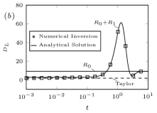
Figure 2: Comparison of the zeroth-order approximation ($R_{0}$) and the first-order approximation ($R_{0}+R_{1}$) with the numerical inversion of the Laplace transform (squares) using Talbot’s method. $R_{0}$ and $R_{1}$ are the zeroth and first residues of the moments defined in equation (25) and (26). Results are shown for $\mbox{{Pe}}=10,{k_{a}}=10,{k_{d}}=1$. Panel (a) shows the transport velocity $v$, where the mean flow velocity $u_{0}=U_{0}H/D=\mbox{{Pe}}$. Panel (b) shows the dispersion coefficient $D_{L}$, where the dashed line labelled as Taylor denotes the Taylor dispersion $2/105\mbox{{Pe}}^{2}$.

4 Regimes of transport

In this section, we discuss the transition from the early fast transport to the late slow transport. Numerical simulations of the full two-dimensional problem illustrate the physical mechanism that leads to this transition. The truncated analytical solution provides the estimates of the associated time scales. First, we will use the simpler equilibrium sorption model to discuss the regime transition, followed by the more general kinetic case.

4.1 Two-dimensional simulations

Figure 3 shows two-dimensional simulations of the solute concentration at different times for $\mbox{{Pe}}=10$, ${k_{a}}=50$ and ${k_{d}}=1$. The full problem is numerically solved by the Lattice Boltzmann Method (LBM) (Chen & Doolen, 1998; Wang & Kang, 2010; Zhang & Wang, 2015). The $\delta$-function initial condition is approximated by a piecewise constant function that is non-zero in a small interval around the origin. This approximation of the initial condition only affects the results in a short diffusive transient and the results agree well with the analytical solution (figure 3f-3h).

Initially, the strong adsorption removes the solute from the slow-moving fluid near the wall. The remaining solute in the center of the channel forms a fast-moving pulse (figure 3b and 3c), particularly evident in the transversely-averaged concentration shown in figure 3(e). This corresponds to the increased solute transport velocity in the irreversible sorption case (Lungu & Moffatt, 1982). This regime persists as long as adsorption dominates.

However, the fast-moving pulse decays rapidly and eventually desorption releases solute in its wake (figure 3d). As the amount of desorbed solute in the slow-moving fluid near the wall increases, the solute transport velocity declines. This process continues until desorption at the back balances adsorption at the front. The transport velocity and dispersion coefficient will approach the slow transport described by the one-dimensional model of the transversely-averaged concentration in the reversible sorption case (Khan, 1962).

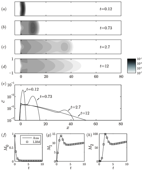
Figure 3: Two dimensional simulation of solute transport with sorption in Poiseuille flow with $\mbox{{Pe}}=10$, ${k_{a}}=50$ and ${k_{d}}=1$. Panel (a–d) show concentration distribution and panel (e) shows transversely-averaged concentration profile at $t=0.12,\,0.73,\,2.7,\,12$. Panel (f–h) show the evolution of the zeroth-, first- and second-order moments and compare the numerical simulation (LBM) with the first-order approximation of the analytical solution (Ana).

4.2 Equilibrium sorption model

Following the solution procedure in section 3.4, this section presents results and analysis for equilibrium sorption model, $\gamma={k}c$. To demonstrate the different transport behaviors, we define a normalized transport velocity $\mathcal{V}$ and a normalized dispersion coefficient $\mathcal{D}$ as V= vPe  and  D= DL- 1Dt, where $D_{t}=2/105\mbox{{Pe}}^{2}$ is the Taylor dispersion coefficient for a tracer in Poiseuille flow and the unit contribution of diffusion has been subtracted in the numerator of (4.2b). In this way, $\mathcal{V}>1$ ($\mathcal{D}>1$) means increased velocity (dispersion) relative to a nonreactive tracer while $\mathcal{V}<1$ ($\mathcal{D}<1$) means decreased velocity (dispersion).

Figure 4 shows the evolution of the position of the center of mass $M_{1}$ and the normalized transport velocity $\mathcal{V}$ for different partition coefficients. For ${k}>10$, a linear region emerges at early times in figure 4(a), corresponding to an initial plateau in figure 4(b). This corresponds to the well-developed early regime characterized by fast transport, approaching an asymptotic velocity $1+3/\upi^{2}\approx 1.3$. This is consistent with the results in an adsorption-only case with ${k_{a}}\rightarrow\infty$ (Lungu & Moffatt, 1982). After a transition period, a second linear region at late times appears, corresponding to the decreased transport velocity $1/(1+{k})$.

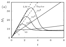
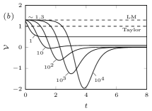
Figure 4: Evolution of (a) center of mass $M_{1}$ and (b) normalized transport velocity $\mathcal{V}$ for different partition coefficients ${k}$. Dashed lines with labels LM and Taylor stand for the asymptotic regime of an adsorption-only case (Lungu & Moffatt, 1982) and the asymptotic regime of a nonreactive tracer, respectively.

Figure 5 shows similar behaviors of the variance of solute mass in the fluid $M_{2}$ and the normalized dispersion coefficient $\mathcal{D}$. In the early regime, the dispersion coefficient is reduced relative to a tracer with $\mathcal{D}\sim 0.14$, which also agrees with the adsorption-only case with ${k_{a}}\rightarrow\infty$. In the late regime, the dispersion coefficient is given by the first two terms of (30b), first obtained by Golay (1958).

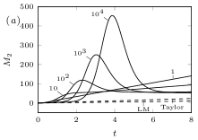
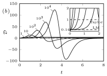
Figure 5: Evolution of (a) variance of solute mass distribution $M_{2}$ and (b) the normalized dispersion coefficient $\mathcal{D}$ for different partition coefficients ${k}$. Dashed lines with labels LM and Taylor stand for the asymptotic regime of an adsorption-only case (Lungu & Moffatt, 1982) and the asymptotic regime of a nonreactive tracer, respectively.

Between the early and late time, there is a drastic transition of the transport behavior. Especially when ${k}$ is large, both $M_{1}$ and $M_{2}$ decrease after reaching maxima during the transition and this leads to negative velocity and dispersion coefficient. Physically, it means that desorption near the origin dominates over the fast-moving pulse in figure 3 so that the center of mass shifts backwards and the variance reduces because the transversely-averaged concentration distribution changes from a bimodal type (one peak near the origin and the other at the pulse front) to a unimodal type (single peak near the origin).

To compare the early and late behaviors as a function of ${k}$, we define the normalized early and late velocities as V_e = v1Pe  and  V_l = v0Pe, and similarly we define normalized early and late dispersion coefficients as D_e = D1-1Dt  and  D_l = D0- 1/(1+k)Dt, where $v_{0}$, $D_{0}$ and $v_{1}$, $D_{1}$ are obtained from the zeroth- and first-order terms of the solution, the equilibrium limits of (30) and (3.3). Note that at early times the effective diffusion is not affected by sorption while it is reduced by a factor of $1/(1+k)$ at late times.

As shown in figure 6, for large ${k}$ the difference of normalized transport velocity between $\mathcal{V}_{e}$ and $\mathcal{V}_{l}$ is the largest and the normalized early-time dispersion coefficient $\mathcal{D}_{e}$ asymptotes to $0.14$. The normalized late-time dispersion coefficient $\mathcal{D}_{l}$ first increases with ${k}$, then reduces towards $0$. For small ${k}$, the early velocity $\mathcal{V}_{e}$ and dispersion coefficient $\mathcal{D}_{e}$ don’t reach the asymptotic values $1.3$ and $0.14$. In this case, the early regime is not well-developed and the first-order terms of the solution are not dominant. Therefore, $\mathcal{V}_{e}$ and $\mathcal{D}_{e}$ don’t represent the transport behavior in this case.

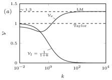
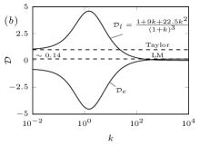
Figure 6: (a) Normalized early velocity $\mathcal{V}_{e}=v_{1}/\mbox{{Pe}}$, late velocity $\mathcal{V}_{l}=v_{0}/\mbox{{Pe}}$ and (b) normalized early dispersion coefficient $\mathcal{D}_{e}=(D_{1}-1)/D_{t}$, late dispersion coefficient $\mathcal{D}_{l}=(D_{0}-1/(1+{k}))/D_{t}$ as a function of partition coefficient ${k}$.

For a tracer in Poiseuille flow, the preasymptotic transport before equilibrium has been studied extensively (e.g. Gill & Sankarasubramanian, 1970; Haber & Mauri, 1988; Mercer & Roberts, 1990; Latini & Bernoff, 2001; Dentz & Carrera, 2007; Bolster et al., 2011; Wang et al., 2012). Typically, diffusion dominates when $t\ll t_{d}=\mbox{{Pe}}^{-2/3}$ and after the characteristic equilibrium time scale, $t=1$, solute transport can be described by the transversely-averaged model with the mean flow velocity and the dispersion coefficient $D_{t}$. However, for a reactive case considered here, the time scale to reach equilibrium can be quite different from the tracer case because surface reactions introduce additional characteristic time scales.

In the first-order approximation (33), a series of time scales can be defined by comparing the zeroth-order and first-order terms. Take $m_{0}$ as an example, by comparing $a_{0}$ and $a_{1}\exp(-p_{1}^{2}t)$, we can define a time scale as

$${\color[rgb]{0,0,0}t_{1}=\frac{1}{p_{1}^{2}}\ln\frac{a_{1}}{a_{0}}=\frac{1}{p_{1}^{2}}\ln\frac{2{k}^{2}({k}+1)}{{k}^{2}p_{1}^{2}+{k}+1}.}$$ (33)

This time scale indicates the transition from the early regime when the transport is dominated by the first-order terms to the late regime dominated by the zeroth-order terms. Similarly, other time scales can be determined by comparing $b_{k}$ and $c_{k}$. We notice that the coefficients in the series solution have the following property

$$\frac{a_{1}}{a_{0}}<\frac{{b_{1}^{(2)}}}{{b_{0}^{(2)}}}\sim\frac{{c_{1}^{(2)}}}{{c_{0}^{(2)}}}<\frac{{c_{1}^{(3)}}}{{c_{0}^{(3)}}},$$ (34)

which means that $t_{1}$ will give the smallest time scale. At the same time, since the time scales for the velocity determined by ${b_{1}^{(2)}}/{b_{0}^{(2)}}$ and the dispersion coefficient determined by ${c_{1}^{(2)}}/{c_{0}^{(2)}}$ have the same scaling, we can choose

$${\color[rgb]{0,0,0}t_{2}=\frac{1}{p_{1}^{2}}\ln\frac{{b_{1}^{(2)}}}{{b_{0}^{(2)}}}=\frac{1}{p_{1}^{2}}\ln\frac{{k}^{2}({k}+1)^{2}(4{k}^{2}p_{1}^{4}+3{k}^{2}p_{1}^{2}-3{k}+4p_{1}^{2}-3)}{2p_{1}^{2}({k}^{2}p_{1}^{2}+{k}+1)^{2}}}$$ (35)

as a critical time scale, after which the zeroth-order terms dominate and the late time behavior emerges. Note that both of the time scales are not dependent on Pe. Consequently, the transient solute transport with sorption can be divided into the following three regimes,

(I)	$0<t<t_{1}$	: early regime with fast transport
(II)	$t_{1}<t<t_{2}$	: transition period
(III)	$t_{2}<t$	: late regime with slow transport

As shown in figure 4 and 5, the duration of the early regime, as well as the transition period, increases with increasing ${k}$. In the limit of large ${k}$, we have lim_k→∞ t_1 = 42 lnk and  lim_k→∞ t_2 = 82 lnk, where we have used $\lim_{{k}\rightarrow\infty}p_{1}=\upi/2$. Equations (6) predict a linear relationship between $t_{1}$, $t_{2}$ and $\ln{{k}}$ when ${k}$ is large and $t_{2}\sim 2\,t_{1}$. Figure 7 compares results from the numerical inverse Laplace transform with these analytically determined time scales as a function of ${k}$. When ${k}\gg 1$, $t$ scales with $\ln{k}$, as predicted by (6). For small ${k}$, the early regime is so short that it is generally not observed.

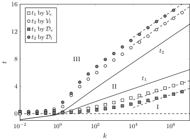
Figure 7: Variation of the early time scale $t_{1}$ and the late time scale $t_{2}$ as functions of different partition coefficient ${k}$. The solid lines show $t_{1}$ and $t_{2}$ from (33) and (35), respectively and the dashed lines indicate the scalings for large ${k}$ given by (6), which have been shifted to match the symbols determined by the numerical inverse Laplace transform. White symbols are determined by velocity and gray symbols are determined by dispersion coefficient. The transient solute transport with sorption is divided into three regimes: (I) early regime with fast transport; (II) transition period; (III) late regime with slow transport.

4.3 Kinetic sorption model

In the kinetic sorption model, there are two additional governing parameters, namely, the dimensionless adsorption rate constant ${k_{a}}$ and the dimensionless desorption rate constant ${k_{d}}$. Generally, a similar transition from early to late behavior can be observed and the equilibrium results are recovered when kinetics are fast, i.e. ${k_{a}}\gg 1$ and ${k_{d}}\gg 1$.

Similar to the way that the time scales are determined for the equilibrium model, we can obtain $t_{1}$ and $t_{2}$ for the kinetic model using (33) and (35),

$$t_{1} =\frac{1}{p_{1}^{2}}\ln\frac{2{k_{a}}^{2}({k_{a}}+{k_{d}})}{{k_{d}}\bigl{(}p_{1}^{4}+({k_{a}}^{2}+{k_{a}}-2{k_{d}})p_{1}^{2}+{k_{a}}{k_{d}}+{k_{d}}^{2}\bigr{)}},$$ (36a)

$$t_{2} =\frac{1}{p_{1}^{2}}\ln\frac{{k_{a}}^{2}({k_{a}}+{k_{d}})^{2}\bigl{(}4p_{1}^{6}+(4{k_{a}}^{2}-8{k_{d}}-3)p_{1}^{4}+(3{k_{a}}^{2}+3{k_{a}}+4{k_{d}}^{2}+6{k_{d}})p_{1}^{2}-3{k_{a}}{k_{d}}-3{k_{d}}^{2}\bigr{)}}{2{k_{d}}^{2}p_{1}^{2}\bigl{(}p_{1}^{4}+({k_{a}}^{2}+{k_{a}}-2{k_{d}})p_{1}^{2}+{k_{a}}{k_{d}}+{k_{d}}^{2}\bigr{)}^{2}},$$ (36b)

which are shown in figure 8.

The early regime is only observed when ${k_{a}}$ exceeds ${k_{d}}$. In all other cases, transition occurs from the very beginning followed by a dominated late regime. When both ${k_{a}}$ and ${k_{d}}$ are large, the time scales of the kinetic model recover those of the equilibrium model.

However, if the rates decrease, the kinetic time scales become longer. In this case, the root $p_{1}$ of (23) can be approximated by $p_{1}^{2}\approx{k_{a}}+{k_{d}}$ using Taylor expansion for $\tan(p)$. Then the ratios $a_{1}/a_{0}$ and ${b_{1}^{(2)}}/{b_{0}^{(2)}}$ used to obtain the time scales simplify to a1a0 = 2 kakd(ka+ 2)  and  b1(2)b0(2) = ka2(4ka+ 4kd+ 7)2 kd2(ka+ 2)2. This analysis shows that both time scales increase dramatically in the lower left region where ${k_{a}}$ and ${k_{d}}$ are small in figure 8. In this region, the duration of the early regime is long, but the deviations of velocity and dispersion coefficient from the tracer case are minor as the limiting values given by the adsorption-only case approach unity with small ${k_{a}}$. Physically, this region corresponds to a kinetically slow-sorbing (${k_{a}},{k_{d}}\ll 1$) solute with a large partition coefficient ${k}\gg 1$.

The analytical solution presented in §3.3 recovers the previous analysis in the limit of ${k_{d}}=0$ (Lungu & Moffatt, 1982). This limiting solution puts an upper bound on the transport velocity and a lower bound on the dispersion coefficient in the early regime. If the early regime is well-developed, the limiting solution given by Lungu & Moffatt (1982) provides a good approximation for finite ${k_{d}}$, see figure 8. The well-developed early regime is indicated by gray shadings in figure 8(a), where the early-time asymptotic transport velocity and dispersion coefficient given by (3.3) are within 10% of the limiting values given by Lungu & Moffatt (1982). Case A, B, C give examples of well-developed early regime, while the velocity doesn’t reach the asymptotic value in case D. Generally, if ${k}>10$ ($>1000$), the early-time velocity (dispersion coefficient) are well developed. Note that the first-order analytical solution for transport velocity ($R_{0}+R_{1}$) shown in figure 8(c) is computed by (3) and (33).

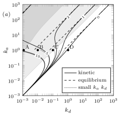
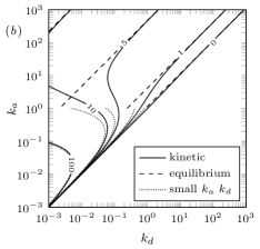
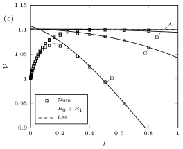
Figure 8: Contour lines of (a) the early time scale $t_{1}$ and (b) the late time scale $t_{2}$ for the kinetic sorption model. Dashed lines represent the time scales obtained from the equilibrium sorption model for large ${k_{a}}$ and ${k_{d}}$ and dotted lines represent approximations for small ${k_{a}}$ and ${k_{d}}$, given by (4.3). Shaded area in (a) represents the region where the early regime is well-developed, i.e., the velocity (light-shaded area) and dispersion coefficient (dark-shaded area) are close to the limiting values given by the adsorption-only case. Panel(c) shows the evolution of velocity at early time for the conditions labeled as A, B, C, D in panel(a). Symbols are the results from full numerical inverse Laplace transform, solid lines are first-order approximation of the analytical solution and dashed line is the asymptotic value for ${k_{d}}=0$ at ${k_{a}}=1$, given by Lungu & Moffatt (1982).

5 Conclusion

In this work, we reconcile two different analyses of solute transport with sorption in Poiseuille flow that reached apparently contradictory conclusions. We show that these two analyses capture different regimes of the transport. Generally, the solute experiences an early regime with fast transport velocity if adsorption dominates desorption. At late times, when desorption becomes important, the solute transport slows down. This leads to a regime transition that scales as $\ln{k}$ for the equilibrium sorption model, where ${k}$ is the dimensionless partition coefficient. Therefore, the early regime is more pronounced when ${k}$ is large. In the kinetic sorption model, the early regime is also observed if the kinetics are slow and the dimensionless adsorption rate constant ${k_{a}}$ exceeds the dimensionless desorption rate constant ${k_{d}}$. As long as ${k_{a}}\gg{k_{d}}$, the early regime is well-developed and the transport velocity and the dispersion coefficient in this early regime are well approximated by the analysis of Lungu & Moffatt (1982) in the limit of ${k_{d}}=0$.

The time scales presented in this work allow the determination of the dominant transport behavior for a given application. Experience shows that the late regime dominates the subsurface transport of sorbing contaminants in fractures. However, the early regime may be important in the biomedical applications where transport occurs over smaller distances. Our analysis may also allow a design of chromatography columns that can achieve opposite separation results.

Appendix A Effect of initial condition

The initial distribution of solute mass manifest itself either as a source term, $c_{n}^{*}(t=0)$, or a constant in the boundary condition, $\gamma_{n}^{*}(t=0)$, in the ODE system (18). These effects can be important in our problem in the sense that it may affect the form of the solutions of the moments. General discussion on this topic is out of the scope of this paper, and we show a special case as an example.

In the previous formulation, we assume initially there is no mass adsorbed on the wall, $\gamma_{n}^{*}(t=0)=0$. In this section, we change the initial condition by retaining the uniform release in the fluid, but assuming the mass distribution between the wall and the bulk has reached equilibrium, namely, $c(t=0)=\delta(x)/(1+{k})$, $\gamma(t=0)=\delta(x){k}/(1+{k})$. Following the same procedure in §3.1 and §3.2, we find that the moments in Laplace space ${\hat{m\mkern 3.0mu}\mkern-3.0mu}{}_{0},{\hat{m\mkern 3.0mu}\mkern-3.0mu}{}_{1},{\hat{m\mkern 3.0mu}\mkern-3.0mu}{}_{2}$ are no longer in the form of (21), but with a slight difference,

$${\hat{m\mkern 3.0mu}\mkern-3.0mu}{}_{0}(s) =\frac{Q_{0}(s)}{s},$$ (37a)

$${\hat{m\mkern 3.0mu}\mkern-3.0mu}{}_{1}(s) =\frac{Q_{1}(s)}{s\,E(s)},$$ (37b)

$${\hat{m\mkern 3.0mu}\mkern-3.0mu}{}_{2}(s) =\frac{Q_{2}(s)}{s\,E^{2}(s)},$$ (37c)

where $Q_{0}$, $Q_{1}$ and $Q_{2}$ are different from $N_{0}$, $N_{1}$ and $N_{2}$. In fact, $Q_{0}=1/(1+k)$. Essentially, the order of the all the singularities, other than the zeroth-order, reduce one in the solutions. Therefore, the series solutions obtained by residue theorem are written as

$$m_{0}(t) =a_{0},$$ (38a)

$$m_{1}(t) ={b_{0}^{(1)}}+{b_{0}^{(2)}}t+\sum\limits_{k=1}^{\infty}{\tilde{b\mkern 3.0mu}\mkern-3.0mu}{}_{k}^{(1)}\exp(-p_{k}^{2}t)$$ (38b)

$$m_{2}(t) ={c_{0}^{(1)}}+{c_{0}^{(2)}}t+{c_{0}^{(3)}}t^{2}+\sum\limits_{k=0}^{\infty}{\tilde{c\mkern 3.0mu}\mkern-3.0mu}{}_{k}^{(1)}\exp(-p_{k}^{2}t)+{\tilde{c\mkern 3.0mu}\mkern-3.0mu}{}_{k}^{(2)}t\exp(-p_{k}^{2}t).$$ (38c)

where ${\tilde{b\mkern 3.0mu}\mkern-3.0mu}{}_{k}^{(1)}$, ${\tilde{c\mkern 3.0mu}\mkern-3.0mu}{}_{k}^{(1)}$ and ${\tilde{c\mkern 3.0mu}\mkern-3.0mu}{}_{k}^{(2)}$ are different from $b_{k}^{(1)}$, $c_{k}^{(1)}$ and $c_{k}^{(2)}$. Note that the long-time velocity and dispersion coefficient determined by $a_{0}$, ${b_{0}^{(2)}}$, ${c_{0}^{(2)}}$ don’t change. However, since $b_{k}^{(2)}$ diminishes, the early regime will not be well-developed in this case. Physically, the solute that is initially adsorbed onto the wall begins to desorb much earlier, and hence reduces the duration of the early regime. In the limit of ${k_{d}}=0$, $k\rightarrow\infty$ and the initial solute mass in the fluid $c(t=0)$ vanishes so that the results by Lungu & Moffatt (1982) can not be properly recovered in this case.

References

- Abate & Whitt (2006) Abate, J. & Whitt, W. 2006 A unified framework for numerically inverting Laplace transforms. INFORMS J. Comput. 18 (4), 408–421.
- Aris (1956) Aris, R. 1956 On the dispersion of a solute in a fluid flowing through a tube. Proc. R. Soc. Lond. A 235 (1200), 67–77.
- Balakotaiah & Chang (1995) Balakotaiah, V. & Chang, H. C. 1995 Dispersion of chemical solutes in chromatographs and reactors. Phil. Trans. R. Soc. Lond. A 351 (1695), 39–75.
- Barton (1984) Barton, N. G. 1984 An asymptotic theory for dispersion of reactive contaminants in parallel flow. J. Aust. Math. Soc. B 25, 287–310.
- Biswas & Sen (2007) Biswas, R. R. & Sen, P. N. 2007 Taylor dispersion with absorbing boundaries: a stochastic approach. Phys. Rev. Lett. 98 (16), 164501.
- Bolster et al. (2011) Bolster, D., Valdés-Parada, F. J., LeBorgne, T., Dentz, M. & Carrera, J. 2011 Mixing in confined stratified aquifers. J. Contam. Hydrol. 120, 198–212.
- Chen & Doolen (1998) Chen, S. & Doolen, G.D. 1998 Lattice Boltzmann method for fluid flows. Annu. Rev. Fluid Mech. 30 (1), 329–364.
- De Gance & Johns (1978a) De Gance, A. E. & Johns, L. E. 1978a On the dispersion coefficients for Poiseuille flow in a circular cylinder. Appl. Sci. Res. 34 (2-3), 227–258.
- De Gance & Johns (1978b) De Gance, A. E. & Johns, L. E. 1978b The theory of dispersion of chemically active solutes in a rectilinear flow field. Appl. Sci. Res. 34 (2-3), 189–225.
- Dentz & Carrera (2007) Dentz, M. & Carrera, J. 2007 Mixing and spreading in stratified flow. Phys. Fluids 19 (1).
- Gill & Sankarasubramanian (1970) Gill, W. N. & Sankarasubramanian, R. 1970 Exact analysis of unsteady convective diffusion. Proc. R. Soc. Lond. A 316 (1526), 341–350.
- Golay (1958) Golay, M. J. E. 1958 Theory of chromatography in open and coated tubular columns with round and rectangular cross-sections. In Gas Chromatography (ed. D. H. Desty), pp. 36–53. Butterworths.
- Haber & Mauri (1988) Haber, S. & Mauri, R. 1988 Lagrangian approach to time-dependent laminar dispersion in rectangular conduits. part 1. two-dimensional flows. J. Fluid Mech. 190, 201–215.
- Hesse et al. (2010) Hesse, F., Harms, H., Attinger, S. & Thullner, M. 2010 Linear exchange model for the description of mass transfer limited bioavailability at the pore scale. Environ. Sci. Technol. 44 (6), 2064–71.
- Hlushkou et al. (2014) Hlushkou, D., Gritti, F., Guiochon, G., Seidel-Morgenstern, A. & Tallarek, U. 2014 Effect of adsorption on solute dispersion: a microscopic stochastic approach. Anal. Chem. 86 (9), 4463–70.
- Khan (1962) Khan, M. K. 1962 Non-equilibrium theory of capillary columns and the effect of interfacial resistance on column efficiency. In Gas Chromatography (ed. M. Van Swaay), pp. 3–17. Butterworths.
- Latini & Bernoff (2001) Latini, M & Bernoff, A. J. 2001 Transient anomalous diffusion in Poiseuille flow. J. Fluid Mech. 441, 399–411.
- Lungu & Moffatt (1982) Lungu, E. M. & Moffatt, H. K. 1982 The effect of wall conductance on heat diffusion in duct flow. J. Engng Math. 16 (2), 121–136.
- McClure (2013) McClure, T. 2013 Numerical inverse Laplace transform. Computer software. Mathworks File Exchange, Web. 1 Mar. 2016.
- Mercer & Roberts (1990) Mercer, G. N. & Roberts, A. J. 1990 A centre manifold description of contaminant dispersion in channels with varying flow properties. SIAM J. Appl. Math. 50 (6), 1547–1565.
- Mikelić et al. (2006) Mikelić, Andro, Devigne, Vincent & van Duijn, C. J. 2006 Rigorous upscaling of the reactive flow through a pore, under dominant Peclet and Damkohler numbers. SIAM J. Math. Anal. 38 (4), 1262–1287.
- Paine et al. (1983) Paine, M. A., Carbonell, R. G. & Whitaker, S. 1983 Dispersion in pulsed systems – I: Heterogenous reaction and reversible adsorption in capillary tubes. Chem. Eng. Sci. 38 (11), 1781–1793.
- Sankarasubramanian & Gill (1973) Sankarasubramanian, R. & Gill, W. N. 1973 Unsteady convective diffusion with interphase mass transfer. Proc. R. Soc. Lond. A 333 (1592), 115–132.
- Shapiro & Brenner (1986) Shapiro, M. & Brenner, H. 1986 Taylor dispersion of chemically reactive species: irreversible first-order reactions in bulk and on boundaries. Chem. Eng. Sci. 41 (6), 1417–1433.
- Shipley & Waters (2012) Shipley, R. J. & Waters, S. L. 2012 Fluid and mass transport modelling to drive the design of cell-packed hollow fibre bioreactors for tissue engineering applications. Math. Med. Biol. 29 (4), 329–59.
- Smith (1983) Smith, R. 1983 Effect of boundary absorption upon longitudinal dispersion in shear flows. J. Fluid Mech. 134, 161–177.
- Taylor (1953) Taylor, G. I. 1953 Dispersion of soluble matter in solvent flowing slowly through a tube. Proc. R. Soc. Lond. A 219 (1137), 186–203.
- The MathWorks, Inc. (2012) The MathWorks, Inc. 2012 MATLAB and Symbolic Toolbox Release 2012b. Natick, Massachusetts, United States.
- Wang et al. (2012) Wang, L., Cardenas, M. B., Deng, W. & Bennett, P. C. 2012 Theory for dynamic longitudinal dispersion in fractures and rivers with Poiseuille flow. Geophys. Res. Lett. 39 (5), l05401.
- Wang & Kang (2010) Wang, M. & Kang, Q. 2010 Modeling electrokinetic flows in microchannels using coupled lattice Boltzmann methods. J. Comput. Phy. 229 (3), 728–744.
- Wels et al. (1997) Wels, C., Smith, L. & Beckie, R. 1997 The influence of surface sorption on dispersion in parallel plate fractures. J. Contam. Hydrol. 28 (1-2), 95–114.
- Zhang & Wang (2015) Zhang, L. & Wang, M. 2015 Modeling of electrokinetic reactive transport in micropore using a coupled lattice Boltzmann method. J. Geophys. Res. 120 (5), 2877–2890.