Uplifting Anti-D6-brane

Abstract

A simple, KKLT-like construction of de Sitter vacua in type IIA string theory is presented in an STU model with guidance from string theory U-duality and with an uplifting anti-D6-brane. In four dimensions the model is reduced to $\mathcal{N}=1$ supergravity with three chiral multiplets, namely $S$, $T$ and $U$, as well as one nilpotent multiplet representing the anti-D6-brane. We briefly discuss also a generalization with seven moduli.

1 Introduction

Cosmological observations during the last two decades suggest that de Sitter and near de Sitter four-dimensional spacetimes are consistent with the data indicating a current and early universe acceleration. It is, however, notoriously difficult to derive de Sitter vacua from string theory compactified to four dimensions, as well as directly in a standard linearly realized four-dimensional supergravity.

It has been realized in Kachru:2003aw that, within type IIB string theory, de Sitter vacua can be obtained in a two-step procedure. First, using stringy perturbative and non-perturbative contributions to an effective superpotential, one can stabilize the volume of the extra dimensions in a supersymmetric anti-de Sitter vacuum. Secondly, with the help of an anti-D3-brane, one has to uplift this anti-de Sitter vacuum with a negative cosmological constant to a de Sitter vacuum with a positive cosmological constant. In four-dimensional $\mathcal{N}=1$ supergravity, this second step of the KKLT construction associated with the uplifting anti-D3-brane can be conveniently described by a non-linearly realized supersymmetry and a nilpotent multiplet Ferrara:2014kva ; Kallosh:2014wsa ; Bergshoeff:2015jxa ; Kallosh:2015nia ; Garcia-Etxebarria:2015lif ; Dasgupta:2016prs ; Vercnocke:2016fbt ; Kallosh:2016aep ; Bandos:2016xyu ; Aalsma:2017ulu ; GarciadelMoral:2017vnz ; Cribiori:2017laj ; Aalsma:2018pll ; Cribiori:2018dlc ; Cribiori:2019hod . A detailed derivation of the KKLT construction of de Sitter vacua from ten dimensions was presented recently in Hamada:2018qef ; Hamada:2019ack ; Carta:2019rhx ; Gautason:2019jwq ; Kachru:2019dvo .

Moduli stabilization in type IIA string theory was developed in Grimm:2004ua ; Villadoro:2005cu ; DeWolfe:2005uu ; Camara:2005dc , but consequently many no-go theorems for de Sitter minima were derived in Kallosh:2006fm ; Hertzberg:2007wc ; Haque:2008jz ; Flauger:2008ad ; Danielsson:2009ff ; Wrase:2010ew ; Shiu:2011zt ; Junghans:2016uvg ; Andriot:2016xvq ; Junghans:2016abx ; Andriot:2017jhf . A possibility of obtaining metastable de Sitter vacua in type IIA supergravity was proposed in Kallosh:2018nrk . It was explained there that, by adding pseudo-calibrated anti-Dp-branes wrapped on supersymmetric cycles, one can generalize the effective four-dimensional supergravity derived from string theory in a way that it includes a nilpotent multiplet. However, an explicit and simple KKLT-like two-step construction in type IIA string theory has not been presented so far.

In fact, in Kallosh:2018nrk an example with an anti-D6-brane is presented which had the following features. The starting point, before the introduction of the anti-D6-brane, is a de Sitter saddle point in linearly realized supergravity. When the action of the anti-D6-brane was added to the system, this saddle point became a de Sitter minimum in which all masses were positive. However, such a de Sitter minimum lied in fact below the de Sitter saddle point, as one can see in Fig. 1 of Kallosh:2018nrk . Therefore, this example presenting a stable local de Sitter vacuum in type IIA string theory was of a different nature with respect to the KKLT construction. In particular, the construction in Kallosh:2018nrk used only classical ingredients, making an exponentially small cosmological constant unnatural.

Nevertheless, one can take the results of Kallosh:2018nrk as a clear indication of the universality of the uplifting nature of pseudo-calibrated anti-Dp-branes wrapped on supersymmetric cycles. The purpose of this paper is therefore to explore constructions involving non-perturbative corrections, that give rise to anti-de Sitter vacua that can in turn be uplifted using anti-D6-branes. Related constructions that reproduce de Sitter vacua in the Large Volume Scenario Balasubramanian:2005zx in type IIA have already appeared in Palti:2008mg . Here we study constructions similar to the original KKLT model that use only a six-flux and non-perturbative corrections to the superpotential $W$ and an anti-D6-brane uplift.

2 The STU model

We will employ a simple STU model in order to exemplify how an uplift produced by an anti-D6-brane can be studied in a supergravity setup coming from type IIA string theory. The purpose of this section is therefore to outline such a model and to describe its ingredients.

2.1 The setup

In our notation which follows Dibitetto:2011gm ; Danielsson:2013rza , $S$ is the axio-dilaton, $T$ is a complex structure modulus and $U$ is the volume (Kähler) modulus. We propose to use ten-dimensional supergravity compactified on a calibrated manifold, like a Calabi-Yau manifold or a more general SU(3)-structure manifold, such that the standard, linearly realized four-dimensional $\mathcal{N}=1$ supergravity follows. This construction will be supplemented by pseudo-calibrated $\overline{D6}$-branes in order to facilitate a KKLT-like uplift.

To make our example concrete, we follow Danielsson:2013rza and consider a $T^{6}/(\mathbb{Z}_{2}\times\mathbb{Z}_{2})$ orbifold compactification of type IIA string theory with the ten-dimensional metric

$$ds^{2}_{10}=\tau^{-2}ds^{2}_{4}+\rho(\sigma^{-3}G_{ab}dy^{a}dy^{b}+\sigma^{3}G_{ij}dy^{i}dy^{j})\,.$$ (1)

Here the universal moduli $\rho$, $\tau$ and $\sigma$ are identified as

$$\rho ={\rm Im}(U)=(vol_{6})^{\frac{1}{3}},$$ (2)

$$\tau ={\rm Im}(S)^{\frac{1}{4}}{\rm Im}(T)^{\frac{3}{4}}=e^{-\phi}\sqrt{vol_{6}},$$

$$\sigma ={\rm Im}(S)^{-\frac{1}{6}}{\rm Im}(T)^{\frac{1}{6}},$$

while $G_{ab}$ and $G_{ij}$ correspond to the two independent three-cycles. To this construction we add $N_{\overline{D6}}^{||}$ and $N_{\overline{D6}}^{\bot}$ anti-D6-branes wrapping three-cycles. The first set of branes extends completely along only one cycle, while the second set corresponds to branes wrapping directions along both cycles, in all the possible combinations.

After compactifying to four dimensions, the total scalar potential is given by the sum of two pieces

$$V_{\rm tot}=V_{\mathcal{N}=1}+V_{\overline{D6}}\,,$$ (3)

where

$$V_{\mathcal{N}=1}=e^{K}\left(g^{i\bar{\jmath}}D_{i}WD_{\bar{\jmath}}\bar{W}-3W\bar{W}\right)\,,\qquad i=\{S,T,U\},$$ (4)

is the standard $\mathcal{N}=1$ supergravity scalar potential and

$$V_{\overline{D6}}={\mu_{1}^{4}\over{\rm Im}\,(T)^{3}}+{\mu_{2}^{4}\over{\rm Im}\,(T)^{2}{\rm Im}\,(S)}\,$$ (5)

is the contribution of the anti-D6-branes. The quantities $\mu_{1}^{4}=2e^{\mathcal{A}_{1}}N_{\overline{D6}}^{||}$ and $\mu_{2}^{4}=2e^{\mathcal{A}_{2}}N_{\overline{D6}}^{\bot}$ correspond to anti-D6-branes wrapped on two types of three cycles that are placed in potentially warped regions with warp factors $e^{\mathcal{A}_{1}}$ and $e^{\mathcal{A}_{2}}$, respectively.

The Kähler and superpotential for our model are

$$K =-\log\left(-{\rm i}(S-\bar{S})\right)-3\log\left(-{\rm i}(T-\bar{T})\right)-3\log\left(-{\rm i}(U-\bar{U})\right)\,,$$ (6)

$$W =f_{6}+W_{np}\,,$$

where $f_{6}$ is the flux parameter for a six-flux and the non-perturbative part $W_{np}$ of the superpotential is

$$W_{np}=\sum_{i}A_{i}e^{{\rm i}a_{i}\Phi_{i}},\qquad\qquad\Phi_{i}=\{S,T,U\}.$$ (7)

We furthermore assume that all of the parameters $f_{6}$, $A_{S}$, $A_{T}$, $A_{U}$, $a_{S}$, $a_{T}$ and $a_{U}$ are real and constant. Indeed, the parameters $A_{i}$ can, in principle, depend on the corresponding moduli $\Phi_{i}$ like $A_{i}(e^{\Phi_{i}})\approx A_{i}(0)+A^{\prime}_{i}(0)e^{-{\rm Im}\Phi_{i}}+\cdots$. However, for $e^{-{\rm Im}\Phi_{i}}\ll 1$ only the constant contribution will be significant. We will thus restrict our analysis to this case.

The non-perturbative part of the superpotential (7), involving $S$ and $T$, may arise from gaugino-condensation. Indeed, this effect can be parameterized by introducing terms of the form $e^{-a/g_{YM}^{2}}$ into the superpotential, where $a=\frac{2\pi}{N}$ and $g_{YM}$ is the coupling constant of the Yang-Mills theory living on $D6^{\parallel}$ or $D6^{\perp}$. It is possible to identify the coupling constants with the moduli $S$ and $T$ in the following way Danielsson:2013rza :

$$\frac{1}{\left(g_{YM}^{\parallel}\right)^{2}}\sim{\rm Im}(S),\qquad\qquad\frac{1}{\left(g_{YM}^{\perp}\right)^{2}}\sim{\rm Im}(T)\,.$$ (8)

Alternatively, Euclidean D2-branes wrapping internal 3-cycles will likewise give rise to such terms with $a_{S}=a_{T}=2\pi$. The origin of the non-perturbative term depending on the modulus $U$ will be motivated in the following subsection.

Note that, in principle, the superpotential can have the more generic form

$$W=f_{6}+f_{4}U+f_{2}U^{2}+f_{0}U^{3}+\left(h_{T}+r_{T}U\right)T+\left(h_{S}+r_{S}U\right)S+W_{np}\,,$$ (9)

with $f_{p}$ ($p=0,2,4,6$) arising from RR-fluxes, $h_{S/T}$ from integrating the NSNS-flux over the corresponding 3-cycles and $r_{S/T}$ from the curvature of the internal manifold. However, in complete analogy with the KKLT setup, which has the superpotential $W_{KKLT}=W_{0}+A_{\rho}e^{{\rm i}a_{\rho}\rho}$, we keep only $f_{6}$ and the non-perturbative exponents. Indeed, as we will discuss in appendix A for some examples, the inclusion of flux contributions, with the exception of $f_{6}$, seems to prohibit our uplift procedure from working.

There are many no-go theorems forbidding de Sitter vacua when only certain sets of classical ingredients are employed, see for example Kallosh:2006fm ; Hertzberg:2007wc ; Haque:2008jz ; Flauger:2008ad ; Danielsson:2009ff ; Wrase:2010ew ; Shiu:2011zt ; Junghans:2016uvg ; Andriot:2016xvq ; Junghans:2016abx ; Andriot:2017jhf . Recently it has been proposed that the inclusion of anti-D6-branes Kallosh:2018nrk ; Banlaki:2018ayh or KK monopoles Blaback:2018hdo can evade all no-go theorems and lead to classical, metastable dS vacua. In this work we evade the no-go theorems by including non-perturbative corrections that indeed turn out to be essential. Interestingly, our approach in this paper does not require a non-vanishing Romans mass parameter $f_{0}$ and therefore, contrary to the other constructions, it does allow for a direct lift to M-theory.

It is known that the KKLT construction provides a well working mechanism of stabilizing one complex modulus in an anti-de Sitter vacuum, assuming that the other moduli were already stabilized by perturbative terms in the superpotential. We will show that the same mechanism is also working well in each of the three complex moduli directions in our type IIA model. Indeed, we will follow a two-step procedure:

1. We stabilize all moduli using the six-flux and non-perturbative corrections. In this way we obtain a stable and supersymmetric anti-de Sitter vacuum, in which all of the fields have positive masses.

2. We then uplift the vacuum to de Sitter by adding anti-D6-branes, namely we introduce the corresponding terms with coefficients $\mu_{1}$ and $\mu_{2}$ in the scalar potential, as seen in equation (5).

We notice that, even if the first point is met, in general it is not guaranteed that the anti-de Sitter vacuum can consistently be uplifted to de Sitter. Indeed, examples in which the uplift fails are presented in the appendix A.2.

2.2 Satisfying stringy requirements

For a consistent embedding of our setup in type IIA string theory, we have to satisfy Gauss’ law in the compact space. This amounts to satisfying the Bianchi identities for the RR fields $F_{p}$. In our case for a compactification without 1- and 5-forms, the only non-trivial Bianchi identity is the tadpole condition for the D6-brane charges. It takes the form

$$\int dF_{2}-F_{0}H=-2N_{O6}+N_{D6}-N_{\overline{D6}}\,$$ (10)

and needs to be satisfied for each three-cycle independently. Since we are interested in very simple models with only non-vanishing $F_{6}$ flux, we have to satisfy the tadpole condition by adding D6-branes. These will cancel the negative contributions from the O6-planes and potential anti-D6-branes. In order to avoid instabilities due to the presence of D6-branes and anti-D6-branes, one has to find an appropriate geometry, which might be non-trivial (see for example Retolaza:2015sta ). Alternatively, together with non-perturbative effects from Euclidean D2-branes, one could try to also include more exotic O6-planes, like anti-O6-planes Kachru:1999ed or O$6^{+}$-planes. In particular, anti-O6-planes have negative tension but opposite RR-charge and this means that they would contribute to the tadpole condition in equation (10) with the same sign as D6-branes. Since they are non-dynamical, one would not have to worry about related instabilities. We leave a detailed study of this aspect to the future.

The RR- and NSNS-fluxes also have to be appropriately quantized. For us this means in particular that the parameters $f_{p}$ in the superpotential in equation (9) can assume only discrete values. We can easily set the $f_{6}$ parameter in equation (6) to any particular value by rescaling the superpotential. Indeed, this will change $f_{6}$ and the $A_{i}$ in (7) but neither the location nor the existence of the vacua.

Lastly, we would also like to ensure that higher order non-perturbative corrections, as well as $\alpha^{\prime}$ and string loop corrections, are suppressed. The general form of the non-perturbative corrections of the kind we are considering is a sum over all the instanton contributions

$$\sum_{n=1}^{\infty}A_{n}e^{{\rm i}na_{i}\Phi_{i}}$$ (11)

for all the fields $i=\{S,T,U\}$. However, in the non-perturbative superpotential in equation (7), for each of the moduli we are keeping only the very first term in the sum (11). To consistently neglect all the $n>1$ terms it is necessary to require that $a_{i}\text{Im}(\Phi_{i})>1$, $\forall i$. Additionally, in order to suppress $\alpha^{\prime}$ corrections and trust the supergravity approximation we need to require the volume of the internal manifold to be large, i.e. $vol(6)\gg 1$. Since in our setup $vol(6)=({\rm Im}(U))^{3}$, we will demand Im$(U)\gg 1$. Finally, string loop corrections are expected to be suppressed if Im$(S)\gg\tfrac{1}{16\pi^{2}}$. As we discuss in the next subsection, all of these requirements can be satisfied by using scaling symmetries of the STU model.

2.3 Scaling properties of the STU Model

From the previous discussion it seems that stringy requirements restrict the allowed positions of the critical points of the scalar potential. However, it is known since the racetrack inflation model BlancoPillado:2004ns that one can obtain models with rescaled values of the critical points for different choices of parameters, with respect to the original ones.

• In our STU model we notice that the kinetic terms are invariant under the rescaling

  $$S\rightarrow\lambda_{S}S\,,\qquad T\rightarrow\lambda_{T}T\,,\qquad U\rightarrow\lambda_{U}U.$$ (12)

  Indeed the Kähler potential changes only by an additive constant, namely $-\log(\lambda_{S}\lambda_{T}^{3}\lambda_{U}^{3})$, which can be compensated with a Kähler transformation. The resulting modification of the superpotential, then, can then be taken into account by rescaling of the parameters $a_{i}$

  $$a_{S}\rightarrow a_{S}/\lambda_{S}\,,\qquad a_{T}\rightarrow a_{T}/\lambda_{T}\,,\qquad a_{U}\rightarrow a_{U}/\lambda_{U},$$ (13)

  and by sending also $\{f_{6},A_{i}\}\to(\lambda_{S}\lambda_{T}^{3}\lambda_{U}^{3})^{\frac{1}{2}}\{f_{6},A_{i}\}$. Altogether, this implies that we can in fact rescale the positions of the anti-de Sitter minima from one set of fields $S$, $T$ and $U$, associated to a given choice of $a_{i}$, to another set with rescaled $a_{i}$ parameters. In the case in which the uplifting term is present, we also need to rescale

  $$\mu_{1}^{4}\rightarrow\mu_{1}^{4}\lambda_{T}^{3}\,,\qquad\mu_{2}^{4}\rightarrow\mu_{2}^{4}\lambda_{T}^{2}\lambda_{S}\,$$ (14)

  and send the nilpotent chiral multiplet $X\to(\lambda_{S}\lambda_{T}^{3}\lambda_{U}^{3})^{\frac{1}{2}}X$. This last ingredient will be introduced in section 6, in order to describe the anti-D6-brane contribution within an effective supergravity theory.

• We also notice that an overall rescaling of the scalar potential, namely $V\rightarrow c^{2}V$, can be achieved via

  $$f_{6}\rightarrow cf_{6}\,,\qquad A_{i}\rightarrow cA_{i}\,,\qquad\mu_{1}^{4}\rightarrow c^{2}\mu_{1}^{4}\,,\qquad\mu_{2}^{4}\rightarrow c^{2}\mu_{2}^{4}\,.$$ (15)

As a consequence of these transformations, we can change the parameters in the scalar potential as well as the critical points at which the moduli are stabilized. The presence of the (anti-)de Sitter minimum for the new parameters and critical points of the moduli is guaranteed by the rescaling properties of the theory.

3 The $U$-exponent issue

Two possible explanations of the non-perturbative terms in the $S$ and $T$ directions were given in Palti:2008mg , where it is argued that they can arise either from gaugino condensation on stacks of D6-branes or from Euclidean D2-branes. We also commented on this fact previously, near equation (8). On the other hand, the origin of the non-perturbative term in the volume modulus $U$ is less clear. We will discuss this issue in the present section.

We propose two arguments to justify the presence of exponential terms in $U$ in the non-perturbative superpotential.

1. The first reason is the concept/conjecture about string theory U-duality, which follows from M-theory. String theory tends to have S-duality and T-duality, which at the level of M-theory are expected to be combined into U-duality Hull:1994ys ; Schwarz:1996bh . This is known as a discrete U-duality symmetry, $E_{7}(\mathbb{Z})$, which contains the S-duality and T-duality groups as subgroup:

   $$E_{7}(\mathbb{Z})\supset SL(2,\mathbb{Z})\times O(6,6;\mathbb{Z})$$ (16)

   To this observation, one can add that the supersymmetric STU black holes, which have a symmetry known as string triality, have played a significant role in studies of the non-perturbative states of string theory, see for example Behrndt:1996hu . From this perspective it appears natural to expect that the non-perturbative exponential terms in $W$ are possible not only in the $S$ and $T$ directions, but also in the $U$ directions, since at the level of M-theory these moduli appear on equal footing, see for example Acharya:2007rc .

   The problem, however, is to identify a specific mechanism in type IIA string theory which is capable of producing the terms $e^{{\rm i}a_{U}U}$ in $W$, in addition to $e^{{\rm i}a_{S}S}$ and $e^{{\rm i}a_{T}T}$ as we define in equation (7) above. We may suggest that such term may originate from instantons, analogous to an Euclidean D3-brane wrapping a four-cycle in type IIB string theory, Witten:1996bn ; Kachru:2003aw . The problem here is that in the early studies of string theory instantons very often string theory moduli were viewed as constants, without the need to stabilize them as a function of the four-dimensional spacetime.

   In type IIA string theory we may think about instantons from an Euclidean NS5-brane wrapping a six-cycle. However, such instantons in the context of volume stabilization were already studied in Looyestijn:2008pg . It was conjectured there that these can only lead to corrections to the Kähler potential, since the volume itself cannot be expressed as a holomorphic function of the $\mathcal{N}=1$ chiral superfields. It would mean that NS5-brane instantons are not useful for our purpose. However, the argument/conjecture in Looyestijn:2008pg is not fully clear and might need to be revisited.

   If we look at earlier treatment of Fivebrane Instantons in Sec. 4 of Becker:1995kb , we may notice that the volume of the six-dimensional manifold is not present in their equations (4.1) and (4.2). The instanton action of the Fivebrane is given by

   $$e^{-S_{6}}=e^{-{1\over g_{s}^{2}}-{ia}},$$ (17)

   where $a$ is the axion field. There is no six-dimensional volume in this expression and it is not clear how to apply this to our situation. However, this form of the instanton action shows clearly that one of the U-duality symmetries, namely the axion shift symmetry of the theory which is part of the $SL(2,\mathbb{R})$ symmetry,

   $$a\rightarrow a+c,$$ (18)

   is broken unless $c=2\pi n$, where $n$ is an integer. This identification breaks the continuous $SL(2,\mathbb{R})$ symmetry down to its discrete $SL(2,\mathbb{Z})$ subgroup.

   Notice that the other parts of the $E_{7}(\mathbb{Z})$ U-duality symmetry mix our three moduli, $S$, $T$ and $U$, with some discrete parameters. To start with supergravity where we have a continuous U-duality and to end up with a discrete one, we need exponential terms involving axions, as we explained above, but we need them in all directions, including $U$.

   In the past, it was not always easy to find evidences of stringy U-duality, but many useful examples were found. Here, we will suggest to consider string wormholes Giddings:1989bq as a possible evidence towards U-duality and a possible source of the non-perturbative exponential for the modulus $U$. Indeed, consider the case in which the ten-dimensional theory is reduced to four dimensions by compactification on a six-dimensional Calabi-Yau (or other) manifold and assume that the ten-dimensional metric has a breathing mode, related to the volume modulus of the six-dimensional space. In this setup, the wormhole solution of Giddings:1989bq involves the radial axion and the breathing mode, which form a natural complex variable $Z=iU$. In particular, the real part of $Z(x)$ is related to a breathing mode field and the imaginary part is an axion field. The kinetic term for the complex field $Z$ was identified in Giddings:1989bq in equation (15). In this equation, we take a more recent standard normalization of the scalar curvature term in supergravity into account, with $1/2R$ as the Einstein term rather than $R$. Then the kinetic term of a modulus associated with the stringy wormhole becomes

   $$-3{\partial Z\partial\bar{Z}\over(Z+\bar{Z})^{2}}\,.$$ (19)

   This supports the identification of $Z$ with our volume modulus $U$. Thus, we find that the stringy wormholes presented in Giddings:1989bq suggest evidence for the existence of a non-perturbative exponential term in string theory associated with the modulus $U$, which in type IIA string theory describes the volume modulus or, using the earlier name, the breathing mode field of the ten-dimensional metric defined in equation (3) of Giddings:1989bq .

   This fact by itself does not tell us that such non-perturbative exponential terms in string theory, associated with the modulus $U$, have to appear in the superpotential $W$. The reasoning here which we suggest is the fact that in type IIA such exponential terms in the $S$ and in $T$ directions do appear. Thus, if U-duality is indeed a property of non-perturbative string theory, we can conclude that we do have a reasonable expectation that non-perturbative exponential terms for the modulus $U$ are possible in $W$. It would be very nice to understand these issues much better.

   In addition to this, open string worldsheet instantons in $\mathcal{N}=1$ orientifold compactifications of type IIA string theory are generically giving rise to the required exponential terms in $W$ that depend on the Kähler moduli Kachru:2000ih ; Blumenhagen:2009qh .

2. Our second reason to add an exponential in $U$ to the superpotential is the following. In type IIA string theory it was always difficult to find de Sitter vacua and even more difficult to find de Sitter minima. We will show below that with the new ingredients: non-perturbative exponents in $W$ in all directions and uplifting anti-D6-branes, building de Sitter vacua is not complicated anymore. In fact, our new cosmological model with all three exponents, respecting the U-duality symmetry of string theory, works extremely well for the purpose of getting anti-de Sitter minima, which in turn admit an uplifting via anti-D6-branes, producing de Sitter minima.

We can start now with the analysis of the model presented in section 2. Indeed, in the following two sections we will show how to construct de Sitter vacua in type IIA string theory.

4 Supersymmetric anti-de Sitter minimum

The first step in constructing a KKLT-like de Sitter vacuum is finding a stable anti-de Sitter vacuum of the $\mathcal{N}=1$ supergravity scalar potential (4). For stability in an anti-de Sitter spacetime it is sufficient to satisfy the well-known Breitenlohner-Freedman bound, which allows for negative mass values. However, in the present work we prefer to make a stronger request and ask that all the masses are positive. Indeed, we believe that such a situation is preferable in order to avoid instabilities at the step in which the anti-de Sitter vacuum will be uplifted to de Sitter.

To find a supersymmetric anti-de Sitter vacuum it is sufficient to solve the F-term equations

$$D_{i}W=0,\qquad i=\{S,T,U\},$$ (20)

using the Kähler potential and the superpotential given in (6) and (7). It is a known fact that these equations imply $\partial_{i}V=0$ but, importantly, not the other way around. For simplicity, at the supersymmetric anti-de Sitter minimum we set the axions to zero, namely those fields which receive a mass only through $W_{np}$:

$${\rm Re}\,(S)={\rm Re}\,(T)={\rm Re}\,(U)=0\,.$$ (21)

Such an assumption can be safely made as long as the masses in the vacuum are positive. Denoting the positions of the remaining fields at the minimum with

$${\rm Im}\,(S)=S_{0}\,,\qquad{\rm Im}\,(T)=T_{0}\,,\qquad{\rm Im}\,(U)=U_{0}\,,$$ (22)

we solve the equations (20) for the pre-exponential factors $A_{i}$ and find an expression for them in terms of the seven parameters of our choice:

$$A_{i}=A_{i}(f_{6},a_{S},a_{T},a_{U},S_{0},T_{0},U_{0})\,,\qquad i=\{S,T,U\}.$$ (23)

Notice that we are keeping $f_{6}$ as a free parameter. This choice will make the flux quantization straightforward to implement. Once the solution (23) is known, it is possible to check its stability by calculating the canonically normalized mass matrix

$${m_{i}}^{j}=\frac{1}{2}g^{jk}\nabla_{k}\partial_{i}V$$ (24)

at the minimum. Notice that, upon substituting (23), the mass matrix becomes a function of the aforementioned seven parameters: $m_{ij}=m_{ij}(f_{6},a_{S},a_{T},a_{U},S_{0},T_{0},U_{0})$.

As discussed in subsection 2.2, there are some restrictions that we need to impose on the general solution (23). A first requirement is related to the non-perturbative corrections. In order to consistently neglect higher order instanton contributions in the superpotential, we will choose the parameters $a_{i}$ such that $e^{-a_{i}\text{Im}(\Phi_{i})}$ is smaller than $\mathcal{O}(10^{-1})$ for each $i$ individually, i.e. along each field direction. Second, in order to trust the supergravity approximation of string theory, we have to require the volume of the internal manifold to be large. This will be implemented by choosing a sufficiently large value for the parameter $U_{0}$, $e.g.:$ $U_{0}\simeq\mathcal{O}(10)$. Finally, we will set the parameter $S_{0}$ to be $\mathcal{O}(1)$, such that string loop corrections are suppressed.

In the following we show that the class of stable and supersymmetric anti-de Sitter solutions (23) with the aforementioned restrictions is not empty. In particular, we will give two concrete examples of such solutions, corresponding to two different choices of the free parameters, and we will check that the masses in the vacuum are all positive. Since we find that the required properties hold, even for small variations of the parameters, we believe that solutions of the type (23) have a sufficiently large parameter space and are not isolated points.

4.1 Two specific anti-de Sitter solutions

As we will show in this subsection, by giving two explicit examples, it is not hard to find some set of parameters giving a solution of the type (23), with the desired properties. In both cases we set $S_{0}=T_{0}=1$ for simplicity and we choose $U_{0}=10$ in order to implement the large volume approximation. We then are left with four parameters, namely $f_{6}$ and the triplet $a_{i}$. Two possible choices for them are given in the following table.

	$f_{6}$	$a_{S}$	$a_{T}$	$a_{U}$
Set 1	$1$	$3$	$3$	$0.5$
Set 2	$2$	$3.1$	$3.3$	$0.32$

Table 1: The two sets of parameters that we investigated in detail. For both of them we find a stable anti-de Sitter vacuum with positive masses.

Notice that the parameter $a_{U}$ is roughly one order of magnitude smaller than $a_{S}$ and $a_{T}$, but the restriction $e^{-a_{U}U_{0}}<10^{-1}$ is still satisfied since $U_{0}$ is one order of magnitude bigger than $S_{0}$ and $T_{0}$. We can now check the stability of these two anti-de Sitter vacua by calculating the masses for the various fields. The results are reported in table 2.

	$m_{1}^{\,2}$	$m_{2}^{\,2}$	$m_{3}^{\,2}$	$m_{4}^{\,2}$	$m_{5}^{\,2}$	$m_{6}^{\,2}$
Set 1	$4.36\cdot 10^{-4}$	$3.79\cdot 10^{-4}$	$1.01\cdot 10^{-4}$	$7.37\cdot 10^{-5}$	$5.66\cdot 10^{-5}$	$3.64\cdot 10^{-5}$
Set 2	$1.19\cdot 10^{-3}$	$1.01\cdot 10^{-3}$	$2.43\cdot 10^{-4}$	$2.20\cdot 10^{-4}$	$1.64\cdot 10^{-4}$	$1.45\cdot 10^{-4}$

Table 2: The canonically normalized masses squared for both sets of parameters are all positive.

With the parameters given in table 1, we get the values for the $A_{i}$ and $e^{-a_{i}{\rm Im}\Phi_{i}}$, listed below in table 3. To check whether or not these make sense, we need to evaluate $A_{i}e^{-a_{i}{\rm Im}\Phi_{i}}$, which should be smaller than the tree level contribution of $f_{6}$, as discussed in section 2.2. This is the case for our values, which were indeed chosen to comply with these requirements.

	$A_{S}$	$A_{T}$	$A_{U}$	$e^{-a_{S}{\rm Im}S}$	$e^{-a_{T}{\rm Im}T}$	$e^{-a_{U}{\rm Im}U}$
Set 1	$-1.70$	$-5.11$	$-22.6$	$0.0498$	$0.0498$	$0.00674$
Set 2	$-3.43$	$-11.8$	$-11.0$	$0.0450$	$0.0369$	$0.0408$

Table 3: The resulting values for the parameters in front of the exponentials.

We did not encounter any particular difficulties in finding an appropriate choice for the parameters that yields an anti-de Sitter vacuum with the desired properties. For this reason, it seems plausible that a considerably large parameter space of working models exists. We notice that, when increasing the values of the parameters $a_{i}$, the masses approach zero. This is expected, since in the regime of large $a_{i}$ the non-perturbative corrections become small.

5 Uplifting anti-D6-branes and de Sitter minimum

In this section we show how the previously found anti-de Sitter vacua can be uplifted to de Sitter. For this purpose, we add a new ingredient, namely a certain number of anti-D6-branes, to the setup. We stress that, even if an anti-de Sitter vacuum with the desired properties is found, it is not guaranteed that it can be always uplifted to de Sitter. On the contrary, in many situations we looked at the uplift did not work, eventually giving one or more runaway directions. The very fact that we can uplift the two anti-de Sitter vacua presented in the previous section is a non-trivial result.

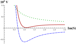
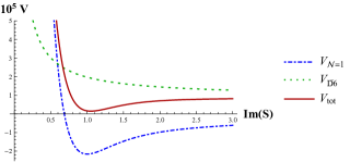
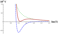
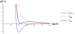
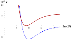
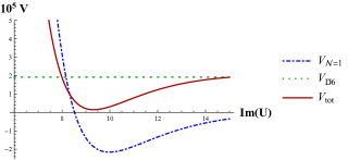
Figure 1: 2D plots of the total scalar potential $V_{tot}$, the anti-de Sitter potential $V_{\mathcal{N}=1}$ and the $\overline{D6}$ potential $V_{\overline{D6}}$. The left column of plots corresponds to Set 1 while the right is Set 2. Starting from the top we have the Im$(S)$ direction, followed by Im$(T)$ and Im$(U)$. In all plots we see clearly the anti-de Sitter and de Sitter vacua as well as the uplift term.

Therefore, let us add two sets of anti-D6-branes wrapping two 3-cycles in the internal manifold to the setup, as described in section 2 with the potential presented in equation (5). In section 6 we will explain how such an uplift term can be reproduced from a purely four-dimensional perspective by using a nilpotent chiral goldstino multiplet.

By appropriately tuning the parameters $\mu_{1}$ and $\mu_{2}$, it is possible to obtain de Sitter vacua in which the cosmological constant can be arbitrary small and we could even match it with the measured value at present. However, for convenience of the presentation, we choose the following values:

$$\text{Set 1}\qquad\mu_{1}^{4}=2.01\cdot 10^{-6},\qquad\mu_{2}^{4}=5.21\cdot 10^{-6},$$ (25)

$$\text{Set 2}\qquad\mu_{1}^{4}=\mu_{2}^{4}=1.34\cdot 10^{-5}.$$

After introducing the uplift, we need to check the stability of the resulting de Sitter vacua by calculating the masses of the various fields. The results are reported in table 4.

	$m_{1}^{\,2}$	$m_{2}^{\,2}$	$m_{3}^{\,2}$	$m_{4}^{\,2}$	$m_{5}^{\,2}$	$m_{6}^{\,2}$
Set 1	$3.43\cdot 10^{-4}$	$3.38\cdot 10^{-4}$	$6.46\cdot 10^{-5}$	$5.40\cdot 10^{-5}$	$4.15\cdot 10^{-5}$	$3.47\cdot 10^{-5}$
Set 2	$8.00\cdot 10^{-4}$	$7.40\cdot 10^{-4}$	$1.76\cdot 10^{-4}$	$1.63\cdot 10^{-4}$	$1.61\cdot 10^{-4}$	$1.50\cdot 10^{-4}$

Table 4: The canonically normalized masses squared after the uplift remain positive. This shows that the de Sitter vacua under investigation are metastable.

In figure 1, two-dimensional slices of the scalar potential are shown. The presence of the anti-de Sitter and de Sitter vacua described so far is clearly visible. We notice that the position of the minimum shifts after the uplift. This is expected since the addition of the anti-D6-branes modifies the form of the scalar potential. However, the actual shift is only up to a maximum of about $10\%$, which tells us that the masses are large enough to keep the minimum almost in place. In figure 2, three-dimensional plots of the scalar potential are shown for our Set 2 of parameters. Again, a metastable de Sitter minimum can clearly be seen.

               

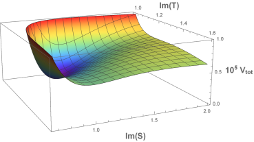
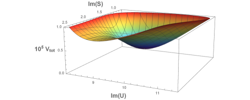
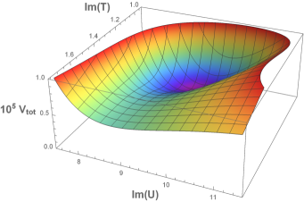
Figure 2: 3D plots of the de Sitter potential for the Set 2 of parameters. We have the following slices. Top: Im$(S)$ and Im$(T)$, Middle: Im$(S)$ and Im$(U)$, Bottom: Im$(U)$ and Im$(T)$. In all three different plots the de Sitter minimum is clearly visible and it is metastable.

We also checked that the total scalar potential is extremized at the position of the de Sitter vacuum, namely $\partial_{i}V_{tot}|_{\text{min}}=0$. We indeed find that this is the case within the limits of our numerical precision.

Finally, we noticed that one can also get metastable de Sitter vacua by including an anti-D6-brane uplift on either one of the two 3-cycles, i.e. by setting $\mu_{1}=0$ or $\mu_{2}=0$. It is also possible to use Euclidean D2-instantons instead of gaugino condensation on a stack of D6-branes by setting $a_{S}=2\pi$ and/or $a_{T}=2\pi$. Therefore, we see once more that this construction is rather robust and does not depend on any particular choice of parameters.

5.1 Simplifying or generalizing the setup

So far, we have described an STU model with three independent moduli. Such a model can be understood as a subcase of a more generic setup, with seven moduli, namely $S$, $T_{1}$, $T_{2}$, $T_{3}$, $U_{1}$, $U_{2}$ and $U_{3}$, in which we identified two sets of three moduli: $T_{1}=T_{2}=T_{3}\equiv T$ and $U_{1}=U_{2}=U_{3}\equiv U$. This corresponds to, for example, identifying three different tori of the compactification manifold. Along this logic, we can also set $T=S$ and arrive at the following simplified Kähler potential and superpotential:

$$K =-4\log\left(-{\rm i}(S-\bar{S})\right)-3\log\left(-{\rm i}(U-\bar{U})\right)\,,$$ (26)

$$W =f_{6}+A_{S}e^{{\rm i}a_{S}S}+A_{U}e^{{\rm i}a_{U}U}\,.$$

It is now interesting to ask whether or not this also leads to a viable model for a de Sitter uplift with anti-D6-branes. Indeed, it turns out that the construction of the model works out exactly in the same way as described in the previous sections. Even more interestingly, the same statement seems to be true for the generalization to the seven moduli case.

6 Four-dimensional action with $S$, $T$, $U$ and a nilpotent multiplet

As it was first studied in Kallosh:2018nrk and as we already mentioned before in the present work, it is possible to include the contribution from the anti-D6-branes to the scalar potential directly in the four-dimensional Kähler potential and superpotential. This is an example of the general fact that a nilpotent chiral goldstino superfield $X$, that satisfies $X^{2}=0$, can be used to include the contributions from anti-Dp-branes into the potentials.

A chiral multiplet satisfying $X^{2}=0$ has only one physical degree of freedom: the scalar is in fact given as a fermion bilinear. In superspace notation this means that the chiral superfield $X=\phi+\sqrt{2}\chi\theta+F\theta^{2}$, with the superspace coordinates $\theta$ and auxiliary field $F$, reduces to $X=\chi^{2}/(2F)+\sqrt{2}\chi\theta+F\theta^{2}$ upon enforcing the nilpotent constraint. An important feature of this method is that, after the inclusion of a nilpotent multiplet, supersymmetry will be realized non-linearly.

The general form of the Kähler potential and superpotential of four-dimensional $\mathcal{N}=1$ supergravity including a nilpotent chiral multiplet and coming from type IIA string theory is given in equation (35) of Kallosh:2018nrk (the nilpotent multiplet is called $S$ there). When specialized to our model, we find:

$$K= -\log\left(-{\rm i}(S-\bar{S})\right)-3\log\left(-{\rm i}(T-\bar{T})\right)$$ (27)

$$-\log\left(\left[-{\rm i}(U-\bar{U})\right]^{3}-\frac{X\bar{X}}{e^{\mathcal{A}_{1}}N_{\overline{D6}_{1}}\left(-{\rm i}(S-\bar{S})\right)+e^{\mathcal{A}_{2}}N_{\overline{D6}_{1}}\left(-{\rm i}(T-\bar{T})\right)}\right)\,,$$

$$W= f_{6}+A_{S}e^{{\rm i}a_{S}S}+A_{T}e^{{\rm i}a_{T}T}+A_{U}e^{{\rm i}a_{U}U}+\mu^{2}X\,.$$

Now we can calculate the scalar potential using the same formulas as before and implementing the nilpotency of $X$ at the end. Then, we compare the resulting expression with the one we obtained from the uplift in (5). They turn out to be exactly equal once we identify

$$\mu_{1}^{4}=\frac{1}{8}\mu^{4}e^{\mathcal{A}_{1}}N_{\overline{D6}_{1}},\qquad\qquad\mu_{2}^{4}=\frac{1}{8}\mu^{4}e^{\mathcal{A}_{2}}N_{\overline{D6}_{2}}.$$ (28)

This procedure has the obvious advantage that everything can be included in the four-dimensional supergravity description and shows once more the usefulness of non-linear supergravity.

7 Seven Moduli Model

The STU-model studied so far is actually a simplified version of a more general type IIA model with seven moduli, in which one identifies $T_{1}=T_{2}=T_{3}\equiv T$ and $U_{1}=U_{2}=U_{3}\equiv U$. In this section, we give some details of the analysis we performed on the seven-moduli model. In particular, following the same strategy as in the STU-model and by using anti-D6-branes, we have been able to find again stable de Sitter vacua even in the completely non-isotropy case.

The seven-moduli model, before the uplift, is described by the following Kähler potential and superpotential:

$$K =-\log\left(-{\rm i}(S-\bar{S})\right)-\sum_{i=1}^{3}\log\left(-{\rm i}(T_{i}-\bar{T}_{i})\right)-\sum_{i=1}^{3}\log\left(-{\rm i}(U_{i}-\bar{U}_{i})\right)\,,$$ (29)

$$W =f_{6}+A_{S}\,e^{{\rm i}a_{S}S}+\sum_{i=1}^{3}A_{T,i}\,e^{{\rm i}a_{T,i}T_{i}}+\sum_{i=1}^{3}A_{U,i}\,e^{{\rm i}a_{U,i}U_{i}}\,.$$

Once uplifting anti-D6-branes are introduced, they contribute to the scalar potential with the additional term

$$V_{\overline{D6}}= \frac{\mu_{1}^{\,4}}{Im(T_{1})Im(T_{2})Im(T_{3})}+\frac{\mu_{2}^{\,4}}{Im(S)Im(T_{2})Im(T_{3})}$$ (30)

$$+ \frac{\mu_{3}^{\,4}}{Im(S)Im(T_{1})Im(T_{3})}+\frac{\mu_{4}^{\,4}}{Im(S)Im(T_{1})Im(T_{2})}\,,$$

where $\mu_{1}$, $\mu_{2}$, $\mu_{3}$ and $\mu_{4}$ are parameters. Even in this case, the anti-D6-brane can be implemented into supergravity by means of a nilpotent chiral multiplet $X$. The resulting effective theory is a straightforward generalization of (27).

The analysis of the models (29) proceeds as usual. First, we find a stable and supersymmetric AdS vacuum, by solving the F-term equations $D_{i}W=0$. Again, we will give here only two different sets of parameters corresponding to two distinct solutions, but the choice we made is by no means exceptional. The parameters we used are reported in table 6.

	$S_{0}$	$T_{1,0}$	$T_{2,0}$	$T_{3,0}$	$U_{1,0}$	$U_{2,0}$	$U_{3,0}$
Set 1	$1$	$1$	$1$	$1$	$10$	$10$	$10$
Set 2	$1$	$1.4$	$1.5$	$1.6$	$11$	$12$	$13$
	$a_{S}$	$a_{T_{1}}$	$a_{T_{2}}$	$a_{T_{3}}$	$a_{U_{1}}$	$a_{U_{2}}$	$a_{U_{3}}$
Set 1	$3$	$3$	$3$	$3$	$0.5$	$0.5$	$0.5$
Set 2	$3.6$	$3.7$	$3.8$	$3.9$	$0.33$	$0.34$	$0.36$

Table 5: Two choices of the parameters for the seven-moduli model. In addition, we take $f_{6}=1$ for Set 1, while $f_{6}=3/\sqrt{2}$ for Set 2.

The values of the parameters $A_{i}$ and of the exponentials $e^{-a_{i}{\rm Im}\Phi_{i}}$ for these two solutions are reported in the following table.

	$A_{S}$	$A_{T_{1}}$	$A_{T_{2}}$	$A_{T_{3}}$	$A_{U_{1}}$	$A_{U_{2}}$	$A_{U_{3}}$
Set 1	$-1.70$	$-1.70$	$-1.70$	$-1.70$	$-7.55$	$-7.55$	$-7.55$
Set 2	$-6.09$	$-20.6$	$-31.4$	$-49.2$	$-6.22$	$-8.69$	$-13.8$
	$e^{-a_{S}{\rm Im}S}$	$e^{-a_{T_{1}}{\rm Im}T_{1}}$	$e^{-a_{T_{2}}{\rm Im}T_{2}}$	$e^{-a_{T_{3}}{\rm Im}T_{3}}$	$e^{-a_{U_{1}}{\rm Im}U_{1}}$	$e^{-a_{U_{2}}{\rm Im}U_{2}}$	$e^{-a_{U_{3}}{\rm Im}U_{3}}$
Set 1	$0.0499$	$0.0499$	$0.0499$	$0.0499$	$0.00674$	$0.00674$	$0.00674$
Set 2	$0.0273$	$0.00563$	$0.00335$	$0.00195$	$0.0265$	$0.0169$	$0.00928$

Table 6: The values of $A_{i}$ and of $e^{-a_{i}{\rm Im}\Phi_{i}}$ for the two anti-de Sitter solutions.

Then, we can uplift these vacua by introducing anti-D6-branes. We chose the following values for the uplifting parameters.

Set 1: $$\quad\mu_{1}^{\,4}=1.23\cdot 10^{-6},\quad\mu_{2}^{\,4}=1.23\cdot 10^{-6},\quad\mu_{3}^{\,4}=3.11\cdot 10^{-6},\quad\mu_{4}^{\,4}=2.14\cdot 10^{-6}.$$ (31)

Set 2: $$\quad\mu_{1}^{\,4}=5.52\cdot 10^{-6},\quad\mu_{2}^{\,4}=3.45\cdot 10^{-6},\quad\mu_{3}^{\,4}=3.68\cdot 10^{-6},\quad\mu_{4}^{\,4}=3.94\cdot 10^{-6}\,.$$

After the uplift, we find stable de Sitter vacua. The squared masses for the seven-moduli are reported in table 7, for both the de Sitter solutions.

	Set 1	Set 2
$m_{1}^{\,2}$	$3.33\cdot 10^{-4}\,$	$3.95\cdot 10^{-4}\,$
$m_{2}^{\,2}$	$3.32\cdot 10^{-4}$	$3.62\cdot 10^{-4}$
$m_{3}^{\,2}$	$1.55\cdot 10^{-4}$	$1.98\cdot 10^{-4}$
$m_{4}^{\,2}$	$1.55\cdot 10^{-4}$	$1.73\cdot 10^{-4}$
$m_{5}^{\,2}$	$1.44\cdot 10^{-4}$	$1.58\cdot 10^{-4}$
$m_{6}^{\,2}$	$1.44\cdot 10^{-4}$	$1.45\cdot 10^{-4}$
$m_{7}^{\,2}$	$6.31\cdot 10^{-5}$	$1.32\cdot 10^{-4}$
$m_{8}^{\,2}$	$4.99\cdot 10^{-5}$	$1.23\cdot 10^{-4}$
$m_{9}^{\,2}$	$4.13\cdot 10^{-5}$	$1.10\cdot 10^{-4}$
$m_{10}^{\,2}$	$4.13\cdot 10^{-5}$	$1.00\cdot 10^{-4}$
$m_{11}^{\,2}$	$4.11\cdot 10^{-5}$	$8.56\cdot 10^{-5}$
$m_{12}^{\,2}$	$3.52\cdot 10^{-5}$	$7.35\cdot 10^{-5}$
$m_{13}^{\,2}$	$3.08\cdot 10^{-5}$	$6.25\cdot 10^{-5}$
$m_{14}^{\,2}$	$2.85\cdot 10^{-5}$	$5.50\cdot 10^{-5}$

Table 7: The canonically normalized masses in the de Sitter vacuum for the seven-moduli case.

Once more, we stress that no particular fine tuning is necessary also for the uplift parameters. To conclude, we have shown that even in this more complicated seven-moduli scenario, the analysis proceeds exactly in the same way as in the STU-model that we discussed in detail in the previous sections.

8 Discussion

In the past, type IIA string theory was always viewed as a theory which is difficult to make compatible with cosmology Kallosh:2006fm ; Hertzberg:2007wc ; Haque:2008jz ; Flauger:2008ad ; Danielsson:2009ff ; Wrase:2010ew ; Shiu:2011zt ; Junghans:2016uvg ; Andriot:2016xvq ; Junghans:2016abx ; Andriot:2017jhf . A great effort in this direction was based on a complicated polynomial in $S$, $T$ and $U$ in the superpotential, as shown in equation (9), with four types of fluxes and also terms associated with the curvature of the compact manifold. Even with all these different contributions, it was not possible to easily produce de Sitter minima in type IIA string theory compactified to four dimensions.

The first, unexpected, result of this paper is that instead of a complicated polynomial in $S$, $T$ and $U$ in the superpotential, as shown in equation (9), one can use just a six-flux and non-perturbative exponential terms, given in equations (6) and (7) to stabilize all moduli in a supersymmetric anti-de Sitter minimum with all six mass eigenvalues positive. Thus, with the standard Kähler potential for the STU model in equation (6) and with the simple superpotential

$$W=f_{6}+A_{S}e^{{\rm i}a_{S}S}+A_{T}e^{{\rm i}a_{T}T}+A_{U}e^{{\rm i}a_{U}U}\,,$$ (32)

it is easy to find parameters which lead to anti-de Sitter minima.

The second result about the uplifting role of the anti-D6-brane was predicted in Kallosh:2018nrk , but not explicitly realized in the examples there. Here, we have found that the stable anti-de Sitter minima obtained in the STU model in equation (6) are upliftable to stable de Sitter minima, i.e. again we find all six mass matrix eigenvalues to be positive.

This situation has to be contrasted with our earlier efforts, which are reported in the appendix. In particular, we studied STU models where in addition to six-flux and non-perturbative corrections we engaged also other fluxes and curvature terms, like the ones shown in equation (9). In these setups, we have typically encountered tachyons in the anti-de Sitter extremum, which made these models unsuitable for uplifting. Another class of models with two moduli is presented in appendix A.2. It was obtained from the STU model after the identification $S=T$. It had the feature that the U-dependence in $W$ was polynomial, but in the S-direction we engaged two exponents, as in Kallosh:2004yh . As a result, we were able to find anti-de Sitter minima in these models, however, the anti-D6-brane uplift failed again: we were not able to find a stable de Sitter minimum for the complex $U$ and the complex $S$ directions.

In view of these failed examples it might sound puzzling as to why the simple model in (32) works well, whereas other models with a significant polynomial dependence on the moduli do not work. One explanation is that our new STU model can be qualified as (KKLT)³: we took a KKLT model, which is known to work in the case of one complex modulus, and we did the same with the other directions. Indeed, we just have a constant term and exponents in each direction in the superpotential. We have also learned that the no-scale structure of the Kähler potential is not really important here. In fact, our STU model leads to de Sitter minima for cases with different contribution to $K$: $-\log(-{\rm i}(S-\bar{S}))$, $-3\log(-{\rm i}(T-\bar{T}))$ and $-3\log(-{\rm i}(U-\bar{U}))$.

In section 7, we have also checked that the same principle works for the seven-moduli case, namely (KKLT)⁷, with

$$K=-\sum_{i=1}^{7}\log(-{\rm i}(\Phi_{i}-\bar{\Phi}_{i}))\,,\qquad W=f_{6}+\sum_{i=1}^{7}A_{i}e^{{\rm i}a_{i}\Phi_{i}}\,.$$ (33)

As we explained before, our STU model in equation (6) corresponds to the seven-moduli case where $T_{1}=T_{2}=T_{3}$ and $U_{1}=U_{2}=U_{3}$ are identified. Such a seven-moduli setup is particularly interesting with regard to the CMB B-mode targets Ferrara:2016fwe ; Kallosh:2017ced .

It would also be interesting to go beyond the simple STU model and study some other compactifications. In particular, the original GKP solution in type IIB Giddings:2001yu has been T-dualized to find type IIA no-scale Minkowski vacua, in which some of the moduli are stabilized by fluxes Kachru:2002sk ; Grana:2006kf ; Andriolo:2018yrz . These solutions have a build in tadpole cancellation condition and provide a natural starting point for the construction of dS vacua following the original KKLT approach, that we adapted and generalized here in the type IIA setting.

Appendix A How fluxes prohibit stable solutions

So far, in the literature (see for example Marchesano:2019hfb and references therein), tree-level contributions were usually employed in order to find de Sitter vacua, while in the present work we studied the opposite situation, which made the task much easier. For completeness, in this appendix we want to describe some models we investigated but that ultimately did not allow for a consistent uplift to de Sitter.

Our starting point was the same Kähler potential we used in the main part of this work, namely

$$K=-\log\left(-{\rm i}(S-\bar{S})\right)-3\log\left(-{\rm i}(T-\bar{T})\right)-3\log\left(-{\rm i}(U-\bar{U})\right)\,,$$ (34)

and the more general superpotential $W=W_{pert}+W_{np}$ including flux parameters not only for 6-form flux, but also 4-, 2- and 0-form flux, as well as non-perturbative corrections:

$$W_{pert} =f_{6}+f_{4}U+f_{2}U^{2}+f_{0}U^{3}+\left(h_{T}+r_{T}U\right)T+\left(h_{S}+r_{S}U\right)S\qquad\text{and}$$ (35)

$$W_{np} =A_{S}e^{{\rm i}a_{S}S}+A_{T}e^{{\rm i}a_{T}T}+A_{U}e^{{\rm i}a_{U}U}\,.$$

Again, we assume that all parameters, $f_{i}$, $i=0,2,4,6$, $A_{S},A_{T},A_{U}$ and $a_{S},a_{T},a_{U}$, are real.

Starting from these $K$ and $W$ we have a large amount of potential models. Indeed, our choices include identifying moduli, setting flux parameters and/or non-perturbative corrections to zero. It is important to note that one would expect that the non-perturbative contributions should not be significant when compared to the tree level in $W_{pert}$. This means we should set $A_{i}=0$, $i=\{S,T,U\}$, if the corresponding modulus appears at tree level.

A.1 STU models with fluxes

If one follows the logic concerning the coexistence of tree level and non-perturbative contributions lined out above, it seems that one generally arrives at an anti-de Sitter critical point that includes at least one tachyon. Indeed, while tuning the parameters does allow to modify the masses, we were not able to get rid of all tachyons: at least one mass remained negative. On one hand we were aware of the well-known no-go theorems in Hertzberg:2007wc ; Haque:2008jz ; Flauger:2008ad , that tell us that at least $f_{0}$ and $r_{S}$ or $r_{T}$ should be non-vanishing in order to get a de Sitter vacuum. On the other hand, since we evaded the no-go’s by including non-perturbative corrections, it is reasonable to consider models that do not obey these conditions.

Since we were not able to arrive at a stable anti-de Sitter vacuum with all masses positive, there is little hope that the uplift will lead to a stable de Sitter vacuum and thus we consider this class of models to be not viable.

A.2 A KL-type of model

In Kallosh:2004yh a modification of the non-perturbative terms was proposed where one includes two different exponentials for the same modulus. For a general modulus $Y$ this looks like

$$A_{Y}e^{{\rm i}a_{Y}Y}-B_{Y}e^{{\rm i}b_{Y}Y}\,$$ (36)

and it often improves the situation when the requirement that $e^{-a_{Y}\text{Im}(Y)}$ needs to be small is in the way of, for example, positive masses.

In fact in a model where we identified $T=S$ and introduced two exponentials in the $S$-direction, meaning we had

$$K =-4\log\left(-{\rm i}(S-\bar{S})\right)-3\log\left(-{\rm i}(U-\bar{U})\right)\,,$$ (37)

$$W =f_{6}+f_{4}U+f_{2}U^{2}+f_{0}U^{3}+A_{S}e^{{\rm i}a_{S}S}-B_{S}e^{{\rm i}a_{S}S}\,,$$

we were able to find a supersymmetric, stable anti-de Sitter minimum with all masses positive. Interestingly, solving for $D_{i}W=0$ actually sets $f_{0}=0$ and no solution exists where this is not satisfied.

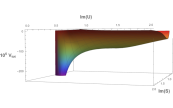
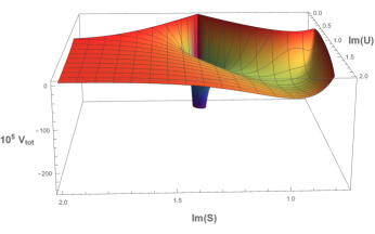
Figure 3: The 3D plot for the anti-de Sitter scalar potential does exhibit a stable minimum. However, after the uplift using a anti-D6-brane this will lead to a runaway.

Unlike for what happens in our working models presented in the main text, finding all masses positive is not an easy task in this setup. Instead, we needed to tune the parameters $a_{S}$ and $b_{S}$ quite a bit. Indeed, this was our reason to include two exponentials: only then were large values for $a_{S}$Im$(S)$ and $b_{S}$Im$(S)$ possible, which is a necessary requirement in order such that higher order non-perturbative corrections can be neglected.

After introducing the uplift, as outlined in section 4, one is unable to find a stable de Sitter vacuum. In figure 3 we show the anti-de Sitter scalar potential before the uplift. After the uplift, in all examples which we studied, this leads to a runaway and no stable de Sitter solution.

References

- (1) S. Kachru, R. Kallosh, A. D. Linde and S. P. Trivedi, De Sitter vacua in string theory, Phys. Rev. D68 (2003) 046005 [hep-th/0301240].
- (2) S. Ferrara, R. Kallosh and A. Linde, Cosmology with Nilpotent Superfields, JHEP 10 (2014) 143 [1408.4096].
- (3) R. Kallosh and T. Wrase, Emergence of Spontaneously Broken Supersymmetry on an Anti-D3-Brane in KKLT dS Vacua, JHEP 12 (2014) 117 [1411.1121].
- (4) E. A. Bergshoeff, K. Dasgupta, R. Kallosh, A. Van Proeyen and T. Wrase, and dS, JHEP 05 (2015) 058 [1502.07627].
- (5) R. Kallosh, F. Quevedo and A. M. Uranga, String Theory Realizations of the Nilpotent Goldstino, JHEP 12 (2015) 039 [1507.07556].
- (6) I. García-Etxebarria, F. Quevedo and R. Valandro, Global String Embeddings for the Nilpotent Goldstino, JHEP 02 (2016) 148 [1512.06926].
- (7) K. Dasgupta, M. Emelin and E. McDonough, Fermions on the antibrane: Higher order interactions and spontaneously broken supersymmetry, Phys. Rev. D95 (2017) 026003 [1601.03409].
- (8) B. Vercnocke and T. Wrase, Constrained superfields from an anti-D3-brane in KKLT, JHEP 08 (2016) 132 [1605.03961].
- (9) R. Kallosh, B. Vercnocke and T. Wrase, String Theory Origin of Constrained Multiplets, JHEP 09 (2016) 063 [1606.09245].
- (10) I. Bandos, M. Heller, S. M. Kuzenko, L. Martucci and D. Sorokin, The Goldstino brane, the constrained superfields and matter in supergravity, JHEP 11 (2016) 109 [1608.05908].
- (11) L. Aalsma, J. P. van der Schaar and B. Vercnocke, Constrained superfields on metastable anti-D3-branes, JHEP 05 (2017) 089 [1703.05771].
- (12) M. P. Garcia del Moral, S. Parameswaran, N. Quiroz and I. Zavala, Anti-D3 branes and moduli in non-linear supergravity, JHEP 10 (2017) 185 [1707.07059].
- (13) N. Cribiori, F. Farakos, M. Tournoy and A. van Proeyen, Fayet-Iliopoulos terms in supergravity without gauged R-symmetry, JHEP 04 (2018) 032 [1712.08601].
- (14) L. Aalsma, M. Tournoy, J. P. Van Der Schaar and B. Vercnocke, Supersymmetric embedding of antibrane polarization, Phys. Rev. D98 (2018) 086019 [1807.03303].
- (15) N. Cribiori, F. Farakos and M. Tournoy, Supersymmetric Born-Infeld actions and new Fayet-Iliopoulos terms, JHEP 03 (2019) 050 [1811.08424].
- (16) N. Cribiori, C. Roupec, T. Wrase and Y. Yamada, Supersymmetric anti-D3-brane action in the Kachru-Kallosh-Linde-Trivedi setup, Phys. Rev. D100 (2019) 066001 [1906.07727].
- (17) Y. Hamada, A. Hebecker, G. Shiu and P. Soler, On brane gaugino condensates in 10d, JHEP 04 (2019) 008 [1812.06097].
- (18) Y. Hamada, A. Hebecker, G. Shiu and P. Soler, Understanding KKLT from a 10d perspective, JHEP 06 (2019) 019 [1902.01410].
- (19) F. Carta, J. Moritz and A. Westphal, Gaugino condensation and small uplifts in KKLT, JHEP 08 (2019) 141 [1902.01412].
- (20) F. F. Gautason, V. Van Hemelryck, T. Van Riet and G. Venken, A 10d view on the KKLT AdS vacuum and uplifting, 1902.01415.
- (21) S. Kachru, M. Kim, L. McAllister and M. Zimet, de Sitter Vacua from Ten Dimensions, 1908.04788.
- (22) T. W. Grimm and J. Louis, The Effective action of type IIA Calabi-Yau orientifolds, Nucl. Phys. B718 (2005) 153 [hep-th/0412277].
- (23) G. Villadoro and F. Zwirner, N=1 effective potential from dual type-IIA D6/O6 orientifolds with general fluxes, JHEP 06 (2005) 047 [hep-th/0503169].
- (24) O. DeWolfe, A. Giryavets, S. Kachru and W. Taylor, Type IIA moduli stabilization, JHEP 07 (2005) 066 [hep-th/0505160].
- (25) P. G. Camara, A. Font and L. E. Ibanez, Fluxes, moduli fixing and MSSM-like vacua in a simple IIA orientifold, JHEP 09 (2005) 013 [hep-th/0506066].
- (26) R. Kallosh and M. Soroush, Issues in type IIA uplifting, JHEP 06 (2007) 041 [hep-th/0612057].
- (27) M. P. Hertzberg, S. Kachru, W. Taylor and M. Tegmark, Inflationary Constraints on Type IIA String Theory, JHEP 12 (2007) 095 [0711.2512].
- (28) S. S. Haque, G. Shiu, B. Underwood and T. Van Riet, Minimal simple de Sitter solutions, Phys. Rev. D79 (2009) 086005 [0810.5328].
- (29) R. Flauger, S. Paban, D. Robbins and T. Wrase, Searching for slow-roll moduli inflation in massive type IIA supergravity with metric fluxes, Phys. Rev. D79 (2009) 086011 [0812.3886].
- (30) U. H. Danielsson, S. S. Haque, G. Shiu and T. Van Riet, Towards Classical de Sitter Solutions in String Theory, JHEP 09 (2009) 114 [0907.2041].
- (31) T. Wrase and M. Zagermann, On Classical de Sitter Vacua in String Theory, Fortsch. Phys. 58 (2010) 906 [1003.0029].
- (32) G. Shiu and Y. Sumitomo, Stability Constraints on Classical de Sitter Vacua, JHEP 09 (2011) 052 [1107.2925].
- (33) D. Junghans, Tachyons in Classical de Sitter Vacua, JHEP 06 (2016) 132 [1603.08939].
- (34) D. Andriot and J. Blaback, Refining the boundaries of the classical de Sitter landscape, JHEP 03 (2017) 102 [1609.00385].
- (35) D. Junghans and M. Zagermann, A Universal Tachyon in Nearly No-scale de Sitter Compactifications, JHEP 07 (2018) 078 [1612.06847].
- (36) D. Andriot, On classical de Sitter and Minkowski solutions with intersecting branes, JHEP 03 (2018) 054 [1710.08886].
- (37) R. Kallosh and T. Wrase, dS Supergravity from 10d, Fortsch. Phys. 2018 (2018) 1800071 [1808.09427].
- (38) V. Balasubramanian, P. Berglund, J. P. Conlon and F. Quevedo, Systematics of moduli stabilisation in Calabi-Yau flux compactifications, JHEP 03 (2005) 007 [hep-th/0502058].
- (39) E. Palti, G. Tasinato and J. Ward, WEAKLY-coupled IIA Flux Compactifications, JHEP 06 (2008) 084 [0804.1248].
- (40) G. Dibitetto, A. Guarino and D. Roest, Charting the landscape of N=4 flux compactifications, JHEP 03 (2011) 137 [1102.0239].
- (41) U. Danielsson and G. Dibitetto, An alternative to anti-branes and O-planes?, JHEP 05 (2014) 013 [1312.5331].
- (42) S. Kachru, R. Kallosh, A. D. Linde, J. M. Maldacena, L. P. McAllister and S. P. Trivedi, Towards inflation in string theory, JCAP 0310 (2003) 013 [hep-th/0308055].
- (43) A. Banlaki, A. Chowdhury, C. Roupec and T. Wrase, Scaling limits of dS vacua and the swampland, JHEP 03 (2019) 065 [1811.07880].
- (44) J. Blaback, U. Danielsson and G. Dibitetto, A new light on the darkest corner of the landscape, 1810.11365.
- (45) A. Retolaza, A. M. Uranga and A. Westphal, Bifid Throats for Axion Monodromy Inflation, JHEP 07 (2015) 099 [1504.02103].
- (46) S. Kachru, J. Kumar and E. Silverstein, Orientifolds, RG flows, and closed string tachyons, Class. Quant. Grav. 17 (2000) 1139 [hep-th/9907038].
- (47) J. J. Blanco-Pillado, C. P. Burgess, J. M. Cline, C. Escoda, M. Gomez-Reino, R. Kallosh et al., Racetrack inflation, JHEP 11 (2004) 063 [hep-th/0406230].
- (48) C. M. Hull and P. K. Townsend, Unity of superstring dualities, Nucl. Phys. B438 (1995) 109 [hep-th/9410167].
- (49) J. H. Schwarz, Lectures on superstring and M theory dualities: Given at ICTP Spring School and at TASI Summer School, Nucl. Phys. Proc. Suppl. 55B (1997) 1 [hep-th/9607201].
- (50) K. Behrndt, R. Kallosh, J. Rahmfeld, M. Shmakova and W. K. Wong, STU black holes and string triality, Phys. Rev. D54 (1996) 6293 [hep-th/9608059].
- (51) B. S. Acharya, K. Bobkov, G. L. Kane, P. Kumar and J. Shao, Explaining the Electroweak Scale and Stabilizing Moduli in M Theory, Phys. Rev. D76 (2007) 126010 [hep-th/0701034].
- (52) E. Witten, Nonperturbative superpotentials in string theory, Nucl. Phys. B474 (1996) 343 [hep-th/9604030].
- (53) H. Looyestijn and S. Vandoren, On NS5-brane instantons and volume stabilization, JHEP 04 (2008) 024 [0801.3949].
- (54) K. Becker, M. Becker and A. Strominger, Five-branes, membranes and nonperturbative string theory, Nucl. Phys. B456 (1995) 130 [hep-th/9507158].
- (55) S. B. Giddings and A. Strominger, STRING WORMHOLES, Phys. Lett. B230 (1989) 46.
- (56) S. Kachru, S. H. Katz, A. E. Lawrence and J. McGreevy, Open string instantons and superpotentials, Phys. Rev. D62 (2000) 026001 [hep-th/9912151].
- (57) R. Blumenhagen, M. Cvetic, S. Kachru and T. Weigand, D-Brane Instantons in Type II Orientifolds, Ann. Rev. Nucl. Part. Sci. 59 (2009) 269 [0902.3251].
- (58) R. Kallosh and A. D. Linde, Landscape, the scale of SUSY breaking, and inflation, JHEP 12 (2004) 004 [hep-th/0411011].
- (59) S. Ferrara and R. Kallosh, Seven-disk manifold, -attractors, and modes, Phys. Rev. D94 (2016) 126015 [1610.04163].
- (60) R. Kallosh, A. Linde, T. Wrase and Y. Yamada, Maximal Supersymmetry and B-Mode Targets, JHEP 04 (2017) 144 [1704.04829].
- (61) S. B. Giddings, S. Kachru and J. Polchinski, Hierarchies from fluxes in string compactifications, Phys. Rev. D66 (2002) 106006 [hep-th/0105097].
- (62) S. Kachru, M. B. Schulz, P. K. Tripathy and S. P. Trivedi, New supersymmetric string compactifications, JHEP 03 (2003) 061 [hep-th/0211182].
- (63) M. Grana, R. Minasian, M. Petrini and A. Tomasiello, A Scan for new N=1 vacua on twisted tori, JHEP 05 (2007) 031 [hep-th/0609124].
- (64) S. Andriolo, G. Shiu, H. Triendl, T. Van Riet, G. Venken and G. Zoccarato, Compact G2 holonomy spaces from SU(3) structures, JHEP 03 (2019) 059 [1811.00063].
- (65) F. Marchesano and J. Quirant, A Landscape of AdS Flux Vacua, 1908.11386.