Induced Spins from Scattering Experiments of Initially Nonspinning Black Holes

Abstract

When two relativistically boosted, nonspinning black holes pass by one another on a scattering trajectory, we might expect the tidal interaction to spin up each black hole. We present the first exploration of this effect, appearing at fourth post-Newtonian order, with full numerical relativity calculations. The basic setup for the calculations involves two free parameters: the initial boost of each black hole and the initial angle between the velocity vectors and a line connecting the centers of the black holes, with zero angle corresponding to a head-on trajectory. To minimize gauge effects, we measure final spins only if the black holes reach a final separation of at least $20M$. Fixing the initial boost, we find that as the initial angle decreases toward the scattering/nonscattering limit, the spin-up grows nonlinearly. In addition, as initial boosts are increased from $0.42c$ to $0.78c$, the largest observed final dimensionless spin on each black hole increases nonlinearly from $0.02$ to $0.20$. Based on these results, we conclude that much higher spin-ups may be possible with larger boosts, although achieving this will require improved numerical techniques.

I Introduction

Inelastic scattering experiments in high-energy physics have deepened our understanding of nonlinear interactions between quarks within hadrons and mesons Bloom et al. (1969); Breidenbach et al. (1969). Analogously, we would expect black hole scattering experiments performed in full numerical relativity to provide insights into strong-field gravity at its strongest and most dynamical. This paper presents such experiments set up in a way that effectively eliminates gauge ambiguities. Specifically, we will address to what degree two relativistically boosted, equal-mass, nonspinning black holes on a scattering trajectory induce spins on each other.

The notion that a black hole’s spin may be influenced by a distant object is not a new one; for example in 1974, Hartle Hartle (1974) demonstrated with analytical arguments that a stationary, coplanar moon far from a spinning black hole will act to spin down the hole. More relevant to our work, a similar effect was studied by Campanelli, Lousto, and Zlochower for black hole binaries in quasicircular orbits Campanelli et al. (2006). They also derived a formula for the radiated angular momentum based on the Weyl scalar $\psi_{4}$ Lousto and Zlochower (2007). However, our work focuses on scattering systems.

Our experimental technique is as follows. We first uniquely specify initial black hole trajectories with Brandt-Brügmann initial data parameters, then perform scattering experiments in full numerical relativity, and finally measure the final black hole spins at large separations. Final spins are measured with both the isolated horizon formalism Ashtekar and Krishnan (2004) and the Christodoulou formula (involving the ratio of proper equatorial to polar circumferences of the apparent horizons) Alcubierre et al. (2005).

The final spins encode important information about the strong-field interaction, which first appears at fourth order in a post-Newtonian expansion in terms that account for the flux of angular momentum at the event horizon Poisson and Sasaki (1995). This work therefore describes a potential way to validate post-Newtonian calculations at very high order with numerical relativity.

Although this work appears to be the first to focus on the final spin of scattering black hole encounters, it is not the first to explore black holes on highly eccentric or hyperbolic trajectories. In one class of such interactions, orbits undergo “zooms” and “whirls”—that is, they whirl close to each other before zooming out to a larger separation, in an extreme example of the precession of the peribothron that occurs near the separatrix of bound and unbound orbits. This class of orbits has been studied in stationary black hole spacetimes Chandrasekhar (2002); Martel (2004); Levin and Perez-Giz (2008), in the post-Newtonian limit Grossman and Levin (2009); Levin and Grossman (2009), and in extreme-mass-ratio systems  Glampedakis and Kennefick (2002); Drasco and Hughes (2006); Haas (2007); Hughes et al. (2005), and is related to the homoclinic orbits observed in stationary black hole spacetimes Bombelli and Calzetta (1992) and in the post-Newtonian limit Cornish and Levin (2003). Khurana and Pretorius were the first to show evidence of zoom-whirl orbits in full numerical relativity, for equal-mass, nonspinning binaries. They simulated up to five zoom-whirls, but showed that many more may be possible, since the number of orbits exhibits critical phenomenon behavior, with exponential scaling in the number of orbits $n$ with the critical impact parameter $b^{*}$: $e^{n}\propto|b-b^{*}|^{\gamma}$ Pretorius and Khurana (2007). Although Khurana and Pretorius fine-tuned their initial data in an attempt to maximize the number of zoom-whirls, Healy, Levin, and Shoemaker found up to three orbits without fine-tuning Healy et al. (2009).

Other studies of zoom-whirl behavior in equal-mass, nonspinning binaries have been performed (see, e.g., Refs. Gold and Brügmann (2013, 2010). These trajectories have also been studied for comparable-mass Kerr black holes Grossman and Levin (2009) and large-mass-ratio Kerr black holes Levin et al. (2011), as well as for binary systems that contain one spinning black hole and one nonspinning black hole Levin and Grossman (2009). Zooms and whirls have even been observed for hyperbolic orbits. Gold and Brügmann showed orbits that exhibited a single whirl followed by a zoom to infinity Gold and Brügmann (2013). Our focus will be on highly eccentric encounters similar to these, with the black holes reaching large separations quickly after a close encounter. Our spin measures assume isolated black holes, so to minimize potential gauge or strong-field effects on these measurements, we only present final spin measures if, after a strong-field encounter, the final separation of the black holes remains at least $20M$ through the end of the calculation; we refer to encounters that satisfy this requirement as “scattering” events, whereas all other encounters are referred to as “nonscattering” or “merger” events. Throughout this work, we will work in geometrized units where $G=c=1$.

Figure 1: Schematic of the chosen initial black hole configuration. $|\vec{p}|$ is the magnitude of the Brandt-Brügmann momentum, $\theta$ is the shooting angle formed with the $x$ axis, and $d$ is the initial orbital separation. For calculations presented here, we choose $d=100$ in code units, corresponding to initial separations between $52.4M$ in the case of an initial $v=0.77$ boost and $96.6M$ in the case of an initial $v=0.42$ boost ($c=1$ units; $M$ is the initial ADM mass), as summarized in Table 2.

As illustrated in Fig. 1, our experimental setup is quite similar to those adopted in the zoom-whirl literature for equal-mass black holes Pretorius and Khurana (2007); Healy et al. (2009); Gold and Brügmann (2013, 2010), with the key exception that we start with a much larger separation of $100$ in code units. This translates to between 50$M$ separation with the highest boosts chosen up to 96$M$ separation with the smallest initial boost, as the initial Arnowitt-Deser-Misner (ADM) mass increases monotonically with the initial boost. The actual values are summarized in Table 2. We find the choice of large initial separations to be especially important, as it gives the gauge fields ample time to settle and enables junk radiation to propagate away so that the gravitational-wave signal due to the dynamical interaction can be analyzed.

At fixed Brandt-Brügmann momentum magnitude $|\vec{p}|$, we find the induced spin-up increases monotonically as $\theta$ decreases toward the scattering/nonscattering separatrix. In addition, the maximum measured spin-up is found to be 0.02, 0.06, 0.11, and 0.20 with initial boosts of $v=0.42$, 0.56, 0.66, and 0.78, respectively. This represents a significantly nonlinear trend as the initial boost parameter is increased. While the induced spins may not seem particularly large for astrophysically motivated boosts such as those potentially seen in hierarchical triple systems, we note that for bound systems, even small induced spins in each encounter may accumulate and significantly impact the dynamics over many orbital time scales.

The rest of the paper is organized as follows: Sec. II discusses the methods used for both the simulations and data analysis; Sec. III describes the initial conditions of each simulation; Sec. IV presents our results; and Sec. V contains our conclusions and plans for future work.

II Numerical Approach and Diagnostics

We adopt standard moving puncture techniques, combining the 3+1 Baumgarte-Shapiro-Shibata-Nakamura (BSSN) formalism Shibata and Nakamura (1995); Baumgarte and Shapiro (1999) with moving puncture gauge conditions to construct the spacetime. We choose $W=e^{-2\phi}$ as our evolved conformal variable, and standard 1+log lapse and Gamma-driver shift conditions.

Initial data are set up and evolutions performed using open-source tools within the Einstein Toolkit (ETK) Löffler et al. (2012); Ein infrastructure. In particular, constraint-satisfying Brandt-Brügmann two-black-hole initial data are generated using the TwoPunctures module Ansorg et al. (2004) with optimized spectral interpolation Paschalidis et al. (2013). The evolution of the BSSN equations was performed with the McLachlan Brown et al. (2009); Kranc ; McLachlan module. QuasiLocalMeasures was applied to calculate black hole spins Dreyer et al. (2003), AHFinderDirect to measure horizon centroids and circumferences Thornburg (2004, 1996), WeylScal4 to compute $\Psi_{4}$ Zilhão and Löffler (2013), as well as the Cactus Computational Toolkit Goodale et al. (2003); Cac ; Cactus developers and Carpet Schnetter et al. (2004); Car for the adaptive mesh refinement grid infrastructure.

II.1 AMR Grid Structure

The adaptive-mesh-refinement (AMR) grids generated by Carpet use half-side lengths of $0.75\times 2^{n}$, for $n=\{0,\ldots,6\},\{8,\ldots,10\}$ in code units. The skip between $n=6$ and $n=8$ ensures a large region within which gravitational waves can be extracted at uniform resolution. All simulations enforce reflection symmetry across the orbital plane to minimize computational expense. The outermost boundary has a half-side length of 768, which ensures that approximate outer boundary conditions can have no causal impact on the spin measures. The three resolutions used for the most refined grid are $\Delta x=\{1/56,1/66.\overline{6},1/85.\overline{3}\};$ henceforth, these shall be referred to as low, medium, and high resolution, respectively. Note that these resolutions are also given in code units, so that higher-boost cases will have higher resolutions (the initial ADM mass $M$ for each boost is given in code units in Table 1). For boosts other than $0.66$, only the “low” resolution was used. Finally, the Carpet parameter time_refinement_factors, which controls how often a time step is performed on each refinement level, is set to [1,1,1,1,2,4,8,16,32,64], so that the coarsest four grids are updated at the same rate, and each refinement level finer than that is updated twice as often as the next-coarser grid. This minimizes interpolation errors on the coarsest levels by disabling time prolongation between them.

II.2 Dimensionless Spin

The dimensionless spin of each black hole, $a/M$, is calculated using two approaches. First is the Christodolou spin, which is given by solving Eq. 5.2 of Ref. Alcubierre et al. (2005),

$$C_{r}=\frac{1+\sqrt{1-(a/M)^{2}}}{\pi}E\left(-\frac{(a/M)^{2}}{\left(1+\sqrt{1-(a/M)^{2}}\right)^{2}}\right),$$ (1)

where $C_{r}=C_{p}/C_{e}$ is the ratio of the polar and equatorial horizon circumferences, and $E(x)$ is the complete elliptic integral of the second kind,

$$E(k)=\int_{0}^{\pi/2}\sqrt{1-k\sin^{2}\theta}d\theta.$$ (2)

Second, the isolated horizon formulation is adopted as an alternative spin measure, which is provided by the ETK QuasiLocalMeasures module.

We also employ standard numerical surface integrals for evaluating the ADM mass $M_{\rm ADM}$ and angular momentum $J_{\rm ADM}$ in the Cartesian basis to measure mass and angular momentum lost to gravitational waves and spin-ups. Additionally, we define the “final angular momentum” and “final spin” to be a time average over the values of angular momentum and spin after the black holes have reached the cutoff separation $r_{\rm cutoff}=20M$ as they move away from each other after the encounter.

$|\vec{p}|$	$M_{\rm ADM}$	SDA @ $\tilde{r}_{\rm cutoff}=5.0$	SDA @ $\tilde{r}_{\rm cutoff}=10.0$	SDA @ $\tilde{r}_{\rm cutoff}=15.0$	SDA @ $\tilde{r}_{\rm cutoff}=20.0$	Maximum $\tilde{r}_{\rm merge}$
$0.490$	1.13560	3.6 (3.4)	4.4 (3.7)	4.6 (3.7)	— (3.8)	3.41
$0.735$	1.28385	3.8 (3.8)	4.5 (4.0)	5.0 (4.1)	— (4.2)	3.95
$0.980$	1.46473	3.7 (3.8)	4.4 (4.1)	4.9 (4.5)	— (4.5)	4.36
$1.500$	1.90902	3.8 (4.0)	4.8 (4.4)	5.6 (4.7)	— (4.7)	3.75

Table 1: Validation of $r_{\rm cutoff}$ choice. Larger choices of $r_{\rm cutoff}$ ensure that the black holes are sufficiently far apart for an accurate final spin measurement and that they are unlikely to merge. The columns are described as follows. $|\vec{p}|$ is the Brandt-Brügmann initial momentum’s magnitude, and $M_{\rm ADM}$ is the initial ADM mass in code units. The next four columns give the mean number of significant digits of agreement (SDA) between the Christodolou spin calculated with that cutoff radius and the Christodolou spin calculated with $r_{\rm cutoff}=20.0M_{\rm ADM}$; the em dashes in the $\tilde{r}_{\rm cutoff}=20.0$ column indicate that the SDA between a measurement and itself is not meaningful. In parentheses, we give the mean SDA between the Christodolou and isolated horizon formalism dimensionless spin measures at points closest to the listed cutoff separation. For brevity we define tilded $r$ quantities in this table to be normalized by $M_{\rm ADM}$; e.g., $\tilde{r}_{\rm cutoff}=r_{\rm cutoff}/M_{\rm ADM}$. Finally, “Maximum $\tilde{r}_{\rm merge}$” is the maximum separation observed between the two holes for cases in which, after a strong-field encounter, they ultimately merged at the given boost.

Our measures of the final spin parameter assume that each black hole is far from another strong-field source and generally on an unbound trajectory. To confirm that our black hole spin measures are reliable, we only include cases in which the holes reach a final separation of at least $r_{\rm cutoff}$ through the end of the calculation. In Table 1, we compare the agreement of Christodolou spins calculated with different cutoff radii with the spin calculated at our chosen $r_{\rm cutoff}=20M$; we see good agreement between cutoffs of $15M$ and $20M$, showing that we have a stable spin measurement. We also compare the Christodolou spin and the isolated horizon formalism measures of spin with varying choices of $r_{\rm cutoff}$, recording at each $r_{\rm cutoff}$ and for each initial boost the significant digits of agreement between the two spin measures (these are the values in parentheses in Table 1). The table confirms that at our fiducial $r_{\rm cutoff}=20M$, the independent black hole spin measures agree to better than four significant digits across most cases. As a point of comparison, we find that over all chosen boost magnitudes and angles, no black holes return to merge after reaching about $r=5M$ separation.

II.3 Parametrizing the Initial Boost

The initial Brandt-Brügmann boost parameter $\vec{p}_{\rm BB}/m_{\rm BB}$ provides an unambiguous measure of the initial boost of each black hole. However, we would expect that the junk radiation associated with the assumption of conformal flatness in Brandt-Brügmann initial data increases as this momentum increases, acting to reduce the momentum of each black hole prior to the interaction more and more as we increase the initial boost Ruchlin et al. (2017).

To parametrize our runs in a way that is insensitive to the presence of junk radiation, we define the initial boost to be the coordinate speed of a single black hole imparted with the same initial Brandt-Brügmann momentum, in the limit $t\to\infty$. In particular, at each initial momentum chosen, we perform a dedicated numerical relativity calculation of a single black hole with this initial momentum, traveling along the $x$ axis. We choose the AMR grids to be identical to the low-resolution experiments, except instead of two AMR grid hierarchies tracking one black hole each, we only need a single hierarchy to track the single black hole.

Plotting the position of the black hole in this calculation versus time, we find that it starts from near zero speed (due to the initial shift $\beta^{i}$ being zero) and accelerates towards some constant speed. However, attempts at a linear fit to the late-time data revealed that the black hole coordinate acceleration on the numerical grids was still nonzero at the end of the calculation, when we were forced to terminate to ensure a valid AMR hierarchy. Therefore, instead of fitting the speed at the end of the calculation, we consider model functions that have asymptotes so the entire time series can be used to estimate the speed that our initial conditions represent.

A hyperbola in the $x$-$t$ plane is a convenient choice here, so we fit hyperbolae to the data by minimizing the residual norm cost function

$$f(a,b,h,k)=\sqrt{\sum_{i=1}^{N}\left(x_{i}-g(a,b,h,k,t_{i})\right)^{2}},$$

where $x_{i}$ and $t_{i}$ are the position and time of the black hole at each of $N$ measurements of position, respectively. $g(a,b,h,k,t)$ is the hyperbola

$$g(a,b,h,k,t)=k-\sqrt{a^{2}\left(1+\frac{(t-h)^{2}}{b^{2}}\right)},$$

where $a$ is the semimajor axis, $b$ is the semiminor axis, and $(h,k)$ are the coordinates of the center. We then take the slope of the asymptote $a/b$ as the actual preinteraction boost that corresponds to the input momentum. As illustrated in Fig. 2, the hyperbolic fit to data plotted at these late times is quite good.

This hyperbolic fitting method produces values of $v=0.42$, 0.56, 0.66, and 0.78, corresponding to magnitudes of the initial Brandt-Brügmann momentum of $|\vec{p}|=0.49$, 0.735, 0.98, and 1.50, respectively. Interestingly, these estimates for the initial boost are quite close to the respective values of $|\vec{p}|/M_{\rm ADM}=0.43$, 0.57, 0.67, and 0.79. Notice however that our measured asymptotic coordinate boost is always slightly lower than the Brandt-Brügmann momentum-based measure, presumably due to the emission of junk radiation.

Figure 2: Parametrizing the initial boost: Late-time data of dedicated single-black-hole runs to find the initial boost. Here, $t=0$ corresponds to an arbitrarily chosen later time, and all of these boost calibration calculations were performed to a final time of $\approx 250M$. The dashed lines show the asymptotic slope, solid lines show the actual data from the numerical relativity calculation, and the points show the hyperbolic fit.

II.4 Radiated Angular Momentum

As the black holes are initially nonspinning, the orbital angular momentum contributes the entirety of the system’s initial angular momentum. As the numerical relativity calculation progresses, however, this orbital contribution decreases as the black holes are spun up and gravitational waves carry away angular momentum. The radiated angular momentum $J_{\rm GW}$ is calculated using

$$J_{\rm GW}=\frac{r^{2}_{\rm ext}}{16\pi}\sum_{l,m}\int_{-\infty}^{t}-m(\dot{h}_{+}h_{\times}-\dot{h}_{\times}h_{+})dt,$$ (3)

derived from Eq. 24 of Ref. Campanelli and Lousto (1999). In all cases we measure the strain from the outgoing Weyl scalar $\psi_{4}$ at $r_{\rm ext}=67.88M$, which is sufficiently far from the binary but in a high-enough resolution region to yield a reliable result.

III Initial Conditions

For all sets of simulations, the initial separation was set to $d=100$. Such large initial separations allow more time for the junk-radiation-induced perturbation on each black hole to settle before the holes strongly interact, and ensure that a sufficient interval of time exists between the junk and the gravitational radiation from the dynamical interaction.

In a given simulation with $|\vec{p}|$ and $\theta$ (whether bound or unbound), we set $p_{x}=\pm|\vec{p}|\cos(\theta)$ and $p_{y}=\mp|\vec{p}|\sin(\theta)$, giving rise to the configuration shown in Fig. 1 (this figure is not to scale).

Boost ($v$)	$|\vec{p}|$	Resolution	$d/M_{\rm ADM}$	$\theta_{\rm N-S}$	$N_{\theta_{\rm N-S}}$	$\theta_{\rm S}$	$N_{\theta_{\rm S}}$
$0.42$	$0.490$	Low	96.6	$\{5.600\times 10^{-2},6.040\times 10^{-2}\}$	$11$	$\{6.050\times 10^{-2},7.100\times 10^{-2}\}$	$23$
$0.56$	$0.735$	Low	77.9	$\{5.400\times 10^{-2},5.440\times 10^{-2}\}$	$3$	$\{5.460\times 10^{-2},6.500\times 10^{-2}\}$	$31$
$0.66$	$0.980$	Low	68.2	$\{5.400\times 10^{-2},5.420\times 10^{-2}\}$	$3$	$\{5.430\times 10^{-2},5.800\times 10^{-2}\}$	$28$
$0.66$	$0.980$	Medium	68.2	$\{5.400\times 10^{-2},5.420\times 10^{-2}\}$	$3$	$\{5.430\times 10^{-2},5.800\times 10^{-2}\}$	$28$
$0.66$	$0.980$	High	68.2	$\{5.418\times 10^{-2},5.424\times 10^{-2}\}$	$3$	$\{5.430\times 10^{-2},5.690\times 10^{-2}\}$	$17$
$0.77$	$1.500$	Low	52.4	$\{3.000\times 10^{-2},5.950\times 10^{-2}\}$	$9$	$\{5.960\times 10^{-2},7.000\times 10^{-2}\}$	$21$

Table 2: Initial conditions for black hole scattering experiments. $|\vec{p}|$ is the magnitude of the initial Brandt-Brügmann momentum; $\theta_{\rm N-S}$ and $\theta_{\rm S}$ are the ranges of the initial shooting angles (in radians) of the Brandt-Brügmann momentum for cases exhibiting scattering and nonscattering (“merging”) behavior, respectively; and $N_{\theta_{\rm N-S}}$ and $N_{\theta_{\rm S}}$ are the number of simulations in those ranges.

Table 2 presents a complete list of calculations performed in this work. Notice that runs for $|\vec{p}|=0.980$ were carried out at three different resolutions, with grids as specified in Sec. II.1. Upon finding that results (i.e., final measured spin parameters) were not significantly improved at higher resolutions, other runs were carried out at low resolution.

The range of angles (given in radians) and number of runs performed in each set of experiments are also given; these sets are divided into subsets corresponding to bound and unbound trajectories. For instance, when setting the momentum magnitude to $0.490$, we find that the initial boost is $v=0.42$ and that the angle $\theta=6.050\times 10^{-2}$ marks the boundary between scattering and nonscattering (i.e. “merging”) cases. We performed 23 simulations between that angle and $\theta=7.100\times 10^{-2}$ and an additional 11 simulations satisfying $5.600\times 10^{-2}\leq\theta\leq 6.040\times 10^{-2}$ as we searched for the transition between scattering and nonscattering trajectories. Note that the separatrix angle between scattering/nonscattering is not monotonic in boost; this happens because the fixed initial separation in code units $d$ combined with the larger initial ADM mass $M$ in the higher-boost cases decreases the initial dimensionless separation $d/M$, so the angles are not immediately comparable.

IV Results

IV.1 Trajectory Morphologies

The chosen set of initial conditions results in a variety of scattering and nonscattering (i.e. “merging”) trajectories, as shown in Fig. 3. It is clear from the plots that this strong-field scattering exhibits much richer morphology than its classical analogue; some trajectories are zoom-whirl-like, as can be seen in the left and middle plots in Fig. 3. Likewise, while the right panel does not show a true “zoom,” it is far from Keplerian due to the emission of gravitational waves and black hole spin-ups.

The plots of Fig. 3 also relate to how initial conditions are chosen: we first selected four Brandt-Brügmann momenta magnitudes corresponding to initial boosts of $v\approx 0.42,0.56,0.66,$ and $0.78$ (as measured in Sec. II.3). At each of these magnitudes, we reduced the shooting angle until immediate merger occurred. This resulted in three classes of trajectories: immediate mergers (not of interest to this study), marginal scattering (which may subsequently merge, but the holes remain isolated long enough for a reliable spin measurement), and scattering; these are illustrated in the left, middle, and right plots in Fig. 3, respectively.

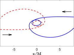
Figure 3: Nonscattering (left), marginally scattered (middle), and scattered (right) black hole trajectories. Arrows indicate the direction each puncture is initially traveling and $M$ is the initial ADM mass of the system.

IV.2 $v_{\rm boost}=0.66$ Spin-Up Study

The left panel of Fig. 4 presents final spin data from the $v_{\rm boost}=0.66$ case carried out at three resolutions. As can be seen, spin-up occurs in every case, and measures at different numerical resolutions agree well with each other: the relative error between spins at medium and low resolution never exceeds 1.4%, and the relative error between high- and medium-resolution spins never exceeds 0.6%. Comparing the Christodolou and the isolated horizon formalism Ashtekar and Krishnan (2004) measures of dimensionless spin $J/M^{2}$ for each hole, we find agreement to within one percent in the worst case; typically the two measures agree to three to five significant digits.

The spin-up increases as the shooting angle decreases towards the separatrix between scattering and nonscattering trajectories. This increase is nonlinear and concave-up, reaching a maximum of $0.11$ .

Figure 4: Left panel: The final spin $a/M$ is computed by averaging the Christodoulou spin over late times (once the black holes are sufficiently far apart as to be weakly interacting, which we have defined as $20M$ separation), and is here plotted against the shooting angle $\theta$, which increases with impact parameter.
Right panel: The maximum spin-up obtained at a given initial boost is plotted using open circles; the error bars on these points do not exceed $10\%$ of the point’s value. Other spin-ups are displayed as points; thus, the shooting angle increases downwards on this plot for a given set of points. The shaded region above the dashed line indicates the regime of immediate mergers. Black arrows on this plot indicate the direction of decreasing $\theta$.

IV.3 Maximum Spin-Up

Expanding our analysis to the other boost cases, we again find that in scattering cases, as the separatrix is approached, the spin-up increases to its maximum. This study provides the additional insight that the maximum spin-up depends strongly on the initial boost, as shown in the right panel of Fig. 4. As we increase the initial boost of the BHs, the maximum final BH spin obtainable at that boost increases; again, this increase is significant and nonlinear. The maximum spin for $v=0.42$ was $0.02$, and for $v=0.56$, we found $0.06$. The maximum induced spin parameter we found overall was $0.20$, for $v=0.78$.

As we demonstrated previously, the spin measures are quite reliable, and in fact the largest uncertainty in maximum induced spin at a given initial boost comes from whether or not we truly found the shooting angle closest to an immediate merger. Therefore, in Fig. 4, we base the error bars on sampling resolution in shooting angle. (The error bars are similar in size to the open circles, and become difficult to distinguish for some of the points.) The error bars in the right panel of Fig. 4 are calculated as the difference between the highest and second-highest spin measured at a given boost. Again, the error bars are smaller than the data points themselves.

IV.4 Spin-Up Efficiency

Figure 5: Spin-up efficiency, measured as the fraction of the initial angular momentum, $J_{0}$, that was transferred to the spins of the two black holes, $2J_{\rm BH}$.

The angular momentum spinning up the holes originates from the orbital angular momentum in the initial data. We would like to identify what fraction of this initial angular momentum is transferred into spin angular momentum. Figure 5 plots the efficiency of spin-up, $2J_{\rm BH}/J_{0}$, and the proportion of orbital angular momentum remaining in the system after the encounter, $J_{\rm final}=(J_{0}-J_{\rm GW}-2J_{\rm BH})/J_{0}$. Here, we define $J_{\rm BH}$ to be the dimensionful angular momentum as calculated using the isolated horizon formalism, and $J_{\rm GW}$ is defined in Eq. 3.

Fixing the initial boost, the smallest angle resulting in a scattering trajectory corresponds to the largest $J_{\rm BH}$ and, therefore, the largest spin-up efficiency. Further, we find that higher boosts increase the spin-up efficiency as well. We conclude that this spin-up effect has the potential to significantly impact the orbital evolution of a binary. This is not taken into account in current, commonly used post-Newtonian (PN) approximants, as the spin-up is not modeled until 4PN order Poisson and Sasaki (1995). Further, adding spin-spin and spin-orbit interaction terms to initially nonspinning configurations is not yet a standard approach in PN. Adding such terms would be necessary to use these results to validate PN theory.

V Conclusions

We found that decreasing the shooting angle at a given initial boost increases the spin induced onto black holes that undergo a scattering trajectory. Further, as the initial boost is increased, the maximum spin-up and spin-up efficiency (i.e. the fraction of the initial angular momentum transferred to the black holes’ spins) increases nonlinearly.

The maximum spin-up observed was $a/M=0.20$ imparted on each hole, which occurs with an initial boost of $0.78c$ (the maximum boost chosen). This also corresponds to the maximum spin-up efficiency observed, of $2J_{BH}/J_{0}=3.9\%$. Once post-Newtonian theory has been completed at 4PN order for this type of interaction, this work will provide an exciting new avenue for validating PN theory directly with numerical relativity calculations.

These results indicate that the spin-ups and spin-up efficiencies may increase significantly with larger initial boosts, which will be a focus of future work. However, this work presents boosts near the upper limit allowed by conformally flat Brandt-Brügmann initial data, so larger initial boosts will require improved initial data a la Ruchlin, Healy, Lousto, and Zlochower Ruchlin et al. (2017), as well as higher numerical resolutions.

This is a very rich problem with a massive parameter space left to explore, and we hope to eventually study cases with varying initial spins and unequal mass ratios. With so many options available, we plan to add black hole scattering experiments to BlackHoles@Home, a distributed computing project enabling numerical relativity calculations of black hole interactions to be performed on consumer-grade desktop or laptop computers Ruchlin et al. (2018); Etienne and Ruchlin (2018); Ruchlin et al. (2018).

In future work we would also like to extract more gauge-invariant quantities from the gravitational-wave data, such as the peak frequency of the radiation, $f_{\rm peak}$. We attempted to do so with these data, but they were too noisy to obtain reliable measures. It would also be useful as an additional validation to measure the conservation of total $J$ in the system by, e.g., directly computing the ADM $J_{\rm final}$ and comparing it to the proxy $J_{0}-J_{\rm GW}-2J_{\rm BH}$ that we used. Verifying conservation of total $M_{\rm ADM}$ will be useful as well.

More broadly speaking, we hope that the calculations performed here will allow us to characterize a subtle strong-field effect that could nonetheless bring about observable effects in future high-precision gravitational-wave observations.

References

- Bloom et al. (1969) E. D. Bloom, D. H. Coward, H. DeStaebler, J. Drees, G. Miller, L. W. Mo, R. E. Taylor, M. Breidenbach, J. I. Friedman, G. C. Hartmann, and H. W. Kendall, Phys. Rev. Lett. 23, 930 (1969).
- Breidenbach et al. (1969) M. Breidenbach, J. I. Friedman, H. W. Kendall, E. D. Bloom, D. H. Coward, H. DeStaebler, J. Drees, L. W. Mo, and R. E. Taylor, Phys. Rev. Lett. 23, 935 (1969).
- Hartle (1974) J. B. Hartle, Phys. Rev. D 9, 2749 (1974).
- Campanelli et al. (2006) M. Campanelli, C. O. Lousto, and Y. Zlochower, Phys. Rev. D 74, 084023 (2006), astro-ph/0608275 .
- Lousto and Zlochower (2007) C. O. Lousto and Y. Zlochower, Phys. Rev. D76, 041502 (2007), arXiv:gr-qc/0703061 [gr-qc] .
- Ashtekar and Krishnan (2004) A. Ashtekar and B. Krishnan, Living Reviews in Relativity 7 (2004), 10.12942/lrr-2004-10, gr-qc/0407042 .
- Alcubierre et al. (2005) M. Alcubierre et al., Phys. Rev. D72, 044004 (2005), arXiv:gr-qc/0411149 [gr-qc] .
- Poisson and Sasaki (1995) E. Poisson and M. Sasaki, Phys. Rev. D51, 5753 (1995), arXiv:gr-qc/9412027 [gr-qc] .
- Chandrasekhar (2002) S. Chandrasekhar, The mathematical theory of black holes, Oxford classic texts in the physical sciences (Oxford Univ. Press, Oxford, 2002).
- Martel (2004) K. Martel, Phys. Rev. D69, 044025 (2004), arXiv:gr-qc/0311017 [gr-qc] .
- Levin and Perez-Giz (2008) J. Levin and G. Perez-Giz, Phys. Rev. D77, 103005 (2008), arXiv:0802.0459 [gr-qc] .
- Grossman and Levin (2009) R. Grossman and J. Levin, Phys. Rev. D 79, 043017 (2009), arXiv:0811.3798 [gr-qc] .
- Levin and Grossman (2009) J. Levin and R. Grossman, Phys. Rev. D 79, 043016 (2009), arXiv:0809.3838 [gr-qc] .
- Glampedakis and Kennefick (2002) K. Glampedakis and D. Kennefick, Phys. Rev. D 66, 044002 (2002), gr-qc/0203086 .
- Drasco and Hughes (2006) S. Drasco and S. A. Hughes, Phys. Rev. D73, 024027 (2006), [Erratum: Phys. Rev.D90,no.10,109905(2014)], arXiv:gr-qc/0509101 [gr-qc] .
- Haas (2007) R. Haas, Phys. Rev. D75, 124011 (2007), arXiv:0704.0797 [gr-qc] .
- Hughes et al. (2005) S. A. Hughes, S. Drasco, E. E. Flanagan, and J. Franklin, Phys. Rev. Lett. 94, 221101 (2005).
- Bombelli and Calzetta (1992) L. Bombelli and E. Calzetta, Classical and Quantum Gravity 9, 2573 (1992).
- Cornish and Levin (2003) N. J. Cornish and J. Levin, Classical and Quantum Gravity 20, 1649 (2003), arXiv:gr-qc/0304056 [gr-qc] .
- Pretorius and Khurana (2007) F. Pretorius and D. Khurana, Classical and Quantum Gravity 24, S83 (2007), gr-qc/0702084 .
- Healy et al. (2009) J. Healy, J. Levin, and D. Shoemaker, Physical Review Letters 103, 131101 (2009), arXiv:0907.0671 [gr-qc] .
- Gold and Brügmann (2013) R. Gold and B. Brügmann, Phys. Rev. D 88, 064051 (2013), arXiv:1209.4085 [gr-qc] .
- Gold and Brügmann (2010) R. Gold and B. Brügmann, Classical and Quantum Gravity 27, 084035 (2010), arXiv:0911.3862 [gr-qc] .
- Levin et al. (2011) J. Levin, S. T. McWilliams, and H. Contreras, Classical and Quantum Gravity 28, 175001 (2011), arXiv:1009.2533 [gr-qc] .
- Gold and Brügmann (2013) R. Gold and B. Brügmann, Phys. Rev. D88, 064051 (2013), arXiv:1209.4085 [gr-qc] .
- Shibata and Nakamura (1995) M. Shibata and T. Nakamura, Phys. Rev. D 52, 5428 (1995).
- Baumgarte and Shapiro (1999) T. W. Baumgarte and S. L. Shapiro, Phys. Rev. D 59, 024007 (1999), gr-qc/9810065 .
- Löffler et al. (2012) F. Löffler, J. Faber, E. Bentivegna, T. Bode, P. Diener, R. Haas, I. Hinder, B. C. Mundim, C. D. Ott, E. Schnetter, G. Allen, M. Campanelli, and P. Laguna, Classical and Quantum Gravity 29, 115001 (2012), arXiv:1111.3344 [gr-qc] .
- (29) “The Einstein Toolkit,” https://einsteintoolkit.org.
- Ansorg et al. (2004) M. Ansorg, B. Brügmann, and W. Tichy, Phys. Rev. D 70, 064011 (2004), gr-qc/0404056 .
- Paschalidis et al. (2013) V. Paschalidis, Z. B. Etienne, R. Gold, and S. L. Shapiro, ArXiv e-prints (2013), arXiv:1304.0457 [gr-qc] .
- Brown et al. (2009) J. D. Brown, P. Diener, O. Sarbach, E. Schnetter, and M. Tiglio, Phys. Rev. D 79, 044023 (2009), arXiv:0809.3533 [gr-qc] .
- (33) Kranc, “Kranc: Kranc assembles numerical code,” http://kranccode.org/.
- (34) McLachlan, “McLachlan, a public BSSN code,” http://www.cct.lsu.edu/~eschnett/McLachlan/.
- Dreyer et al. (2003) O. Dreyer, B. Krishnan, D. Shoemaker, and E. Schnetter, Phys. Rev. D 67, 024018 (2003), gr-qc/0206008 .
- Thornburg (2004) J. Thornburg, Classical and Quantum Gravity 21, 743 (2004), gr-qc/0306056 .
- Thornburg (1996) J. Thornburg, Phys. Rev. D 54, 4899 (1996), arXiv:gr-qc/9508014 .
- Zilhão and Löffler (2013) M. Zilhão and F. Löffler, International Journal of Modern Physics A 28, 1340014-126 (2013), arXiv:1305.5299 [gr-qc] .
- Goodale et al. (2003) T. Goodale, G. Allen, G. Lanfermann, J. Massó, T. Radke, E. Seidel, and J. Shalf, “High Performance Computing for Computational Science — VECPAR 2002: 5th International Conference Porto, Portugal, June 26–28, 2002 Selected Papers and Invited Talks,” (Springer Berlin Heidelberg, Berlin, Heidelberg, 2003) Chap. The Cactus Framework and Toolkit: Design and Applications, pp. 197–227.
- (40) “Cactus computational toolkit,” https://www.cactuscode.org.
- (41) Cactus developers, “Cactus Computational Toolkit Prizes,” http://cactuscode.org/media/prizes/.
- Schnetter et al. (2004) E. Schnetter, S. H. Hawley, and I. Hawke, Classical and Quantum Gravity 21, 1465 (2004), gr-qc/0310042 .
- (43) “Carpet: Adaptive mesh refinement for cactus framework,” https://www.carpetcode.org.
- Ruchlin et al. (2017) I. Ruchlin, J. Healy, C. O. Lousto, and Y. Zlochower, Phys. Rev. D95, 024033 (2017), arXiv:1410.8607 [gr-qc] .
- Campanelli and Lousto (1999) M. Campanelli and C. O. Lousto, Phys. Rev. D 59, 124022 (1999), gr-qc/9811019 .
- Note (1) Note that the shooting angle is related to the impact parameter via , where is the initial separation between the holes. Since the shooting angles we use are small, the small-angle approximation gives , so the left panel of Fig. 4 would remain almost entirely unchanged if the impact parameter were plotted instead of the shooting angle.
- Ruchlin et al. (2018) I. Ruchlin, Z. B. Etienne, and T. W. Baumgarte, Phys. Rev. D97, 064036 (2018), arXiv:1712.07658 [gr-qc] .
- Etienne and Ruchlin (2018) Z. B. Etienne and I. Ruchlin, “NRPy+: Code generator for Numerical Relativity,” Astrophysics Source Code Library (2018), ascl:1807.025 .
- Ruchlin et al. (2018) I. Ruchlin, Z. B. Etienne, and T. W. Baumgarte, “SENR: Simple, Efficient Numerical Relativity,” Astrophysics Source Code Library (2018), ascl:1807.026 .