Graduated Non-Convexity for Robust Spatial Perception:
From Non-Minimal Solvers to Global Outlier Rejection

Abstract

Semidefinite Programming (SDP) and Sums-of-Squ- ares (SOS) relaxations have led to certifiably optimal non-minimal solvers for several robotics and computer vision problems. However, most non-minimal solvers rely on least squares formulations, and, as a result, are brittle against outliers. While a standard approach to regain robustness against outliers is to use robust cost functions, the latter typically introduce other non-convexities, preventing the use of existing non-minimal solvers. In this paper, we enable the simultaneous use of non-minimal solvers and robust estimation by providing a general-purpose approach for robust global estimation, which can be applied to any problem where a non-minimal solver is available for the outlier-free case. To this end, we leverage the Black-Rangarajan duality between robust estimation and outlier processes (which has been traditionally applied to early vision problems), and show that graduated non-convexity (GNC) can be used in conjunction with non-minimal solvers to compute robust solutions, without requiring an initial guess. Although GNC’s global optimality cannot be guaranteed, we demonstrate the empirical robustness of the resulting robust non-minimal solvers in applications, including point cloud and mesh registration, pose graph optimization, and image-based object pose estimation (also called shape alignment). Our solvers are robust to 70-80% of outliers, outperform RANSAC, are more accurate than specialized local solvers, and faster than specialized global solvers. We also propose the first certifiably optimal non-minimal solver for shape alignment using SOS relaxation.

I Introduction

Robust estimation is a crucial tool for robotics and computer vision, being concerned with the estimation of unknown quantities (e.g., the state of a robot, or of variables describing the external world) from noisy and potentially corrupted measurements. Corrupted measurements (i.e., outliers) can be caused by sensor malfunction, but are more commonly associated with incorrect data association and model misspecification [1, 2].

In the outlier-free case, common estimation problems are formulated as a least squares optimization:

$$\min_{{\bm{x}}\in{\cal X}}\;\sum_{i=1}^{N}r^{2}({\bm{y}}_{i},{\bm{x}}),$$ (1)

where ${\bm{x}}$ is the variable we want to estimate (e.g., the pose of an unknown object); ${\cal X}$ is the domain of ${\bm{x}}$ (e.g., the set of 3D poses); ${\bm{y}}_{i}$ ($i=1,\ldots,N$) are given measurements (e.g., pixel observations of points belonging to the object); and the function $r({\bm{y}}_{i},{\bm{x}})$ is the residual error for the $i$-th measurement, quantifying the mismatch between the expected measurement at an estimate ${\bm{x}}$ and the actual measurement ${\bm{y}}_{i}$. In typical robotics and computer vision applications,  the least squares optimization (1) is difficult to solve globally, due to the nonlinearity of the residual errors and the nonconvexity of the domain ${\cal X}$. Despite these challenges, the research community has developed closed-form solutions and globally optimal solvers for many such problems. Specifically, while closed-form solutions are rare [3], Semidefinite Programming (SDP) and Sums-of-Squares (SOS) [4] relaxations have been recently shown to be a powerful tool to obtain certifiably optimal solutions to relevant instances of problem (1), ranging from pose graph optimization [5, 6], rotation averaging [7], anisotropic registration [8], two-view geometry [9], and PnP [10]. The resulting techniques are commonly referred to as non-minimal solvers, to contrast them against methods that solve problem (1) using only a small (minimal) subset of measurements ${\bm{y}}_{i}$ (see related work in Section II).

Unfortunately, in the presence of outliers, problem (1)’s solution provides a poor estimate for ${\bm{x}}$. This limits the applicability of existing non-minimal solvers, since they can be applied only after the outliers have been removed. Yet, the theory of robust estimation suggests regaining robustness by substituting the quadratic cost in the least squares problem (1) with a robust cost $\rho(\cdot)$:

$$\min_{{\bm{x}}\in{\cal X}}\;\sum_{i=1}^{N}\rho(r({\bm{y}}_{i},{\bm{x}})).$$ (2)

For instance, $\rho(\cdot)$ can be a Huber loss, a truncated least squares cost, or a Geman-McClure cost [11]. To date, the application of non-minimal solvers to eq. (2) has been limited. Some of the non-minimal solvers designed for (1) can be extended to include a convex robust cost function, such as the Huber loss [12]; however, it is known that convex losses have a low breakdown point and are still sensitive to gross outliers [13]. In rare cases, the literature provides robust non-minimal solvers that achieve global solutions to specific instances of problem (2), such as robust registration [2, 14]. However, these solvers cannot be easily extended to other estimation problems, and they rely on solving large SDPs, which is currently impractical for large-scale problems.

Contributions. In this paper, we aim to reconcile non-minimal solvers and robust estimation, by providing a general-purpose algorithm to solve problem (2) without requiring an initial guess. We achieve this by combining non-minimal solvers with an approach known as graduated non-convexity (GNC). In contrast, standard algorithms for problem (2) rely on iterative optimization to refine a given initial guess, which causes the result to be brittle when the quality of the guess is poor. Particularly, we propose three contributions.

First, we revisit the Black-Rangarajan duality [11] between robust estimation and outlier processes. We also revisit the use of graduated non-convexity (GNC) as a general tool to solve a non-convex optimization problem without an initial guess. While Black-Rangarajan duality and GNC have been used in early vision problems, such as stereo reconstruction, image restoration and segmentation, and optical flow, we show that combining them with non-minimal solvers allows solving spatial perception problems, ranging from mesh registration, pose graph optimization, and image-based object pose estimation.

Our second contribution is to tailor Black-Rangarajan duality and GNC to the Geman-McClure and truncated least squares costs. We show how to optimize these functions by alternating two steps: a variable update, which solves a weighted least squares problem using non-minimal solvers; and a weight update, which updates the outlier process in closed form.

Our approach requires a non-minimal solver, but currently there is no such solver for image-based object pose estimation (also known as shape alignment). Our third contribution is to present a novel non-minimal solver for shape alignment. While related techniques propose approximate relaxations [15], we provide a certifiably optimal solution using SOS relaxation.

We demonstrate our robust non-minimal solvers on point cloud registration (P-REG), mesh registration (as known as generalized registration, G-REG), pose graph optimization (PGO), and shape alignment (SA). Our solvers are robust to 70-80% outliers, outperform RANSAC, are more accurate than specialized local solvers, and faster than global solvers.

II Related Work

II-A Outlier-free Estimation

Minimal Solvers. Minimal solvers use the smallest number of measurements necessary to estimate ${\bm{x}}$. Examples include the 2-point solver for the Wahba problem (a rotation-only variant of P-REG) [16], the 3-point solver for P-REG [3], and the 12-point solver [17] for G-REG with point-to-plane correspondences. Notably, the approach [18] enables minimal solvers for a growing number of estimation problems.

Non-minimal Solvers. Minimal solvers do not leverage data redundancy, and, consequently, can be sensitive to measurement noise. Therefore, non-minimal solvers have been developed. Typically, non-minimal solvers assume Gaussian measurement noise, which results in a least squares optimization framework. In some cases, the resulting optimization problems can be solved in closed form, e.g., Horn’s method [3] for P-REG, or PLICP [19] for G-REG. Generally, however, the resulting optimization problems are hard and only locally optimal solutions can be obtained [20]. For global optimization, researchers have developed exponential-time methods, such as Branch and Bound (BnB). Hartley and Kahl [21] introduce a BnB search over the rotation space to globally solve several vision problems. Olsson et al. [22] develop optimal solutions for G-REG. Recently, Semidefinite Programing (SDP) and Sums of Squares (SOS) relaxations [4] have been used to develop polynomial-time algorithms with certifiable optimality guarantees. Briales and Gonzalez-Jimenez [8] solve G-REG using SDP. Carlone et al. [5, 23] use Lagrangian duality and SDP relaxations for PGO. Rosen et al. [6] develop SE-Sync, a fast solver for the relaxation in [5, 23]. Mangelson et al. [24] apply the sparse bounded-degree variant of SOS relaxation, also for PGO. Currently, there are no certifiably optimal non-minimal solvers for shape alignment; Zhou et al. [15] propose a convex relaxation to obtain an approximate solution for SA.

II-B Robust Estimation

Global Methods. We refer to a robust method as global, if it does not require an initial guess. Several global methods adopt the framework of consensus maximization [25, 26], which looks for an estimate that maximizes the number of measurements that are explained within a prescribed estimation error. Consensus maximization is NP-hard [25, 27], and related work investigates both approximations and exact algorithms. RANSAC [28] is a widely used heuristic, applicable when a minimal solver exists. But RANSAC provides no optimality guarantees, and its running time grows exponentially with the outlier ratio [29]. Tzoumas et al. [27] develop the general-purpose Adaptive Trimming (ADAPT) algorithm, that has linear running time, and, instead, is applicable when a non-minimal solver exists. Mangelson et al. [30] propose a graph-theoretic method to prune outliers in PGO. Exact solutions for consensus maximization are based on BnB [26]: see [31] for the Wahba problem, and [29] for P-REG.

Another framework for global methods is M-estimation, which resorts to robust cost functions. Enqvist et al. [32] use a truncated least squares (TLS) cost, and propose an approach that scales, however, exponentially with the dimension of the parameter space. More recently, SDP relaxations have also been used to optimize robust costs. Carlone and Calafiore [12] develop convex relaxations for PGO with $\ell_{1}$-norm and Huber loss functions. Lajoie et al. [13] adopt a TLS cost for PGO. Yang and Carlone [2, 14] develop an SDP relaxation for the Wahba and P-REG problem, also adopting a TLS cost. Currently, the poor scalability of the state-of-the-art SDP solvers limits these algorithms to only small-size problems.

Finally, graduated non-convexity (GNC) methods have also been employed to optimize robust costs [33]. Rather than directly optimizing a non-convex robust cost, these methods sequentially optimize a sequence of surrogate functions, which start from a convex approximation of the original cost, but then gradually become non-convex, converging eventually to the original cost. Despite GNC’s success in early computer vision applications [11, 34], its broad applicability has remain limited due to the lack of non-minimal solvers. Indeed, only a few specialized methods for spatial perception have used GNC. Particularly, Zhou et al. [35] develop a method for P-REG, using Horn’s or Arun’s methods [3, 36].

Local Methods. In contrast to global methods, local methods require an initial guess. In the context of M-estimation, these methods iteratively optimize a robust cost function till they converge to a local minimum [37]. Zach et al. [38] include auxiliary variables and propose an iterative optimization approach that alternates updates on the estimates and the auxiliary variables; the approach still requires an initial guess. Bouaziz et al. [39] propose robust variants of the iterative closest point algorithm for P-REG. Sünderhauf and Protzel [40], Olson and Agarwal [41], Agarwal et al. [42], Pfingsthorn and Birk [43] propose local methods for PGO. Wang et al. [44] investigate local methods for shape alignment.

III Black-Rangarajan Duality and Graduated Non-convexity

We review the Black-Rangarajan duality [11], and a tool for global optimization known as graduated non-convexity [33].

III-A Black-Rangarajan Duality

This section revisits the Black-Rangarajan duality between robust estimation and outlier process [11]. This theory is less known in robotics, and its applications have been mostly targeting early vision problems, with few notable exceptions.

Lemma 1 (Black-Rangarajan Duality [11]).

Given a robust cost function $\rho(\cdot)$, define $\phi(z)\doteq\rho(\sqrt{z})$. If $\phi(z)$ satisfies $\lim_{z\rightarrow 0}\phi^{\prime}(z)=1$, $\lim_{z\rightarrow\infty}\phi^{\prime}(z)=0$, and $\phi^{\prime\prime}(z)<0$, then the robust estimation problem (2) is equivalent to

$$\min_{{\bm{x}}\in{\cal X},w_{i}\in[0,1]}\sum_{i=1}^{N}\left[w_{i}r^{2}({\bm{y}}_{i},{\bm{x}})+\Phi_{\rho}(w_{i})\right],$$ (3)

where $w_{i}\in[0,1]$ ($i=1,\dots,N$) are slack variables (or weights) associated to each measurement ${\bm{y}}_{i}$, and the function $\Phi_{\rho}(w_{i})$ (the so called outlier process) defines a penalty on the weight $w_{i}$. The expression of $\Phi_{\rho}(w_{i})$ depends on the choice of robust cost function $\rho(\cdot)$.

The conditions on $\rho(\cdot)$ are satisfied by all common choices of robust costs [11]. Besides presenting this fundamental result, asserting the equivalence between the outlier process (3) and the robust estimation (2), Black and Rangarajan provide a procedure (see Fig. 10 in [11]) to compute $\Phi_{\rho}(w_{i})$ and show that common robust cost functions admit a simple analytical expression for $\Phi_{\rho}(w_{i})$. Interestingly, the outlier process (3) has been often used in robotics and SLAM [42, 40], without acknowledging the connection with robust estimation, and with a heuristic design of the penalty terms $\Phi_{\rho}(w_{i})$.

Despite the elegance of Lemma 1, Problem (3) remains hard to solve, due to its non-convexity. Approaches in robotics (e.g., [42, 40]) apply local optimization from an initial guess, resulting in brittle solutions (see [12] and Section V).

III-B Graduated Non-Convexity (GNC)

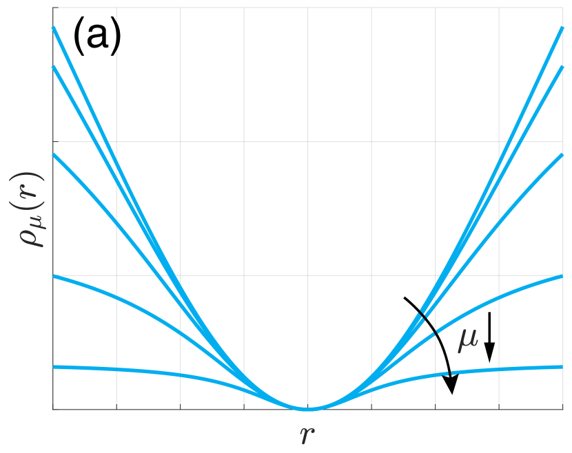
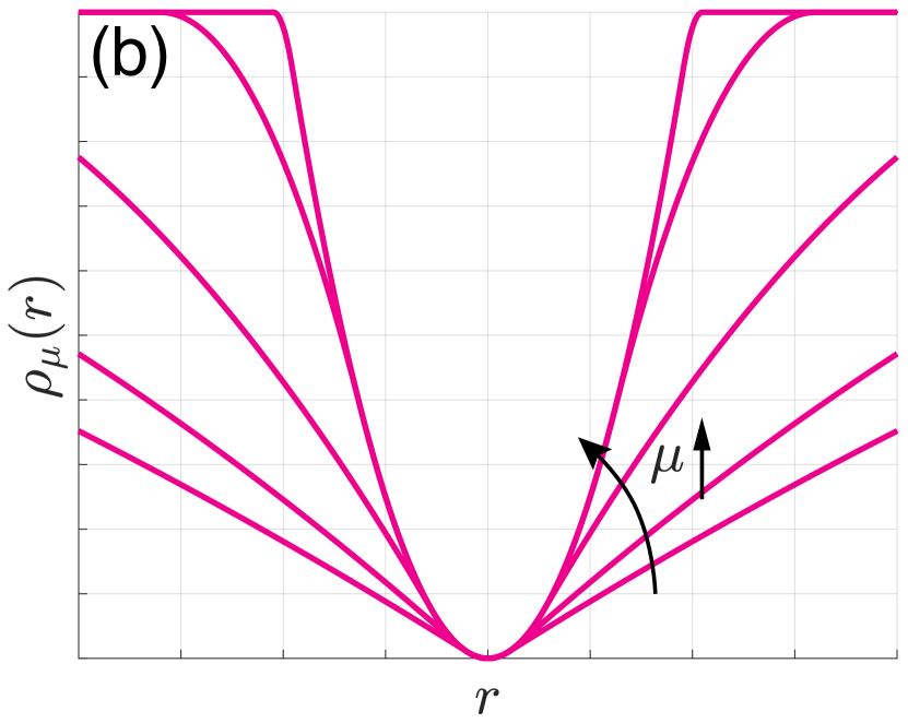
Graduated non-convexity (GNC) is a popular approach for the optimization of a generic non-convex cost function $\rho(\cdot)$ and has been used in several endeavors, including vision [33] and machine learning [45] (see [46] for more applications). The basic idea of GNC is to introduce a surrogate cost $\rho_{\mu}(\cdot)$, governed by a control parameter $\mu$, such that (i) for a certain value of $\mu$, the function $\rho_{\mu}(\cdot)$ is convex, and (ii) in the limit (typically for $\mu$ going to 1 or infinity) one recovers the original (non-convex) $\rho(\cdot)$. Then GNC computes a solution to the non-convex problem by starting from its convex surrogate and gradually changing $\mu$ (i.e., gradually increasing the amount of non-convexity) till the original non-convex function is recovered. The solution obtained at each iteration is used as the initial guess for the subsequent iteration.

Let us shed some light on GNC with two examples.

Example 1 (Geman McClure (GM) and GNC).

The Geman-McClure function is a popular (non-convex) robust cost. The following equation shows the GM function (left) and the surrogate function including a control parameter $\mu$ (right):

$$\rho(r)\doteq\frac{\bar{c}^{2}r^{2}}{\bar{c}^{2}+r^{2}}\;\;\Longrightarrow\;\;\rho_{\mu}(r)=\frac{\mu\bar{c}^{2}r^{2}}{\mu\bar{c}^{2}+r^{2}},$$ (4)

where $\bar{c}$ is a given parameter that determines the shape of the Geman McClure function $\rho(r)$.

The surrogate function $\rho_{\mu}(r)$ (shown in Fig. 1(a)) is such that: (i) $\rho_{\mu}(r)$ becomes convex for large $\mu$ (in the limit of $\mu\rightarrow\infty$, $\rho_{\mu}(r)$ becomes quadratic), and (ii) $\rho_{\mu}(r)$ recovers $\rho(r)$ when $\mu=1$. GNC minimizes the function $\rho(r)$ by repeatedly minimizing the function $\rho_{\mu}(r)$ for decreasing values of $\mu$.

Example 2 (Truncated Least Squares (TLS) and GNC).

The truncated least squares function is defined as:

$$\rho(r)=\begin{cases}\scriptstyle{r^{2}}&{\footnotesize\text{ if }}\scriptstyle{r^{2}\in\left[0,\bar{c}^{2}\right]}\\ \scriptstyle{\bar{c}^{2}}&{\footnotesize\text{ if }}\scriptstyle{r^{2}\in\left[\bar{c}^{2},+\infty\right)}\end{cases},$$ (5)

where $\bar{c}$ is a given truncation threshold. The GNC surrogate function with control parameter $\mu$ is:

$$\rho_{\mu}(r)=\begin{cases}\scriptstyle{r^{2}}&{\footnotesize\text{ if }}\scriptstyle{r^{2}\in\left[0,\frac{\mu}{\mu+1}\bar{c}^{2}\right]}\\ \scriptstyle{2\bar{c}|r|\sqrt{\mu(\mu+1)}-\mu(\bar{c}^{2}+r^{2})}&{\footnotesize\text{ if }}\scriptstyle{r^{2}\in\left[\frac{\mu}{\mu+1}\bar{c}^{2},\frac{\mu+1}{\mu}\bar{c}^{2}\right]}\\ \scriptstyle{\bar{c}^{2}}&{\footnotesize\text{ if }}\scriptstyle{r^{2}\in\left[\frac{\mu+1}{\mu}\bar{c}^{2},+\infty\right)}\end{cases}.$$ (6)

By inspection, one can verify $\rho_{\mu}(r)$ is convex for $\mu$ approaching zero ($\rho^{\prime\prime}_{\mu}(r)=-2\mu\rightarrow 0$) and retrieves $\rho(r)$ in (5) for $\mu\rightarrow+\infty$. An illustration of $\rho_{\mu}(r)$ is given in Fig. 1(b).

Figure 1: Graduated Non-Convexity (GNC) with control parameter $\mu$ for (a) Geman McClure (GM) and (b) Truncated Least Squares (TLS) costs.

IV The GNC Algorithm for Robust Estimation

We present an algorithm that combines GNC, Black-Rangarajan duality, and non-minimal solvers to solve the robust estimation problem (2) without an initial guess.

IV-A Overview: GNC Algorithm with Non-minimal Solvers

We start by providing an overview of the proposed algorithm, then we delve into technical details and tailor the approach to two specific robust cost functions (Section IV-B). Instead of optimizing directly the robust estimation problem (2), we use GNC and, at each outer iteration, we fix a $\mu$ and optimize:

$$\min_{{\bm{x}}\in{\cal X}}\sum_{i=1}^{N}\rho_{\mu}(r({\bm{y}}_{i},{\bm{x}})).$$ (7)

Since non-minimal solvers cannot be used directly to solve (7), we use the Black-Rangarajan duality and rewrite (7) using the corresponding outlier process:

$$\min_{{\bm{x}}\in{\cal X},w_{i}\in[0,1]}\sum_{i=1}^{N}\left[w_{i}r^{2}({\bm{y}}_{i},{\bm{x}})+\Phi_{\rho_{\mu}}(w_{i})\right].$$ (8)

As discussed in Section IV-B and [11], it is easy to compute the penalty terms $\Phi_{\rho_{\mu}}(\cdot)$ even for the surrogate function $\rho_{\mu}(\cdot)$.

Finally, we solve (8) by alternating optimization, where at each inner iteration we first optimize over the ${\bm{x}}$ (with fixed $w_{i}$), and then we optimize over $w_{i}$, $i=1,\ldots,N$ (with fixed ${\bm{x}}$). In particular, at inner iteration $t$, we perform the following:

1. Variable update: minimize (8) with respect to ${\bm{x}}$ with fixed weights $w^{(t-1)}_{i}$:

   $${\bm{x}}^{(t)}=\operatorname*{arg\,min}_{{\bm{x}}\in{\cal X}}\sum_{i=1}^{N}w^{(t-1)}_{i}r^{2}({\bm{y}}_{i},{\bm{x}}),$$ (9)

   where we dropped the second term in (8) which does not depend on ${\bm{x}}$. Problem (9) is simply a weighted version of the outlier-free problem (1), hence it can be solved globally using certifiably optimal non-minimal solvers.

2. Weight update: minimize (8) with respect to $w_{i}$ ($i=1,\ldots,N$) with fixed ${\bm{x}}^{(t)}$:

   $${\bm{w}}^{(t)}=\operatorname*{arg\,min}_{w_{i}\in[0,1]}\sum_{i=1}^{N}\left[w_{i}r^{2}({\bm{y}}_{i},{\bm{x}}^{(t)})+\Phi_{\rho_{\mu}}(w_{i})\right],$$ (10)

   where $r^{2}({\bm{y}}_{i},{\bm{x}}^{(t)})$ is a constant for fixed ${\bm{x}}$, and the expression of $\Phi_{\rho_{\mu}}(\cdot)$ depends on the choice of robust cost function. As we discuss in Section IV-B, the weight update can be typically solved in closed form.

The process is then repeated for changing values of $\mu$, where each change of $\mu$ increases the amount of non-convexity.

Remark 2 (Teaching an Old Dog New Tricks).

While the combination of GNC and Black-Rangarajan duality has been investigated in related works [11, 35], its applicability has been limited by the lack of global solvers for the variable update in (9). For instance, [35] focuses on a specific problem (point cloud registration) where (9) can be solved in closed form [36, 3], while [11] focuses on a Markov Random Field formulation for which global solvers and heuristics exist [47]. One of the main insights behind our approach is that modern non-minimal solvers (developed over the last 5 years) allow solving (9) globally for a broader class of problems, including spatial perception problems such as SLAM, mesh registration, and object localization from images.

Figure 2: Point Cloud Registration. Performance of GNC-GM and GNC-TLS compared with state-of-the-art techniques on the Bunny dataset [48] for increasing outliers. (a) rotation error; (b) translation error; (c) number of iterations until convergence. Statistics are computed over 20 Monte Carlo runs.

Figure 3: Mesh Registration. Performance of GNC-GM and GNC-TLS compared with state-of-the-art techniques on mesh registration on the PASCAL+ “car-2” dataset [49] for increasing outliers. Quantitative results: (a) rotation error; (b) translation error; (c) number of iterations until convergence. Qualitative results: (d) point cloud and mesh with putative correspondences (70% outliers; green: inliers, red: outliers); (e) successful registration using GNC-TLS; (f) incorrect registration using RANSAC. Statistics are computed over 20 Monte Carlo runs.

IV-B The GNC Algorithm with GM and TLS Costs

Here we tailor the GNC algorithm to two cost functions, the Geman McClure and the Truncated Least Squares costs, provide expressions for the penalty term $\Phi_{\rho_{\mu}}$, and discuss how to solve the weight update step. The proofs of the following propositions are given in the supplementary material [50].

Proposition 3 (GNC-Geman McClure (GNC-GM)).

Consider the Geman-McClure function and its GNC surrogate with control parameter $\mu$, as introduced in Example 1. Then, the minimization of the surrogate function $\rho_{\mu}(\cdot)$ is equivalent to the outlier process with penalty term chosen as:

$$\Phi_{\rho_{\mu}}(w_{i})=\mu\bar{c}^{2}(\sqrt{w_{i}}-1)^{2}.$$ (11)

Moreover, defining the residual $\hat{r}_{i}^{2}\doteq r^{2}({\bm{y}}_{i},{\bm{x}}^{(t)})$, the weight update at iteration $t$ can be solved in closed form as:

$$w_{i}^{(t)}=\left(\frac{\mu\bar{c}^{2}}{\hat{r}_{i}^{2}+\mu\bar{c}^{2}}\right)^{2}\!.$$ (12)

Proposition 4 (GNC-Truncated Least Squares (GNC-TLS)).

Consider the truncated least squares function and its GNC surrogate with control parameter $\mu$, as introduced in Example 2. Then, the minimization of the surrogate function $\rho_{\mu}(\cdot)$ is equivalent to the outlier process with penalty term:

$$\Phi_{\rho_{\mu}}(w_{i})=\frac{\mu(1-w_{i})}{\mu+w_{i}}\bar{c}^{2}.$$ (13)

Moreover, defining the residual $\hat{r}_{i}^{2}\doteq r^{2}({\bm{y}}_{i},{\bm{x}}^{(t)})$, the weight update at iteration $t$ can be solved in closed form as:

$$w_{i}^{(t)}=\begin{cases}0&\text{ if }\hat{r}_{i}^{2}\in\left[\frac{\mu+1}{\mu}\bar{c}^{2},+\infty\right]\\ \frac{\bar{c}}{\hat{r}_{i}}\sqrt{\mu(\mu+1)}-\mu&\text{ if }\hat{r}_{i}^{2}\in\left[\frac{\mu}{\mu+1}\bar{c}^{2},\frac{\mu+1}{\mu}\bar{c}^{2}\right]\\ 1&\text{ if }\hat{r}_{i}^{2}\in\left[0,\frac{\mu}{\mu+1}\bar{c}^{2}\right].\end{cases}$$ (14)

Remark 5 (Implementation Details).

For GNC-GM, we start with a convex surrogate ($\mu\kern-5.0pt\rightarrow\kern-5.0pt\infty$) and decrease $\mu$ till we recover the original cost ($\mu\!\rightarrow\!1$). In practice, calling $r_{\max}^{2}\doteq\max_{i}(r^{2}({\bm{y}}_{i},{\bm{x}}^{(0)}))$ the maximum residual after the first variable update, we initialize $\mu\!=\!2r^{2}_{\max}/\bar{c}^{2}$, update $\mu\leftarrow\mu/1.4$ at each outer iteration, and stop when $\mu$ decreases below $1$. For GNC-TLS, we start with a convex surrogate ($\mu\rightarrow 0$) and increase the $\mu$ till we recover the original cost ($\mu\kern-1.99997pt\rightarrow\kern-1.99997pt\infty$). In practice, we initialize $\mu\!=\!\bar{c}^{2}/(2r^{2}_{\max}-\bar{c}^{2})$, update $\mu\!\leftarrow\!1.4\mu$ at each outer iteration, and stop when the sum of the weighted residuals $\sum_{i=1}^{N}w_{i}\hat{r}_{i}^{2}$ converges. For each outer iteration we perform a single variable and weight update. At the first iteration, all weights are set to 1 ($w_{i}^{(0)}=1,i=1,\dots,N$). For both robust functions, we set the parameter $\bar{c}$ to the maximum error expected for the inliers, see Remarks 1-2 in [14].

V Applications and Experiments

We showcase our robust non-minimal solvers in three spatial perception applications: point cloud and mesh registration (Section V-A), pose graph optimization (Section V-B), and shape alignment (Section V-C).

V-A 3D Point Cloud and Mesh Registration

Setup. In generalized 3D registration, given a set of 3D points ${\bm{a}}_{i}\in{{\mathbb{R}}^{3}}$, $i=1,\ldots,N$, and a set of primitives ${\bm{P}}_{i}$, $i=1,\ldots,N$ (being points, lines and/or planes) with putative correspondences ${\bm{a}}_{i}\leftrightarrow{\bm{P}}_{i}$ (potentially including outliers), the goal is to find the best rotation ${\bm{R}}\in\mathrm{SO}(3)$ and translation ${\bm{t}}\in{{\mathbb{R}}^{3}}$ that align the point cloud to the 3D primitives. The residual error is $r({\bm{R}},{\bm{t}})=d({\bm{P}}_{i},{\bm{R}}{\bm{a}}_{i}+{\bm{t}})$, where $d(\cdot)$ denotes the distance between a primitive ${\bm{P}}_{i}$ and a point ${\bm{a}}_{i}$ after the transformation $({\bm{t}},{\bm{R}})$ is applied. The formulation can also accommodate weighted distances to account for heterogeneous and anisotropic measurement noise. In the outlier-free case, Horn’s method [3] gives a closed-form solution when all the 3D primitives are points and the noise is isotropic, and [8] develops a certifiably optimal relaxation when the 3D primitives include points, lines, and planes and the noise is anisotropic. We now show that, using the GNC-GM and GNC-TLS solvers, we can efficiently robustify these non-minimal solvers. We benchmark our algorithms against state-of-the-art techniques in point cloud registration and mesh registration.

Figure 4: Pose Graph Optimization. Performance of GNC-GM and GNC-TLS compared with state-of-the-art techniques for increasing outliers. Average trajectory error for (a) INTEL dataset and (b) CSAIL dataset; (c) solution time on the CSAIL dataset. Statistics are computed over 10 Monte Carlo runs.

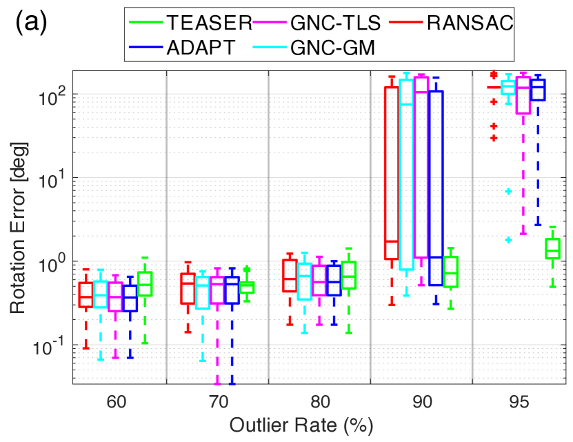
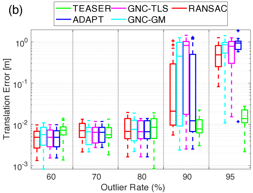
Point Cloud Registration Results. We use the Bunny dataset from the Stanford 3D Scanning Repository [48]. We first scale the Bunny point cloud to be inside a unit cube, and then at each Monte Carlo run we apply a random rotation and translation to get a transformed copy of the Bunny. $N=100$ correspondences are randomly chosen, where we add zero-mean Gaussian noise with standard deviation $\sigma=0.01$ to the inliers, while corrupt the outliers with randomly generated points as in [2]. We benchmark the performance of GNC-GM and GNC-TLS against (i) RANSAC with 1000 maximum iterations and $99\%$ confidence using Horn’s 3-point minimal solver [3], plus refinement using the maximum consensus set of inliers, (ii) ADAPT [27], and (iii) TEASER [2].

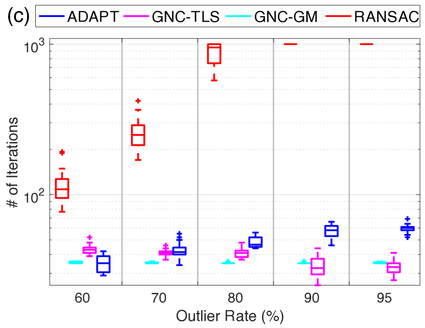
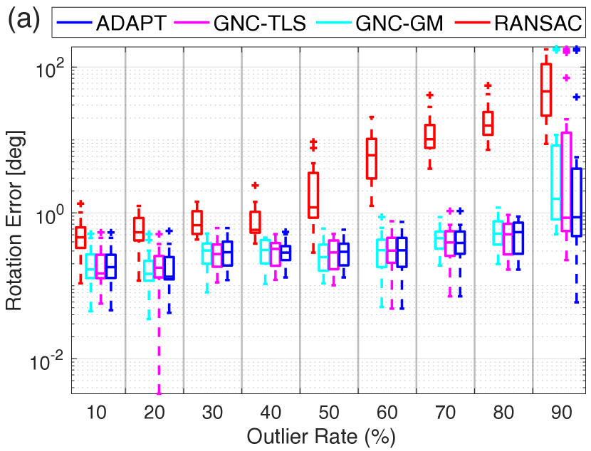
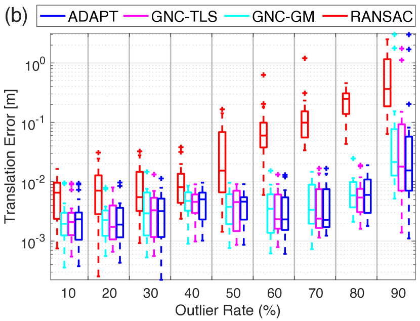
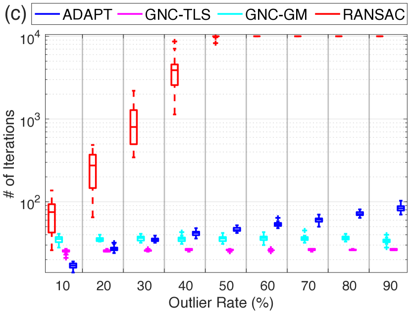
Fig. 2 reports the statistics for $60\%$-$95\%$ outlier rates (all methods work well below $60\%$). Fig. 2(a)-(b) show the rotation and translation errors for increasing outliers. RANSAC, GNC-GM, GNC-TLS, and ADAPT all break at 90% outliers and achieve similar estimation accuracy at outlier ratio below 90%. TEASER is a specialized robust global solver and outperforms all other techniques; unfortunately, it currently does not scale to large problem instances (>5min runtime) and does not extend to other registration problems (e.g., mesh registration); Fig. 2(c) plots the number of inner iterations used by RANSAC, GNC-GM, GNC-TLS, and ADAPT (TEASER has no outlier iterations). With respect to the outlier rates, the number of iterations grows very fast for RANSAC, grows linearly for ADAPT and is almost constant for GNC-GM and GNC-TLS. At $80\%$ outliers, the average runtimes for RANSAC, GNC-GM, and GNC-TLS are $218$, $22$ and $23$ms, respectively, showing that GNC can be much faster than RANSAC. For point cloud registration, GNC-GM is essentially the same as Fast Global Registration [35], while below we show that the use of non-minimal solvers allows extending GNC to other spatial perception applications.

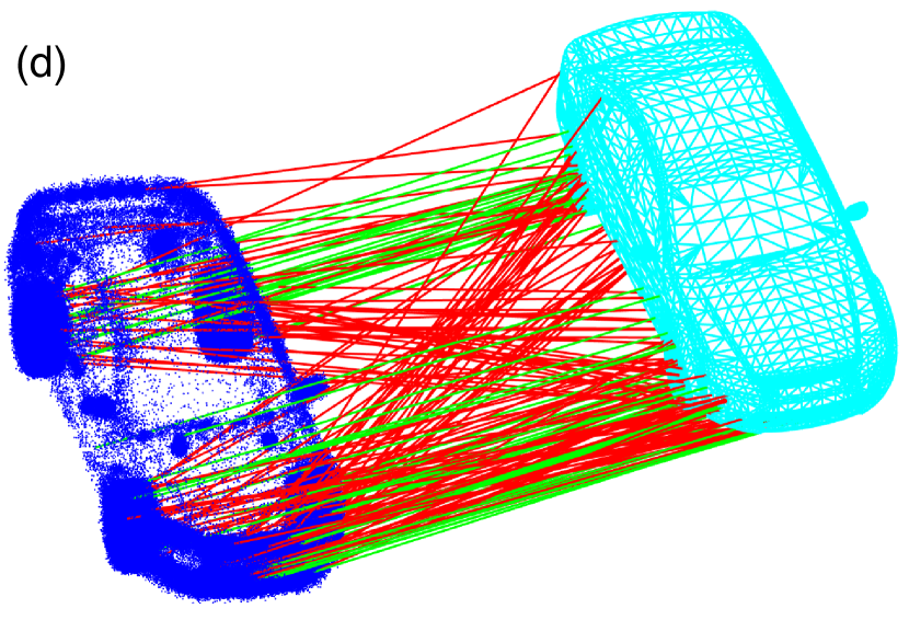
Mesh Registration Results. We apply GNC-GM and GNC-TLS to register a point cloud to a mesh, using the non-minimal solver [8]. We use the “car-2” mesh model from the PASCAL+ dataset [49]. At each Monte Carlo run, we generate a point cloud from the mesh by randomly sampling points lying on the vertices, edges and faces of the mesh model, and then apply a random transformation and add Gaussian noise with $\sigma=0.05$. We establish 40 point-to-point, 80 point-to-line and 80 point-to-plane correspondences, and create outliers by adding incorrect point to point/line/plane correspondences (Fig. 3(d)). We benchmark GNC-GM and GNC-TLS against (i) RANSAC with 10,000 maximum iterations and $99\%$ confidence using the 12-point minimal solver in [17] and (ii) ADAPT [27].

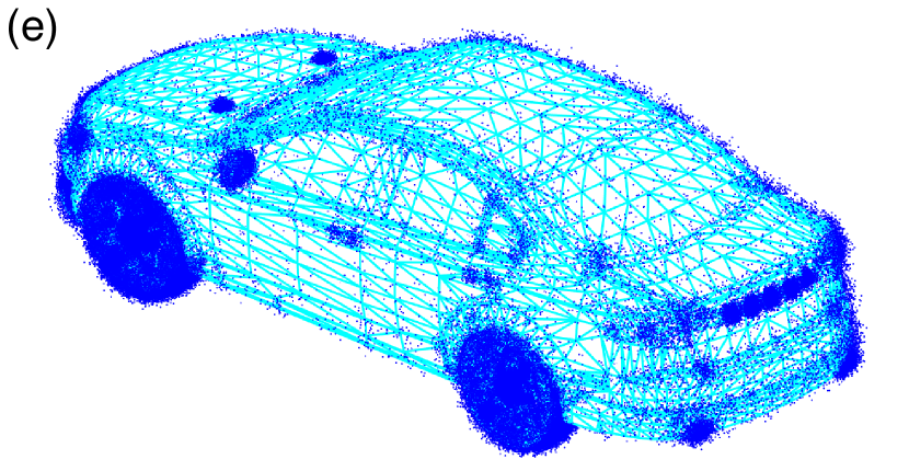
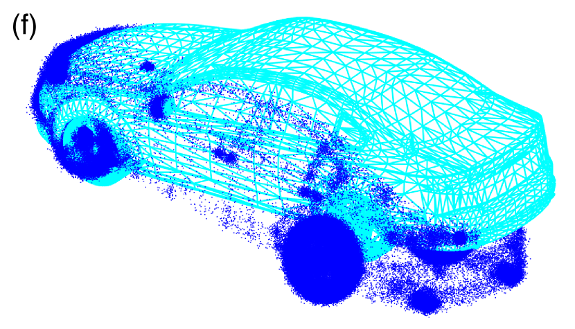
Fig. 3(a)-(c) show the errors and iterations for each technique. GNC-GM, GNC-TLS, and ADAPT are robust against 80% outliers, while RANSAC breaks at 50% outliers. The number of iterations of ADAPT grows linearly with the number of outliers, while GNC-GM’s and GNC-TLS’s iterations remain constant. Fig. 3(e) shows a successful registration with GNC-TLS and Fig. 3(f) shows an incorrect registration from RANSAC, both obtained in a test with 70% outliers.

V-B Pose Graph Optimization

Setup. PGO is one of the most common estimation engines for SLAM [1]. PGO estimates a set of poses $({\bm{t}}_{i},{\bm{R}}_{i})$, $i=1,\ldots,n$ (typically sampled along the robot trajectory) from pairwise relative pose measurements $(\tilde{{\bm{t}}}_{ij},\tilde{{\bm{R}}}_{ij})$ (potentially corrupted with outliers). The residual error is the distance between the expected relative pose and the measured one:

$$r(\{{\bm{R}}_{i},{\bm{t}}_{i}\})\!=\!\sqrt{\kappa_{ij}\|{\bm{R}}_{j}-{\bm{R}}_{i}\tilde{{\bm{R}}}_{ij}\|_{F}^{2}+\tau_{ij}\|{\bm{t}}_{j}-{\bm{t}}_{i}-{\bm{R}}_{i}\tilde{{\bm{t}}}_{ij}\|^{2}_{2}},$$

where $\kappa_{ij}$ and $\tau_{ij}$ are known parameters describing the measurement noise distribution, and $\|\cdot\|_{F}$ denotes the Frobenious norm. SE-Sync [6] is a fast non-minimal solver for PGO.

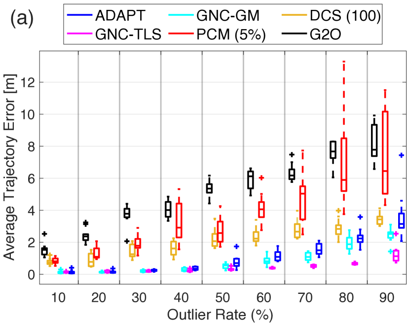
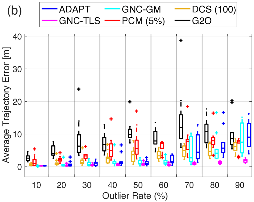
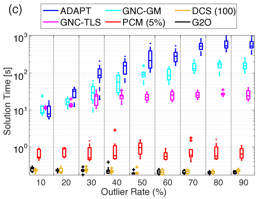
PGO Results. We test GNC-GM and GNC-TLS on two standard benchmarking datasets: INTEL and CSAIL, described in [6]. In each dataset, we preserve the odometry measurements, but at each Monte Carlo run we spoil loop closures with random outliers. To create outliers, we sample random pairs of poses and add a random measurement between them. We benchmark GNC-GM and GNC-TLS against (i) g2o [20], (ii) dynamic covariance scaling (DCS) [42], (iii) pairwise consistent measurement set maximization (PCM) [30], and (iv) ADAPT [27]. DCS and PCM are fairly sensitive to the choice of parameters: we tested parameters $\Phi=\{1,10,100\}$ for DCS, and thresholds $\tau=\{5\%,10\%,15\%\}$ for PCM, and, for the sake of clarity, we only reported the choice of parameters ensuring the best performance.

Fig. 4(a) shows the average trajectory errors for the INTEL dataset. g2o is not a robust solver and performs poorly across the spectrum. DCS and PCM are specialized robust local solvers, but their errors gradually increase with the percentage of outliers. GNC-GM, GNC-TLS, and ADAPT are insensitive to up to $40\%$ outliers and preserve an acceptable performance till $70-80\%$ of outliers; GNC-TLS dominates the others. Fig. 4(b) reports the results on the CSAIL dataset. Also in this case, GNC-TLS dominates the other techniques and is robust to 90% outliers. Fig. 4(c) reports the CPU times required by the techniques to produce a solution on CSAIL; in this case, all techniques are implemented in C++.

Figure 5: Shape Alignment. Performance of GNC-GM and GNC-TLS compared with state-of-the-art techniques on the FG3DCar dataset [51] for increasing outliers. Quantitative results: (a) rotation error; (b) translation error; (c) number of iterations. Qualitative results with 70% outliers: (d) successful pose estimation by GNC-GM; (e) failed pose estimation by RANSAC; (f) failed pose estimation by Zhou’s method [15]. Yellow thick line: 3D skeleton of the car model; circle: 3D points on the car model; square: detected 2D features on the image; green: inlier correspondences; red: outlier correspondences.

V-C Shape Alignment

Setup. In shape alignment, given 2D features ${\bm{z}}_{i}\in{{\mathbb{R}}^{2}},i=1,\ldots,N$, on a single image and 3D points ${\bm{B}}_{i}\in{{\mathbb{R}}^{3}},i=1,\ldots,N$, of an object with putative correspondences ${\bm{z}}_{i}\leftrightarrow{\bm{B}}_{i}$ (potentially including outliers), the goal is to find the best scale $s>0$, rotation ${\bm{R}}$, and translation ${\bm{t}}$ of the object, that projects the 3D shape to the 2D image under weak perspective projection. The residual function is $r(s,{\bm{R}},{\bm{t}})=\|{\bm{z}}_{i}-s\Pi{\bm{R}}{\bm{B}}_{i}-{\bm{t}}\|$, where $\Pi\in{{\mathbb{R}}^{2\times 3}}$ is the weak perspective projection matrix (equal to the first two rows of a $3\!\times\!3$ identity matrix). Note that ${\bm{t}}$ is a 2D translation, but under weak perspective projection one can extrapolate a 3D translation (i.e., recover the distance of the camera to the object) using the scale $s$.

A Non-minimal Solver for Shape Alignment. The literature is missing a global solver for shape alignment, even in the outlier-free case. Therefore, we start by proposing a non-minimal solver for (weighted) outlier-free shape alignment:

$$\min_{s>0,{\bm{R}}\in\mathrm{SO}(3),{\bm{t}}\in{{\mathbb{R}}^{2}}}\textstyle{\sum_{i=1}^{N}}w_{i}\|{\bm{z}}_{i}-s\Pi{\bm{R}}{\bm{B}}_{i}-{\bm{t}}\|^{2},$$ (15)

where $w_{i}$ are constant weights. The next proposition states that the global minimizer of problem (15) can be obtained by solving a quaternion-based unconstrained optimization.

Proposition 6 (Quaternion-based Shape Alignment).

Define the non-unit quaternion ${\bm{v}}\doteq\sqrt{s}{\bm{q}}\in{{\mathbb{R}}^{4}}$, where ${\bm{q}}$ is the unit-quaternion corresponding to ${\bm{R}}$ and $s$ is the unknown scale. Moreover, if ${\bm{v}}=[v_{1},v_{2},v_{3},v_{4}]^{\mathsf{T}}$, define $[{\bm{v}}]_{2}\doteq[v_{1}^{2},v_{2}^{2},v_{3}^{2},v_{4}^{2},v_{1}v_{2},v_{1}v_{3},v_{1}v_{4},v_{2}v_{3},v_{2}v_{4},v_{3}v_{4}]^{\mathsf{T}}\in{{\mathbb{R}}^{10}}$ as the vector of degree-2 monomials in ${\bm{v}}$. Then the globally optimal solutions ($s^{\star},{\bm{R}}^{\star},{\bm{t}}^{\star}$) of problem (15) can be obtained from the solution ${\bm{v}}^{\star}$ of the following optimization:

$$\min_{{\bm{v}}\in{{\mathbb{R}}^{4}}}f({\bm{v}})\doteq[{\bm{v}}]_{2}^{\mathsf{T}}{\bm{Q}}[{\bm{v}}]_{2}-2{\bm{g}}^{\mathsf{T}}[{\bm{v}}]_{2}+h,$$ (16)

where ${\bm{Q}}\in{{\mathbb{R}}^{10\times 10}}$, ${\bm{g}}\in{{\mathbb{R}}^{10}}$, and $h>0$ are known quantities, whose expression is given in the supplementary material [50].

Problem (16) requires minimizing a degree-4 polynomial $f({\bm{v}})$ in 4 variables; to this end, we apply SOS relaxation and relax (16) to the following SOS optimization:

$$\min_{{\bm{v}}\in{{\mathbb{R}}^{4}},\gamma\in{{\mathbb{R}}}} -\gamma\quad,\quad\text{s.t.}\quad f({\bm{v}})-\gamma\text{ is SOS},$$ (17)

which can be readily converted to an SDP and solved with certifiable optimality [4]. We use the GloptiPoly 3 [52] package in Matlab to solve problem (17) and found that empirically the relaxation is always exact. Solving the SDP takes about 80 ms on a desktop computer.

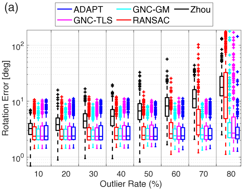
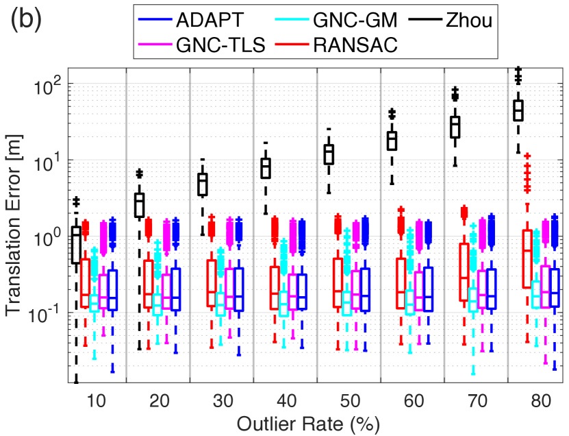
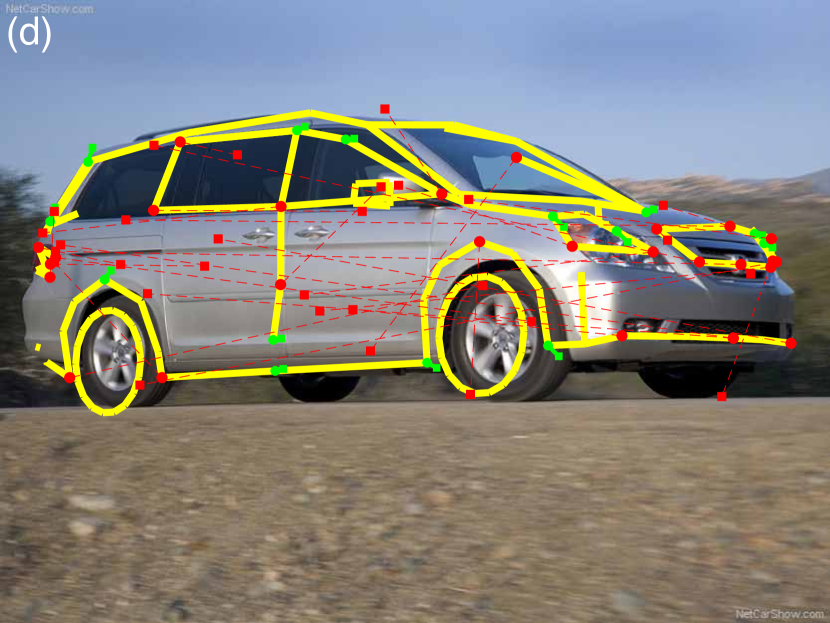
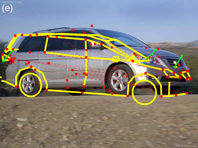
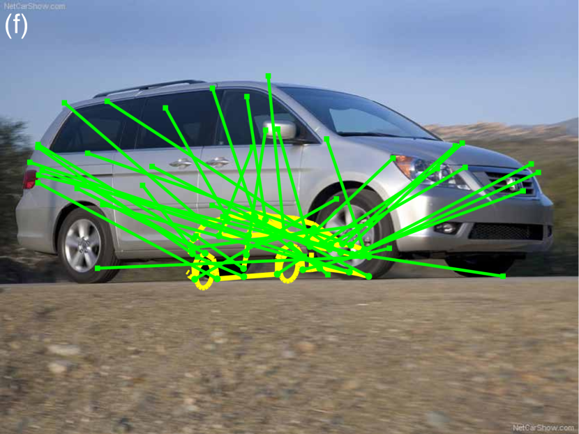
Shape Alignment Results. We test the performance of GNC-GM and GNC-TLS, together with our SOS solver on the FG3DCar dataset [51], where we use the ground-truth 3D shape model as ${\bm{B}}$ and the ground-truth 2D landmarks as ${\bm{z}}$. To generate outliers for each image, we set random incorrect correspondences between 3D points and 2D features. We benchmark GNC-GM and GNC-TLS against (i) Zhou’s method [15], (ii) RANSAC with 100 maximum iterations and $99\%$ confidence using a 4-point minimal solver (we use our SOS solver as minimal solver), and (iii) ADAPT [27].

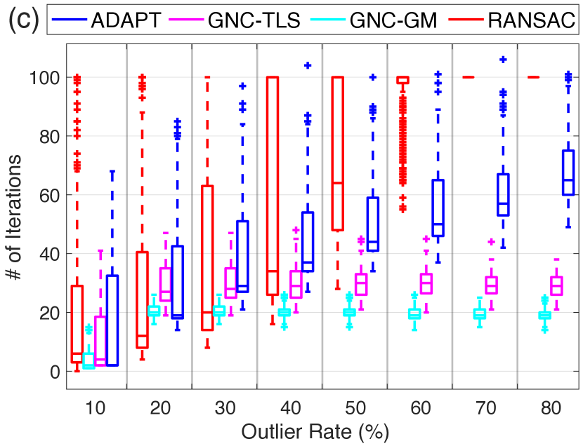
Fig 5(a)-(c) show translation errors, rotation errors, and number of iterations for all compared techniques. Statistics are computed over all 600 images in the FG3DCar dataset. The performance of Zhou’s method degrades quickly with increasing outliers. RANSAC breaks at 60% outliers. GNC-GM, GNC-TLS, and ADAPT are robust against 70% outliers, while GNC-GM and GNC-TLS require a roughly constant number of iterations. Qualitative results for GNC-GM, RANSAC, and Zhou’s approach are given in Fig. 5(d)-(f), respectively.

VI Conclusions

We proposed a general-purpose approach for robust estimation that leverages modern non-minimal solvers. The approach allows extending the applicability of Black-Rangarajan duality and Graduated Non-convexity (GNC) to several spatial perception problems, ranging from mesh registration and shape alignment to pose graph optimization. We believe the proposed approach can be a valid replacement for RANSAC. While RANSAC requires a minimal solver, our GNC approach requires a non-minimal solver. Our approach is deterministic, resilient to a large number of outliers, and significantly faster than specialized solvers. As a further contribution, we presented a non-minimal solver for shape alignment. Future work includes investigating a priori and a posterior conditions that guarantee convergence of GNC to globally optimal solutions.

Supplementary Material

VII Proof of Proposition 3

The outlier process (11) is derived by following the Black-Rangarajan procedure in Fig. 10 of [11]. Therefore, we here prove the weight update rule in eq. (12). To this end, we derive the gradient $g_{i}$ of the objective function with outlier process $\Phi_{\rho_{\mu}}(w_{i})=\mu\bar{c}^{2}(\sqrt{w_{i}}-1)^{2}$ in eq. (10) with respect to $w_{i}$:

$$g_{i}=\hat{r}_{i}^{2}+\mu\bar{c}^{2}\left(1-\frac{1}{\sqrt{w_{i}}}\right).$$ (A18)

From eq. (A18) we observe that if $w_{i}\rightarrow 0$, then $g_{i}\rightarrow-\infty$; and if $w_{i}=1$, then $g_{i}=\hat{r}_{i}^{2}\geq 0$. These facts, combined with the monotonicity of $g_{i}$ w.r.t. $w_{i}$, ensure that there exists a unique $w_{i}^{\star}$ such that the gradient $g_{i}$ vanishes:

$$w_{i}^{\star}=\left(\frac{\mu\bar{c}^{2}}{\hat{r}_{i}^{2}+\mu\bar{c}^{2}}\right)^{2}.$$ (A19)

This vanishing point is the global minimizer of (10).

VIII Proof of Proposition 4

The outlier process (13) is derived by following the Black-Rangarajan procedure in Fig. 10 of [11]. Therefore, we here prove the weight update rule in eq. (14). To this end, we derive the gradient $g_{i}$ of the objective function with outlier process $\Phi_{\rho_{\mu}}(w_{i})=\frac{\mu(1-w_{i})}{\mu+w_{i}}$ in eq. (10) with respect to $w_{i}$:

$$g_{i}=\hat{r}_{i}^{2}-\frac{\mu(\mu+1)}{(\mu+w_{i})^{2}}\bar{c}^{2}.$$ (A20)

From eq. (A20) we observe that if $w_{i}=0$, then $g_{i}=\hat{r}_{i}^{2}-\frac{\mu+1}{\mu}\bar{c}^{2}$; and if $w_{i}=1$, then $g_{i}=\hat{r}_{i}^{2}-\frac{\mu}{\mu+1}\bar{c}^{2}$. Therefore, the global minimizer $w_{i}^{\star}$ can be obtained by setting the gradient $g_{i}$ to zero, leading to:

$$w_{i}^{\star}=\begin{cases}0&\text{ if }\hat{r}_{i}^{2}\in\left[\frac{\mu+1}{\mu}\bar{c}^{2},+\infty\right]\\ \frac{\bar{c}}{\hat{r}_{i}}\sqrt{\mu(\mu+1)}-\mu&\text{ if }\hat{r}_{i}^{2}\in\left[\frac{\mu}{\mu+1}\bar{c}^{2},\frac{\mu+1}{\mu}\bar{c}^{2}\right]\\ 1&\text{ if }\hat{r}_{i}^{2}\in\left[0,\frac{\mu}{\mu+1}\bar{c}^{2}\right]\end{cases}.$$ (A21)

IX Proof of Proposition 6

In the main document, we claim that the optimal solutions $(s^{\star},{\bm{R}}^{\star},{\bm{t}}^{\star})$ for the shape alignment problem

$$\min_{s>0,{\bm{R}}\in\mathrm{SO}(3),{\bm{t}}\in{{\mathbb{R}}^{2}}}\textstyle{\sum_{i=1}^{N}}w_{i}\|{\bm{z}}_{i}-s\Pi{\bm{R}}{\bm{B}}_{i}-{\bm{t}}\|^{2}$$ (A22)

can be obtained from the optimal solution ${\bm{v}}^{\star}$ of the quaternion-based unconstrained optimization:

$$\min_{{\bm{v}}\in{{\mathbb{R}}^{4}}}f({\bm{v}})\doteq[{\bm{v}}]_{2}^{\mathsf{T}}{\bm{Q}}[{\bm{v}}]_{2}-2{\bm{g}}^{\mathsf{T}}[{\bm{v}}]_{2}+h.$$ (A23)

Here we prove this proposition, and provide a formula to compute ${\bm{Q}}\in{{\mathbb{R}}^{10\times 10}}$, ${\bm{g}}\in{{\mathbb{R}}^{10}}$ and $h$, as well as construct $(s^{\star},{\bm{R}}^{\star},{\bm{t}}^{\star})$ from ${\bm{v}}^{\star}$. Particularly, we complete the proof in two steps: (i) we marginalize out the translation ${\bm{t}}$ and convert problem (A22) into an equivalent translation-free problem; (ii) we reparametrize the rotation matrix using unit-quaternion and then arrive at the unconstrained optimization in (A23). The two steps follow in more detail below:

(i) Translation-free Shape Alignment. To this end, we develop the objective function of (A22):

$$\sum_{i=1}^{N}w_{i}\|{\bm{z}}_{i}-s\Pi{\bm{R}}{\bm{B}}_{i}-{\bm{t}}\|^{2}$$

$$=\sum_{i=1}^{N}w_{i}{\bm{t}}^{\mathsf{T}}{\bm{t}}-2w_{i}({\bm{z}}_{i}^{\mathsf{T}}-s{\bm{B}}_{i}^{\mathsf{T}}{\bm{R}}^{\mathsf{T}}\Pi^{\mathsf{T}}){\bm{t}}$$

$$+\sum_{i=1}^{N}\|{\bm{z}}_{i}-s\Pi{\bm{R}}{\bm{B}}_{i}\|^{2},$$ (A24)

whose partial derivative w.r.t. ${\bm{t}}$ is:

$$2\sum_{i=1}^{N}w_{i}{\bm{t}}-2\left(\sum_{i=1}^{N}w_{i}{\bm{z}}_{i}-s\Pi{\bm{R}}\sum_{i=1}^{N}w_{i}{\bm{B}}_{i}\right).$$ (A25)

By setting the derivative (A25) to zero, we derive ${\bm{t}}^{\star}$ in closed form as:

$${\bm{t}}^{\star}=\bar{{\bm{z}}}_{w}-s^{\star}\Pi{\bm{R}}^{\star}\bar{{\bm{B}}}_{w},$$ (A26)

where

$$\bar{{\bm{z}}}_{w}=\frac{\sum_{i=1}^{N}w_{i}{\bm{z}}_{i}}{\sum_{i=1}^{N}w_{i}},\quad\bar{{\bm{B}}}_{w}=\frac{\sum_{i=1}^{N}w_{i}{\bm{B}}_{i}}{\sum_{i=1}^{N}w_{i}}.$$ (A27)

By inserting eq. (A26) back to the original problem (A22), we obtain an optimization only involving the scale and rotation:

$$\min_{s>0,{\bm{R}}\in\mathrm{SO}(3)}\sum_{i=1}^{N}\|\tilde{{\bm{z}}}_{i}-s\Pi{\bm{R}}\tilde{{\bm{B}}}_{i}\|^{2},$$ (A28)

where:

$$\tilde{{\bm{z}}}_{i}=\sqrt{w_{i}}({\bm{z}}_{i}-\bar{{\bm{z}}}_{w}),\quad\tilde{{\bm{B}}}_{i}=\sqrt{w_{i}}({\bm{B}}_{i}-\bar{{\bm{B}}}_{w}).$$ (A29)

(ii) Quaternion-based Translation-free Problem. We now show that the translation-free shape alignment problem (A28) can be converted to the quaternion-based unconstrained shape alignment problem (A23). To this end, we denote ${\bm{q}}\in{{\mathbb{R}}^{4}},\|{\bm{q}}\|=1$ as the unit-quaternion corresponding to the rotation matrix ${\bm{R}}$. It can be verified by inspection that ${\bm{R}}$ is a linear function of $[{\bm{q}}]_{2}\in{{\mathbb{R}}^{10}}$, the vector of all degree-2 monomials of ${\bm{q}}$:

$${\bm{R}}={\cal R}({\bm{q}})\doteq\text{mat}({\bm{A}}[{\bm{q}}]_{2}),$$ (A30)

where ${\bm{A}}\in{{\mathbb{R}}^{9\times 10}}$ is a constant matrix, and $\text{mat}(\cdot)$ converts a vector to a matrix with proper dimension (in this case a $3\times 3$ matrix). The expression of the matrix ${\bm{A}}$ is as follows:

$${\bm{A}}=\left[\begin{array}[]{cccccccccc}1&-1&-1&1&0&0&0&0&0&0\\ 0&0&0&0&2&0&0&0&0&2\\ 0&0&0&0&0&2&0&0&-2&0\\ 0&0&0&0&2&0&0&0&0&-2\\ -1&1&-1&1&0&0&0&0&0&0\\ 0&0&0&0&0&0&2&2&0&0\\ 0&0&0&0&0&2&0&0&2&0\\ 0&0&0&0&0&0&-2&2&0&0\\ -1&-1&1&1&0&0&0&0&0&0\end{array}\right].$$ (A40)

Using the notation in (A30) and developing the squares in the objective function of problem (A28) (denoting ${\bm{r}}=\mathrm{vec}\left({\bm{R}}\right)$):

$$\displaystyle\sum_{i=1}^{N}\|\tilde{{\bm{z}}}_{i}-s\Pi{\bm{R}}\tilde{{\bm{B}}}_{i}\|^{2}$$ (A41)

$$=\displaystyle\sum_{i=1}^{N}\|\tilde{{\bm{z}}}_{i}\|^{2}-2s\;\tilde{{\bm{z}}}_{i}^{\mathsf{T}}\Pi{\bm{R}}\tilde{{\bm{B}}}_{i}+s^{2}\tilde{{\bm{B}}}_{i}^{\mathsf{T}}{\bm{R}}^{\mathsf{T}}\Pi^{\mathsf{T}}\Pi{\bm{R}}\tilde{{\bm{B}}}_{i}$$

$$=\displaystyle\sum_{i=1}^{N}\|\tilde{{\bm{z}}}_{i}\|^{2}-2s\;\mathrm{tr}\left(\tilde{{\bm{B}}}_{i}{\bm{z}}_{i}^{\mathsf{T}}\Pi{\bm{R}}\right)+s^{2}\mathrm{tr}\left(\tilde{{\bm{B}}}_{i}\tilde{{\bm{B}}}_{i}^{\mathsf{T}}{\bm{R}}^{\mathsf{T}}\Pi^{\mathsf{T}}\Pi{\bm{R}}\right)$$

$$=\displaystyle\sum_{i=1}^{N}\|\tilde{{\bm{z}}}_{i}\|^{2}-2s\;\mathrm{vec}\left(\Pi^{\mathsf{T}}\tilde{{\bm{z}}}_{i}\tilde{{\bm{B}}}_{i}^{\mathsf{T}}\right)^{\mathsf{T}}{\bm{r}}+s^{2}{\bm{r}}^{\mathsf{T}}(\tilde{{\bm{B}}}_{i}\tilde{{\bm{B}}}_{i}^{\mathsf{T}}\otimes\Pi^{\mathsf{T}}\Pi){\bm{r}}$$

$$=\displaystyle\sum_{i=1}^{N}\|\tilde{{\bm{z}}}_{i}\|^{2}-2s\;{\bm{f}}_{i}^{\mathsf{T}}{\bm{A}}[{\bm{q}}]_{2}+s^{2}[{\bm{q}}]_{2}^{\mathsf{T}}{\bm{A}}^{\mathsf{T}}{\bm{F}}_{i}{\bm{A}}[{\bm{q}}]_{2}$$

$$=\displaystyle\sum_{i=1}^{N}\|{\bm{z}}_{i}\|^{2}-2s\;{\bm{g}}_{i}^{\mathsf{T}}[{\bm{q}}]_{2}+s^{2}[{\bm{q}}]_{2}^{\mathsf{T}}{\bm{Q}}_{i}[{\bm{q}}]_{2}$$

$$=s^{2}[{\bm{q}}]_{2}^{\mathsf{T}}{\bm{Q}}[{\bm{q}}]_{2}-2s\;{\bm{g}}^{\mathsf{T}}[{\bm{q}}]_{2}+h,$$

where the ${\bm{Q}}$, ${\bm{g}}$, and $h$ can be computed by:

$$\begin{cases}{\bm{Q}}={\bm{A}}^{\mathsf{T}}\left(\sum_{i=1}^{N}\tilde{{\bm{B}}}_{i}\tilde{{\bm{B}}}_{i}^{\mathsf{T}}\otimes\Pi^{\mathsf{T}}\Pi\right){\bm{A}};\\ {\bm{g}}={\bm{A}}^{\mathsf{T}}\left(\sum_{i=1}^{N}\mathrm{vec}\left(\Pi^{\mathsf{T}}\tilde{{\bm{z}}}_{i}\tilde{{\bm{B}}}_{i}^{\mathsf{T}}\right)\right);\\ h=\sum_{i=1}^{N}\|\tilde{{\bm{z}}}_{i}\|^{2}.\end{cases}$$ (A42)

Now, since $s>0$, we define ${\bm{v}}\doteq\sqrt{s}{\bm{q}}$ and it is straightforward to verify that $[{\bm{v}}]_{2}=s[{\bm{q}}]_{2}$, and therefore the objective function in (A41) is equal to the objective function of problem (A23). In addition, because ${\bm{v}}\doteq\sqrt{s}{\bm{q}}$, there is no constraint on ${\bm{v}}$, because the unit-norm constraint of the quaternion ${\bm{q}}$ disappears.

After we solve problem (A23), we can recover the optimal solution $(s^{\star},{\bm{R}}^{\star},{\bm{t}}^{\star})$ of the original constrained optimization (A22) from the optimal solution ${\bm{v}}^{\star}$ of problem (A23) using the following formula:

$$\begin{cases}s^{\star}=\|{\bm{v}}^{\star}\|^{2};\\ {\bm{R}}^{\star}={\cal R}\left(\frac{{\bm{v}}^{\star}}{\|{\bm{v}}^{\star}\|}\right);\\ {\bm{t}}^{\star}=\bar{{\bm{z}}}_{w}-s^{\star}\Pi{\bm{R}}^{\star}\bar{{\bm{B}}}_{w}.\end{cases}$$ (A43)

In summary, to solve the outlier-free (weighted) shape alignment problem (A22), we first calculate ${\bm{Q}}$, ${\bm{g}}$, $h$ using eq. (A42), solve the unconstrained optimization (A23) (using SOS relaxation as discussed in the main document), and then recover the optimal scale, rotation, translation using eq. (A43).

References

- [1] C. Cadena, L. Carlone, H. Carrillo, Y. Latif, D. Scaramuzza, J. Neira, I. Reid, and J. J. Leonard, “Past, present, and future of simultaneous localization and mapping: Toward the robust-perception age,” IEEE Trans. Robotics, vol. 32, no. 6, pp. 1309–1332, 2016.
- [2] H. Yang and L. Carlone, “A polynomial-time solution for robust registration with extreme outlier rates,” in Robotics: Science and Systems (RSS), 2019.
- [3] B. K. P. Horn, “Closed-form solution of absolute orientation using unit quaternions,” J. Opt. Soc. Amer., vol. 4, no. 4, pp. 629–642, Apr 1987.
- [4] G. Blekherman, P. A. Parrilo, and R. R. Thomas, Semidefinite optimization and convex algebraic geometry. SIAM, 2012.
- [5] L. Carlone, G. Calafiore, C. Tommolillo, and F. Dellaert, “Planar pose graph optimization: Duality, optimal solutions, and verification,” IEEE Trans. Robotics, vol. 32, no. 3, pp. 545–565, 2016.
- [6] D. Rosen, L. Carlone, A. Bandeira, and J. Leonard, “SE-Sync: a certifiably correct algorithm for synchronization over the Special Euclidean group,” Intl. J. of Robotics Research, 2018.
- [7] A. Eriksson, C. Olsson, F. Kahl, and T.-J. Chin, “Rotation averaging and strong duality,” IEEE Conf. on Computer Vision and Pattern Recognition (CVPR), 2018.
- [8] J. Briales and J. Gonzalez-Jimenez, “Convex Global 3D Registration with Lagrangian Duality,” in IEEE Conf. on Computer Vision and Pattern Recognition (CVPR), 2017.
- [9] J. Briales, L. Kneip, and J. Gonzalez-Jimenez, “A certifiably globally optimal solution to the non-minimal relative pose problem,” in IEEE Conf. on Computer Vision and Pattern Recognition (CVPR), June 2018.
- [10] S. Agostinho, J. Gomes, and A. Del Bue, “CvxPnPL: A unified convex solution to the absolute pose estimation problem from point and line correspondences,” arXiv preprint arXiv:1907.10545, 2019.
- [11] M. J. Black and A. Rangarajan, “On the unification of line processes, outlier rejection, and robust statistics with applications in early vision,” Intl. J. of Computer Vision, vol. 19, no. 1, pp. 57–91, 1996.
- [12] L. Carlone and G. Calafiore, “Convex relaxations for pose graph optimization with outliers,” IEEE Robotics and Automation Letters (RA-L), vol. 3, no. 2, pp. 1160–1167, 2018.
- [13] P. Lajoie, S. Hu, G. Beltrame, and L. Carlone, “Modeling perceptual aliasing in SLAM via discrete-continuous graphical models,” IEEE Robotics and Automation Letters (RA-L), 2019.
- [14] H. Yang and L. Carlone, “A quaternion-based certifiably optimal solution to the Wahba problem with outliers,” in Intl. Conf. on Computer Vision (ICCV), 2019, arxiv preprint: 1905.12536.
- [15] X. Zhou, M. Zhu, S. Leonardos, and K. Daniilidis, “Sparse representation for 3D shape estimation: A convex relaxation approach,” IEEE Trans. Pattern Anal. Machine Intell., vol. 39, no. 8, pp. 1648–1661, 2017.
- [16] F. L. Markley and J. L. Crassidis, Fundamentals of spacecraft attitude determination and control. Springer, 2014, vol. 33.
- [17] K. Khoshelham, “Closed-form solutions for estimating a rigid motion from plane correspondences extracted from point clouds,” ISPRS Journal of Photogrammetry and Remote Sensing, vol. 114, pp. 78 – 91, 2016.
- [18] Z. Kukelova, “Algebraic methods in computer vision,” Ph.D. dissertation, Czech Technical University in Prague, 2013.
- [19] A. Censi, “An ICP variant using a point-to-line metric,” in IEEE Intl. Conf. on Robotics and Automation (ICRA), Pasadena, CA, May 2008.
- [20] R. Kümmerle, G. Grisetti, H. Strasdat, K. Konolige, and W. Burgard, “g2o: A general framework for graph optimization,” in Proc. of the IEEE Int. Conf. on Robotics and Automation (ICRA), May 2011.
- [21] R. Hartley and F. Kahl, “Global optimization through rotation space search,” Intl. J. of Computer Vision, vol. 82, no. 1, pp. 64–79, 2009.
- [22] C. Olsson, F. Kahl, and M. Oskarsson, “Branch-and-bound methods for euclidean registration problems,” IEEE Trans. Pattern Anal. Machine Intell., vol. 31, no. 5, pp. 783–794, 2009.
- [23] L. Carlone, D. Rosen, G. Calafiore, J. Leonard, and F. Dellaert, “Lagrangian duality in 3D SLAM: Verification techniques and optimal solutions,” in IEEE/RSJ Intl. Conf. on Intelligent Robots and Systems (IROS), 2015, pp. 125–132.
- [24] J. G. Mangelson, J. Liu, R. M. Eustice, and R. Vasudevan, “Guaranteed globally optimal planar pose graph and landmark SLAM via sparse-bounded sums-of-squares programming,” in IEEE Intl. Conf. on Robotics and Automation (ICRA). IEEE, 2019, pp. 9306–9312.
- [25] T.-J. Chin, Z. Cai, and F. Neumann, “Robust fitting in computer vision: Easy or hard?” in European Conf. on Computer Vision (ECCV), 2018.
- [26] T. J. Chin and D. Suter, “The maximum consensus problem: recent algorithmic advances,” Synthesis Lectures on Computer Vision, vol. 7, no. 2, pp. 1–194, 2017.
- [27] V. Tzoumas, P. Antonante, and L. Carlone, “Outlier-robust spatial perception: Hardness, general-purpose algorithms, and guarantees,” in IEEE/RSJ Intl. Conf. on Intelligent Robots and Systems (IROS), 2019, extended arxiv version: 1903.11683.
- [28] M. Fischler and R. Bolles, “Random sample consensus: a paradigm for model fitting with application to image analysis and automated cartography,” Commun. ACM, vol. 24, pp. 381–395, 1981.
- [29] Á. Parra Bustos and T. J. Chin, “Guaranteed outlier removal for point cloud registration with correspondences,” IEEE Trans. Pattern Anal. Machine Intell., vol. 40, no. 12, pp. 2868–2882, 2018.
- [30] J. G. Mangelson, D. Dominic, R. M. Eustice, and R. Vasudevan, “Pairwise consistent measurement set maximization for robust multi-robot map merging,” in IEEE Intl. Conf. on Robotics and Automation (ICRA), 2018, pp. 2916–2923.
- [31] J. C. Bazin, Y. Seo, and M. Pollefeys, “Globally optimal consensus set maximization through rotation search,” in Asian Conference on Computer Vision. Springer, 2012, pp. 539–551.
- [32] O. Enqvist, E. Ask, F. Kahl, and K. Åström, “Robust fitting for multiple view geometry,” in European Conf. on Computer Vision (ECCV). Springer, 2012, pp. 738–751.
- [33] A. Blake and A. Zisserman, Visual reconstruction. MIT Press, 1987.
- [34] S. Gold, A. Rangarajan, C. Lu, S. Pappu, and E. Mjolsness, “New algorithms for 2D and 3D point matching,” Pattern Recognition, vol. 31, no. 8, pp. 1019–1031, 1998.
- [35] Q. Zhou, J. Park, and V. Koltun, “Fast global registration,” in European Conf. on Computer Vision (ECCV). Springer, 2016, pp. 766–782.
- [36] K. Arun, T. Huang, and S. Blostein, “Least-squares fitting of two 3-D point sets,” IEEE Trans. Pattern Anal. Machine Intell., vol. 9, no. 5, pp. 698–700, sept. 1987.
- [37] M. Bosse, G. Agamennoni, and I. Gilitschenski, “Robust estimation and applications in robotics,” Foundations and Trends in Robotics, vol. 4, no. 4, pp. 225–269, 2016.
- [38] C. Zach, “Robust bundle adjustment revisited,” in European Conf. on Computer Vision (ECCV), 2014, pp. 772–787.
- [39] S. Bouaziz, A. Tagliasacchi, and M. Pauly, “Sparse iterative closest point,” in ACM Symp. Geom. Process. Eurographics Association, 2013, pp. 113–123.
- [40] N. Sünderhauf and P. Protzel, “Switchable constraints for robust pose graph SLAM,” in IEEE/RSJ Intl. Conf. on Intelligent Robots and Systems (IROS), 2012.
- [41] E. Olson and P. Agarwal, “Inference on networks of mixtures for robust robot mapping,” in Robotics: Science and Systems (RSS), July 2012.
- [42] P. Agarwal, G. D. Tipaldi, L. Spinello, C. Stachniss, and W. Burgard, “Robust map optimization using dynamic covariance scaling,” in IEEE Intl. Conf. on Robotics and Automation (ICRA), 2013.
- [43] M. Pfingsthorn and A. Birk, “Generalized graph SLAM: Solving local and global ambiguities through multimodal and hyperedge constraints,” Intl. J. of Robotics Research, vol. 35, no. 6, pp. 601–630, 2016.
- [44] C. Wang, Y. Wang, Z. Lin, A. L. Yuille, and W. Gao, “Robust estimation of 3D human poses from a single image,” in IEEE Conf. on Computer Vision and Pattern Recognition (CVPR), 2014, pp. 2361–2368.
- [45] K. Rose, “Deterministic annealing for clustering, compression, classification, regression, and related optimization problems,” Proceedings of the IEEE, vol. 86, no. 11, pp. 2210–2239, 1998.
- [46] H. Mobahi and J. W. Fisher, “On the link between gaussian homotopy continuation and convex envelopes,” in International Workshop on Energy Minimization Methods in Computer Vision and Pattern Recognition. Springer, 2015, pp. 43–56.
- [47] S. Hu and L. Carlone, “Accelerated inference in Markov Random Fields via smooth Riemannian optimization,” IEEE Robotics and Automation Letters (RA-L), 2019.
- [48] B. Curless and M. Levoy, “A volumetric method for building complex models from range images,” in SIGGRAPH, 1996, pp. 303–312.
- [49] Y. Xiang, R. Mottaghi, and S. Savarese, “Beyond PASCAL: A benchmark for 3d object detection in the wild,” in IEEE Winter Conference on Applications of Computer Vision. IEEE, 2014, pp. 75–82.
- [50] H. Yang, P. Antonante, V. Tzoumas, and L. Carlone, “Graduated non-convexity for robust spatial perception: From non-minimal solvers to global outlier rejection,” arXiv preprint arXiv:1909.08605, 2019.
- [51] Y.-L. Lin, V. I. Morariu, W. H. Hsu, and L. S. Davis, “Jointly optimizing 3D model fitting and fine-grained classification,” in European Conf. on Computer Vision (ECCV), 2014.
- [52] D. Henrion, J.-B. Lasserre, and J. Löfberg, “GloptiPoly 3: moments, optimization and semidefinite programming,” Optim. Methods. Softw., vol. 24, no. 4-5, pp. 761–779, 2009.