Local Probability Conservation in Discrete Time Quantum Walks

Abstract

We show that probability is locally conserved in discrete time quantum walks, corresponding to a particle evolving in discrete space and time. In particular, for a spatial structure represented by an arbitrary directed graph, and any unitary evolution of a particle which respects that locality structure, we can define probability currents which also respect the locality structure and which yield the correct final probability distribution.

I Introduction

For a particle evolving via the Schrodinger equation in continuous space and time, it is well known that any changes in its probability density can be explained by local probability currents. This result has recently been extended to discrete space and continuous time Schumacher et al. (2016). In this paper we will demonstrate that this is also the case for discrete space and time, hence ensuring local conservation of probability for discrete time quantum walks Kempe (2003); Kendon (2006); Montanaro (2007).

In continuous space and time the local conservation of probability for a single particle is expressed by the continuity equation

$$\frac{\partial\rho}{\partial t}+\nabla\cdotp J=0,$$ (1)

where $\rho=|\psi|^{2}$ is the probability density and $J$ is a vector field describing the probability current. For a particle governed by the non-relativistic Schrödinger equation $i\hbar\frac{\partial\psi}{\partial t}=-\frac{\hbar^{2}}{2m}\nabla^{2}\psi+V\psi$ we find that

$$J=-\frac{i\hbar}{2m}[\psi^{*}\nabla\psi-\psi\nabla\psi^{*}],$$ (2)

is real and satisfies equation (1). From this we can conclude that probability is conserved locally in this case. A similar probability current can be defined for relativistic systems governed by the Dirac equation Dirac (1930).

The same is true if we make space discrete. In this picture we represent space as a graph. Then the continuity equation representing local conservation of probability becomes

$$\frac{dP_{n}(t)}{dt}+\sum_{m}J_{mn}=0,$$ (3)

where $P_{n}$ represents the probability of being at vertex $n$ and $J_{mn}$ is a matrix element representing the probability current between vertexes $n$ and $m$ (where $J_{mn}>0$ implies a net flow of probability from $n$ to $m$). To ensure locality we require that $J_{mn}=0$ whenever $n$ and $m$ are not linked by an edge in the graph, and in order to obtain meaningful results, we also require that $J_{mn}$ be real and anti-symmetric. It has been shown that for any system undergoing Schrödinger evolution with Hamiltonian $H$, we can take $J_{mn}$ to have the form Schumacher et al. (2016)

$$J_{mn}=\frac{1}{i}(H_{mn}\rho_{nm}-\rho_{mn}H_{nm}).$$ (4)

Here $\rho$ represents the density operator of the particle. Given that $H_{mn}$ and $H_{nm}$ are zero whenever $n$ and $m$ are not linked by an edge, $J$ is a local probability current which satisfies (3) and is real and antisymmetric. Hence again in these systems probability is locally conserved.

We now take this further by also making time discrete. Instead of the Schrödinger equation, in each time step a unitary operator is applied to the state, such that $\ket{\psi^{\prime}}=U\ket{\psi}$. This corresponds to a discrete time quantum walk. As time derivatives are not applicable in this case, the continuity equation (3) must be modified to refer to the change in probability $\Delta P_{n}=P^{{}^{\prime}}_{n}-P_{n}$ at vertex $n$ in one time step, and the probability current $J_{mn}$ flowing between $n$ and $m$ in one time step, giving

$$\Delta P_{n}+\sum_{m}J_{mn}=0.$$ (5)

There are four main properties that the probability current $J$ should satisfy. As in the previous case it should be real, anti-symmetric and non–zero only when $n$ and $m$ are connected by an edge in the graph. However, here an additional property to enforce locality is required - that the probability flux out of a given vertex in one time step is less than the initial probability of being at that vertex. This property can be written concisely as

$$\sum_{m^{*}}J_{m^{*}n}\leq P_{n},$$ (6)

where $m^{*}=\{m:J_{mn}>0\}$. We will use this notation for $m^{*}$ throughout the paper. An expression for $J$ which satisfies the first three properties has been proposed Schumacher (2018), but does not satisfy (6). In this paper we show that a valid probability current satisfying all four conditions can be found in all cases, thus ensuring local probability conservation for discrete space and time. We also extend these results to cases with internal degrees of freedom and directed graphs, for which we require that $J_{mn}>0$ only if there is a directed edge from $n$ to $m$.

II Setup

A suitable description of our discrete space is a graph, consisting of a set of vertices $V$ and a set of edges $E$. For full generality, we consider directed graphs, for which an edge is associated with a particular direction of travel. Examples of these types of graphs are shown in figure 1. These graphs allow us to include novel space-time structures in which the particle is restricted to travel in certain directions. An edge is specified by an ordered pair of vertices $E\subseteq\{n\rightarrow m\,|n,m\in V\}$. For example, the edge $n\rightarrow m$ would allow the particle to move from $n$ to $m$. We assume that the particle is always allowed to remain at its current location, so all self loops are included in $E$ ($n\rightarrow n\in E$ for all $n$) . To restrict to the simpler case of undirected graphs, we would require that $n\rightarrow m\in E\implies m\rightarrow n\in E$.

The time evolution of a quantum particle in our discrete space-time model corresponds to a discrete time quantum walk on this graph. To define such a quantum walk, we associate an orthonormal quantum state $\ket{n}$ to each vertex (corresponding to the particle being at that point), and specify a unitary operator $U$ describing the evolution, for which the matrix elements $U_{mn}=\bra{m}U\ket{n}$ satisfy $n\rightarrow m\notin E\implies U_{mn}=0$. Hence the unitary evolution cannot move the particle between vertices which are not connected by an edge. Given an initial pure state $\ket{\psi}$, we have $P_{n}=|\langle n|\psi\rangle|^{2}$ and $P_{n}^{\prime}=|\langle n|U|\psi\rangle|^{2}$

Note that in the case of discrete space and continuous time, it is unnecessary to consider directed graphs, because if $n\rightarrow m\notin E$ and thus $H_{mn}=0$, the Hermitian nature of the Hamiltonian means that $H_{nm}=0$ and therefore the directed edge in the opposite direction $m\rightarrow n$ cannot be used during the evolution.

In the discrete time case, directed graphs can lead to interesting results, and have been previously studied in the context of discrete time quantum walks. In particular it has been shown that reversibility of the graph is a necessary and sufficient condition to define a coined Quantum walk Montanaro (2007). An edge from $n\rightarrow m$ is reversible if there exists a path from $m$ to $n$, and a graph is reversible if every edge in it is reversible. We extend our results to coined quantum walks, and other cases in which the vertices have internal states, in section III.4.

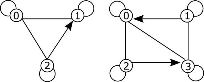
Figure 1: Examples of directed graphs that allow discrete time Quantum walks. Edges without arrows are undirected and can be traversed in either direction.

III Results

III.1 Probability flow

In order to analyse the locality of probability flows, it is helpful to break the probability current $J_{mn}$ (which represents the net flow of probability between vertices $n$ and $m$) into the individual flows of probability along the directed edges $n\rightarrow m$ and $m\rightarrow n$. In particular, we define the flow of probability along the edge $n\rightarrow m$ as $f_{mn}$. Then

$$J_{mn}=f_{mn}-f_{nm}.$$ (7)

Note that the ‘diagonal’ flow matrix element $f_{nn}$ corresponds to the amount of probability which remains at vertex $n$.

In order to give meaningful results and satisfy local probability conservation, the flow matrix elements $f_{mn}$ must satisfy the following properties:

$$f_{mn} \geq 0,$$ (8)

$$f_{mn} =0\quad\text{if}\quad n\rightarrow m\notin E,$$ (9)

$$\sum_{m}f_{mn} =P_{n},$$ (10)

$$\sum_{n}f_{mn} =P_{m}^{\prime}.$$ (11)

The first condition specifies that the probability flowing along an edge in a particular direction must be positive, the second that it must respect the locality structure of the graph. The third condition specifies that all probability initially at vertex $n$ must either flow to a neighbouring vertex or remain there during one time-step. The fourth condition requires that all probability at vertex $n$ after one time step must either have flowed to it from a neighbouring vertex or have remained there.

We now show that these properties for $f_{mn}$ yield all the required properties of $J_{nm}$. The flow $f_{nm}$ is a positive number hence $J_{nm}$ as defined in (7) is real. We also see that $J_{nm}$ is anti-symmetric, non-zero only when an edge exists between $m$ and $n$, and satisfies equations (5) and (6).

$$\Delta P_{n}+\sum_{m}J_{mn} =(P_{n}^{\prime}-P_{n})+\sum_{m}f_{mn}-\sum_{m}f_{nm}$$

$$=(P_{n}^{\prime}-P_{n})+P_{n}-P_{n}^{\prime}$$

$$=0$$ (12)

$$\sum_{m^{*}}J_{m^{*}n} =\sum_{m^{*}}f_{m^{*}n}-\sum_{m^{*}}f_{nm^{*}}$$

$$\leq\sum_{m}f_{mn}-\sum_{m^{*}}f_{nm^{*}}$$

$$\leq P_{n}.$$ (13)

Below, we show that a valid $f_{nm}$ satisfying properties (8)-(11) always exists, hence we can also define a valid $J_{nm}$ satisfying local probability conservation.

The converse is also true. If we can define a $J_{nm}$ which is real, antisymmetric, satisfies (5) and (6), and for which $J_{mn}>0$ only if $m\rightarrow n\in E$ then we can always generate flows $f_{mn}$ satisfying conditions (8)-(11). This is shown in the appendix, and illustrates that flow conditions (8)-(11) are equivalent to the conditions on the $J_{mn}$ given in the introduction.

III.2 Existence of local probability flows

To prove that we can define flow matrix elements $f_{nm}$ satisfying the conditions (8) to (11), we can use a result of Aaronson Aaronson (2005). However, for completeness and clarity, here we provide a simpler proof of a similar result which is sufficient for our purposes.

The key insight is to consider probability as a ‘fluid’, flowing through a network of ‘pipes’ with different capacities from a source to a sink. This can be described by a directed graph with edges which have a maximum capacity specifying the amount of probability allowed to flow along them. Figure 2 illustrates the configuration we will consider.

Figure 2: A diagram showing the movement of probability in the network flow picture. The line on the graph is an example of a cut. Vertices corresponding to $n\in A$ and $m\in B$ are shown half-filled.

This network consists of 3 different groups of edges. The first and final sets of edges have capacity corresponding to initial and finial probabilities respectively. The intermediate edges represent the evolution of the state and have capacity defined in the following way

$$C_{mn}=\begin{cases}0&\mbox{if }n\rightarrow m\notin E\\ 1&\mbox{otherwise}\end{cases}$$ (14)

If the total capacity of this network from source to sink is at least one, then for any flow configuration achieving capacity one the flow of probability along the edges in the middle section will give a valid $f_{mn}$. In particular, we set $f_{mn}$ equal to the flow of probability along the intermediate edge with capacity $C_{mn}$.

Following a similar approach to Aaronson (2005), we will show that the maximum flow allowed by the network is no less than one unit of probability by making use of the max-flow, min-cut theorem Dantzig (1964). This states that the value of the minimum cut in the network is equal to the maximum flow of the network. A cut is a set of edges which if removed from the network disconnects the source from the sink, and its value is the total capacity of those edges.

Let us first write down the value of a general cut. Let $A$ be the set of $n$ such that the edge $Source\rightarrow n$ is not in the cut and let $B$ be the set of $m$ such that the edge $m\rightarrow Sink$ is not in the cut. Then to disconnect the source from the sink the cut must contain all the edges $n\rightarrow m$ such that $n\in A$ and $m\in B$. Therefore the value of the cut can be written as

$$\sum_{n\notin A}P_{n}+\sum_{m\notin B}P_{m}^{\prime} +\sum_{n\in A,m\in B}C_{mn}$$

$$=(1-\sum_{n\in A}P_{n}) +(1-\sum_{m\in B}P_{m}^{\prime})+\sum_{n\in A,m\in B}C_{mn}$$

For our claim to hold the above expression must be greater than or equal to one. To show this we prove the following inequality

$$\sum_{n\in A}P_{n}+\sum_{m\in B}P_{m}^{\prime}\leq 1+\sum_{n\in A,m\in B}C_{mn}.$$ (15)

Firstly, we consider the case in which at least one of the $C_{mn}$ elements in the cut is non zero and secondly we consider the case where all of the $C_{mn}$ elements in the cut are zero.

In the first case, the right hand side of (15) is at least two. As any partial sum over elements of a probability distribution is at most one, the sum of the two terms on the left is at most two, and the inequality is satisfied.

In the second case, the right hand side of (15) is equal to one. In this case, it is helpful to express the left hand side of (15) in terms of projection operators as

$$\sum_{n\in A}P_{n}+\sum_{m\in B} P_{m}^{\prime}=\sum_{n\in A}|\bra{n}\ket{\psi}|^{2}+\sum_{m\in B}|\bra{m}U\ket{\psi}|^{2}$$

$$=\bra{\psi}\Big{(}\sum_{n\in A}\ket{n}\bra{n}+\sum_{m\in B}U^{\dagger}\ket{m}\bra{m}U\Big{)}\ket{\psi}$$

$$=\bra{\psi}\Pi_{A}+\Pi_{B}\ket{\psi}$$ (16)

where $\ket{\psi}$ is the initial state,

$$\quad\Pi_{A} =\sum_{n\in A}\ket{n}\bra{n}\quad\text{and }\quad\Pi_{B}=\sum_{m\in B}U^{\dagger}\ket{m}\bra{m}U.$$ (17)

$\Pi_{A}$ and $\Pi_{B}$ are projectors onto the spaces spanned by $\ket{n}$ such that $n\in A$ and $U^{\dagger}\ket{m}$ such that $m\in B$ respectively. In order to show that (16) is at most one, it suffices to show that $\Pi_{A}+\Pi_{B}$ is a projection operator.

$$(\Pi_{A}+\Pi_{B})^{2} =\Pi_{A}^{2}+\Pi_{B}^{2}+\Pi_{A}\Pi_{B}+\Pi_{B}\Pi_{A}$$

$$\Pi_{A}\Pi_{B} =\sum_{n\in A,m\in B}\ket{n}\bra{n}U^{\dagger}\ket{m}\bra{m}U=0$$

$$\Pi_{B}\Pi_{A} =\sum_{n\in A,m\in B}U^{\dagger}\ket{m}\bra{m}U\ket{n}\bra{n}=0$$

$$\implies(\Pi_{A}+\Pi_{B})^{2} =\Pi_{A}+\Pi_{B}$$ (18)

The cross terms go to zero as by assumption $C_{mn}=0$ which implies $U_{mn}=0\implies U_{mn}^{*}=0$. It is also clear that $(\Pi_{A}+\Pi_{B})^{\dagger}=\Pi_{A}+\Pi_{B}$. Hence $\Pi_{A}+\Pi_{B}$ is a projection operator and $\bra{\psi}\Pi_{A}+\Pi_{B}\ket{\psi}\leq 1$.

This shows that all cuts in the network shown in figure 2 have value greater than or equal to one. This then implies that the minimum cut in the network has value greater than or equal to one. Then by applying the Max-flow, Min-cut theorem we can conclude that the maximum flow allowed in the network is greater than or equal to one. As we only require one unit of probability to flow through the network at each time step this is sufficient to show that there exists a valid probability flow for every discrete time Quantum walk. Hence probability is locally conserved for quantum evolutions in discrete space time.

III.3 Constructing solutions

Although the above proof ensures the existence of a valid probability flow satisfying local probability conservation, it does not give a method of constructing such a flow. However, this can be achieved efficiently for cases with a finite number of vertices via linear programming.

If $N$ is the number of vertices in $V$, we can think of the flow matrix elements $f_{nm}$ as forming an $N^{2}$ dimensional real vector $\mathbf{f}$. The constraints (8)-(11) then correspond to a positivity constraint on each component of $\mathbf{f}$, and a number of linear equalities satisfied by the components. These can be expressed in the form

$$\mathbf{f} \geq 0,$$ (19)

$$\mathbf{A}.\mathbf{f} =\mathbf{b},$$ (20)

where $\mathbf{A}$ and $\mathbf{b}$ are a matrix and vector expressing the linear equalities (9) - (11). Given such constraints, a linear program can find a vector $\mathbf{f^{*}}$ which satisfies the constraints and maximizes the value of some linear objective function $c=\mathbf{v}.\mathbf{f}$. In this case, as we are only interested in finding a feasible assignment $\mathbf{f}$, it does not really matter what we choose as our objective function, but one natural choice would be to maximize the amount of probability which remains stationary (i.e. taking $c=\sum_{n}f_{nn}$). This would prevent probability from flowing in both directions between two vertices.

Various techniques exist to solve linear programming problems, including the simplex method Dantzig (1963), or Karmarkar’s algorithm Karmarkar (1984). The latter approach is efficient in the computational complexity sense, requiring a time which is polynomial in $N$.

III.4 Systems with Internal Degrees of Freedom

Quantum systems with internal degrees of freedom are commonly used in the context of coined quantum walks. In particular, we could consider a particle which carries an internal degree of freedom, such as a spin, in addition to its location. Alternatively we could consider cases in which each spatial location has its own distinct set of internal states.

In both of these cases we can denote an orthonormal basis of quantum states by $\ket{n,k}$ where $n\in V$ gives the spatial location and $k\in\mathcal{S}_{n}$ gives the internal degree of freedom. In such cases, we can apply the results obtained earlier, and thus prove local probability conservation, by mapping the system to one with no internal degrees of freedom. In this mapping, a vertex with $M$ internal degrees of freedom can be replaced with a set of $M$ vertices that are all connected to each other.

In particular, suppose that initially the different spatial locations form a directed graph with edge set $E\subseteq\{n\rightarrow m\,|\,n,m\in V\}$, then we can construct a new graph to represent the situation including the internal degrees of freedom, with vertices $V^{\prime}=\{(n,k)\,|\,n\in V,k\in\mathcal{S}_{n}\}$ and edge set $E^{\prime}=\{(n,k)\rightarrow(m,l)\,|\,n\rightarrow m\in E,k\in S_{n},l\in S_{m}\}$. For example any coined Quantum walk of a particle on a line with a two-dimensional degree of freedom is identical to a walk of a particle with no internal degrees on the graph shown in figure 3.

Local probability conservation on the expanded graph then implies local probability conservation for the original graph, with the probabilities and currents on the original graph being $P_{n}=\sum_{k}P_{(n,k)}$ and $J_{mn}=\sum_{k,l}J_{(m,l),(n,k)}$

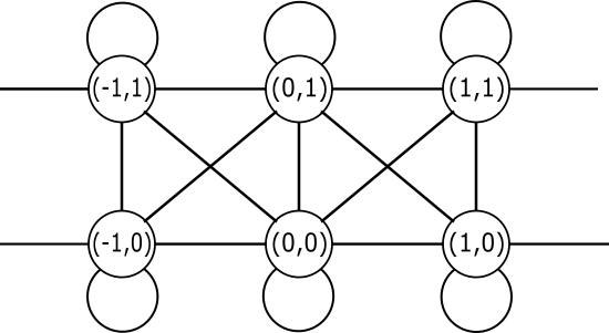
Figure 3: Any quantum walk of a particle on a line with a two dimensional internal degree of freedom can be represented by a quantum walk on this expanded graph. For generality, all links are shown undirected, allowing travel in both directions.

III.5 Mixed states and general quantum processes

So far we have considered pure quantum states evolving unitarily. However, it is also possible to extend these results to mixed states and general quantum processes (represented by completely positive trace preserving maps), which may be useful when considering open quantum systems or situations involving uncertainty. In this case the state is represented by a density operator $\rho$, and the transformation during a single time-step is given by $\rho^{\prime}=\sum_{i}K_{i}\rho K_{i}^{\dagger}$, where $K_{i}$ are Kraus operators Nielsen and Chuang (2011). In order to respect the locality structure of the graph, such a transformation must satisfy $n\rightarrow m\notin E\implies\bra{m}K_{i}\ket{n}=0\;\forall\,i$. Mixed states and general quantum dynamics can always be represented by pure states and unitary evolutions on a larger hilbert space composed of the original system and an ancilla Nielsen and Chuang (2011). By treating the ancilla as an internal degree of freedom as in the previous subection, it follows that local probability conservation also applies in these cases.

IV Discussion

For quantum evolutions in discrete space and time, in which the locality structure of space is described by an arbitrary directed graph and the evolution is unitary, we have shown that probability is locally conserved. Essentially, we can always explain the change in spatial probability distributions in terms of probability flows which respect the locality of space.

The constraint of local probability conservation can be expressed in terms of the probability current $J_{nm}$ between vertices or probability flows $f_{nm}$ along edges. Unlike in the continuous time examples which have been considered, the existence of a valid probability flow is established non-constructively, although valid solutions can be obtained efficiently via numerical methods.

A third approach to the probability flow is to consider a stochastic matrix $P_{m|n}$ which evolves the initial probability distribution into the final distribution via

$$P_{m}^{\prime}=\sum_{n}P_{m|n}P_{n},$$ (21)

with $n\rightarrow m\notin E\;\implies\;P_{m|n}=0$. This is equivalent to the formulation in terms of probability flows. To go from $f_{mn}$ to $P_{m|n}$ we take

$$P_{m|n}=\frac{f_{mn}}{P_{n}},$$ (22)

whenever $P_{n}\neq 0$. If $P_{n}=0$, (22) is not well defined. However, in such cases the distribution $P_{m|n}$ is irrelevant as there is no probability initially at $n$ to flow, and we can simply take $P_{m|n}=\delta_{m,n}$ to avoid violating the locality structure. Similarly we can transform from $P_{m|n}$ to $f_{mn}$ by taking $f_{mn}=P_{m|n}P_{n}$.

This result could be helpful in understanding quantum walk evolutions, and is also interesting from a foundational perspective, as it demonstrates that an intuitive property of quantum theory in continuous space and time and discrete space continuous time also holds in the discrete space and time formalism. This could be helpful for any approaches to particle physics in which discretization of time and space is pursued, such as Bialynicki-Birula (1994); Strauch (2006); Farrelly and Short (2014); D’Ariano and Perinotti (2014).

Appendix A Equivalence of flow and current conditions

In this appendix, we show that if we can define a $J_{nm}$ which is real, antisymmetric, satisfies (5) and (6), and for which $J_{mn}>0$ only if $m\rightarrow n\in E$ then we can always generate flows $f_{mn}$ satisfying conditions (8)-(11). As we showed in the main paper that these flow conditions always allow one to construct a probability current $J_{mn}$ with the specified properties this shows that these two sets of properties are equivalent.

To achieve this, we set

$$f_{mn}=\left\{\begin{array}[]{cl}J_{mn}&\mathrm{if}\,J_{mn}>0\;\mathrm{and}\;m\neq n\\ P_{n}-\sum_{m^{*}}J_{m^{*}n}&m=n\\ 0&\mathrm{otherwise}.\end{array}\right.$$ (23)

Property (8) is ensured by (6), property (9) follows because $n\rightarrow m\notin E\,\implies\,m\neq n\;\mathrm{and}\;J_{mn}\leq 0\,\implies\,f_{mn}=0$. The remaining two properties are given by

$$\sum_{m}f_{mn} =\sum_{m\neq n}f_{mn}+f_{nn}$$

$$=\sum_{m^{*}}J_{m^{*}n}+\left(P_{n}-\sum_{m^{*}}J_{m^{*}n}\right)$$

$$=P_{n}$$ (24)

$$\sum_{n}f_{mn} =\sum_{n\neq m}f_{mn}+f_{mm}$$

$$=\sum_{n:J_{mn}>0}J_{mn}+\left(P_{m}-\sum_{k:J_{km}>0}J_{km}\right)$$

$$=-\sum_{k:J_{km}<0}J_{km}+P_{m}-\sum_{k:J_{km}>0}J_{km}$$

$$=-\sum_{k}J_{km}+P_{m}$$

$$=\Delta P_{m}+P_{m}$$

$$=P_{m}^{\prime}$$ (25)