An Automated Engineering Assistant:
Learning Parsers for Technical Drawings

Abstract

From a set of technical drawings and expert knowledge, we automatically learn a parser to interpret such a drawing. This enables automatic reasoning and learning on top of a large database of technical drawings. In this work, we develop a similarity based search algorithm to help engineers and designers find or complete designs more easily and flexibly. This is part of an ongoing effort to build an automated engineering assistant. The proposed methods make use of both neural methods to learn to interpret images, and symbolic methods to learn to interpret the structure in the technical drawing and incorporate expert knowledge.

1 Introduction

Technical drawings are the main method in engineering to visually communicate how a new machine or component functions or is constructed. They are the result of a design process starting from a set of specifications that the final product needs to comply with. This design process follows a number of strict and soft rules (e.g., material choice as a function of temperature). Figure 1 shows a typical example containing both a 2D and 3D visualisation of the object, and a material list in tabular form specifying its parts and properties. They are carefully crafted documents that act as key deliverables at the end of a design process. As such, they contain a wealth of information. Furthermore, information is laid out according to generally applied conventions.

Engineering companies have a large database of previous designs, potentially going back decades. They are often underutilized because previous designs can only be searched for by title or by using a limited set of textual annotations. Ideally, however, this database can also be used to: (1) given a technical drawing, find other relevant drawings in a large database of previous designs; (2) given a partial description, find designs that would complete the partial design. In this work we present an approach that can extract the knowledge in a technical drawing and thus improve the search capabilities significantly to achieve the aforementioned tasks and assist engineers during the design process.

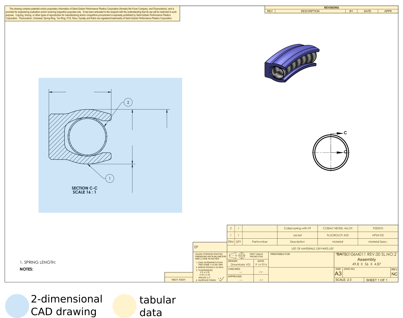
Figure 1: A technical drawing with highlights indicating the 2D CAD drawing and the tabular data

To be able to use the data encapsulated in technical drawings, we need to parse the information they contain, both tabular as well as visual, and translate this to a representation that can be handled by automated systems. Furthermore, such a system should be able to deal with both recent digital drawings and historical analog drawings. The latter is important because a great amount of information is captured in legacy drawings. Ideally, extracting the information can be done using a parser, which is a small computer program. The main challenge is that writing and maintaining such a parser is a time-consuming and expensive task. Furthermore, it is error prone since this requires an expert to explain subtle rules to an analyst or a programmer. The approach we present here will learn such parsers directly from expert feedback on the original drawing and allow its output to be used in automated tasks such as searching relevant designs.

Learning a parser requires expert input. Here, this input takes the form of annotated technical drawings. Providing such annotations is a trivial task for domain experts. The required number of drawings that need to be annotated is mainly dependent on the number of variations or templates that need to be recognized. Fortunately, since all technical drawings within an organisation are expected to be (loosely) based on a limited set of templates, the number of drawings that need to be annotated is also limited.

The approach presented in this work is a hybrid approach that utilizes both neural methods and reasoning-based methods. This combination is necessary to capture the full range of information. Neural methods such as deep convolutional neural networks are used because they are the state-of-the-art in image recognition algorithms. Despite their success, however, automatic analysis and processing of engineering drawings is still far from being complete [19]. This is in part due to the demand of neural methods for large amounts of training data. Such data is not always available, even though an expert might be capable of summarizing part of the knowledge or the parser in just a few abstract concepts. To exploit this expert knowledge, we also utilize reasoning based methods such as inductive logic programming and statistical relational learning. Such a hybrid approach that combines methods that are data-driven with methods that are knowledge-driven is gaining in popularity since real-world tasks tend to require Hybrid AI where human knowledge or reasoning is directly integrated [17, 18].

In this work we explain five contributions. First, we introduce the use of ILP to learn parsers from data and expert knowledge to interpret technical drawings. Second, we introduce a novel bootstrapping learning strategy for ILP. Third, we introduce a deep learning architecture that learns a meaningful summarization of CAD drawings. Fourth, we introduce a similarity measure to find related technical drawings in a large database. Finally, the efficacy of this method is demonstrated in a number of experiments on a real-world data set.

2 Overall system

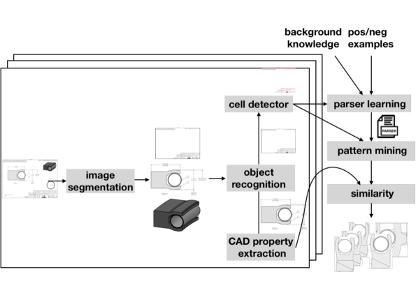
Figure 2: Overview of the technical drawing similarity proposal system.

The goal of extracting the key information contained in a technical drawing (e.g., Figure 1) is achieved by focusing our attention on two central components: (1) the tabular information with a list of parts and materials, author, date, etc.; and (2) the two-dimensional CAD-drawing visualizing the precise component shape and dimensions.

The modular structure of our implementation is shown in Figure 2. First, the central components of the drawing are extracted using image segmentation, and are identified by the object recognition module (Section 3). Then, we use the learned parser to extract properties from the tabular data (Section 4) and the CAD-drawing (Section 5). Finally, the output of these processing steps is synthesized into a feature vector on which we impose a similarity measure, over all possible designs (Section 6).

We had access to 5000 technical drawings, but used only the finished drawings. About $1\%$ of the drawings were unfinished (e.g. flagged as in progress, overlapping objects) and removed.

3 Identifying technical drawing elements

Archived technical drawings are digitized to varying degrees. Because of this, we consider as a baseline the case where the technical drawing is represented as a bitmap image.

3.1 Image segmentation

Extracting all the relevant elements contained in the image (e.g., tables, drawings) is achieved using conventional computer vision methods. The image is partitioned into its main segments using DBSCAN with $\epsilon=30$ and minimum points set to 0.001% of total pixels, thus $\approx 75$ points [11]. Since a technical drawing employs white space to distinguish central layout elements, such a density-based method is highly effective at segmenting images into their constituent elements. No errors were observed in the segmentation of the drawings.

3.2 Object recognition

Next, the system recognizes what each image segment represents by classifying them as one of three possible classes: ‘tables’, ‘two-dimensional CAD drawings’, and ‘irrelevant’ segments. This is a rather simple task as these classes are highly visually distinctive. High predictive accuracy is achieved with a small CNN classifier. For our implementation we relied on the PyTorch library [22]. This classifier was constructed with three convolution layers and three fully connected layers. It was trained against 318 technical drawings that were annotated by an expert, for a total of $3000$ image segments ($318$ tables, $372$ CAD drawings, $2310$ irrelevant segments). No classification errors were made on a test set of 53 technical drawings containing 500 segments.

In case a table is recognized we apply one additional operation to identify the cells by applying a contour detection algorithm [28] provided by the OpenCV library. The cells of each table are subsequently processed by the parser learning-module, which is specifically aimed at learning how to read the tables contained in the technical drawings referenced throughout this paper, such as a material bill (see Section 4). In case a 2-dimensional CAD drawing is recognized, the image data is passed on to the CAD property extraction-module that has learned how to recognize the application dependent parts of an image (see Section 5).

4 Extracting properties from tables

The data contained in a technical drawing is laid out in a manner that facilitates human interpretation. Tabular data in particular tends to be organised both spatially and through explicit annotation. Common examples of spatial structuring involve assigning related cells to common rows or columns, while assigning unrelated cells to different subtables or distant cells. Particularly useful are cells that contain unambiguous keywords such as attribute names. These are helpful to gain insight in the structure of a table. They serve as anchors to cells that are less distinctive on their own but can easily be described relative to them.

The application at hand does not only require us to parse a table, but also demands that we learn how to interpret its spatial organisation. A small computer program is required to parse these custom drawings. Programming a parser for each type of drawing is not only an expensive and time consuming task to build and maintain, but also error-prone. Various errors are potentially introduced while programming a parser. First, the structure of such technical drawings needs to be explained to a non-expert, i.e. a programmer, who interprets the instructions. Second, the tables are typically not simple rectangular tables. They thus require a non-trivial parser that is difficult to understand. Third, a design can deviate slightly or change over time requiring periodic maintenance and potentially leading to software erosion. Ideally these programs would be derived directly from the expert’s knowledge, and be easily updated when new designs appear. This is possible by means of machine learning techniques that learn programs from examples. The examples in this setting are obtained by annotating technical drawings, a task that is trivial for a domain expert.

The highly relational nature of tabular data and the ease with which tables can be sensibly navigated by visiting adjacent cells suggests the use of Inductive Logic Programming (ILP). ILP systems are particularly suitable for learning small programs from a limited amount of complex input data. When learning the programs covered in this work using ILP, we benefitted in particular from the ability to learn recursive definitions (e.g., row $n$ is defined by row $n+1$) and reuse learned target labels (e.g., first learning what a header row is helps to define what a content row is). A logic program consists of a set of definite clauses. A definite clause can be interpreted as a rule. One such definite clause might look like: $h(a,X):-b_{1}(a,X),b_{2}(X).$ where $h(a,X)$, $b_{1}(a,X)$, and $b_{2}(X)$ are literals whose arguments can either be constants or logical variables. Constants are denoted using lowercase letters or numbers, while variables are uppercase letters. Disjunction is represented using ‘;’ and conjunction using ‘,’. Programs obtained through ILP can be augmented with probabilistic distributions. This combination is referred to as Statistical Relational Learning [13, 7] and can naturally deal with uncertain input information. This is a useful property, because the input data for the parser is provided by other machine learning models. For example, the OCR engine returns a distribution over characters instead of a 100% certain prediction.

4.1 Inductive Logic Programs for Parsing

An inductive logic programming system learns from relational data a set of definite clauses. Given background knowledge $B$, positive examples $E^{+}$ and negative examples $E^{-}$, it attempts to construct a program H consisting of definite clauses such that $B\wedge H$ entail all, or as many as possible, examples in $E^{+}$, and none, or as few as possible, of those in $E^{-}$.

We thus need to supply three types of inputs.

First, a set of training data, examples $E$, that contains the properties to describe a cell in a technical drawing. An example can be:

• Cell text: The textual contents of each cell. Tesseract 4.0 is used to recognize cell contents [25].

• Cell location: The cell’s bounding box information (i.e. (x,y) coordinates and cell width and height).

Second, a label for each cell (e.g., author, bill of materials, quantity). A cell can be annotated with multiple labels (e.g., a cell can be a quantity in the bill of materials). Depending on which target label we want to learn, we split the set of examples $E$ in a tuple $(E^{+},E^{-})$ where $E^{+}$ contains the examples associated with a cell that has the target label and $E^{-}$ those examples that do not. For standard ILP, the learning task is defined for one target label, so we repeat the standard ILP task for each label in the set of labels.

Third, we can provide background knowledge $B$ that contains generally applicable knowledge for the problem at hand and remains unchanged across examples. In this case we provide:

• Relative cell positions. Relations capturing which cells are adjacent to each other, and in which direction (horizontally or vertically) based on their bounding boxes.

• Numerical order. The successor relationship. Although not essential, it is useful for learning concise, recursive rules.

The output of ILP, the program $H$, is a set of definite clauses of the form ‘author(A) :- cell_contains(A, drawn)’ which can be read as the rule: Cell A contains the author if it contains the word ‘drawn’.

4.2 ILP with bootstrapping

It is expected that learning programs to properly parse the target labels in P will prove simple for some targets and more challenging for others. We propose a bootstrapping extension that supports the construction of sophisticated programs by allowing them to employ the simpler ones in their definition. This is loosely inspired by the ideas raised in [8], but applied to the ILP setting.

This corresponds to a variation of the previously discussed ILP set-up where a dependency graph $G$ is used. The nodes in this directed acyclic graph each represent a possible target label and the edges represent dependencies between those labels. A dependency indicates that one target label might have a natural description in function of another. Although we allow for this dependency graph to be specified manually, our method defaults to a fully automated approach where standard ILP is first applied to learn programs for each target. Then targets are ranked according to, first, ascending $F_{1}$ score on the training data and, second, the size of the program in number of literals. Each target in the ranking then has all subsequent targets as its dependencies. Finally, ILP with bootstrapping learns targets in the order specified by a correct evaluation order of $G$, and extends the background knowledge $B$ for each target with the programs constructed to parse its dependent target labels. When learning program H using bootstrapping to capture a particular target label l, we define its extended background knowledge $B^{\prime}=B\wedge(\bigwedge_{i\in descendants(G,l)}H_{i})$, where $H_{i}$ is the program trained for target label i.

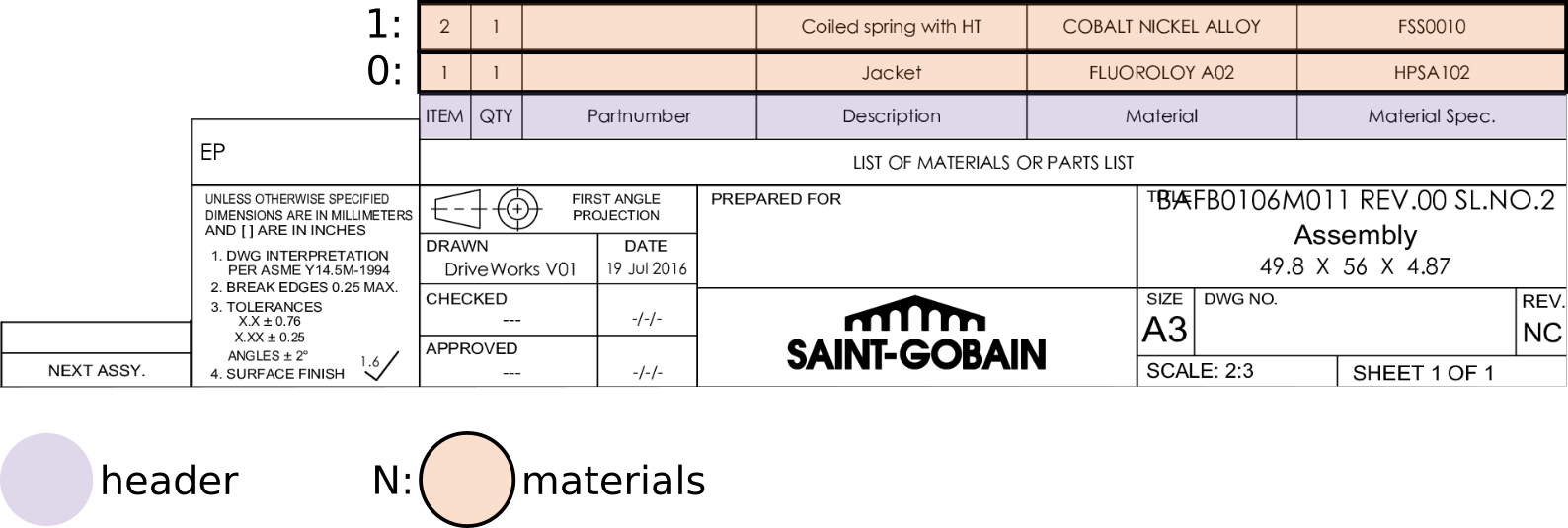
(a) A table excerpt from a technical drawing. Its header and materials are highlighted.

⬇

% Materials hypothesis

materials(A,B) :-

zero(A),

above_below(B,C),

header(C).

⬇

materials(A,B) :-

succ(C,A),

above_below(B,D),

materials(C,D).

⬇

% Header hypothesis

header(A) :-

above_below(A,B),

cell_contains(B, ‘LIST’).’

(b) header/1 covers any cell located directly above a cell containing the word ‘LIST’. materials/2 parses the indexed parts of the materials table. Its first argument is the index and its second argument represents the cell. materials/2 consists of two clauses. The first clause anchors the table by considering row 0 to consist of the cells above the header. It employs header/1 in its definition. The second, recursive clause indicates that the index is incremented whenever a row is located above another.

Figure 3: Figure 3(a) provides an illustration of the materials table and its header. Listing 3(b) shows the associated program learned using bootstrapping.

4.3 Experiment set-up

The ILP system Aleph [26] is used to learn possibly recursive programs that parse the chosen targets from the tabular data, ranging from the document’s author and its approval date to the attributes covered in the materials table and its indexed components.

Training data consists of a set of fully labeled technical drawings. A custom data labeling tool with a web-based graphical interface was constructed to support domain experts in labeling drawings.

Using this tool, 30 technical drawings with on average 50 cells were labeled with 14 different labels. For each target label, examples that contain that label form its positive example set, while negative examples are automatically derived by taking the complement of all possible examples for that target with its positive example set.

The labeled data is split in a training set consisting of 10 drawings, and a test set containing the remaining 20. Since the choice of training data can heavily affect the capability for finding rules that properly generalize, experiments are repeated 5 times on random samples of the training data. Because the order in which training examples are presented can also affect the rules identified by the coverage-based algorithm employed by Aleph, repeat experiments are performed even when all training data is available for learning, as a sample then corresponds to a different order in which the examples are presented to the learner.

When inducing programs using Aleph, we employ a proof depth of 12, a clause length of 5, and an upper bound of 60 000 on the number of nodes that may be explored during clause learning. Note that these settings have to be selected with care. Since several of the learned programs employ recursion, a too restrictive proof depth can cause the learner to incorrectly conclude that a candidate program has failed to cover a training example. This would result in the addition of at best redundant, and at worst harmful clauses. A bound on the proof depth is nevertheless a necessity, as not all candidate programs are guaranteed to terminate.

4.4 Results

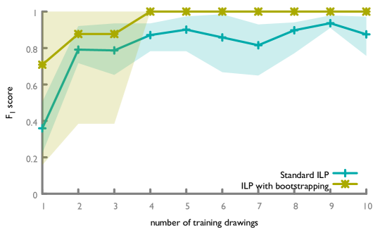
Figure 4: The performance measured using the $F_{1}$ score of programs learning materials/2. Min/max shading is included to indicate the range of performance between the best and worst-performing program over 5 repetitions.

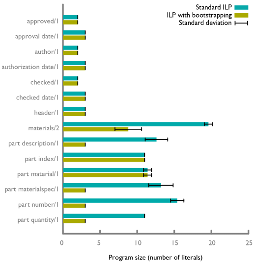
Figure 5: The difference in average program size (measured in number of literals) between standard ILP and ILP with bootstrapping across programs induced on 14 labels. 10 repetitions were performed on a training set of 20 labeled drawings.

Figure 4 visualizes the performance with which cell labels and their appropriate index are correctly identified. This shows that only a few annotated designs are required for the bootstrapping method to learn perfect parsers for all labels whereas the standard ILP approach fails to learn a perfect parser. Furthermore, it highlights how ILP with bootstrapping compared to Standard ILP is less sensitive to overfitting when presented with additional training data. This robustness of ILP with bootstrapping lends itself well to incremental learning. Both subtle and drastic variations in template design can be handled by providing the learner with a representative sample as training data.

We have observed that learning perfect parsers for simple labels such as author or approval date can be achieved by both standard ILP and the bootstrap method with only a few training examples. More interesting is to look at the most complicated label, the indexed components (materials in Figure 3(a)).

The best performing program constructed using standard ILP in Figure 4 consists of 14 clauses and yields 17 false negatives. Bootstrap learning, however, succeeds at learning a completely accurate, concise program whenever more than three technical drawings are provided in the training set. The poor performance when using only a few drawings is due to poor generalization. More specific, in these drawings the materials tables provided for training each consisted only of a single row in addition to the header, and there was no pressure on the inductive learner to learn the recursive rule necessary to capture the rows of larger tables.

A comparison of program size between Standard ILP and ILP with bootstrapping across all investigated labels is shown in Figure 5.

4.5 Statistical Relational Learning for Uncertain Input

The insights gained while learning the structure of the technical drawing using ILP can be leveraged to improve the knowledge extraction process. Here we examine two improvements where the output of the optical character recognition (OCR) software is improved by augmenting it with contextual knowledge. An issue is that the knowledge learned by ILP is deterministic while the results from OCR are probabilistic (i.e. a distribution over possible characters). A natural generalization of ILP is Statistical Relational Learning which combines logic formulas with probabilities. We use ProbLog, a probabilistic logic programming language, to extend the learned ILP programs to be able to cope with probability distributions.

4.5.1 Probabilistic Levenshtein distance

The content of many cells in a technical drawing are drawn from a predictable set of characters, and in some instances even from a specific set of strings. The employees involved in authoring a document are for instance likely to be present in an existing database. By explicitly establishing such a link, we can not only improve the quality of the text recognition, but also identify diacritics that are lost when names are for example displayed using upper-case representations, and avoid, or more easily identify and resolve ambiguity. While the Levenshtein distance is a suitable metric for identifying the similarity of pairs of strings, it fails to account for the probabilistic nature of our data. As such, we consider a generalization implemented in ProbLog that applies the Levenshtein distance to a probabilistic input string (see Listing 1). The algorithm is similar to the implementation of Levenshtein using the Viterbi decoding except that penalties are expressed as probabilities, i.e. the probability of a transition in the Viterbi lattice, and the input is represented as a probability distribution over possible characters on each position in the string.

Listing 1: A ProbLog program that performs a probabilistic Levenshtein distance (note that selecting the max-product semiring in ProbLog for this program achieves a probabilistic implementation of the Viterbi decoding version of the Levenshtein algorithm).

⬇

% OCR probability distribution

0.8::$c_{o}$(0,d); 0.1::$c_{o}$(0,b); 0.1::$c_{o}$(0,o).

$c_{o}$(1,r). $c_{o}$(2,i).

0.8::$c_{o}$(3,e); 0.2::$c_{o}$(3,3).

$c_{o}$(4,s). $l_{o}$(5).

% Probabilistic Levenshtein Distance (pld)

pld(_,-1,-1).

0.3::pld(W,R,C) :- % Insertion

R>-1,C>-1, Rp is R-1,

pld(W,Rp,C).

0.3::pld(W,R,C) :- % Deletion

R>-1,C>-1, Cp is C-1,

pld(W,R,Cp).

pld(W,R,C) :- % Match

R>-1,C>-1, Rp is R-1, Cp is C-1,

nth0(R, W, CW), $c_{o}$(C, CO), CW=CO,

pld(W,Rp,Cp).

0.3::pld(W,R,C) :- % No match

R>-1, C>-1, Rp is R-1, Cp is C-1,

nth0(R, W, CW), $c_{o}$(C, CO), CW\=CO,

pld(W,Rp,Cp).

pld(W) :- % Entry point

length(W, WL), $l_{o}$(OL),

WLp is WL - 1, OLp is OL - 1,

pld(W, WLp, OLp).

% Query

query(pld(wannes)). % Pr = 0.05

query(pld(dii3s)). % Pr = 0.26

query(pld(dries)). % Pr = 0.77

4.5.2 Type-information enhanced OCR

As a second use case we examine how integrating type-information can augment text recognition. The concept is illustrated on a cell in the quantity column of the materials table. Such a cell indicates the frequency with which its associated part occurs within a design.

In our tests, text recognition frequently confused characters like ‘0’ with ‘O’, and ‘1’ with characters such as ‘]’ and ‘I’. Such ambiguity is generally resolved through the use of dictionaries, or by training the OCR software against the exact font used in the example image. In the quantity column however, characters occur in isolation, and even in the rest of the table they frequently appear as part of complex identification codes. This renders publicly available dictionaries useless. Furthermore, the robustness of the system demands high performance even when the employed font is unknown.

Our proposed solution involves taking into account our expectation of the type of data contained in a given cell. There exists for example a high degree of confidence that the quantity column contains numerical information. Since we now have the means to learn a program that identifies these elements, the remaining challenge involves deciding on how to combine this information. [4] present a solution using virtual evidence. The virtual evidence method considers an original distribution over events $\alpha$ (The distribution over characters based on our understanding of the type information) which is put up for revision based on some uncertain evidence $\eta$ on a set of mutually exclusive and exhaustive events $\gamma$ (the distribution over the set of characters returned by the OCR software). It finds that virtual evidence can be incorporated using Bayes’ conditioning.

$$P(\alpha|\eta)=\frac{\sum_{i=1}^{n}P(\eta|\gamma_{i})P(\alpha,\gamma_{i})}{\sum_{j=1}^{n}P(\eta|\gamma_{j})P(\gamma_{j})}$$

The set of events $\alpha$ has a one-to-one mapping with $\gamma$ as they span the same set of possible characters. Since $P(\alpha,\gamma_{i})=P(\alpha|\gamma_{i})P(\alpha)$, we can conclude that $P(\alpha|\gamma_{i})$ corresponds to the Kronecker-$\delta$ over $\alpha$ and $\gamma$. As such we find that the numerator consists of the conjunction of the distribution returned by the OCR software and the distribution established by the type information, while the denominator acts as a normalizing term. A ProbLog program [12] representing virtual evidence applied to a particular cell of the quantity column is shown in Listing 2, and its associated distributions are explicitly shown in Figure 6

Listing 2: A ProbLog program that augments a given distribution $c_{k}$ using uncertain evidence $c_{o}$

⬇

% For conciseness, we explicitly model $c_{k}$/1 as

% the prior distribution established by the

% type information (here, restricted to characters

% used by $c_{o}$).

% Normally, an implicit representation using rules

% would be employed

% e.g. [numerical:0.8, alphabetical:0.1, special:0.1]

0.615::$c_{k}$(1) ; 0.077::$c_{k}$(2) ; … ; 0.077::$c_{k}$(]).

% OCR probability distribution

0.630::$c_{o}$(]) ; 0.130::$c_{o}$(1) ; 0.071::$c_{o}$(|) ;

0.071::$c_{o}$(I) ; 0.054::$c_{o}$(J) ; 0.043::$c_{o}$(l).

% Revising the distribution derived from

% the type-information by taking the conjunction

% with the OCR probability distribution

q(X) :- $c_{k}$(X), $c_{o}$(X).

% Setting the evidence

e :- q(X). % one of them should be true (i.e. ’there

% exists an answer that satisfies the query’)

evidence(e).

% Query

query(q(X)).

(a) A cell containing ‘1’.

symbol OCR distribution OCR + type information uncertain evidence prior posterior 1 0.130 0.615 0.544 ] 0.630 0.077 0.330 $|$ 0.071 0.077 0.037 I 0.071 0.077 0.037 J 0.054 0.077 0.028 l 0.044 0.077 0.023

(b) Distributions over symbols for the identification of a single character

Figure 6: OCR is applied on the displayed cell. While the most likely candidate symbol according to the OCR distribution is the square bracket, the posterior correctly considers ‘1’ to be the most probable symbol. Here, the prior distribution is defined only over those characters that appear in the OCR distribution.

5 Extracting properties from CAD visualisation

Some aspects of a design can only be communicated by sharing a visual depiction. This concerns for example the subtleties of component shapes, and the exact manner of their assembly. These features can prove essential in distinguishing designs that have identical tabular information (e.g., material choices), and as such can be vital to construct a comprehensive representation of the technical drawing.

A technical drawing tends to contain both a 2D and 3D depiction. We consider the 2-dimensional CAD drawing as the most suitable target for visual analysis as the profile view offers a clear, uncluttered view of the design.

5.1 Learning key identifiers from unlabeled data

Many of these visual features of interest are only present in the CAD drawing and cannot be linked to features in the table or in the meta-data. This means we cannot apply standard supervised learning because there are no labels available. However, this is not a problem since we are mainly interested in learning what the relevant features are that can identify designs. Not yet what type of design it is. The goal will thus be to learn a limited set of features that are expressive enough to uniquely identify designs, can generalize over different designs, and remain unaffected by translations or rotations of the design.

We propose to transform the problem to a binary classification task that captures these requirements. Given a pair of 2-dimensional CAD drawings, a classifier with a limitation on the numbers of features is trained to predict whether the pair represents the same design or not. If the classifier achieves high accuracy on this task we consider the set of learned features to fit the requirements and we will use this set of features in a next step to summarize each design.

The data set for these input pairs is constructed as follows. For each of the 2-dimensional CAD drawings available to us, we generate 10 variations by applying arbitrary flips, rotations and translations. We consider this image set consisting of 11 images to be representative for each design. The data for the ‘same’ class is then formed by considering every pairing within each image set, while the ‘different’ class is constructed by sampling an equal number of pairs across image sets. This ensures the resulting data set is balanced.

5.2 CNN architecture and setup

Neural networks are widely known for their capability of capturing complex and non-obvious properties of the data they are trained with. Convolutional Neural Networks (CNNs) are a category of neural networks of particular interest, as they have seen wide adoption in image recognition and classification. They are classifiers whose key characteristic is their usage of convolutional layers. An input image is passed through a series of such layers. Each layer consists of convolved features (i.e., the neurons) by applying a kernel on parts of its input. While the features captured in early layers are limited to angled edges and simple blobs, they become increasingly more complex as the layers deepen, until they are capable of describing domain-specific elements.

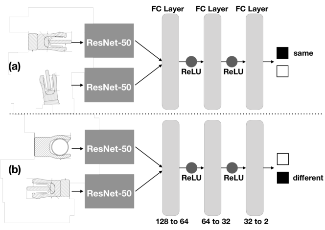
Figure 7: The ResNet-50 block consists of a ResNet-50 architecture where its final fully connected (FC) layer maps its 2048 inputs to a layer of size 64. This layer represents the set of derived features, i.e., the visual features of interest.

Convolutional neural networks have a proven capacity to learn complex features (i.e., representation learning). The challenge is to identify those that match our requirements. Notably, we find that the classification task outlined in Section 5.1 can directly be integrated in a CNN architecture, allowing it to learn features that are optimized to score well on the classification task.

Figure 7 shows our CNN architecture. The ResNet-50 [14] architecture is used to perform the various convolutions. Since the features identified in the pre-trained model are tailored to a wide set of common settings, while ours is a very domain-specific, we re-train only the last layer to tailor the derived features to our data. While the output layer of ResNet-50 has size 1000, we map it to a layer of size 64. This layer corresponds to the relevant features that will be used to identify design. The rest of the architecture is constructed in order to effectively classify the input image pairs into one of the two possible classes: ‘same’, or ‘different’. Note that the same ResNet-50 network is used to encode both images. The expectation is that the CNN to be attentive of visual features of varying detail, as the visual differences between seals can vary from striking to intensely subtle. Our classifier achieves a 96.8% accuracy at this task (training set: 68,507 pairs, validation set: 34,253 pairs, test set: 68,507 pairs).

5.3 Experimental results

5.3.1 t-Distributed Stochastic Neighbor Embedding (t-SNE)

(a) perplexity 20

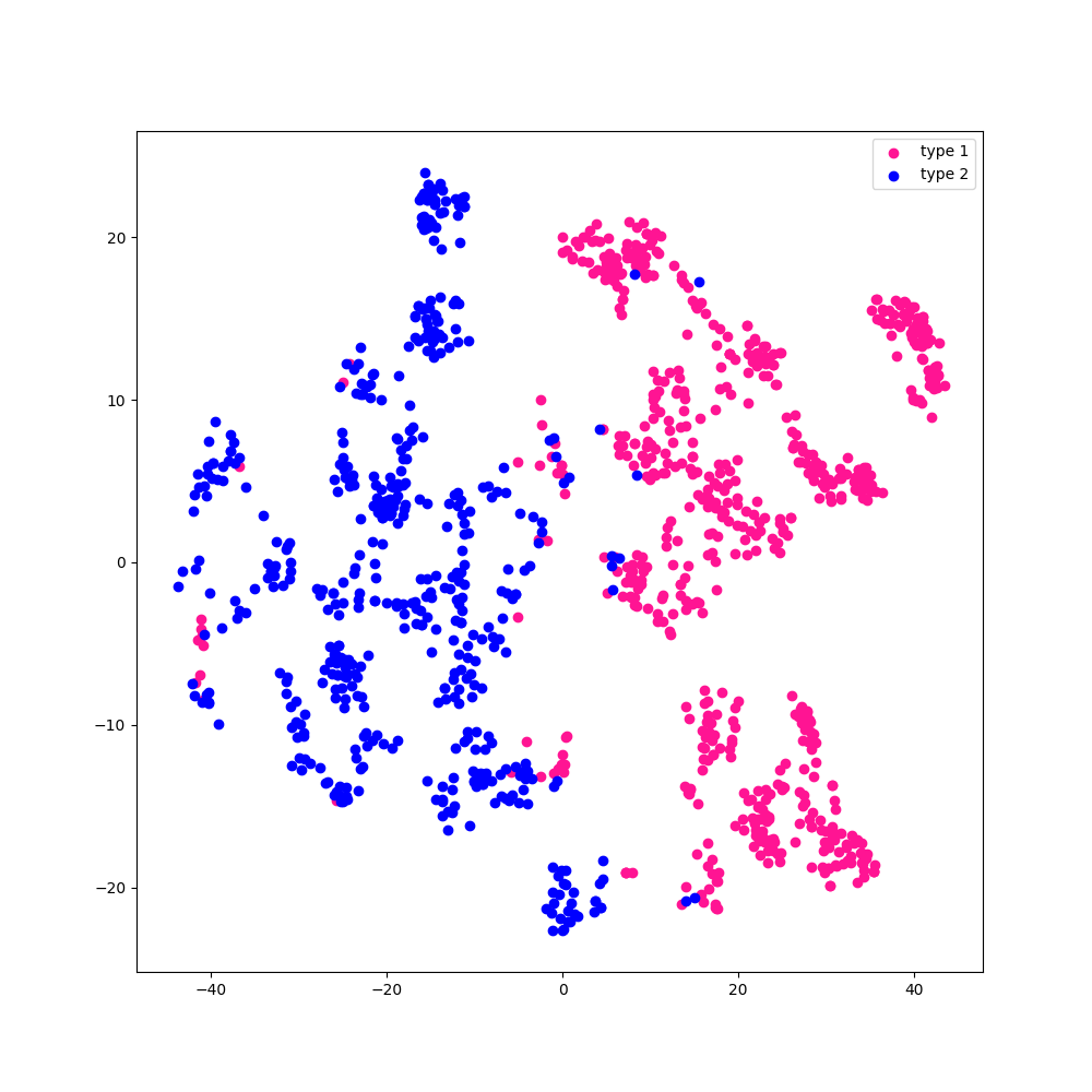
(b) perplexity 50

(c) perplexity 100

Figure 8: t-SNE visualisation over 2 components for varying values of perplexity.

We can now apply the CNN network to all drawings in the database and construct a feature vector from the 64 relevant features, thus the neurons in the last layer of our ResNet-50 model. Figure 8 shows a t-SNE visualisation for varying values of perplexity of the features vectors for each of the drawings in our dataset. The data points are colored according to an expert labeling which groups designs according to properties deemed to have a high visual impact. This labeling has two values with high representation, and the visualisation clearly separates them in distinct, non-overlapping clusters. Since our interest lies in the detection of novel features, being able to identify a pre-existing one is not actually our goal. However, since a failure to visually distinguish between these types would falsify our hypothesis that we are extracting meaningful visual data, this result does inspire confidence.

5.3.2 Gradient-weighted Class Activation Mapping (Grad-CAM)

This belief is strengthened further when analyzing the behaviour of the CNN using Grad-CAM [24]. Grad-CAM provides a coarse localization map of the important regions in the image. We find that our derived features focus their attention on image regions that correspond to meaningful properties in our application domain. Figure 9 visualizes a selection of the derived features activating in the presence of a particular type of ring seal.

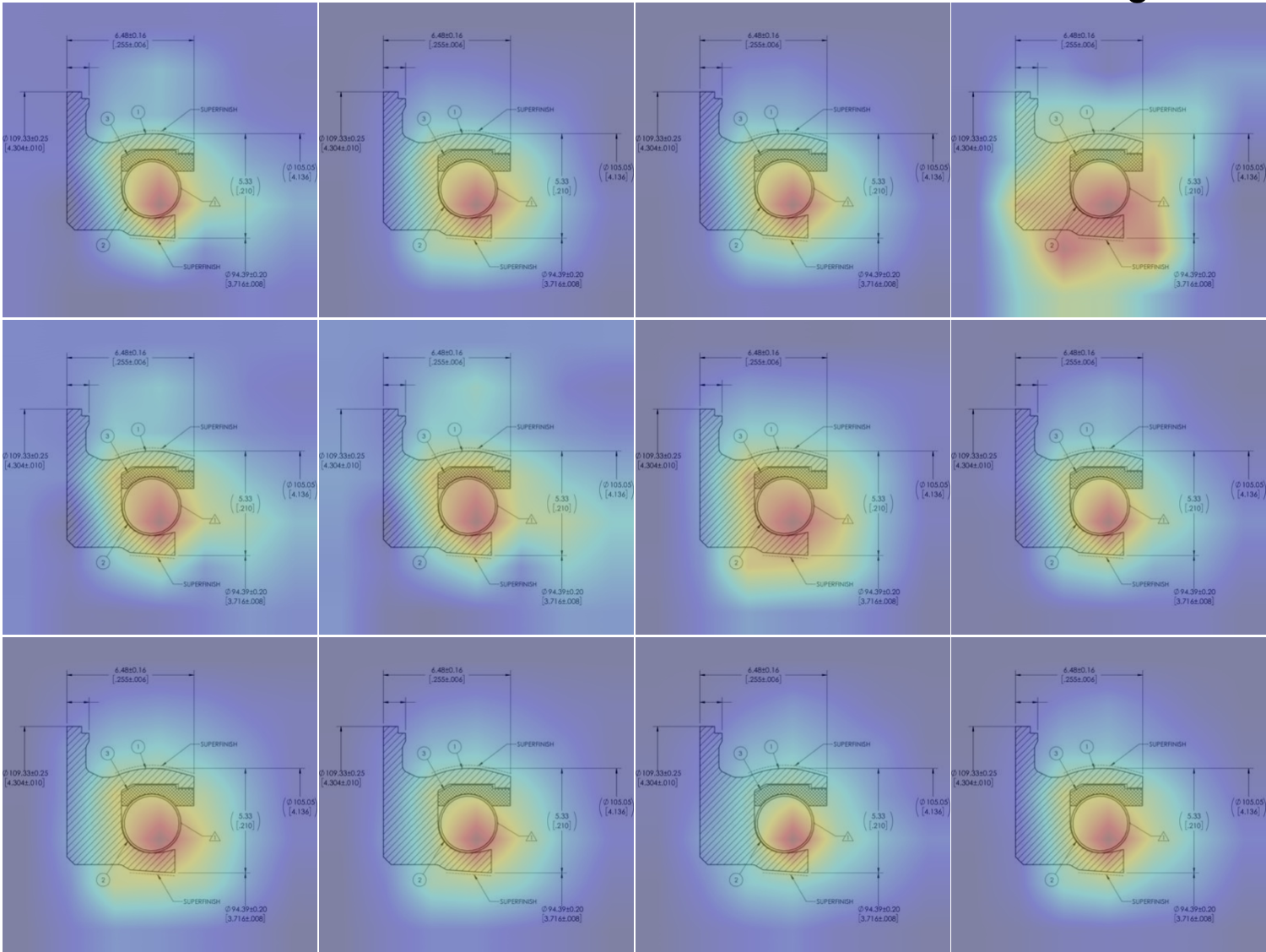
Figure 9: A Grad-CAM visualization. Warmer areas correspond to regions that play a more significant role in the activation of a derived feature. Here, each image depicts a derived feature whose attention seems largely focused on the ring of the seal

6 Identifying relevant designs

Using our results from Section 4 and 5, we now have access to the design properties contained in both the tabular data and the visual depiction of the seals. In order to leverage these results when suggesting relevant designs, we will first impose a similarity measure on them separately, and then combine the resulting similarity measures using a weighted geometric mean.

6.1 Tabular data similarity

Due to its highly relational nature, it is not feasible to directly apply a conventional similarity measure to the tabular data. Instead, we first propositionalize the data using Frequent pattern (FP) mining. FP mining has shown to be effective at this task [15].

Listing 3: Three frequent patterns mined using WARMR

⬇

% A design has a part that uses the words

% ‘Double’ and ‘NICKEL’ in its cells.

materials(B,A),cell_contains(A,‘Double’),

materials(B,C),cell_contains(C,‘NICKEL’).

% A design has a part that includes

% the word ‘COBALT’ in one of its cells,

% and also employs the word ‘Spring’

% in its description column.

materials(B,A),cell_contains(A,‘COBALT’),

materials(B,C),part_description(C),

cell_contains(C,‘Spring’).

% A design contains the words ‘Jacket’,

% ‘Spacer’, and ‘Spring’ in its

% description column.

part_description(A),cell_contains(A,‘Jacket’),

part_description(B),cell_contains(B,‘Spacer’),

part_description(C),cell_contains(C,‘Spring’).’

We perform FP mining using WARMR [9] on the tabular data extracted in Section 4. We focus on retrieving patterns that occur in $\geq 10\%$ of the drawings. Listing 3 shows a sampling of the resulting patterns. In total we mined 9120 such patterns. Each technical drawing is then represented as a binary vector indicating which patterns are applicable. Given such a vector representation, closely related designs can be identified by performing a ranking using the complement of its normalized Hamming distance to all other designs.

Given two drawings represented as binary vectors X and Y

$$\textit{sim}_{\textit{tabular}}(X,Y)=1-\frac{1}{n}\sum_{i=1}^{n}|X_{i}-Y_{i}|$$

6.2 Visual similarity of seals

In Section 5 we discussed how the final fully connected layer of our ResNet-50 architecture captures key visual properties of a seal using a layer of size 64. All the features in this layer are continuous. The expectation is that the features of visually similar seals have similar values. Cosine similarity against this set of derived features is used to determine similarity.

Given two drawings represented as feature vectors X and Y

$$\textit{sim}_{\textit{visual}}(X,Y)=\frac{X\cdot Y}{||X||_{2}\cdot||Y||_{2}}$$

6.3 Ranking designs by similarity to a given design

Tabular data similarity and visual similarity are combined using a weighted geometric mean.

$$\prod_{i}\Bigl{(}x_{i}^{w_{i}}\Bigr{)}^{1/\sum_{i}w_{i}}$$

The use of a geometric mean ensures that the resulting similarity is not biased towards a particular one of its constituent similarity measures due to the distribution of their values, but rather accounts only for the relative changes to each score across designs. The use of a weighted mean makes the inherent trade-off between potentially conflicting measures explicit.

Here, we use this convex combination solely to combine tabular data similarity and visual similarity. This trade-off can be captured in a single parameter $\alpha$ such that

$$\textit{similarity}={(\textit{sim}_{\textit{tabular}})}^{\alpha}\cdot{(\textit{sim}_{\textit{visual}})}^{1-\alpha}$$

In doing so, users can easily impose their own biases and preferences to influence the ranking. In our implementation we use $\alpha=0.5$. Figure 10 shows a depiction of some of the designs ranked given a particular technical drawing.

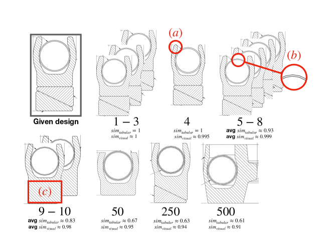
Figure 10: A depiction of a number of designs annotated with a rank indicating their similarity to the highlighted design ($\alpha=0.5$). Subtle though significant differences are seemingly picked up, while insignificant though sizable differences in shading seem to have little to no effect. The lip of the seal in (a) differs from the original, possibly explaining the difference in its $sim_{visual}$ score. The ring in (b) appears as a polygon instead of a circle, and the body of (c) consists of a single contiguous part as opposed to multiple elements separated by a diagonal.

6.4 Ranking designs by similarity to a given partial design

The ability to identify similar designs is particularly useful when applied to a design under construction. If such a design displays high similarity to existing ones, the most similar ones can provide the engineer with possible completions.

We consider a partial design to be represented as a technical drawing containing a number of empty cells. During property extraction, the cell text of empty cells is represented using logical variables.

If a visual depiction of the seal is present, $sim_{visual}$ can be computed as usual. If it is omitted, the similarity measure is restricted to its $sim_{tabular}$ term.

As a consequence of allowing the inclusion of empty cells, some of the patterns employed by the feature vector used to construct $sim_{tabular}$ might not have a proper instantiation on the partial design. Given T the set of all properties of the partial technical drawing, we distinguish three situations:

• True. A feature is true on the partial design when each of the literals in its conjunction have a corresponding match in T that does not require the instantiation of any logical variable in T.

• False. A feature is false on the partial design if at least one of the literals in its conjunction fails to find a corresponding match in T.

• Unknown. Any feature for which it is not known whether it is True or False.

$sim_{tabular}$ against a given partial design can then be computed by utilizing feature vectors that are filtered to contain only those features that were True or False on the partial design.

7 Related Work

7.1 Digitisation of technical drawings

Two recent papers cover the domain of document digitisation. First, [27] shows significant progress digitising general PDF and bitmap documents. Second, [20] provides an overview of all recent trends on digitising engineering drawings in particular. The work of [27] focuses on detecting elements in text documents in general and parses tables but cannot take easily into account expert knowledge to achieve near perfect extraction for specific cases or extract information embedded in figures.

With regards to shape detection, [20] makes a distinction between specific approaches focused on identifying shapes that are known in advance, and holistic approaches where the underlying rules of the drawing are exploited to split it into parts. Our approaches for identifying technical drawing elements utilized a mixture of both. The use of image segmentation and text detection in Section 3 falls under the holistic view, while the contour detection in Section 3.2 is an illustration of a specific approach. While [20] notes that some frameworks do perform contextualisation (i.e., inferring and exploiting the relationship between symbols within drawings), our approach is to our knowledge the first that enables the construction of a comprehensive, formal representation of a technical drawing that supports the inclusion of expert knowledge that is obtained by learning an interpretable parser that takes into account expert knowledge and can identify unique properties in drawings.

7.2 Feature extraction

While established feature extraction methods such as SIFT [16] and SURF [2] are still viable alternatives, CNNs are increasingly the go-to method when extracting features. Industrial applications of CNNs are however strongly limited by the cost of collecting a suitable set of labeled training data [20]. Our approach side-steps this issue by learning from unlabeled data through the introduction of a discriminative setting. This approach is comparable to that of Exemplar-CNN [10].

In this work, autoencoders were observed to perform poorly as a means to capture features. When encoding an input image to a lower dimensional feature space, an autoencoder seeks to capture as much of the input data as possible with the aim of later on reconstructing the image as faithfully as possible. Here however, most of the input data proves to be irrelevant. The exact position and rotation of a seal is completely irrelevant, and even though the shading of a seal represents a large amount of data, it is not something that merits encoding. We found that our proposed, discriminative approach is far more suitable for identifying notable features.

7.3 Inductive Logic Programming systems

The ILP system Aleph was used for the parser learning discussed in Section 4.1. Related are all the ILP systems that currently define the state-of-the-art. This includes Tilde [3], Aleph [26], Metagol [5], Progol [21], and FOIL[23].

While Aleph learns from entailment, Tilde learns a relational decision tree from interpretations. Both systems were considered, but only Aleph was capable of constructing recursive programs. This allows it to construct concise programs, making Aleph our system of choice. FOIL is expected to be similarly suitable. Metagol is expected to be highly effective at this task, as its metarules allow for a more targeted search for recursive programs. A downside of this system is that meta-rules are currently user-defined, imposing an additional burden on the user, who in this setting is a domain expert with no background in ILP. Automatic identification of metarules is ongoing work [6].

8 Conclusions and future work

We introduced an approach to assist an engineer by automatically interpreting technical drawings and allowing for a flexible search method. To achieve this we introduced five contributions. First, we introduced the use of ILP to learn parsers from data and expert knowledge to interpret a technical drawing and produce a formal representation. Second, we introduced a novel bootstrapping learning strategy for ILP. Third, we introduced a deep learning architecture that learns a meaningful summarization of CAD drawings by identifying unique properties in drawings. Fourth, we introduced a similarity measure to find related technical drawings in a large database. Finally, the efficacy of this method was demonstrated in a number of experiments on a real-world data set.

From this work, more advanced techniques can be developed to achieve an automated engineering assistant. For example, given the interpreted technical drawings, one can learn constraints or rules that apply to a given set of designs. Such rules can then later be used to automatically verify novel designs or find anomalous designs by identifying constraints that are violated.

References

References

- [1]
- Bay et al. [2006] Herbert Bay, Tinne Tuytelaars, and Luc Van Gool. 2006. Surf: Speeded up robust features. In European conference on computer vision. Springer, 404–417.
- Blockeel and De Raedt [1997] H Blockeel and L De Raedt. 1997. Experiments with top-down induction of logical decision trees. Technical Report. Technical Report CW 247, Dept. of Computer Science, KU Leuven, January 1997 ….
- Chan and Darwiche [2005] Hei Chan and Adnan Darwiche. 2005. On the revision of probabilistic beliefs using uncertain evidence. Artificial Intelligence 163, 1 (2005), 67–90.
- Cropper and Muggleton [2016] Andrew Cropper and Stephen H Muggleton. 2016. Learning Higher-Order Logic Programs through Abstraction and Invention.. In IJCAI. 1418–1424.
- Cropper and Tourret [2018] Andrew Cropper and Sophie Tourret. 2018. Derivation Reduction of Metarules in Meta-interpretive Learning. 1–21.
- De Raedt [2010] Luc De Raedt. 2010. Logical and Relational Learning (1st ed.). Springer Publishing Company, Incorporated.
- Dechter et al. [2013] Eyal Dechter, Jon Malmaud, Ryan P. Adams, and Joshua B. Tenenbaum. 2013. Bootstrap Learning via Modular Concept Discovery. In Proceedings of the Twenty-Third International Joint Conference on Artificial Intelligence (IJCAI13). 1302–1309.
- Dehaspe and Toivonen [1999] Luc Dehaspe and Hannu Toivonen. 1999. Discovery of frequent datalog patterns. Data Mining and knowledge discovery 3, 1 (1999), 7–36.
- Dosovitskiy et al. [2014] Alexey Dosovitskiy, Jost Tobias Springenberg, Martin Riedmiller, and Thomas Brox. 2014. Discriminative Unsupervised Feature Learning with Convolutional Neural Networks. In Advances in Neural Information Processing Systems 27. 766–774.
- Ester et al. [1996] Martin Ester, Hans-Peter Kriegel, Jörg Sander, and Xiaowei Xu. 1996. A Density-based Algorithm for Discovering Clusters a Density-based Algorithm for Discovering Clusters in Large Spatial Databases with Noise. In Proceedings of the Second International Conference on Knowledge Discovery and Data Mining (KDD’96). 226–231.
- Fierens et al. [2015] Daan Fierens, Guy Van Den Broeck, Joris Renkens, Dimitar Shterionov, Bernd Gutmann, Ingo Thon, Gerda Janssens, and Luc De Raedt. 2015. Inference and learning in probabilistic logic programs using weighted Boolean formulas. Theory and Practice of Logic Programming 15, 3 (2015), 358–401.
- Getoor and Taskar [2007] Lise Getoor and Ben Taskar. 2007. Introduction to Statistical Relational Learning. The MIT Press.
- He et al. [2015] Kaiming He, Xiangyu Zhang, Shaoqing Ren, and Jian Sun. 2015. Deep Residual Learning for Image Recognition. CoRR abs/1512.03385 (2015).
- Kramer et al. [2001] Stefan Kramer, Nada Lavrač, and Peter Flach. 2001. Propositionalization approaches to relational data mining. In Relational data mining. Springer, 262–291.
- Lowe [2004] David G Lowe. 2004. Distinctive image features from scale-invariant keypoints. International journal of computer vision 60, 2 (2004), 91–110.
- Manhaeve et al. [2018] Robin Manhaeve, Sebastijan Dumančić, Angelika Kimmig, Thomas Demeester, and Luc De Raedt. 2018. DeepProbLog: Neural Probabilistic Logic Programming. In NeurIPS.
- Mao et al. [2019] Jiayuan Mao, Chuang Gan, Pushmeet Kohli, Joshua B. Tenenbaum, and Jiajun Wu. 2019. The Neuro-Symbolic Concept Learner: Interpreting Scenes, Words, and Sentences From Natural Supervision. In International Conference on Learning Representations.
- Moreno-García et al. [2018] Carlos Francisco Moreno-García, Eyad Elyan, and Chrisina Jayne. 2018. New trends on digitisation of complex engineering drawings. Neural Computing and Applications (2018), 1–18.
- Moreno-García et al. [2018] Carlos Francisco Moreno-García, Eyad Elyan, and Chrisina Jayne. 2018. New trends on digitisation of complex engineering drawings. Neural Computing and Applications (2018).
- Muggleton [1995] Stephen Muggleton. 1995. Inverse entailment and Progol. New generation computing 13, 3-4 (1995), 245–286.
- Paszke et al. [2017] Adam Paszke, Sam Gross, Soumith Chintala, Gregory Chanan, Edward Yang, Zachary DeVito, Zeming Lin, Alban Desmaison, Luca Antiga, and Adam Lerer. 2017. Automatic differentiation in PyTorch. In NIPS-W.
- Quinlan and Cameron-Jones [1993] J Ross Quinlan and R Mike Cameron-Jones. 1993. FOIL: A midterm report. In European conference on machine learning. Springer, 1–20.
- Selvaraju et al. [2016] Ramprasaath R. Selvaraju, Abhishek Das, Ramakrishna Vedantam, Michael Cogswell, Devi Parikh, and Dhruv Batra. 2016. Grad-CAM: Why did you say that? Visual Explanations from Deep Networks via Gradient-based Localization. CoRR abs/1610.02391 (2016).
- Smith [2007] R. Smith. 2007. An Overview of the Tesseract OCR Engine. In Proceedings of the Ninth International Conference on Document Analysis and Recognition - Volume 02 (ICDAR ’07). 629–633.
- Srinivasan [2001] Ashwin Srinivasan. 2001. The aleph manual. (2001).
- Staar et al. [2018] Peter W J Staar, Michele Dolfi, Christoph Auer, and Costas Bekas. 2018. Corpus Conversion Service. Proceedings of the 24th ACM SIGKDD International Conference on Knowledge Discovery and Data Mining (KDD18) (2018).
- Suzuki and Abe [1985] Satoshi Suzuki and Keiichi Abe. 1985. Topological structural analysis of digitized binary images by border following. Computer Vision, Graphics, and Image Processing 30, 1 (1985), 32 – 46.