Evolution of 3-dimensional Shape of Passively Evolving and Star-forming Galaxies at $z<1$

Abstract

Using the HST/ACS $I_{\rm F814W}$-band data, we investigated distribution of apparent axial ratios of $\sim 21000$ galaxies with $M_{V}<-20$ at $0.2<z<1.0$ in the COSMOS field as a function of stellar mass, specific star formation rate (sSFR), and redshift. We statistically estimated intrinsic 3-dimensional shapes of these galaxies by fitting the axial-ratio distribution with triaxial ellipsoid models characterized by face-on (middle-to-long) and edge-on (short-to-long) axial ratios $B/A$ and $C/A$. We found that the transition from thin disk to thick spheroid occurs at $\Delta$MS $\sim-1$ dex, i.e., 10 times lower sSFR than that of the main sequence for galaxies with $M_{\rm star}=10^{10}$–$10^{11}M_{\odot}$ at $0.2<z<1.0$. Furthermore, the intrinsic thickness ($C/A$) of passively evolving galaxies with $M_{\rm star}=10^{10}$–$10^{11}M_{\odot}$ significantly decreases with time from $C/A\sim 0.40$ – 0.50 at $z\sim 0.8$ to $C/A\sim 0.33$ – 0.37 at $z\sim 0.4$, while those galaxies with $M_{\rm star}>10^{11}M_{\odot}$ have $C/A\sim 0.5$ irrespective of redshift. On the other hand, star-forming galaxies on the main sequence with $10^{9.5}$–$10^{11}M_{\odot}$ show no significant evolution in their shape at $0.2<z<1.0$, but their thickness depends on stellar mass; more massive star-forming galaxies tend to have lower $C/A$ (thinner shape) than low-mass ones. These results suggest that some fraction of star-forming galaxies with a thin disk, which started to appear around $z\sim 1$, quench their star formation without violent morphological change, and these newly added quiescent galaxies with a relatively thin shape cause the significant evolution in the axial-ratio distribution of passively evolving galaxies with $M_{\rm star}<10^{11}M_{\odot}$ at $z<1$.

1 Introduction

One of the most striking feature of galaxies is the variety of their morphology. Since Hubble (1926), it is known that the morphology of galaxies is closely correlated with their physical properties such as luminosity, stellar mass, color, star formation rate (SFR), gas contents, and so on (e.g., Roberts, & Haynes, 1994; Bell et al., 2012; Bluck et al., 2019). Elliptical galaxies show spheroidal shapes with smooth light distributions and mainly contain old stars with little star formation. On the other hand, spiral galaxies have a flat stellar disk with characteristic spiral arms and form new stars from a thin gas disk. S0 galaxies have intermediate properties between ellipticals and spirals and show a flat disk with smooth light distributions and little star formation. Many studies have proposed mechanisms to form such galaxies with the intermediate properties, but which process(es) dominates in the formation of S0 galaxies is still unclear (e.g., Larson et al., 1980; Aguerri, 2012). Recent observational studies with the integral field spectroscopy suggest that early-type galaxies are well classified into slow and fast rotators by their stellar kinematics and that the classification by the specific angular momentum of the stellar component can be more fundamental for understanding of these galaxies than the E/S0 classification (e.g., Emsellem et al., 2011).

In the point of view of star formation histories, galaxies are well divided into two populations, namely, star-forming galaxies and passively evolving galaxies with little star formation at $z\lesssim 3$ (e.g., Bell et al., 2004; Williams et al., 2009; Whitaker et al., 2011). The star formation activity of star-forming galaxies with similar stellar masses is rather uniform, and these galaxies form a tight correlation between SFR and stellar mass, namely, the main sequence of star-forming galaxies (e.g., Noeske et al., 2007; Elbaz et al., 2007). Some fraction of star-forming galaxies are expected to stop their star formation by some mechanisms and then evolve into the passively evolving population (e.g., Faber et al., 2007; Peng et al., 2010). Because of the uniformity of star-forming galaxies, such quenching of star formation is considered to be the most important process in star formation histories of galaxies. There are many proposed physical mechanisms for the quenching, namely, galactic wind expelling gas from the galaxy by supernova feedback, gas heating by AGN feedback, shock heating of gas infalling into dark matter halos, gravitational stabilization of gas disk by the bulge, environmental effects such as ram-pressure stripping, harassment, strangulation/starvation, and so on (e.g., Dekel, & Silk, 1986; Fabian, 2012; Birnboim, & Dekel, 2003; Martig et al., 2009; Abadi et al., 1999; Moore et al., 1996; Balogh et al., 2000). Since some of the quenching mechanisms also affect the morphology/shape of the galaxies with various ways, the correlation between the morphology and star formation activity could reflect such physical processes.

The shape of the stellar body of galaxies is closely related with the kinematics of their structures and is expected to reflect their formation and evolution processes. Many previous theoretical studies suggested that the shape and structure of galaxies are affected by various physical processes such as the gas accretion to the galaxies in dark matter halos, gravitational instability in gas disks, galaxy merger/interaction, stellar/AGN feedback, and so on (e.g., Hopkins et al., 2009; Sales et al., 2009; Oser et al., 2010; Sales et al., 2012; Fiacconi et al., 2015; Rodriguez-Gomez et al., 2017; El-Badry et al., 2018). For example, it is considered that rotationally supported flat disks are formed through a gradual accretion of gas with a rather stable spin axis from a quasi-hydrostatic hot corona, which has been heated to around the virial temperature by shock in infalling to the halo (e.g., White, & Frenk, 1991). On the other hand, a direct accretion of cold gas from distinct filaments with misaligned spin directions to the galaxy is expected to lead to more thick and spheroidal-like structures (e.g., Dekel et al., 2009a). While dry major mergers between gas-poor galaxies are considered to result in the remnants with a spheroidal shape (e.g., Barnes, 1988), gas-rich mergers may form those with a significant disk component (e.g., Springel, & Hernquist, 2005). The secular evolution by the bar or spiral arms and the gas inflow to the center of the galaxy by the galaxy interaction/minor merger may cause bulge growth without a destruction of the thin disk (e.g., Kormendy, & Kennicutt, 2004; Guedes et al., 2013). Thus the distribution of the intrinsic shape of galaxies and its dependence on other physical properties such as stellar mass, SFR, and redshift can provide us important clues to understand how galaxies formed and evolved through such physical processes.

Although it is difficult to measure the intrinsic shape of a galaxy individually, one can statistically estimate the 3-dimensional shapes for a sample of galaxies from the distribution of the apparent axial ratio projected on the celestial sphere. Several pioneering works investigated the distribution of the apparent axial ratio of nearby galaxies, and confirmed that elliptical galaxies have relatively thick and spheroidal shapes, while spiral (and S0) galaxies have flat and thin disk shapes (e.g., Sandage et al., 1970; Binggeli, 1980; Binney, & de Vaucouleurs, 1981; Lambas et al., 1992). A large sample of galaxies at $z\lesssim 0.1$ drawn from the SDSS survey enables to investigate the intrinsic shape with high statistical accuracy and its dependence on other physical properties such as luminosity, stellar mass, and surface brightness profile (Ryden, 2004; Vincent, & Ryden, 2005; Padilla, & Strauss, 2008; van der Wel et al., 2009). Ryden (2004) and Padilla, & Strauss (2008) confirmed that spiral galaxies have a flat disk with an edge-on axial ratio of 0.2 – 0.25 and that their face-on axial ratio is clearly smaller than unity, which suggests that their disks are not circular shape on the face-on view. Padilla, & Strauss (2008) and Vincent, & Ryden (2005) reported that luminous early-type galaxies have round intrinsic shapes, while those faint galaxies show a flatter distribution of the apparent axial ratio, which indicates relatively thin disk shapes. van der Wel et al. (2009) found that the axial-ratio distribution of passively evolving galaxies abruptly changes around $M_{\rm star}\sim 10^{11}M_{\odot}$, and suggested that those galaxies with $M_{\rm star}<10^{11}M_{\odot}$ have disk-like intrinsic shapes, while massive ones with $M_{\rm star}>10^{11}M_{\odot}$ have spheroidal shapes, which can be formed preferentially by major mergers.

Using high-resolution imaging data taken with Hubble Space Telescope (HST) in the GOODS, COSMOS, and CANDELS surveys, previous studies carried out the similar analyses for star-forming and passively evolving galaxies at high redshifts, mainly $z\sim 2$–3 to study the evolution of their 3-dimensional shapes (e.g., Ravindranath et al., 2006; Yuma et al., 2011; Yuma et al., 2012; Holden et al., 2012; Law et al., 2012; Chang et al., 2013; van der Wel et al., 2014a; Takeuchi et al., 2015; Zhang et al., 2019; Hill et al., 2019). Ravindranath et al. (2006) and Law et al. (2012) investigated the axial-ratio distribution for rest-UV color-selected Lyman Break Galaxies (LBGs) and BX/BM galaxies at $z\sim$ 1.5–5, and found that they have more thick and prolate shapes with $B/A\sim 0.7$ and $C/A\sim 0.3$, where $B/A$ is the face-on intrinsic axial ratio and $C/A$ is the edge-on axial ratio (i.e., $A>B>C$), than star-forming galaxies in the present universe. Ravindranath et al. (2006) also reported that both those galaxies with the exponential and $r^{1/4}$-like surface brightness profiles have the similar prolate shapes, which suggests that the surface brightness profile does not necessarily represent the 3-dimensional shape for these high-$z$ star-forming galaxies especially in the rest-UV wavelength. Yuma et al. (2011) and Yuma et al. (2012) investigated the apparent axial ratio of star-forming BzK galaxies at $z\sim$ 1.4 – 2.5 in the rest-frame UV and optical wavelengths, and found that these galaxies also have similar prolate 3-dimensional shapes with $C/A\sim$ 0.26 – 0.28 and $B/A\sim$ 0.6 – 0.8. Takeuchi et al. (2015) reported that the intrinsic shapes of star-forming galaxies on the main sequence evolve from the prolate shapes at $z\sim 2$ to more oblate (disky) shapes with $B/A\sim 0.9$ at $z\sim 0.7$. van der Wel et al. (2014a) and Zhang et al. (2019) also found that the prolate shapes are seen preferentially in star-forming galaxies with smaller stellar mass at higher redshift. While most star-forming galaxies show thin disk shapes at $z<1$, those with $M_{\rm star}<10^{10}M_{\odot}$ tend to have the prolate shapes at $z\gtrsim$ 1 – 1.5. On the other hand, Holden et al. (2012), Chang et al. (2013), and Hill et al. (2019) studied the intrinsic shapes for passively evolving galaxies at high redshifts. Holden et al. (2012) and Hill et al. (2019) found that the distribution of the apparent axial ratio for those galaxies at $z\sim 0.7$ significantly changes at $M_{\rm star}\sim 10^{11}M_{\odot}$; massive quiescent galaxies with $M_{\rm star}>10^{11}M_{\odot}$ have thick and spheroidal shapes, while those with $10^{10}$–$10^{11}M_{\odot}$ show thin disk-like shapes, which is similar with those galaxies at $z\sim 0$ as mentioned above. Chang et al. (2013) and Hill et al. (2019) also reported that massive galaxies with $M_{\rm star}>10^{11}M_{\odot}$ show more thin and oblate shapes at $z>1$ than those at $z<1$, and the shapes of those at $z\sim$2–3 are similar with massive star-forming galaxies at the same redshift.

Although many previous studies have investigated the evolution of the intrinsic shape of galaxies, the sample sizes in these studies were relatively small, especially at $z<1$, and therefore detailed studies with high statistical accuracy for galaxies at $z<1$ have been difficult to carry out. However, since the morphologies similar with the present-day Hubble sequence have started to appear around $z\sim 1$ (e.g., Abraham, & van den Bergh, 2001; Kajisawa, & Yamada, 2001; Conselice et al., 2005), it is important to investigate the 3-dimensional shape of galaxies at $z\lesssim 1$ as a function of stellar mass, star formation activity, and redshift in order to understand how the galaxy morphology and its correlation with other physical properties of galaxies in the present universe formed. In this paper, we measure the apparent axial ratios of $\sim 21000$ galaxies with $M_{V}<-20$ at $0.2<z<1.0$ with the HST/ACS data over 1.65 deg² region in the COSMOS field to estimate the 3-dimensional shapes as a function of stellar mass, specific SFR ($=SFR/M_{\rm star}$, hereafter sSFR), and redshift. The large sample of galaxies allows us to study the evolution of the intrinsic shape of galaxies with high statistical accuracy and its dependence on stellar mass and sSFR in detail. Section 2 describes the sample selection, and Section 3 describes the methods to measure the apparent axial ratios of sample galaxies and estimate the 3-dimensional shapes. In section 4, we present the distribution of the apparent axial ratio and the estimated intrinsic shape as a function of stellar mass, sSFR, and redshift, and examine possible biases in our analysis. We discuss our results and their implications in Section 5, and summarize the results in Section 6. Throughout this paper, magnitudes are given in the AB system. We adopt a flat universe with $\Omega_{\rm matter}=0.3$, $\Omega_{\Lambda}=0.7$, and $H_{0}=70$ km s^-1 Mpc^-1.

2 Sample

In this study, we used a sample of galaxies with $M_{V}<-20$ at $0.2<z_{\rm phot}<1.0$ in the 1.65 deg² COSMOS HST/ACS field drawn from the COSMOS photometric redshift catalog (Ilbert et al., 2009; Ilbert et al., 2013). We chose the absolute magnitude limit of $M_{V}<-20$ to secure enough accuracy in measurements of their axial ratio even at $z\sim 1$.

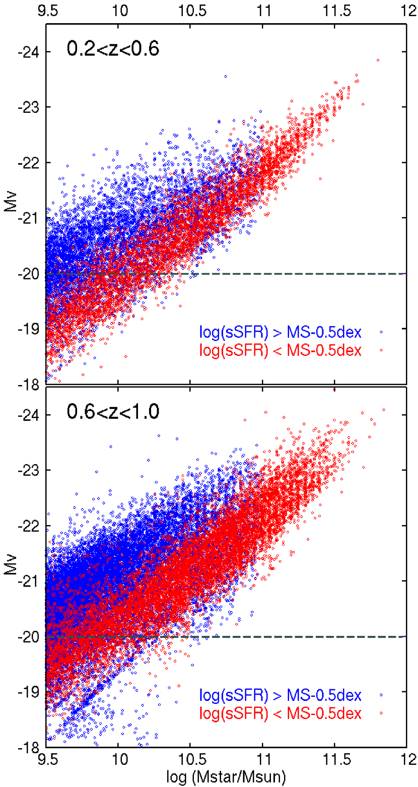
Figure 1: The rest-frame $V$-band absolute magnitude vs. stellar mass for galaxies at $0.2<z<0.6$ (top) and $0.6<z<1.0$ (bottom) in the COSMOS field. Blue symbols show star-forming galaxies with $\Delta$MS $>-0.5$ dex, and red ones represent the other galaxies with lower sSFRs of $\Delta$MS $<-0.5$ dex. The dashed line indicates the absolute magnitude limit of $M_{V}<-20$ for our sample.

The sample galaxies were detected on the Subaru/Suprime-Cam $i^{\prime}$-band data (Taniguchi et al., 2007; Capak et al., 2007), and their photometric redshifts were estimated from the multi-band photometric data from UV to MIR, which include GALEX FUV and NUV, CFHT $u*$ and $i*$, Subaru $B$, $V$, $g^{\prime}$, $r^{\prime}$, $i^{\prime}$, $z^{\prime}$, and the 12 intermediate ($IA$) bands (Taniguchi et al., 2015), VISTA $Y$, $J$, $H$, $K$, Spitzer IRAC1, 2, 3, 4 bands. The accuracy of the photometric redshift is very high with a small fraction of the catastrophic failures especially for galaxies at $z\lesssim 1.2$, where the $IA$ bands sample the Balmer break (Ilbert et al., 2013). Ilbert et al. (2013) also estimated the stellar mass and SFR by fitting the same multi-band photometry with the GALAXEV population synthesis library (Bruzual, & Charlot, 2003). In the SED fitting, they used exponentially decaying star formation histories and Calzetti extinction law (Calzetti et al., 2000), and assumed Chabrier (2003)’s Initial Mass Function.

We checked the completeness for galaxies with $M_{V}<-20$ as a function of stellar mass (Figure 1), and limited our sample to those with $M_{\rm star}>10^{9.5}M_{\odot}$ for star-forming galaxies on the main sequence (see below) and those with $M_{\rm star}>10^{10}M_{\odot}$ for the other galaxies with lower sSFRs. We note that $\sim 35$ % ($\sim$ 20 %) of galaxies with $10^{9.5}$–$10^{10}M_{\odot}$ at $0.2<z<0.6$ ($0.6<z<1.0$) for the main-sequence galaxies are missed by the absolute magnitude limit of $M_{V}<-20$, while $\sim 20$ % ($\sim$ 5–6 %) of the other galaxies with $10^{10}$–$10^{10.5}M_{\odot}$ at $0.2<z<0.6$ ($0.6<z<1.0$) are missed by the same limit. We examine how the incompleteness affects our results in Section 4.4.3. Finally, we selected total 21294 galaxies (13132 main-sequence galaxies with $M_{\rm star}>10^{9.5}M_{\odot}$ and 8162 galaxies with a lower sSFR and $M_{\rm star}>10^{10}M_{\odot}$).

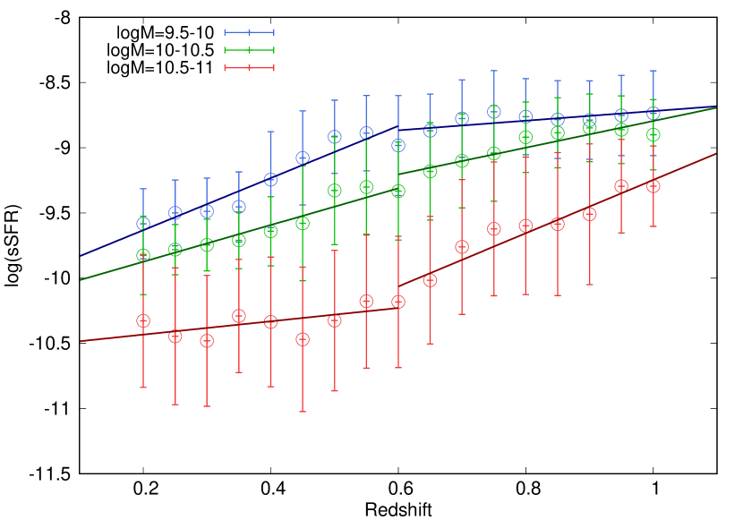
Figure 2: The clipping mean sSFRs for star-forming galaxies with different stellar masses in our sample as a function of redshift. The mean values are calculated with 2$\sigma$ clipping and additional exclusion of those with a sSFR more than 10 times lower than the mean. The different colors of symbols show galaxies with the different stellar masses. The solid lines represent the linear fitting results for those galaxies at $0.2<z<0.6$ and $0.6<z<1.0$.

Table 1: fitting results of the mean sSFR of the main sequence

redshift	stellar mass	fitted sSFR
$z=0.2$–0.6	$\log{M_{\rm star}}=9.5$–10	$\log{(sSFR)}=1.998z-10.032$
	10–10.5	$\log{(sSFR)}=1.408z-10.156$
	10.5–11	$\log{(sSFR)}=0.510z-10.535$
$z=0.6$–1.0	$\log{M_{\rm star}}=9.5$–10	$\log{(sSFR)}=0.369z-9.088$
	10–10.5	$\log{(sSFR)}=1.024z-9.819$
	10.5–11	$\log{(sSFR)}=2.043z-11.290$

In Section 4, we divide our sample by sSFR and investigate the distribution of the axial ratio as a function of sSFR. In addition to sSFR itself, we also use differences in $\log{(sSFR)}$ from the main sequence of star-forming galaxies, namely, $\Delta$MS. In order to define the main sequence, we calculated the clipping mean of sSFR for galaxies in each redshift bin with a width of $\Delta z=0.1$ (Figure 2). In the calculation, we used 2$\sigma$ clipping with additionally excluding objects with sSFR more than an order of magnitude lower than the mean. Since the sSFR of the main sequence of star-forming galaxies depends on stellar mass especially at $z\lesssim 1$ (e.g., Kajisawa et al., 2010; Ilbert et al., 2015; Popesso et al., 2019), we separately estimated the mean sSFR for galaxies with different stellar masses. Figure 2 shows the different evolutionary trends of the mean sSFR for star-forming galaxies with different masses. In order to take the evolution of the main sequence into account, we fitted the logarithm of the mean sSFR as a function of redshift with a linear line for galaxies at $0.2<z<0.6$ and $0.6<z<1.0$ separately. The fitting results are summarized in Table 1. Because there are few star-forming galaxies with $M_{\rm star}>10^{11}M_{\odot}$, we did not define the main sequence for those with $M_{\rm star}>10^{11}M_{\odot}$. In the following, we use these equations to calculate the sSFR of the main sequence and $\Delta$MS ($=\log{(sSFR)}-\log{(sSFR_{\rm MS})}$) for each object with $M_{\rm star}<10^{11}M_{\odot}$.

3 Analysis

3.1 Measurement of axial ratio

We measured apparent axial ratios of the sample galaxies on publicly available COSMOS HST/ACS $I_{\rm F814W}$-band data version 2.0 (Koekemoer et al., 2007) using the SExtractor software version 2.5.0 (Bertin, & Arnouts, 1996). The pixel scale of the data is 0.03 arcsec/pixel and the FWHM of PSF is $\sim 0.1$ arcsec. At first, we cut out a $12^{\prime\prime}\times 12^{\prime\prime}$ $I_{\rm F814W}$-band image centered on the position of each sample galaxy detected on the Subaru $i^{\prime}$-band data. We made the SEGMENTATION image for the $i^{\prime}$-band data with SExtractor, and used it to mask pixels belonging to any other $i^{\prime}$-selected objects on the $12^{\prime\prime}\times 12^{\prime\prime}$ $I_{\rm F814W}$-band image. We then ran SExtractor on the masked $I_{\rm F814W}$-band images to measure apparent axial ratios of the sample galaxies. A detection threshold of 1.3 times the local background root mean square over 12 connected pixels was used. In order to avoid the over-deblending due to the dust extinction, in particular, the dust lane in edge-on disk galaxies, we chose no deblending (DETECTED_MINCONT$=$1) and required the position of the detected object on the $I_{\rm F814W}$-band image to coincide that of the target object selected on the $i^{\prime}$-band image within 0.6 arcsec, which roughly corresponds to the FWHM of the PSF of the $i^{\prime}$-band data.

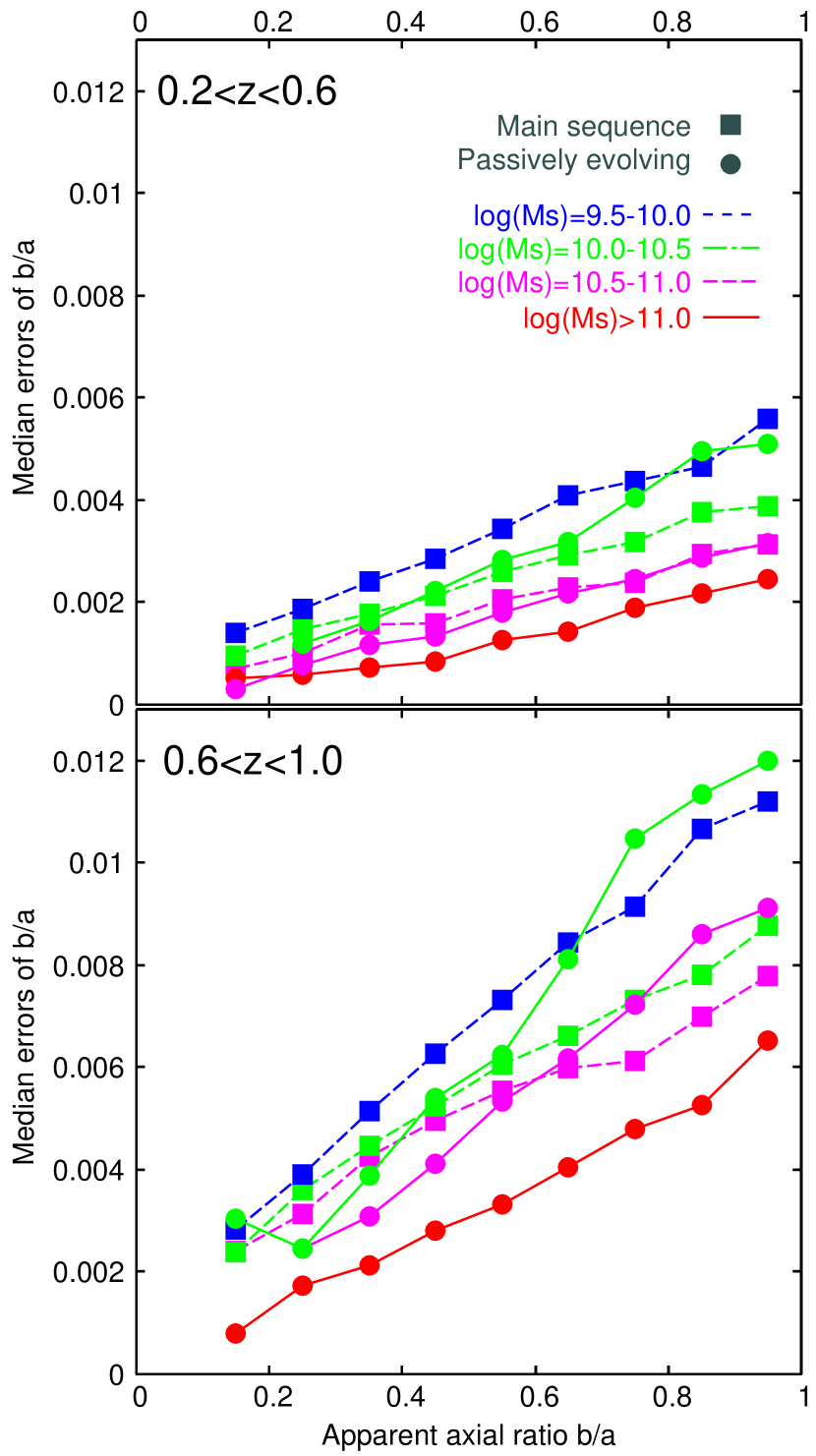
Figure 3: The median errors of the measured apparent axial ratio for our subsamples at $0.2<z<0.6$ (top) and $0.6<z<1.0$ (bottom) as a function of axial ratio. Squares show star-forming galaxies on the main sequence with $\Delta$MS $=-0.5$ – $+0.5$ dex, and circles show passively evolving galaxies with $\Delta$MS $<-1.5$ dex. The different colors of the symbols represent those galaxies with different stellar masses.

SExtractor computed the second order moments along the major and minor axes of the object as follows:

$$a^{2}=\frac{\overline{x^{2}}+\overline{y^{2}}}{2}+\sqrt{(\frac{\overline{x^{2}}-\overline{y^{2}}}{2})^{2}+\overline{xy}^{2}}$$ (1)

$$b^{2}=\frac{\overline{x^{2}}+\overline{y^{2}}}{2}-\sqrt{(\frac{\overline{x^{2}}-\overline{y^{2}}}{2})^{2}+\overline{xy}^{2}},$$ (2)

where $\overline{x^{2}}$, $\overline{y^{2}}$, and $\overline{xy}$ are the second order moments of the object in the $x$-$y$ coordinate, i.e.,

$$\overline{x^{2}}=\frac{\sum_{i\in S}I_{i}(x_{i}-\overline{x})^{2}}{\sum_{i\in S}I_{i}}$$ (3)

$$\overline{y^{2}}=\frac{\sum_{i\in S}I_{i}(y_{i}-\overline{y})^{2}}{\sum_{i\in S}I_{i}}$$ (4)

$$\overline{xy}=\frac{\sum_{i\in S}I_{i}(x_{i}-\overline{x})(y_{i}-\overline{y})}{\sum_{i\in S}I_{i}}.$$ (5)

Using the second order moments along the major and minor axes, we calculated $b/a$ as the axial ratio of the object. Since an ellipse with semi-major and minor radii of $3\times a$ and $3\times b$ usually includes most of the flux for galaxies with a normal surface brightness profile, we excluded a galaxy with $b$ smaller than 1.3 pixel (i.e., $3\times b<$ 0.1 arcsec), which is too small to reliably measure the apparent axial ratio with the spatial resolution of the HST data. There is only one object with such a small size in our sample, and it is excluded from the analysis.

While those estimated from the surface brightness fitting under the assumption of some parametric forms of the profile were used in previous studies (e.g., Padilla, & Strauss, 2008; Holden et al., 2012), the second order moments allow us to directly estimate the axial ratio without assuming the surface brightness profile of the object. On the other hand, the measured second order moments can be contributed from several components if exist for example, bulge and disk in spiral galaxies, because we didn’t carry out the decomposition of these components. It is expected that a larger and/or brighter component tends to dominate the second order moments of the object in such cases. We keep in mind these things in discussing our results.

We show examples of sample galaxies with different measured values of the axial ratio in Appendix A. Figure 3 shows median values of the statistical errors in the axial ratios as a function of axial ratio itself for the sample galaxies with different stellar masses, sSFRs, and redshifts. Although the uncertainty clearly increases with increasing axial ratio, the errors are $\delta(b/a)\sim 0.005$ at $0.2<z<0.6$ and $\sim 0.012$ at $0.6<z<1.0$ even for the least massive (faintest) galaxies in our sample. These are sufficiently small compared to a bin width of 0.1 for the axial-ratio distribution we used in this study, and the measurement errors do not significantly affect our results in the following sections.

3.2 Estimate of intrinsic 3-dimensional shape

In order to infer the intrinsic 3-dimensional shape of our sample galaxies, we fitted the distribution of the apparent axial ratio with triaxial ellipsoid models, following Ryden (2004). The shape of the triaxial model is characterized by two parameters, namely, face-on axial ratio $B/A$ and edge-on axial ratio $C/A$, where $A$, $B$, and $C$ are radii in the major, middle and minor axes ($A>B>C$). We assumed Gaussian distributions for both $B/A$ and $C/A$, and performed Monte Carlo simulations to estimate the distribution of the apparent axial ratio. We chose the Gaussian distribution for $B/A$ instead of a log-normal distribution for $\epsilon=1-B/A$ used in Ryden (2004), because the models with a Gaussian distribution for $B/A$ could reproduce the observed distributions better than those with the log-normal one, especially for star-forming (disky) galaxies. We also examined models with a Gaussian distribution for the triaxiality ($T=(A^{2}-B^{2})/(A^{2}-C^{2})$) used by Chang et al. (2013), van der Wel et al. (2014a), and Zhang et al. (2019) instead of $B/A$, and confirmed that the both models produced the similar results. We preferred those with Gaussian distributions for both $B/A$ and $C/A$ because of ease to understand the fitting results. In the simulation, we calculated an apparent axial ratio for a given combination of $B/A$ and $C/A$ assuming a random viewing angle, following Binney (1985). Thus free parameters in the fitting are the mean and dispersion of $B/A$ and $C/A$, namely, $\mu_{B/A}$, $\sigma_{B/A}$, $\mu_{C/A}$, and $\sigma_{C/A}$. For each combination of these four parameters, we carried out 100000 simulations to calculate the distribution of the apparent axial ratio. We used a bin width of 0.1 to represent the both observed and simulated distributions of the apparent axial ratio. In the simulation, we set a criterion of $\mu_{C/A}<\mu_{B/A}\leq 1$ to ensure $A>B>C$, and we calculated the apparent axial ratio by swapping $B/A$ and $C/A$ values in the case of $B/A<C/A$, which could occurs when $\mu_{C/A}$ is nearly equal to $\mu_{B/A}$ or $\sigma_{B/A}$ and/or $\sigma_{C/A}$ are relatively large. We also set a lower limit of $C/A>0.05$ to match the observed distribution of the apparent axial ratio, where there is no object with an apparent axial ratio of $b/a<0.1$ in our sample. We calculated statistical errors based on the square root of the number of sample galaxies in the bins except for bins with a very small number of objects, for which we adopted the upper and lower confidence limits given by Gehrels (1986). We simply used the grid search to find the best-fitting parameters with the minimum $\chi^{2}$ method and estimated their 68% confidence ranges with the $\Delta\chi^{2}$ method. In the fitting procedures, $\mu_{B/A}$ and $\mu_{C/A}$ range from 0.05 to 1 with a step of 0.005, and $\sigma_{C/A}$ ranges from 0.01 to 0.5 with a step of 0.01. We used three step widths for $\sigma_{B/A}$, namely, 0.01 at $0.01<\sigma_{B/A}<0.5$, 0.02 at $0.5<\sigma_{B/A}<0.8$, and 0.04 at $0.8<\sigma_{B/A}<1.0$. We present the fitting results for subsamples used in this study in Appendix B and Table 2. The best-fit models are consistent with the observed distributions within the errors for all the subsamples.

4 Results

4.1 Dependence of axial ratio & 3-D shape on sSFR

Figure 4: The distribution of the apparent axial ratio for subsamples at $0.2<z<0.6$ as a function of sSFR and stellar mass. The sSFR decreases from top to bottom row, and the stellar mass increases from left to right column. The error bars are based on the square root of the number of objects in the bin except for cases with a very small number of objects (see text). The distribution for star-forming galaxies on the main sequence with $\Delta$MS $=-0.5$ – $+0.5$ dex in the same mass range is also shown for reference, although that of those galaxies with $\log{(sSFR)}>-12$ are plotted for reference in the $M_{\rm star}>10^{11}M_{\odot}$ bins. The total number of objects in the subsample is also shown in each panel.

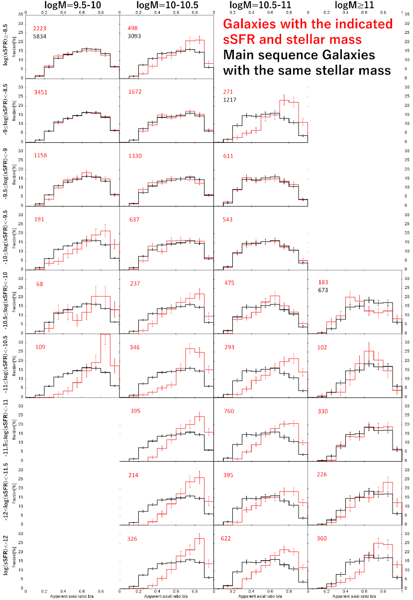
Figure 5: Same as Figure 4, but for galaxies at $0.6<z<1.0$. In the $M_{\rm star}>10^{11}M_{\odot}$ bins, that of those galaxies with $\log{(sSFR)}>-11.5$ is plotted for reference.

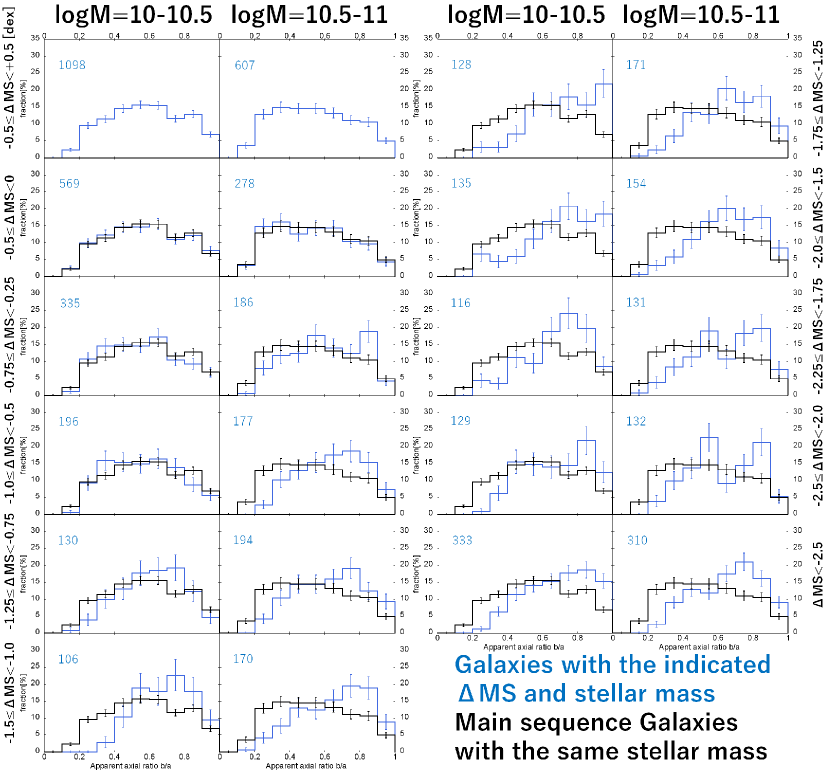
Figure 6: The distribution of the apparent axial ratio for subsamples at $0.2<z<0.6$ as a function of $\Delta$MS and stellar mass. The $\Delta$MS decreases from top to bottom row, and the panels in the left (right) column show galaxies with $M_{\rm star}=10^{10}$–$10^{10.5}M_{\odot}$ ($10^{10.5}$–$10^{11}M_{\odot}$). The distribution for the main-sequence galaxies with $\Delta$MS $=-0.5$ – $+0.5$ dex in the same mass range is also shown for reference. The total number of objects in the subsample is also shown in each panel.

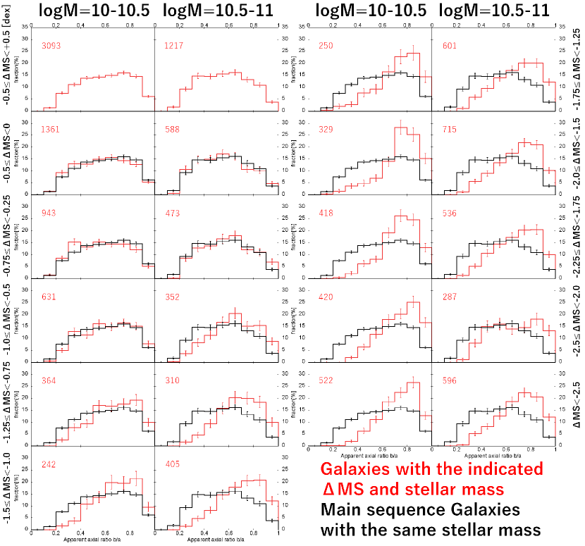
Figure 7: Same as Figure 6, but for galaxies at $0.6<z<1.0$.

In order to investigate the 3-dimensional shape of galaxies as a function of redshift, stellar mass, and sSFR, we divided the sample galaxies into subsamples with different properties and derived their distribution of the axial ratio separately. We basically divided by redshift into those at $0.2<z<0.6$ and $0.6<z<1.0$ to study the evolution, and by stellar mass into those with $M_{\rm star}=10^{9.5}$–$10^{10}M_{\odot}$, $10^{10}$–$10^{10.5}M_{\odot}$, $10^{10.5}$–$10^{11}M_{\odot}$, and $M_{\rm star}>10^{11}M_{\odot}$ to investigate the mass dependence. Figures 4 and 5 show the distribution of the axial ratio as a function of sSFR for galaxies at $0.2<z<0.6$ and $0.6<z<1.0$, respectively. We plot only those for the subsamples with sufficient number of objects ($n>50$) to ensure the statistical accuracy. For $M_{\rm star}=10^{9.5}$–$10^{10}M_{\odot}$, galaxies with a relatively low sSFR are missed from our sample due to the incompleteness by the criterion of $M_{V}<-20$ as mentioned in Section 2. On the other hand, the number of massive star-forming galaxies with $M_{\rm star}\gtrsim 10^{11}M_{\odot}$ is intrinsically small, and the results for these galaxies are also not shown in the figures.

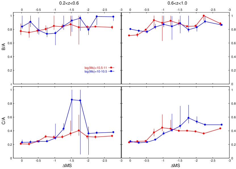
Figure 8: The best-fit mean values of the intrinsic face-on axial ratio $\mu_{B/A}$ (top panels) and edge-on axial ratio $\mu_{C/A}$ (bottom panels) as a function of $\Delta$MS for galaxies at $0.2<z<0.6$ (left) and $0.6<z<1.0$ (right). Blue symbols show galaxies with $M_{\rm star}=10^{10}$–$10^{10.5}M_{\odot}$, and red symbols show those with $10^{10.5}$–$10^{11}M_{\odot}$. The error bars represent the 68% confidence ranges of the $\mu_{B/A}$ and $\mu_{C/A}$.

In Figures 4 and 5, one can see the axial-ratio distribution changes with decreasing sSFR for most of the redshift and stellar mass bins. We also plot the distribution for star-forming galaxies on the main sequence, i.e., those with $\Delta$MS $=-0.5$ – $+0.5$ dex in the same redshift and stellar mass bin for reference. For those with $M_{\rm star}>10^{11}M_{\odot}$, we could not define the main sequence as mentioned in Section 2 and plot that of galaxies with $sSFR>10^{-12}$ yr^-1 at $0.2<z<0.6$ and those with $sSFR>10^{-11.5}$ yr${}^{{}^{-}1}$ at $0.6<z<1.0$ in the same mass range for reference. The distribution for star-forming galaxies at a relatively high sSFR tends to be flat with a plateau over $b/a=$ 0.3 – 0.9. On the other hand, the fraction of galaxies with $b/a<0.5$ decreases with decreasing sSFR, and the distributions at low sSFRs have a peak around $b/a\sim$ 0.8 – 0.9. As shown in previous studies, the flat distribution indicates a relatively flat disk 3-dimensional shape, while that with a peak around $b/a\sim$ 0.8 – 0.9 is expected for more thick spheroidal shape. Thus Figures 4 and 5 suggest that star-forming galaxies except for those with a extremely high sSFR are basically disk-dominated galaxies and passively evolving galaxies with a low sSFR have spheroidal morphology, which is consistent with the results in many previous studies at $z<1$ mentioned in Section 1.

The sSFR at which the transition from the flat distribution to that with a peak around $b/a\sim$ 0.8 – 0.9 occurs seems to depend on both redshift and stellar mass. The distributions for galaxies with $M_{\rm star}=10^{10}$–$10^{10.5}M_{\odot}$ and $10^{10.5}$–$10^{11}M_{\odot}$ at $0.2<z<0.6$ significantly change around $sSFR\sim 10^{-11}$ yr^-1 and $\sim 10^{-11.5}$ yr^-1, respectively. On the other hand, those for galaxies in the same mass ranges at $0.6<z<1.0$ change around $sSFR\sim 10^{-10.5}$ yr^-1 and $\sim 10^{-11}$ yr^-1, respectively. The transition sSFR is higher for less massive galaxies at higher redshift. In order to investigate the relationship between the transition sSFR and the main sequence of star-forming galaxies, we divided our sample by $\Delta$MS defined in Section 2 instead of sSFR itself and plot the distribution of the apparent axial ratio as a function of $\Delta$MS in Figures 6 and 7 for galaxies at $0.2<z<0.6$ and $0.6<z<1.0$, respectively. We defined those with $-0.5<\Delta$MS $<0.5$ as “main-sequence” galaxies and plot the distribution of these galaxies in each panel for reference. The other subsamples have a bin width of 0.5 dex in $\Delta$MS that is offsetted by 0.25 dex from the next ones. In Figures 6 and 7, the distribution for the main-sequence galaxies is flat, and the transition of the distribution occurs at $\Delta$MS $\sim-1$ dex for the both redshift ranges. The distribution of galaxies with $M_{\rm star}=10^{10.5}$–$10^{11}M_{\odot}$ changes at $\Delta$MS $\sim-0.75$ dex, which is slightly higher than that of galaxies with $10^{10}$–$10^{10.5}M_{\odot}$ in the both redshift bins.

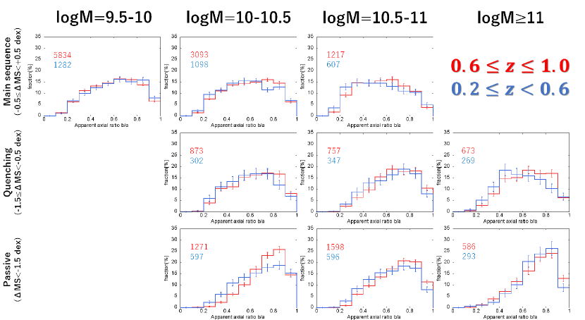
Figure 9: The evolution of the distribution of the apparent axial ratio as a function of $\Delta$MS and stellar mass. Top, middle, and bottom panels show the main-sequence galaxies with $\Delta$MS $=-0.5$ – $+0.5$ dex, quenching galaxies with $\Delta$MS $=-1.5$ – $-0.5$ dex, and passively evolving galaxies with $\Delta$MS $<-1.5$ dex, respectively. The stellar mass increases from left to right panels. Blue lines show those galaxies at $0.2<z<0.6$ and red lines show those at $0.6<z<1.0$. Note that massive galaxies with $M_{\rm star}>10^{11}M_{\odot}$ are divided into quenching and passively evolving subsamples at a sSFR of $10^{-12}$ and $10^{-11.5}$ yr^-1 for those at $0.2<z<0.6$ and $0.6<z<1.0$, respectively, where the change of the axial-ratio distribution occurs (see text).

Using the Monte Carlo simulation described in Section 3.2, we then fitted the distribution of each subsample in Figures 6 and 7 with the triaxial ellipsoid models to estimate the intrinsic 3-dimensional shape. The comparisons with the best-fit models and the observed distributions for the subsamples are presented in Appendix B. We show the estimated mean values of the intrinsic face-on axial ratio and edge-on axial ratio, namely, $\mu_{B/A}$ and $\mu_{C/A}$ as a function of $\Delta$MS in Figure 8. The face-on axial ratio $B/A$ seems to increase with decreasing $\Delta$MS from $B/A\sim$ 0.7 – 0.85 at $\Delta$MS $\sim 0$ to $B/A\sim$ 0.8 – 0.95 at $\Delta$MS $\sim-2.5$ in the all redshift and stellar mass bins we investigated, but we cannot conclude it because the uncertainty in the estimates of $B/A$ is large. The $B/A$ of galaxies with $M_{\rm star}=10^{10}$–$10^{10.5}M_{\odot}$ may be systematically higher than those with $10^{10.5}$–$10^{11}M_{\odot}$ at $0.2<z<0.6$ although the uncertainty is large, while those with the different mass ranges are consistent with each other within uncertainty at $0.6<z<1.0$.

On the other hand, the edge-on axial ratio $C/A$ (i.e., thickness) clearly increases with decreasing $\Delta$MS from $C/A\sim$ 0.2 – 0.25 at $\Delta$MS $\sim 0$ to $C/A\sim$ 0.3 – 0.5 at $\Delta$MS $\lesssim-1.5$, although the uncertainty in some of bins at $-2<\Delta$MS $<-1$ is relatively large due to a small number of objects especially for less massive and lower redshift bins. The transition from $C/A\sim$ 0.2 – 0.25 to $\sim$ 0.3 – 0.5 occurs around $\Delta$MS $\sim-1$ dex in the all redshift and mass bins, which is consistent with the results in Figures 6 and 7. One can also see the $C/A$ of galaxies with $M_{\rm star}=10^{10}$–$10^{10.5}M_{\odot}$ changes at a slightly higher $\Delta$MS of $\sim-0.75$ dex than that of galaxies with $10^{10.5}$–$10^{11}M_{\odot}$ in the both redshift ranges.

We also note that the distributions of the apparent axial ratio of galaxies with $M_{\rm star}=10^{10}$–$10^{10.5}M_{\odot}$ and $\Delta$MS $\sim-2.0$ – $-1.5$ at $0.2<z<0.6$ are fitted with models with a nearly spherical shape of $B/A\sim C/A\sim 1$ and their uncertainty of $\mu_{C/A}$ is extremely large. The small numbers of objects in these bins ($n\sim 130$) make the statistical uncertainty of the distribution relatively large, and the constraints on the intrinsic axial ratios are weak. Furthermore, while the distributions have a broad peak around $b/a\sim 0.8$ – 1.0, there are also a non-negligible fraction of galaxies with $b/a=0.2$ – 0.3. Such distributions cannot be explained by the models with a narrow range of $C/A$, and only the models with a relatively large $\sigma_{C/A}$ enable to reproduce these distributions (see Appendix C for details). In such cases with a large $\sigma_{C/A}$, there are models with various $\mu_{C/A}$ values allowed by the observed distribution, which leads to the very large uncertainty of $\mu_{C/A}$ for these galaxies. With the small sizes of these subsamples, we cannot conclude whether the non-negligible fractions of galaxies with $b/a=0.2$ – 0.3 are caused by the statistical fluctuation or not.

4.2 Evolution of axial ratio & 3-D shape

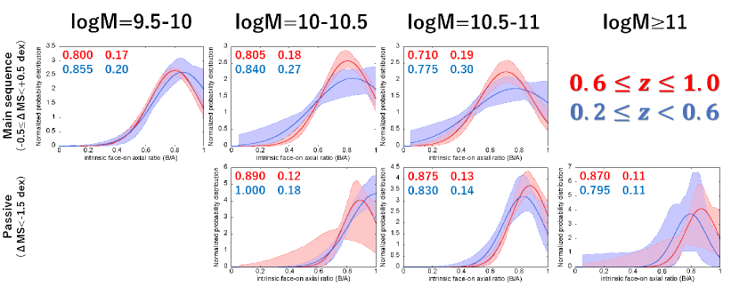
Figure 10: The probability distribution of the intrinsic face-on axial ratio $B/A$ calculated from the best-fit $\mu_{B/A}$ and $\sigma_{B/A}$ as a function of stellar mass for the main sequence (top) and passively evolving (bottom) subsamples. The stellar mass increases from left to right panels. Blue lines show those galaxies at $0.2<z<0.6$ and red lines show those at $0.6<z<1.0$. The shaded regions represent the 68% confidence ranges calculated with the $\Delta\chi^{2}$ method. The best-fit $\mu_{B/A}$ and $\sigma_{B/A}$ values are also shown in each panel.

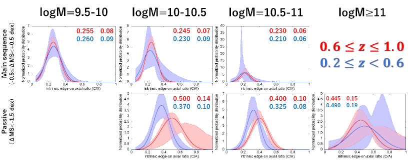
Figure 11: Same as Figure 10, but for the intrinsic edge-on axial ratio $C/A$ calculated from the best-fit $\mu_{C/A}$ and $\sigma_{C/A}$.

Table 2: the best-fit parameters of the triaxial ellipsoid models for the subsamples

stellar mass	$\Delta$MS	$\mu_{B/A}$	$\sigma_{B/A}$	$\mu_{C/A}$	$\sigma_{C/A}$	$\chi^{2}_{\rm min}$
$z=0.2$–0.6
$\log{M_{\rm star}}=9.5$–10	$\Delta$MS $=-0.5$ – $+0.5$	$0.855^{+0.095}_{-0.055}$	$0.20^{+0.07}_{-0.05}$	$0.265^{+0.025}_{-0.020}$	$0.09^{+0.04}_{-0.03}$	5.66
$\log{M_{\rm star}}=10$–10.5	$\Delta$MS $=-0.5$ – $+0.5$	$0.840^{+0.160}_{-0.070}$	$0.27^{+0.25}_{-0.07}$	$0.230^{+0.080}_{-0.025}$	$0.09^{+0.11}_{-0.04}$	10.7
	$\Delta$MS $=-1.5$ – $-0.5$	$0.780^{+0.220}_{-0.055}$	$0.17^{+0.18}_{-0.05}$	$0.275^{+0.065}_{-0.035}$	$0.06^{+0.05}_{-0.05}$	1.27
	$\Delta$MS $<-1.5$	$1.000^{+0.000}_{-0.110}$	$0.18^{+0.03}_{-0.07}$	$0.370^{+0.035}_{-0.030}$	$0.10^{+0.04}_{-0.02}$	1.61
$\log{M_{\rm star}}=10.5$–11	$\Delta$MS $=-0.5$ – $+0.5$	$0.775^{+0.225}_{-0.100}$	$0.30^{+0.34}_{-0.09}$	$0.210^{+0.06}_{-0.03}$	$0.06^{+0.08}_{-0.05}$	1.07
	$\Delta$MS $=-1.5$ – $-0.5$	$0.830^{+0.170}_{-0.050}$	$0.14^{+0.13}_{-0.05}$	$0.315^{+0.040}_{-0.035}$	$0.08^{+0.04}_{-0.03}$	0.263
	$\Delta$MS $<-1.5$	$0.830^{+0.115}_{-0.035}$	$0.14^{+0.10}_{-0.04}$	$0.325^{+0.035}_{-0.020}$	$0.08^{+0.02}_{-0.02}$	1.45
$\log{M_{\rm star}}>11$	$\log{(sSFR)}>-12.0$	$0.835^{+0.165}_{-0.195}$	$0.33^{+0.67}_{-0.17}$	$0.335^{+0.125}_{-0.075}$	$0.10^{+0.07}_{-0.05}$	0.847
	$\log{(sSFR)}<-12.0$	$0.795^{+0.205}_{-0.130}$	$0.11^{+0.89}_{-0.05}$	$0.490^{+0.245}_{-0.055}$	$0.19^{+0.31}_{-0.11}$	3.19
$z=0.6$–1.0
$\log{M_{\rm star}}=9.5$–10	$\Delta$MS $=-0.5$ – $+0.5$	$0.800^{+0.015}_{-0.020}$	$0.17^{+0.02}_{-0.01}$	$0.255^{+0.010}_{-0.010}$	$0.08^{+0.01}_{-0.01}$	2.02
10–10.5	$\Delta$MS $=-0.5$ – $+0.5$	$0.805^{+0.020}_{-0.025}$	$0.18^{+0.03}_{-0.03}$	$0.245^{+0.010}_{-0.010}$	$0.07^{+0.01}_{-0.01}$	11.4
	$\Delta$MS $=-1.5$ – $-0.5$	$0.840^{+0.075}_{-0.045}$	$0.15^{+0.07}_{-0.03}$	$0.295^{+0.030}_{-0.015}$	$0.07^{+0.03}_{-0.02}$	4.42
	$\Delta$MS$<-1.5$	$0.890^{+0.110}_{-0.170}$	$0.12^{+0.26}_{-0.04}$	$0.500^{+0.245}_{-0.025}$	$0.14^{+0.15}_{-0.02}$	1.48
$\log{M_{\rm star}}=10.5$–11	$\Delta$MS$=-0.5$ – $+0.5$	$0.710^{+0.040}_{-0.020}$	$0.19^{+0.05}_{-0.03}$	$0.230^{+0.020}_{-0.020}$	$0.06^{+0.02}_{-0.02}$	3.06
	$\Delta$MS $=-1.5$ – $-0.5$	$0.915^{+0.085}_{-0.090}$	$0.20^{+0.14}_{-0.08}$	$0.385^{+0.080}_{-0.035}$	$0.12^{+0.05}_{-0.03}$	5.92
	$\Delta$MS $<-1.5$	$0.875^{+0.030}_{-0.030}$	$0.13^{+0.03}_{-0.03}$	$0.400^{+0.015}_{-0.020}$	$0.10^{+0.01}_{-0.02}$	5.06
$\log{M_{\rm star}}>11$	$\log{(sSFR)}>-11.5$	$0.810^{+0.060}_{-0.050}$	$0.16^{+0.09}_{-0.05}$	$0.335^{+0.035}_{-0.030}$	$0.09^{+0.04}_{-0.02}$	4.56
	$\log{(sSFR)}<-11.5$	$0.870^{+0.130}_{-0.175}$	$0.11^{+0.32}_{-0.04}$	$0.445^{+0.285}_{-0.035}$	$0.15^{+0.18}_{-0.04}$	0.490

In order to investigate the evolution of the intrinsic shape of star-forming and passively evolving galaxies with high statistical accuracy, we here divided our sample by $\Delta$MS into three subsamples, namely, star-forming main-sequence galaxies with $-0.5<\Delta$MS $<0.5$, quenching galaxies with $-1.5<\Delta$MS $<-0.5$, and passively evolving galaxies with $\Delta$MS $<-1.5$. We chose these criteria in $\Delta$MS taking account of the $\Delta$MS dependence of the axial-ratio distribution and its transition found in the previous section. The main-sequence galaxies have the relatively flat distribution of the apparent axial ratio, which suggests low-$C/A$ disky morphology, while passively evolving galaxies show higher-$C/A$ and thick spheroidal morphology. Quenching galaxies are defined as that between these two populations. For galaxies with $M_{\rm star}>10^{11}M_{\odot}$, we cannot define the main sequence and therefore used constant $sSFR$ values as criteria. We divided these massive galaxies into quenching and passively evolving subsamples at $sSFR=10^{-12}$ and $10^{-11.5}$ yr^-1 for those at $0.2<z<0.6$ and $0.6<z<1.0$, respectively. We also set these criteria for massive galaxies taking account of the transition of the axial-ratio distribution.

In Figure 9, we compare the distributions of the apparent axial ratio for galaxies at $0.2<z<0.6$ and $0.6<z<1.0$ in each stellar mass and $\Delta$MS bin. Those of the main-sequence galaxies in the two redshift bins are consistent with each other within uncertainty in the all mass ranges, although the fraction of galaxies with $b/a\sim$ 0.7 – 0.8 is marginally higher at $0.6<z<1.0$ for galaxies with $M_{\rm star}=10^{10}$–$10^{11}M_{\odot}$. These galaxies basically show the flat distribution. On the other hand, passively evolving galaxies with $M_{\rm star}<10^{11}M_{\odot}$ show a significant evolution. Those galaxies at $0.2<z<0.6$ have the flatter distribution with higher fraction of objects with $b/a<0.5$ and lower peak around $b/a\sim$ 0.8 – 0.9 than those at $0.6<z<1.0$. The evolution seems to be stronger for passively evolving galaxies with $M_{\rm star}=10^{10}$–$10^{10.5}M_{\odot}$ than those with $10^{10.5}$–$10^{11}M_{\odot}$. In contrast to these galaxies with $M_{\rm star}<10^{11}M_{\odot}$, massive passively evolving galaxies with $M_{\rm star}>10^{11}M_{\odot}$ show no significant evolution, although the uncertainty is relatively large due to a small number of these massive galaxies. These massive galaxies have more peaky distribution skewed toward high $b/a$ value than less massive ones with $10^{10.5}$–$10^{11}M_{\odot}$ in the both redshift ranges.

Quenching galaxies show marginal differences between those at $0.2<z<0.6$ and $0.6<z<1.0$, although the uncertainty is large. The subsamples at $0.2<z<0.6$ tend to have the flatter distribution or that skewed toward lower $b/a$ value, but this could depend on the choice of the criteria in $\Delta$MS for these galaxies. On the other hand, the evolutionary trends of the main-sequence and passively evolving populations mentioned above are not changed by the choice of the criteria.

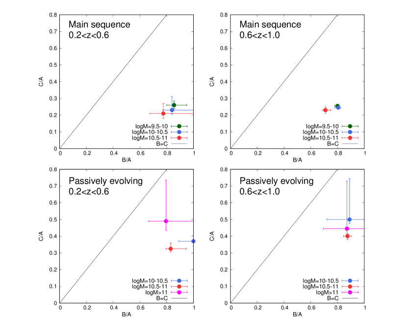
Figure 12: The best-fit values of the mean intrinsic face-on axial ratio $\mu_{B/A}$ and edge-on axial ratio $\mu_{C/A}$ for the main-sequence galaxies (top panels) and passively evolving galaxies (bottom panels) at $0.2<z<0.6$ (left) and $0.6<z<1.0$ (right). The different colors show galaxies with different stellar masses. The error bars represent the 68% confidence ranges of the $\mu_{B/A}$ and $\mu_{C/A}$. The diagonal line indicates the criterion of $B/A>C/A$ set from the definition of $A>B>C$.

We estimated the intrinsic 3-dimensional shape from the distribution of the apparent axial ratio for the main sequence and passively evolving populations with the Monte Carlo simulations, and show the results for the face-on axial ratio $B/A$ and edge-on axial ratio $C/A$ in Figures 10 and 11, respectively. In the figures, we plot the probability distributions of $B/A$ and $C/A$ and their uncertainty estimated from the best-fit parameters and their errors, and compare those for galaxies at $0.2<z<0.6$ and $0.6<z<1.0$. Note that these are not the likelihood functions of $\mu_{B/A}$ and $\mu_{C/A}$, but the Gaussian probability distributions calculated from the best-fit values of $\mu_{B/A}$, $\sigma_{B/A}$, $\mu_{C/A}$, and $\sigma_{C/A}$, and their confidence ranges. Since each Gaussian distribution is normalized so that the integration over $B/A$ or $C/A$ becomes unity, the confidence range of the probability would be high if a relatively small value of $\sigma_{B/A}$ or $\sigma_{C/A}$, which corresponds to a narrow Gaussian distribution, is allowed for a certain value of $\mu_{B/A}$ or $\mu_{C/A}$. The fitting results are also summarized in Table 2.

The main-sequence galaxies show no evolution in the edge-on axial ratio $C/A$, while the face-on axial ratio $B/A$ of these galaxies show marginal changes at $M_{\rm star}>10^{10}M_{\odot}$. The mean values of $B/A$ of those galaxies with $M_{\rm star}=10^{10}$–$10^{10.5}M_{\odot}$ ($10^{10.5}$–$10^{11}M_{\odot}$) evolve from $\mu_{B/A}=0.805$ (0.710) at $0.6<z<1.0$ to $\mu_{B/A}=0.840$ (0.775) at $0.2<z<0.6$, while $\sigma_{B/A}$ also increases with time. On the other hand, passively evolving galaxies with $M_{\rm star}<10^{11}M_{\odot}$ show a significant evolution in the edge-on axial ratio $C/A$. The mean values of $C/A$ of passively evolving galaxies with $M_{\rm star}=10^{10}$–$10^{10.5}M_{\odot}$ ($10^{10.5}$–$10^{11}M_{\odot}$) decreases with time from $\mu_{C/A}=0.500$ (0.400) at $0.6<z<1.0$ to $\mu_{C/A}=0.370$ (0.325) at $0.2<z<0.6$. Passively evolving galaxies with $M_{\rm star}>10^{11}M_{\odot}$ have relatively high $C/A$ values but show no significant evolution in both $B/A$ and $C/A$. We summarize the mean values of $B/A$ and $C/A$ for star-forming and passively evolving galaxies in Figure 12. It is seen that $C/A$ of passively evolving galaxies with $M_{\rm star}<10^{11}M_{\odot}$ decreases with time, while main-sequence galaxies show no significant evolution but only marginal changes in $B/A$.

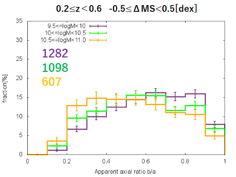
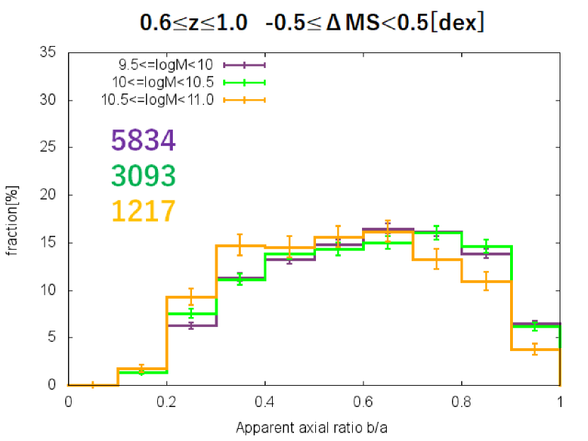
Figure 13: The mass dependence of the distribution of the apparent axial ratio for the main-sequence galaxies at $0.2<z<0.6$ (left) and $0.6<z<1.0$ (right). The different colors of the lines show galaxies with different stellar masses. The total numbers of objects in the subsamples are also shown in each panel.

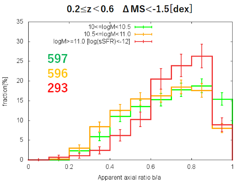
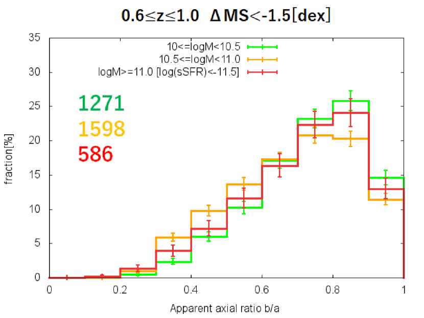
Figure 14: Same as Figure 13, but for the passively evolving galaxies.

4.3 Mass dependence of axial ratio & 3-D shape

In Figure 13, we compare the distributions of the apparent axial ratio for the main-sequence subsamples with different stellar mass ranges to investigate the mass dependence of the 3-dimensional shape of star-forming galaxies. While the distributions for all the main-sequence subsamples are relatively flat over $b/a\sim$ 0.2 – 1.0, more massive galaxies tend to show lower values of $b/a$ in the both redshift ranges. More massive main-sequence galaxies have a higher fraction of objects with $b/a<0.5$ and a lower fraction of those with $b/a>0.8$ than less massive ones. The mass dependence of the distribution in the main-sequence galaxies reflects mass-dependent edge-on axial ratio $C/A$ (thickness) of these galaxies seen in Figure 12. Main-sequence galaxies with $M_{\rm star}=10^{9.5}$–$10^{10}M_{\odot}$, $10^{10}$–$10^{10.5}M_{\odot}$, and $10^{10.5}$–$10^{11}M_{\odot}$ at $0.2<z<0.6$ ($0.6<z<1.0$) have the best-fit mean values of the edge-on axial ratio $\mu_{C/A}=$ 0.265, 0.230, and 0.210 (0.255, 0.245, and 0.230), respectively. The thickness of star-forming galaxies on the main sequence decreases with stellar mass in the both redshift ranges, although the uncertainty in these estimated values is not negligible, especially for more massive galaxies at lower redshift. It is also noted that those galaxies with $M_{\rm star}=10^{10.5}$–$10^{11}M_{\odot}$ show lower values of the face-on axial ratio $B/A$ than those less massive galaxies with $M_{\rm star}<10^{10.5}M_{\odot}$ in the both redshift ranges. The difference in $B/A$ may reflect the contribution from the bulge or bar structure, since more massive star-forming galaxies tend to show the high bulge fraction and/or strong bar (e.g., Bluck et al., 2019; Cervantes Sodi, 2017).

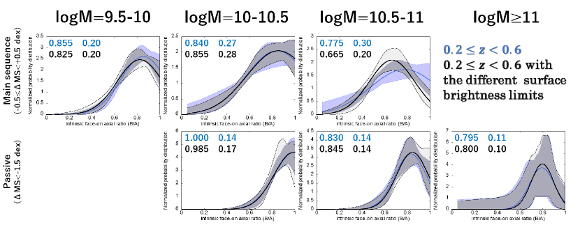
Figure 15: Same as Figure 10, but for galaxies at $0.2<z<0.6$ with the different surface brightness limits in the measurements of the apparent axial ratio. While blue lines show the results in the original analysis, the black lines show those with the two times brighter surface brightness limit.

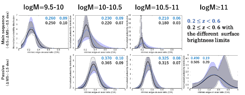
Figure 16: Same as Figure 15, but for the intrinsic edge-on axial ratio $C/A$.

On the other hand, passively evolving galaxies show more complex dependence of the axial-ratio distribution on stellar mass. Figure 14 shows the distribution of the apparent axial ratio for passively evolving galaxies with the different mass ranges in each redshift range. In the both redshift ranges, those galaxies with $M_{\rm star}=10^{10.5}$–$10^{11}M_{\odot}$ show more flatter distribution and a higher fraction of objects with $b/a<0.5$ than the subsamples with $M_{\rm star}>10^{11}M_{\odot}$ and $M_{\rm star}=10^{10}$–$10^{10.5}M_{\odot}$. The distribution of those with $M_{\rm star}=10^{10}$–$10^{10.5}M_{\odot}$ is clearly flatter than massive galaxies with $M_{\rm star}>10^{11}M_{\odot}$ at $0.2<z<0.6$, while the distribution of those low-mass galaxies is similar with that of massive galaxies at $0.6<z<1.0$. In Figure 12, passively evolving galaxies with $M_{\rm star}=10^{10.5}$–$10^{11}M_{\odot}$ similarly show lower $\mu_{C/A}$ values than those with $M_{\rm star}>10^{11}M_{\odot}$ and $M_{\rm star}=10^{10}$–$10^{10.5}M_{\odot}$ in the both redshift ranges. The $\mu_{C/A}$ value of those with $10^{10}$–$10^{10.5}M_{\odot}$ is lower than the most massive galaxies at $0.2<z<0.6$, while they show the similar $\mu_{C/A}$ values at $0.6<z<1.0$. As seen in the previous section, the thickness of those with $10^{10}$–$10^{10.5}M_{\odot}$ and $10^{10.5}$–$10^{11}M_{\odot}$ clearly decreases with time from $\mu_{C/A}=0.500$ and 0.400 at $0.6<z<1.0$ to 0.370 and 0.325 at $0.2<z<0.6$, respectively. Although the evolution in the thickness is stronger for lower mass galaxies, the $\mu_{C/A}$ value of those with $10^{10}$–$10^{10.5}M_{\odot}$ is still higher than those with $10^{10.5}$–$10^{11}M_{\odot}$ even at $0.2<z<0.6$. The most massive galaxies show no significant evolution in their intrinsic shape and they have relatively high $\mu_{C/A}$ values of 0.45 – 0.49.

4.4 possible biases

We here examine possible biases that could affect the results described in the previous sections, namely, the cosmological surface brightness dimming, morphological K-correction, incompleteness by the absolute magnitude limit, environmental effect, and size dependence of the axial-ratio distribution.

4.4.1 Cosmological surface brightness dimming

Table 3: the best-fit parameters for galaxies at $0.2<z<0.6$ with the two times brighter surface brightness limit

stellar mass	$\Delta$MS	$\mu_{B/A}$	$\sigma_{B/A}$	$\mu_{C/A}$	$\sigma_{C/A}$	$\chi^{2}_{\rm min}$
$z=0.2$–0.6
$\log{M_{\rm star}}=9.5$–10	$\Delta$MS $=-0.5$ – $+0.5$	$0.825^{+0.135}_{-0.045}$	$0.20^{+0.10}_{-0.05}$	$0.250^{+0.025}_{-0.025}$	$0.10^{+0.05}_{-0.03}$	6.55
$\log{M_{\rm star}}=10$–10.5	$\Delta$MS $=-0.5$ – $+0.5$	$0.855^{+0.145}_{-0.085}$	$0.28^{+0.17}_{-0.07}$	$0.220^{+0.050}_{-0.020}$	$0.07^{+0.09}_{-0.02}$	5.54
	$\Delta$MS $=-1.5$ – $-0.5$	$0.780^{+0.095}_{-0.040}$	$0.14^{+0.09}_{-0.04}$	$0.255^{+0.030}_{-0.030}$	$0.04^{+0.03}_{-0.03}$	2.09
	$\Delta$MS $<-1.5$	$0.985^{+0.015}_{-0.115}$	$0.17^{+0.04}_{-0.09}$	$0.365^{+0.030}_{-0.030}$	$0.09^{+0.03}_{-0.02}$	1.11
$\log{M_{\rm star}}=10.5$–11	$\Delta$MS $=-0.5$ – $+0.5$	$0.665^{+0.050}_{-0.030}$	$0.20^{+0.07}_{-0.04}$	$0.180^{+0.030}_{-0.020}$	$0.03^{+0.06}_{-0.02}$	3.54
	$\Delta$MS $=-1.5$ – $-0.5$	$0.840^{+0.160}_{-0.040}$	$0.14^{+0.16}_{-0.05}$	$0.310^{+0.050}_{-0.035}$	$0.08^{+0.04}_{-0.02}$	2.75
	$\Delta$MS $<-1.5$	$0.845^{+0.155}_{-0.040}$	$0.14^{+0.12}_{-0.04}$	$0.315^{+0.035}_{-0.020}$	$0.07^{+0.03}_{-0.01}$	1.61
$\log{M_{\rm star}}>11$	$\log{(sSFR)}>-12.0$	$0.755^{+0.245}_{-0.285}$	$0.26^{+0.74}_{-0.12}$	$0.330^{+0.185}_{-0.090}$	$0.11^{+0.39}_{-0.06}$	2.39
	$\log{(sSFR)}<-12.0$	$0.800^{+0.200}_{-0.110}$	$0.10^{+0.78}_{-0.04}$	$0.505^{+0.245}_{-0.060}$	$0.20^{+0.30}_{-0.12}$	0.701

As described in Section 3.1, we used the surface brightness threshold of 1.3 times the local background root mean square in the measurements of the apparent axial ratio on the $I_{\rm F814W}$-band data. Since the surface brightness of objects decreases with increasing redshift by a factor of $(1+z)^{4}$ ($(1+z)^{3}$ in AB mag/arcsec²) due to the cosmological expansion, the constant isophotal threshold in the measurements corresponds to the brighter intrinsic surface brightness limit for galaxies at higher redshifts. Thus the apparent axial ratio of a galaxy at higher redshift tends to be measured in a brighter part of the object. This bias could affect our results about the evolution of the axial-ratio distribution in the previous sections.

In order to check the effects of the cosmological surface brightness dimming, we re-analyzed the sample galaxies at $0.2<z<0.6$ with a surface brightness threshold two times brighter than that in the original analysis. We chose the factor of two considering the average dimming factor ratio of $(1+0.8)^{3}/(1+0.4)^{3}$ between our subsamples at $0.2<z<0.6$ and $0.6<z<1.0$. Using the measurements with the brighter surface brightness threshold, we carried out the same analyses to calculate the distribution of the apparent axial ratio as a function of stellar mass and $\Delta$MS and estimate the 3-dimensional shape with the Monte Carlo simulations. In Figures 15 and 16, we show the results of the intrinsic face-on axial ratio $B/A$ and edge-on axial ratio $C/A$ and compare them with those in the original analysis. The fitting results are also summarized in Table 3. The all results with the brighter threshold are consistent with the original ones within the errors. Although the edge-on axial ratio $C/A$ tends to be lower values by $\sim 0.01$ in the results with the brighter threshold, the differences are small and within the uncertainty. We conclude that the cosmological surface brightness dimming does not significantly affect our results. We also note that the effects of the brighter threshold on the results do not depend on stellar mass. Thus, it is not the case that low-mass (faint) galaxies are preferentially affected by the surface brightness limit. For example, the mass dependence of the $C/A$ for the main-sequence galaxies, i.e., thicker shapes for low-mass star-forming ones, is not changed by the brighter surface brightness threshold at all.

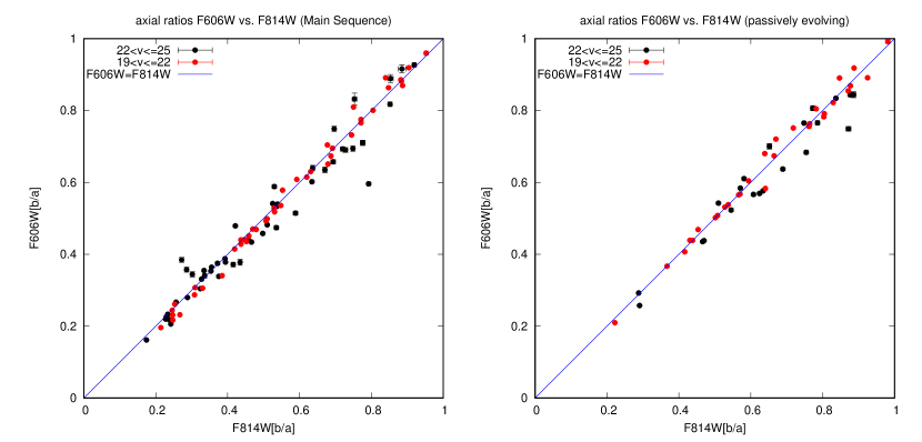
Figure 17: Comparison of the apparent axial ratios measured in the $V_{\rm F606W}$ and $I_{\rm F814W}$ bands for the main-sequence galaxies (left) and passively evolving galaxies (right) at $0.2<z<0.6$. Red symbols show relatively bright galaxies with $V_{\rm F606W}=19$ – 22, while blue symbols show fainter ones with $V_{\rm F606W}=22$ – 25.

Table 4: Comparison of the axial ratios measured in the $V_{\rm F606W}$ and $I_{\rm F814W}$ bands

type	$V_{\rm F606W}$ mag	$N_{\rm obj}$	$(b/a)_{\rm F6060W}-(b/a)_{\rm F814W}$	(error)Δb/a
Main sequence	$V_{\rm F606W}<25$	92	-0.006 $\pm$ 0.037	0.004
	$V_{\rm F606W}<22$	43	-0.003 $\pm$ 0.020	0.002
Passively evolving	$V_{\rm F606W}<25$	51	-0.007 $\pm$ 0.033	0.004
	$V_{\rm F606W}<22$	30	-0.003 $\pm$ 0.022	0.003

4.4.2 Morphological K-correction

We measured the apparent axial ratio on the $I_{\rm F814W}$-band data, which correspond to the rest-frame $V$ band for galaxies at $z\sim 0.4$ and the rest-frame $B$ band for those at $z\sim 0.8$. Such differences in the rest-frame wavelength could cause some biases in the morphological analysis due to the color differences between bulge and disk, the blue star-forming regions/clumps, the dust extinction effect, and so on (e.g., Windhorst et al., 2002; Huertas-Company et al., 2009; Wuyts et al., 2012; Vika et al., 2013; Murata et al., 2014; Mager et al., 2018). In order to check the effects of the morphological K-correction, we used publicly available HST/ACS $V_{F606W}$-band data over a 0.05 deg² region in the COSMOS field from the CANDELS survey (Grogin et al., 2011; Koekemoer et al., 2011). With the $V_{\rm F606W}$-band data, we can measure the apparent axial ratio of galaxies at $0.2<z<0.6$ in the rest-frame $B$ band, and investigate to what extent the difference in the rest-frame wavelength affects the measurements. There are 92 main-sequence and 51 passively evolving galaxies with $V_{\rm F606W}<25$ at $0.2<z<0.6$ in the region, and we measured the apparent axial ratio of these galaxies on the $V_{\rm F606W}$-band data with the same way. In Figure 17, we compare the apparent axial ratios $b/a$ measured on the $V_{\rm F606W}$-band data with those measured on the $I_{\rm F814W}$-band data. The differences between the $V_{\rm F606W}$ and $I_{\rm F814W}$ bands are also summarized in Table 4. The apparent axial ratios measured on the $V_{\rm F606W}$ and $I_{\rm F814W}$-bands data agree well with each other for the both main-sequence and passively evolving populations. The average values of $(b/a)_{F606W}-(b/a)_{F814W}$ are -0.006 and -0.007 for main-sequence and passively evolving galaxies, respectively. These systematic offsets from zero are slightly larger than the averages of the measurement errors, but much smaller than the dispersion around the mean value. When we use only bright subsamples with $V_{\rm F606W}<22$, the results do not significantly change, although the average offsets and measurement errors become slightly smaller. Since these systematic offsets are much smaller than the bin width of 0.1 in the distribution of $b/a$ we used, the morphological K-correction does not significantly affect the distribution of the apparent axial ratio.

4.4.3 Incompleteness

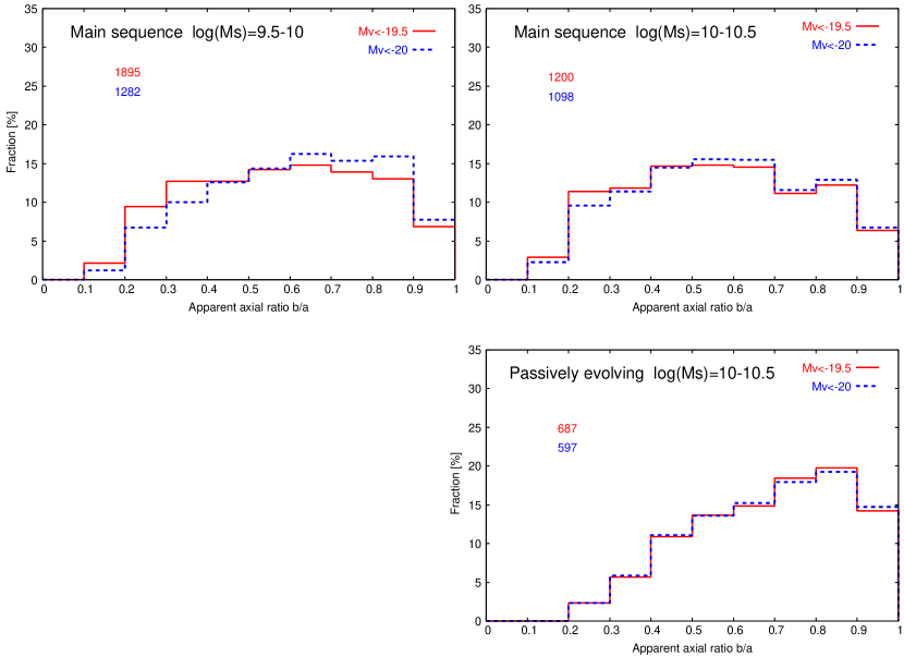
Figure 18: The distribution of the apparent axial ratio for galaxies with $M_{V}<-19.5$ at $0.2<z<0.6$. The top panels show those for the main-sequence galaxies with $M_{\rm star}=10^{9.5}$–$10^{10}M_{\odot}$ (left) and $10^{10}$–$10^{10.5}M_{\odot}$ (right), while the bottom panel shows that for the passively evolving galaxies with $10^{10}$–$10^{10.5}M_{\odot}$. The distribution for galaxies with $M_{V}<-20$ and the same stellar mass, $\Delta$MS, and redshift ranges is also shown in each panel for reference. The total numbers of objects in the subsamples are also shown in each panel.

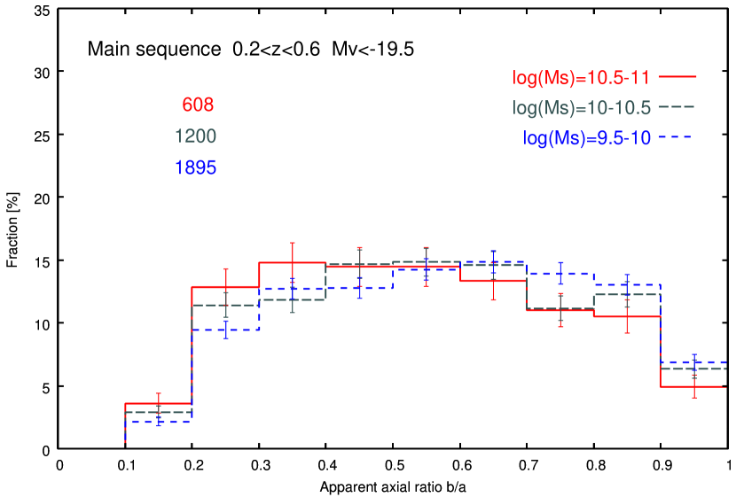
Figure 19: The mass dependence of the distribution of the apparent axial ratio for the main-sequence galaxies with $M_{V}<-19.5$ at $0.2<z<0.6$. The solid, long-dashed, and short-dashed lines represent those galaxies with $M_{\rm star}=10^{10.5}$–$10^{11}M_{\odot}$, $10^{10}$–$10^{10.5}M_{\odot}$, and $10^{9.5}$–$10^{10}M_{\odot}$, respectively. The total numbers of objects in the subsamples are also shown.

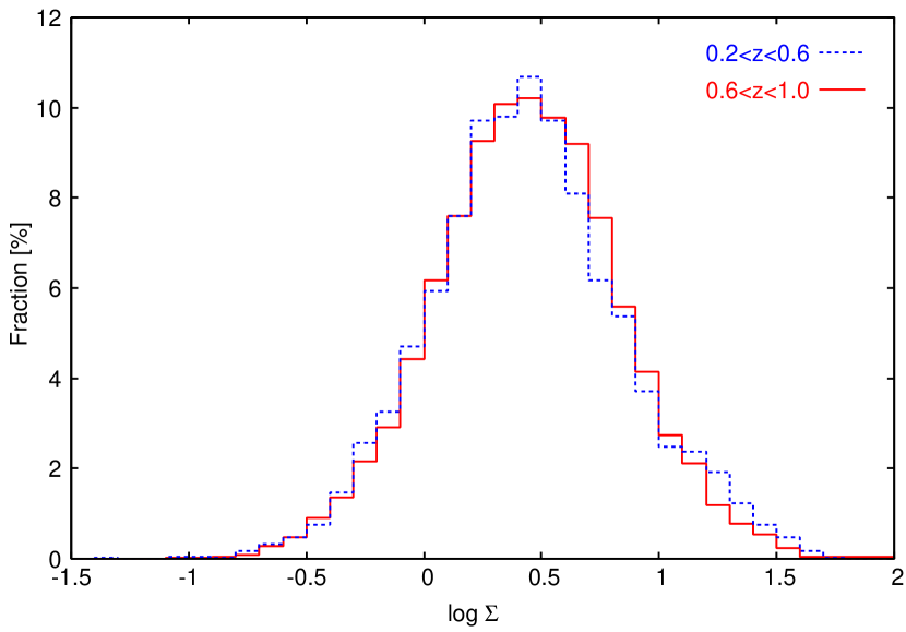
Figure 20: The distributions of the local surface density of our sample galaxies at $0.2<z<0.6$ (blue) and $0.6<z<1.0$ (red) estimated by Darvish et al. (2017). The local density $\Sigma$ is a unit of Mpc^-2 and calculated with the adaptive kernel smoothing and a redshift width of $\pm 1.5\sigma_{\Delta z/(1+z)}$ (see text).

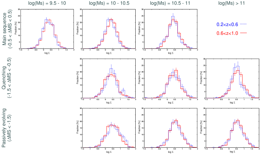
Figure 21: Same as Figure 20, but for subsamples with different stellar mass and $\Delta$MS ranges separately. The configuration of the panels are the same as Figure 9. The error bars are based on the square root of the number of objects in the bin.

In Section 2, we noted that the absolute magnitude limit of $M_{V}<-20$ causes the incompleteness in the low-mass end of our sample especially for those at $0.2<z<0.6$. We missed $\sim 35$ % of the main-sequence galaxies with $10^{9.5}$–$10^{10}M_{\odot}$ at $0.2<z<0.6$ by the limit of $M_{V}<-20$, while $\sim 20$ % of the other galaxies with $10^{10}$–$10^{10.5}M_{\odot}$ at $0.2<z<0.6$ were missed by the same limit (Figure 1). In order to check how the incompleteness affects our results, we measured the apparent axial ratio of those faint galaxies with $-20<M_{V}<-19.5$ at $0.2<z<0.6$ with the same manner. In Figure 18, we show the distributions of the apparent axial ratio of galaxies with $M_{V}<-19.5$ for the main-sequence galaxies with $M_{\rm star}=10^{9.5}$–$10^{10}M_{\odot}$ and $10^{10}$–$10^{10.5}M_{\odot}$, and for the passively evolving galaxies with $10^{10}$–$10^{10.5}M_{\odot}$, and compare them with the results for those with $M_{V}<-20$. The distributions for the main-sequence galaxies with $M_{V}<-19.5$ are slightly skewed toward lower value of $b/a$ compared with those with $M_{V}<-20$ in the both mass ranges. Those faint galaxies with $-20<M_{V}<-19.5$ have systematically lower $b/a$, probably because edge-on star-forming galaxies are more affected by the dust extinction and are systematically fainter at a given stellar mass (e.g, Shao et al., 2007; Padilla, & Strauss, 2008). On the other hand, passively evolving galaxies with $10^{10}$–$10^{10.5}M_{\odot}$ show no significant difference in the distribution between those with $M_{V}<-19.5$ and $M_{V}<-20$. The distribution of those faint galaxies with $-20<M_{V}<-19.5$ is similar with that of brighter galaxies in the passively evolving population.

Figure 19 shows the mass dependence of the axial-ratio distribution for the main-sequence galaxies with $M_{V}<-19.5$. While the distributions for those galaxies with $10^{9.5}$–$10^{10.5}M_{\odot}$ are skewed toward lower values as seen in Figure 18, one can still see that more massive galaxies tend to have lower values of $b/a$. Note that the distribution for those galaxies with $10^{10.5}$–$10^{11}M_{\odot}$ is not affected by the choice of the magnitude limit, because there is only one faint galaxy with $M_{V}>-20$ in the subsample with $10^{10.5}$–$10^{11}M_{\odot}$. Therefore we conclude that the distribution for the main-sequence galaxies really depends on stellar mass, although we probably overestimate the strength of the dependence to some extent due to the incompleteness effect.

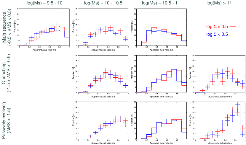
Figure 22: The distributions of the apparent axial ratio for galaxies at $0.2<z<0.6$ located in the different local densities as a function of stellar mass and $\Delta$MS. The configuration of the panels are the same as Figure 9. The red lines show those galaxies in a high-density region with $\Sigma>10^{0.5}$ Mpc^-2, while the blue lines represent those in a lower-density region with $\Sigma<10^{0.5}$ Mpc^-2.

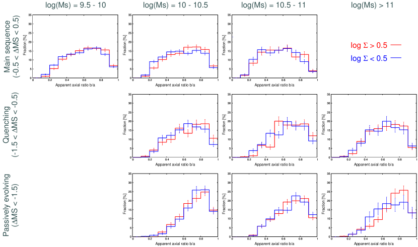
Figure 23: Same as Figure 22, but for galaxies at $0.6<z<1.0$.

4.4.4 Environments

In order to ensure statistical accuracy, we divided our sample by redshift into those at $0.2<z<0.6$ and $0.6<z<1.0$, and have only two redshift bins. Therefore differences of the environments between these two redshift bins could affect our results, although the co-moving survey volumes of these two bins are relatively large ($1.7\times 10^{6}$ Mpc³ for the $0.2<z<0.6$ bin and $4.3\times 10^{6}$ Mpc³ for the $0.6<z<1.0$ bin). If the environments of these two redshift bins are significantly different from each other, we may mainly see the environmental dependence rather than the redshift evolution from the comparisons between these two bins. In order to check this, we investigated the environments of sample galaxies in the two redshift bins by using the local surface number density of galaxies estimated with adaptive kernel smoothing by Darvish et al. (2017). The local number density is calculated with a 2-dimensional Gaussian kernel with a width changing according to the density and the global width is selected to be 0.5 Mpc. In the calculation, they used a redshift width of $\pm 1.5\sigma_{\Delta z/(1+z)}$, which roughly corresponds to be a comoving length of 550–600 Mpc over $0.2<z<1.0$ (Figure 2 of Darvish et al., 2017), and the mean densities over the COSMOS field at $0.2<z<0.6$ and $0.6<z<1.0$ are similar (their Figure 3). Since Darvish et al. (2017) estimated the local number density for galaxies with $M_{\rm star}>10^{9.6}M_{\odot}$ selected in the UltraVISTA field (Laigle et al., 2016), a part of galaxies in our sample are not included in their catalog and unavailable in this analysis. We matched total 19086 objects in our sample (4731 galaxies at $0.2<z<0.6$ and 14355 ones at $0.6<z<1.0$) with those in the catalog by Darvish et al. (2017).

Figure 20 shows the distributions of the local surface number density of galaxies at $0.2<z<0.6$ and $0.6<z<1.0$. While the fraction of galaxies in a high-density region with $\Sigma>10$ Mpc^-2 at $0.6<z<1.0$ is systematically higher than those at $0.2<z<0.6$, the distributions of the local density are basically similar with each other. In Figure 21, we compared the distributions of the local density between the two redshift bins for the subsamples with different stellar mass and $\Delta$MS ranges separately. One can see that more massive galaxies with a lower $\Delta$MS tend to be located in higher-density regions. While star-forming galaxies at $0.6<z<1.0$ seem to be located in slightly higher-density regions than those at $0.2<z<0.6$, there is no large difference in the distribution of the local density between the two redshift bins for all the subsamples. In order to check the environmental dependence of the axial-ratio distribution, we also divided the sample galaxies into those in high-density regions with $\Sigma>10^{0.5}$ Mpc^-2 and those in lower-density regions, and compared the distributions of the apparent axial ratio between these two subsamples at $0.2<z<0.6$ and $0.6<z<1.0$ in Figures 22 and 23, respectively. Although low-mass star-forming galaxies on the main sequence in the high-density regions tend to show slightly higher apparent axial ratios, which indicates thicker intrinsic shapes, than those in lower-density regions, the environmental dependence is not so strong in all the subsamples. By comparing Figures 22 and 23, we confirmed that the passively evolving galaxies with $M_{\rm star}<10^{11}M_{\odot}$ show the significant evolution in their axial-ratio distribution irrespective of environment. We conclude that the differences in the environment between the two redshift bins do not significantly affect our results about the evolution in the axial-ratio distribution.

4.4.5 Size dependence

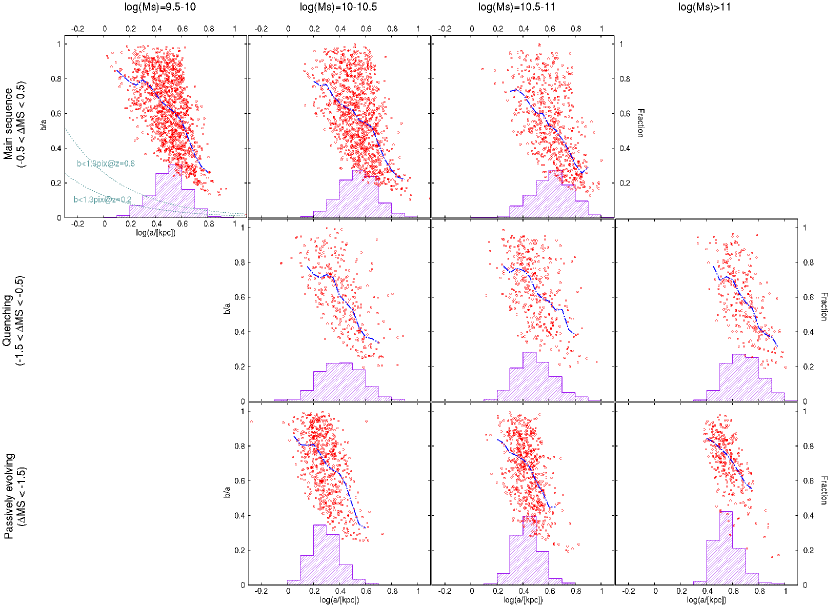
Figure 24: The axial-ratio distribution as a function of semi-major radius for sample galaxies at $0.2<z<0.6$. The blue line shows the median axial ratios in a given size range with a width of 0.1 dex. The histogram represents the size distribution of galaxies in each $M_{\rm star}$ and $\Delta$MS bin. The short dashed curves in the upper left panel show the resolution limit of $b<1.3$ pixel for $z=0.2$ and $z=0.6$.

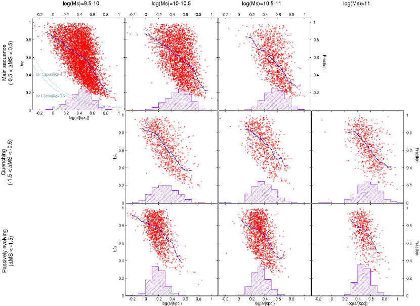
Figure 25: The same as Figure 24, but for galaxies at $0.6<z<1.0$.

Padilla, & Strauss (2008) and Zhang et al. (2019) reported that the axial-ratio distribution of galaxies depends on their sizes. The size dependence could bias our estimate of the 3-dimensional shape from the axial-ratio distribution. Therefore we examine the axial-ratio distribution as a function of size in Figures 24 and 25. We used the semi-major radius $a$ calculated from the second order moment described in Section 3.1 as a size indicator.

The distributions of main-sequence galaxies in the Figures 24 and 25 show similar features with those seen in Zhang et al. (2019) for star-forming galaxies at $0.5<z<1.0$, namely, a curved boundary at the lower left corner, a tail of galaxies at the lower right corner, and a deficiency of galaxies at the upper right corner. As the combination of these features, the median axial ratio of main-sequence galaxies decreases with increasing size. In the upper left panels of the both figures, we also plot the resolution limit of $b<1.3$ pixel described in Section 3.1. The resolution limit does not affect the distribution of galaxies on the $b/a$ vs. $\log{(a)}$ plain.

The axial-ratio distribution for a given size tends to be flat over a wide range of size, and the range of the axial ratio is limited to be higher values at small radii. Although the curved boundary at the lower left corner could be caused by the prolate shape of galaxies (Zhang et al., 2019), the prolate shape leads to a peak around a relatively low value of $b/a$, which is not seen in the observed distributions. Therefore, the observed curved boundary at the lower left corner indicates that the 3-dimensional shape of these galaxies is basically disk-like morphology and their thickness increases with decreasing size. The tail at the lower right is probably caused by the dust extinction effect in edge-on galaxies as discussed in Zhang et al. (2019). When a disk galaxy is viewed in a nearly edge-on view, the central part of galaxies tends to be heavily obscured due to a larger path-length, which leads to the overestimate of the second-order moment along the semi-major axis. On the other hand, the apparent axial ratio $b/a$ is not significantly affected by the dust extinction, because the semi-minor radius along the height direction is similarly overestimated by the dust lane in the edge-on disk. As a result, edge-on disk galaxies whose sizes are overestimated make the tail at the lower right. The fact that the tail is negligible or less significant in passively evolving galaxies with small dust extinction supports this explanation. The deficiency of galaxies at the upper right suggests that the face-on axial ratio $B/A$ is smaller than unity. The deficiency is more significant in massive main-sequence galaxies, which is consistent with the best-fit $\mu_{B/A}$ values of these galaxies seen in Figure 12 and Table 2.

The distribution of passively evolving galaxies similarly shows a curved boundary at the lower left and a deficiency at the upper right, but the distribution for a given size has a peak around $b/a\sim 0.8$, which suggests more thick spheroidal (oblate) shapes. While the curved boundary at the lower left corner and the deficiency at the upper right are naturally expected for such thick spheroidal shapes (Zhang et al., 2019), the concentration of small galaxies at high $b/a$ could reflect such compact galaxies have more spherical shapes than those with larger sizes.

The features of the distribution on the $b/a$ vs. $\log{(a)}$ plain mentioned above are similar among the subsamples with different stellar masses for both main-sequence and passively evolving galaxies, while the size increases with increasing mass for the both populations. These features and the size distributions suggest that the size dependence of the intrinsic shape does not significantly affect the overall axial-ratio distribution in each bin. Therefore, we expect that our estimates for the intrinsic shape of galaxies with $M_{V}<-20$ at $z<1$ are not heavily biased by the size dependence, although those galaxies with smaller sizes tend to have thicker intrinsic shapes and (relatively rare) compact galaxies significantly below the mass-size relation could have systematically spherical shapes.

5 Discussion

5.1 3-dimensional shape transition at $\Delta$MS $\sim-1$ dex

We investigated the distribution of the apparent axial ratio of galaxies with $M_{V}<-20$ at $0.2<z<1.0$ as a function of stellar mass and sSFR, and found that the distribution and estimated intrinsic shape change from the thin disk shape with $C/A\sim$ 0.2 – 0.25 to the thicker spheroidal shape with $C/A\sim$ 0.3 – 0.5 around $\Delta$MS $\sim-1$ dex irrespective of redshift. We discuss possible origins of this transition around $\Delta$MS $\sim-1$ dex in the following.

The major merger is a possible mechanism to cause both the morphological transition and the quenching of star formation. Many previous studies with numerical simulations found that disks of merging galaxies could be destroyed and changed to the spheroidal remnants in the major mergers (e.g., Barnes, 1988; Naab, & Burkert, 2003; Jesseit et al., 2009), while disks may survive in gas-rich major mergers (e.g., Springel, & Hernquist, 2005; Governato et al., 2009). It is also considered that intense starbursts are associated with major mergers through the gas inflow to the galaxy center and/or the gas compression/collapse in the dense tides or clouds, and then the merging remnants could cease star formation due to the gas exhaustion or blowout by the supernova feedback (e.g., Sanders, & Mirabel, 1996; Teyssier et al., 2010; Renaud et al., 2014; see also Sparre, & Springel, 2016). In such major mergers, however, the timescales for the starbursts and the morphological transition seem to vary on a case-by-case basis. For example, Lotz et al. (2008) reported that the enhanced star formation continues after the morphological transition in their simulations. Thus the morphological transition to spheroidal shapes through major mergers does not necessarily occur when sSFR of the remnants corresponds to $\Delta$MS $\sim-1$ dex. Furthermore, if the major merger is the main driver for the shape transition, it may be difficult to explain the observed evolution in the shape of passively evolving galaxies with $M_{\rm star}<10^{11}M_{\odot}$ as discussed in the next section.

The morphological quenching also can cause the decrease of sSFR through the stabilization of the gas disk against the fragmentation to star-forming clumps by the gravity of the dominant bulge (Martig et al., 2009). The bulge growth in star-forming galaxies can be stimulated by minor mergers and/or tidal interactions (e.g., Qu et al., 2011; Guedes et al., 2013; Fiacconi et al., 2015). In this scenario, the morphological transition should precede the quenching of the star formation, and therefore there are bulge-dominated galaxies with a sSFR of the main sequence, i.e., $\Delta$MS $\sim 0$. Morselli et al. (2019) investigated spatially resolved SFR and stellar mass for galaxies at $0.2<z<1.2$ with the multi-band HST data in the GOODS fields. They found that more massive star-forming galaxies on the main sequence are more bulge-dominated, and that those at the lower envelope of the main sequence show more quenched and dominant bulges, which suggests that the bulge growth proceeded on the main sequence. Since the shape of galaxies changes into spheroidal-like before the star formation is quenched in this case, an additional reason is needed to explain the shape transition around $\Delta$MS $\sim-1$ dex. One possibility is that such bulge-dominated galaxies with $\Delta$MS $\sim 0$ is minor in number in galaxies on the main sequence, because there are numerous normal disk-dominated star-forming galaxies. Since these normal disk galaxies are concentrated on the main sequence in sSFR, the bulge-dominated ones become significant in number as their sSFR decreases. If the sSFR at which such quenching galaxies start to dominate corresponds to $\Delta$MS $\sim-1$ dex irrespective of redshift, the shape transition around $\Delta$MS $\sim-1$ dex can be explained.

On the other hand, the quenching of star formation in disks itself through, for example, the morphological quenching mentioned above or environmental effects such as the starvation or the ram-pressure stripping (e.g., Balogh et al., 2000; Abadi et al., 1999) could lead to the changes in the bulge/disk flux ratio. The luminosity of disks is expected to more rapidly decline just after the star formation stopped than that of the passively evolving bulge components. In order to check this effect, we constructed a toy model that consists of a passively evolving bulge and a constantly star-forming and then quenching disk. We used the GALAXEV population synthesis library to estimate the luminosity evolution of the bulge and disk with assumed star formation histories. We assumed that the disk component continued a constant SFR for 3 Gyr and then quenched with timescales with $\tau=$ 1.0 Gyr, 0.5 Gyr, and 0 (abruptly stopped), while the single 1 Gyr burst model with 6 Gyr age when the disk started to quench was adopted for the bulge component (the top panel of Figure 26). The model galaxy has $M_{\rm star}=3.8\times 10^{10}M_{\odot}$ ($M_{\rm bulge}=2.6\times 10^{10}M_{\odot}$ and $M_{\rm disk}=1.2\times 10^{10}M_{\odot}$), $sSFR=10^{-9.75}$ yr^-1, and the disk to total luminosity ratio D/(B+D) $=0.8$ in the rest-frame $B$ band at the quenching of the disk. Figure 26 shows the star formation histories and the rest-frame $B$-band absolute magnitudes of the bulge and disk components, and the disk to total luminosity ratio of the model as a function of time. In the model, sSFR declines by 0.5 and 1 dex for 1.15 (0.58) and 2.3 (1.15) Gyr in the case with a quenching timescale of 1 (0.5) Gyr. The disk becomes fainter by $\sim 1$ mag during the sSFR declines by 1 dex in the cases of $\tau=$ 1 and 0.5 Gyr, which leads to a decrease in the disk fraction from $\sim 0.8$ to $\sim 0.6$. We then carried out a Monte Carlo simulation with the IRAF/ARTDATA package to examine the effect of the decrease of the disk fraction on the axial-ratio distribution. We added artificial objects at $z=0.8$ with the disk and bulge components of the toy model to sky regions in the ACS $I_{\rm F814W}$-band images and measured the apparent axial ratios with SExtractor. The magnitudes, sizes, and axial ratios of the disk and bulge components were adjusted to match with the observed main-sequence and passively evolving galaxies at $0.6<z<1.0$, respectively (see Appendix D for details). We performed 10000 such simulations for the toy model with the disk fraction of 0.8, 0.6, and 0.45 and derived the axial-ratio distribution. Figure 27 shows the results of the simulation. The distribution of the apparent axial ratio for the model with D/(B+D) $=0.6$ are significantly different from that with D/(B+D) $=0.8$. We fitted these axial-ratio distributions with the triaxial ellipsoidal models as described in Section 3.2 and obtained the intrinsic thickness of $\mu_{C/A}=0.23$ and 0.27 for D/(B+D) $=0.8$ and 0.6, respectively. Therefore, we expect that the decrease of the disk fraction due to the quenching of star formation leads to a significant change in the axial-ratio distribution, although the observed change around $\Delta$MS $\sim-1$ dex in Figure 8 may not be fully explained by this effect.

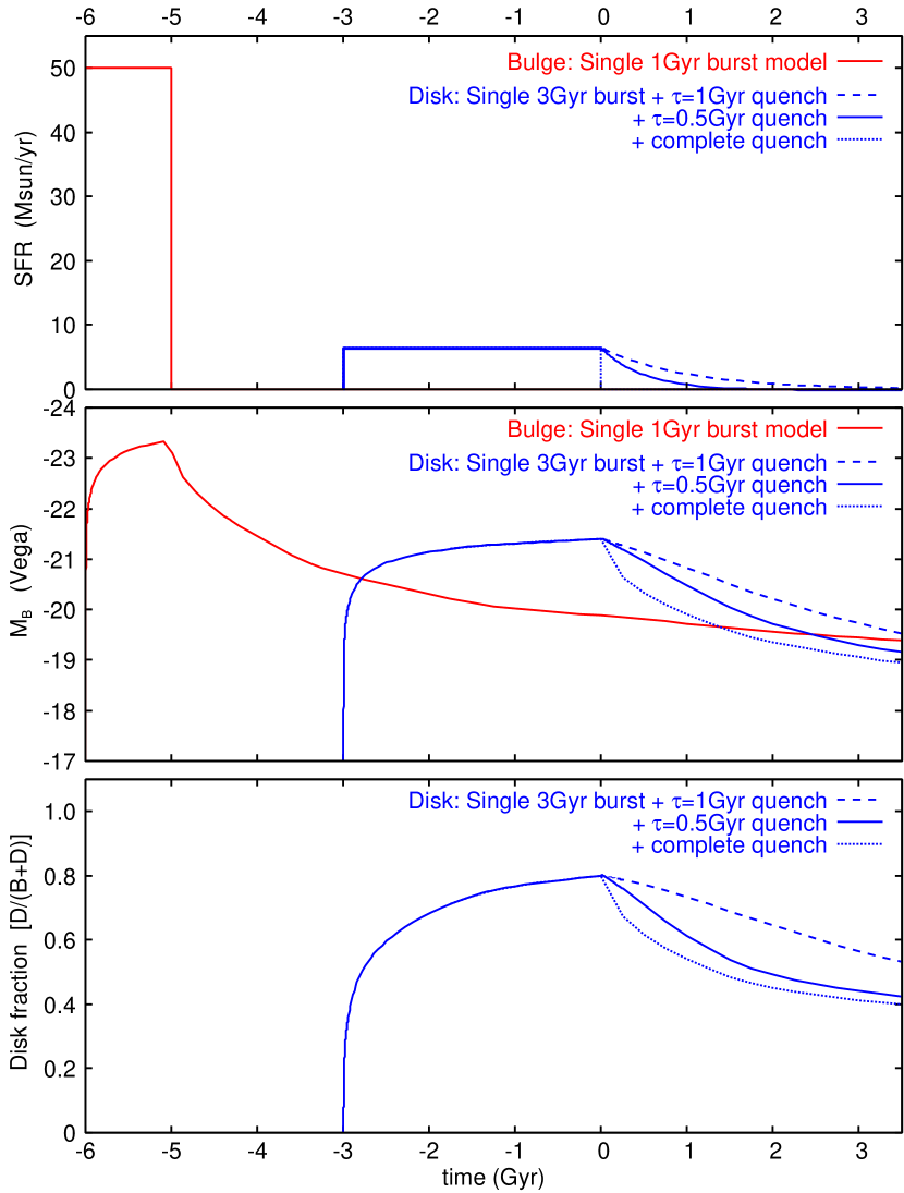
Figure 26: SFR (top), the rest-frame $B$-band absolute magnitude $M_{B}$ (middle), and the disk to total luminosity ratio (bottom) for the disk and bulge components in the toy model as a function of time ($t=0$ at the quenching of the disk). The solid, dashed, and dotted lines show the different quenching timescales for the disk component (see text). The model galaxy has a stellar mass of $3.8\times 10^{10}M_{\odot}$ ($M_{\rm bulge}=2.6\times 10^{10}M_{\odot}$ and $M_{\rm disk}=1.2\times 10^{10}M_{\odot}$) and a sSFR of $10^{-9.75}$ yr^-1 at the quenching of the disk.

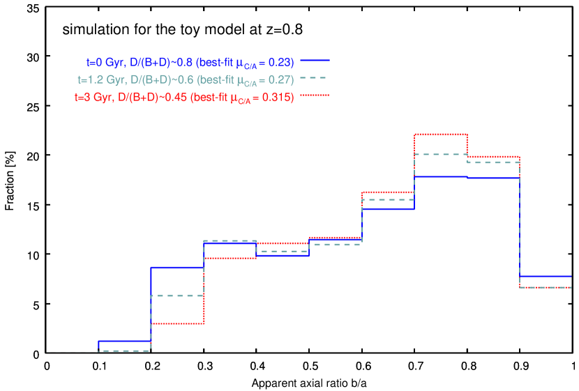
Figure 27: Distribution of the apparent axial ratio for the artificial objects with the different disk fractions. The disk fractions correspond to the ages of the toy model with $\tau=0.5$ Gyr in the legend. The details of the artificial objects added to the $I_{\rm F814W}$-band images are described in Appendix D. The best-fit intrinsic thickness, $\mu_{C/A}$ for each disk fraction is also shown in the legend.

The slightly higher transition sSFR of $\Delta$MS $\sim-0.75$ dex for galaxies with $M_{\rm star}=10^{10.5}$–$10^{11}M_{\odot}$ than those with $10^{10}$–$10^{10.5}M_{\odot}$ may also be explained by this effect, if more massive main-sequence galaxies tend to have the high bulge fraction as shown by Morselli et al. (2019). Bremer et al. (2018) carried out the multi-component surface brightness fitting for galaxies with $M_{\rm star}=10^{10.25}$–$10^{10.75}M_{\odot}$ at $z<0.2$ from the GAMA survey with the multi-band data, and found that most of green-valley galaxies show significant bulge and disk components. They also suggested that the migration from the blue cloud to the red sequence is caused by the disk fading.

5.2 Shape evolution of passively evolving galaxies at $z<1$

In Section 4.2, we found that the distribution of the apparent axial ratio and intrinsic shape of passively evolving galaxies with $M_{\rm star}<10^{11}M_{\odot}$ significantly evolve between $z\sim 0.8$ and $z\sim 0.4$; the edge-on axial ratio $C/A$ (thickness) decreases with time from $\mu_{C/A}=0.500$ (0.400) at $0.6<z<1.0$ to $\mu_{C/A}=0.370$ (0.325) at $0.2<z<0.6$ for those with $M_{\rm star}=10^{10}$–$10^{10.5}M_{\odot}$ ($10^{10.5}$–$10^{11}M_{\odot}$). On the other hand, massive galaxies with $M_{\rm star}>10^{11}M_{\odot}$ have a thick shape with $\mu_{C/A}=$ 0.45 – 0.49 and show no significant evolution in their shape.

van der Wel et al. (2009) and Holden et al. (2012) measured the apparent axial ratio of quiescent galaxies at $z=$ 0.04 – 0.08 with the SDSS data, and found that massive galaxies with $M_{\rm star}>10^{11}M_{\odot}$ exclusively have $b/a>0.6$, while those galaxies with $M_{\rm star}<10^{11}M_{\odot}$ show more flatter distribution over $b/a=$ 0.2 – 1.0. These results are consistent with those of passively evolving galaxies at $0.2<z<0.6$ in this study. Holden et al. (2012) also investigated the axial-ratio distribution of quiescent galaxies at $z=$ 0.6 – 0.8 with the GEMS and COSMOS data, and confirmed that these galaxies show the similar trends with the SDSS galaxies at $z\sim 0.06$, which is consistent with our results for those at $0.6<z<1.0$. Although they found no significant evolution between $z\sim 0.7$ and $z\sim 0.06$ for quiescent galaxies with $M_{\rm star}<10^{11}M_{\odot}$, their sample size for $z\sim 0.7$ galaxies is $\sim$ 2–3 times smaller than our sample at $0.6<z<1.0$. The differences between passively evolving galaxies at $0.2<z<0.6$ and $0.6<z<1.0$ in the axial-ratio distribution in Figure 9 would be buried in noise especially for those galaxies with $M_{\rm star}=10^{10.5}$–$10^{11}M_{\odot}$, if we decrease the sample size by a factor of $\sim$ 2 – 3. Hill et al. (2019) studied the median values of the apparent axial ratio for quiescent and star-forming galaxies at $0.2<z<4.0$ with the CANDELS/3D-HST data. They found that low-mass quiescent galaxies with $M_{\rm star}<10^{10.5}M_{\odot}$ show a evolution of the median axial ratio from $\sim 0.68$ at $0.5<z<1.0$ to $\sim 0.63$ at $0.2<z<0.5$, while no significant evolution is seen for those with $M_{\rm star}>10^{10.5}M_{\odot}$. The result for those low-mass galaxies seems to be consistent with our result, although those with $M_{\rm star}=10^{10.5}$–$10^{11}M_{\odot}$ show no significant evolution in Hill et al. (2019) probably due to a relatively small number of their samples (total $\sim 800$ and 200 quiescent galaxies at $0.5<z<1.0$ and $0.2<z<0.5$ before divided by stellar mass).

In our results, the thickness (edge-on axial ratio $C/A$) of passively evolving galaxies with $M_{\rm star}=10^{10}$–$10^{11}M_{\odot}$ decreases with time on average. In general, it is difficult to make a stellar disk system thinner without forming new stars from a thin gas disk, because such a stellar disk system once formed tends to become thicker shape as time passes through minor mergers, galaxy interactions, and so on (e.g., Quinn et al., 1993; Villalobos, & Helmi, 2008). The minor merger/interaction could stimulate the bulge growth (Qu et al., 2011), which also leads to the thicker shape of those galaxies. Since the increase in the number density of passively evolving galaxies at $z\lesssim 1$ is much larger than that of star-forming galaxies (e.g., Borch et al., 2006; Ilbert et al., 2010), most quiescent galaxies are expected not to experience a significant star formation after the star formation once stopped (e.g., Bell et al., 2007; but see also Mancini et al., 2019). Thus passively evolving galaxies quenched in earlier epoch do not seem to evolve into thinner shape with time.

On the other hand, star-forming galaxies on the main sequence at $0.2<z<1.0$ have much thinner shapes with $\mu_{C/A}=$ 0.2 – 0.25 (Figure 11 and Table 2). Therefore, newly quenching galaxies from the main-sequence population could cause the evolution of the axial-ratio distribution for the passively evolving population, if their morphology does not violently change during the quenching. For example, while the disk fading and/or bulge growth mentioned in the previous section make the thickness of the newly quenching galaxies slightly larger than the typical value of main-sequence galaxies, such galaxies could be still sufficiently thinner than passively evolving ones quenched in earlier epoch. Carollo et al. (2013) investigated the number density evolution of passively evolving galaxies at $0.2<z<1.0$ in the COSMOS field as a function of galaxy size, and found that the fraction of those galaxies with a larger size increases with time. Since those galaxies with a larger size have slightly bluer rest-frame $U-V$ colors than those with a normal size, they suggested that newly quenching galaxies with a larger size mainly cause the evolution in the size distribution of passively evolving galaxies. The scenario mentioned above seems to be consistent with the results by Carollo et al. (2013), because star-forming galaxies tend to show larger sizes than passively evolving galaxies at a given stellar mass at $z\lesssim 3$ (e.g., van der Wel et al., 2014b). Newly quenching galaxies from the main sequence are expected to have both a thinner shape and a larger size. In fact, from Figures 24 and 25, we can see that (1) passively evolving galaxies tend to have smaller sizes than star-forming ones with the same mass and redshift, (2) passively evolving galaxies with larger sizes tend to show more extended axial-ratio distributions down to lower $b/a$ values, and (3) the sizes of passively evolving galaxies for a given mass significantly increase with time. These trends are consistent with the scenario. In this scenario, the major merger, which tends to destroy the thin disk component, cannot be the main driver of the quenching of star formation, although a relatively small fraction of galaxies may quench through the major merger.

The transition of newly quenching galaxies with a thin shape from the main-sequence population could also explain the stellar mass dependence of the evolution in the axial-ratio distribution of passively evolving galaxies. The evolution of the galaxy stellar mass function for quiescent galaxies in previous studies suggests that the number density increase with time at $z\lesssim 1$ in the passively evolving population is larger for less massive galaxies at $M_{\rm star}<10^{11}M_{\odot}$ (e.g., Ilbert et al., 2010; Ilbert et al., 2013; Muzzin et al., 2013). Thus the expected fraction of galaxies newly quenched between $z\sim 0.8$ and $z\sim 0.4$ in the passively evolving population is higher for less massive galaxies. This can explain the result that passively evolving galaxies with $M_{\rm star}=10^{10}$–$10^{10.5}M_{\odot}$ show the stronger evolution of the thickness from $\mu_{C/A}=0.50$ at $0.6<z<1.0$ to 0.37 at $0.2<z<0.6$ than those with $10^{10.5}$–$10^{11}M_{\odot}$ (from $\mu_{C/A}=$ 0.40 to 0.33).

In this scenario, the relatively thick spheroidal shapes of passively evolving galaxies with $M_{\rm star}<10^{11}M_{\odot}$ at $0.6<z<1.0$ could be explained at least partly by a lack of the supply of quenching galaxies with a thin shape at higher redshifts, because star-forming galaxies at $z>1$ seem to have thicker shapes than those at $z<1$. Several studies have investigated the apparent axial ratios of star-forming galaxies at $z>1$ with the optical/NIR HST data to estimate their intrinsic shapes, and found that these galaxies at $z\sim$ 1.5–3 have thicker and more prolate (bar-like) shapes (Ravindranath et al., 2006; Yuma et al., 2011; Yuma et al., 2012; Law et al., 2012; van der Wel et al., 2014a; Takeuchi et al., 2015; Zhang et al., 2019). Ground-based observational studies with the integral field spectroscopy also found that star-forming galaxies with a rotationally supported disk at $z\sim 2$ show larger velocity dispersion than disk galaxies at lower redshifts, which suggests thicker shape of the disk (e.g., Förster Schreiber et al., 2009; Law et al., 2012; Wisnioski et al., 2015). Therefore galaxies with a very thin shape seem to be rare at such high redshift even in the star-forming population, and it is difficult to form passively evolving galaxies with such a thin shape at $z>1$. The higher merger rate at higher redshifts (e.g., Mundy et al., 2017; Duncan et al., 2019) could also contribute to more thicker shapes of those high-redshift galaxies.

On the other hand, no significant evolution in the shape of massive passively evolving galaxies with $M_{\rm star}>10^{11}M_{\odot}$ can be explained by a lack of such massive star-forming galaxies irrespective of shape. The stellar mass function for star-forming galaxies indicates that massive star-forming galaxies with $M_{\rm star}>10^{11}M_{\odot}$ are very rare at $z\lesssim 1$ (e.g., Ilbert et al., 2013; Muzzin et al., 2013), and the expected number of such massive galaxies that newly quench the star formation without major mergers between $z\sim 0.8$ and $z\sim 0.4$ is very small. Instead, massive passively evolving galaxies with $M_{\rm star}>10^{11}M_{\odot}$ are expected to be mainly formed through the major mergers of relatively massive objects with $M_{\rm star}\sim 10^{11}M_{\odot}$. Since the quiescent fraction in galaxies with $M_{\rm star}\sim 10^{11}M_{\odot}$ becomes relatively high at $z\lesssim 1$ (e.g., Ilbert et al., 2010; Kajisawa et al., 2011), such major mergers tend to be dry mergers or those with a relatively low gas-mass fraction, which leads to the spheroidal shapes of the remnants (e.g., Springel, & Hernquist, 2005; Hopkins et al., 2009; Rodriguez-Gomez et al., 2017). The lack of newly quenching galaxies with a thin shape and the formation through dry major mergers can explain the thick spheroidal shape and its no significant evolution at $z<1$ for passively evolving galaxies with $M_{\rm star}>10^{11}M_{\odot}$ (Holden et al., 2012). The flatter shapes of massive quiescent galaxies with $M_{\rm star}>10^{11}M_{\odot}$ at $z>1$ reported by Chang et al. (2013) and Hill et al. (2019) could be explained similarly by their formation through the wet mergers, because the merger progenitors are expected to be more gas-rich at higher redshifts.

5.3 Stellar mass dependence of thickness and its imprecations

We found that the intrinsic edge-on axial ratio $C/A$ of main-sequence galaxies decreases with increasing stellar mass in the both redshift ranges (Figure 12 and Table 2). Recently, Pillepich et al. (2019) investigated the 3-dimensional shapes of stellar and gaseous components of star-forming galaxies in the high-resolution cosmological simulation, Illustris TNG50, and found that more massive star-forming galaxies show lower edge-on axial ratio $C/A$, i.e., thinner shapes of the stellar component than less massive galaxies at $0.5<z<4.0$. Their results for the thickness of those galaxies at $z\sim 0.5$ as a function of stellar mass are qualitatively consistent with our results, although a direct comparison is difficult due to the different stellar mass and redshift binning between Pillepich et al. (2019) and this study. In their simulation, the gas disks strongly evolve into thinner shapes as the $V_{\rm rot}/\sigma$ of the gas disk significantly decreases with time, and the star formation in the thin gas disk makes the stellar disk thinner. The thickness of the gas disk at a given redshift tends to be smaller in more massive star-forming galaxies in all redshifts, which leads to the mass dependence of the thickness of the stellar disk. On the other hand, Sales et al. (2012) found that the coherent alignment of the angular momentum of gas that has been accreting onto a galaxy over time is more important for the formation of the thin-disk morphology than the net spin or merger history of the dark matter halo the galaxy resides in the GIMIC cosmological simulation. They also suggested that gas accretion from a quasi-hydrostatic hot corona, namely, “hot-mode” accretion preferentially forms a thin stellar disk, because such shock-heated gas in the halo is forced to homogenize its rotation properties before accreting onto the galaxy, which results in a rather gradual supply of gas with a relatively stable spin axis. In contrast with the hot-mode accretion, cold gas accretion, where gases from distinct filaments directly flow into the central galaxy with misaligned spins, tends to disturb the gas kinematics and form a more thick spheroidal stellar component. The hot-mode accretion is expected to dominate preferentially in more massive dark matter halo with $M_{\rm halo}\gtrsim 10^{11.5}M_{\odot}$ from the previous theoretical studies (e.g., Birnboim, & Dekel, 2003; Kereš et al., 2005). It is suggested by the clustering and/or abundance matching analyses that more massive star-forming galaxies tend to be associated with more massive dark matter halos (e.g., Tinker et al., 2013; Legrand et al., 2019). Therefore, the stellar mass dependence of the thickness of star-forming galaxies could be explained by the halo mass dependence of the contribution from the hot mode accretion in the gas supply to the galaxies. In fact, Legrand et al. (2019) found that the dark matter halo mass of star-forming galaxies at $0.2\lesssim z\lesssim 1$ increases with stellar mass from $\sim 10^{11.3}$–$10^{11.7}M_{\odot}$ at $M_{\rm star}\sim 10^{9.5}M_{\odot}$ to $\sim 10^{12.3}-10^{12.7}M_{\odot}$ at $M_{\rm star}\sim 10^{11}M_{\odot}$, where the contribution from the hot mode accretion is expected to increase with halo mass. More massive star-forming galaxies on the main sequence tend to be formed in massive halos dominated by the hot mode accretion, which may leads to their observed thinner shapes.

This scenario could also explain the reason why star-forming galaxies with a relatively thin disk appeared around $z\sim 1$, because the hot mode accretion is expected not to dominate even in massive halos at $z\gtrsim 2$ due to gas supply through the cold gas stream (e.g., Kereš et al., 2009; Dekel et al., 2009a). Some of gas accreting to a dark matter halo is expected to penetrate surrounding hot gas in a form of filaments of dense and cold infalling gas and directly accrete onto the central galaxy at such high redshift, where the mass accretion rate and matter density tend to be high. Such direct gas supply through the filaments of cold gas could make the gas disk of the central galaxy more turbulent and gravitationally unstable, which leads to thick and clumpy stellar disk and bulge formation/growth in some cases (e.g., Dekel et al., 2009b; Ceverino et al., 2010; Dekel, & Burkert, 2014). Thus it seems to be difficult to form the thin stellar disks even in massive halos at $z\gtrsim 2$. After the hot-mode accretion starts to dominate at $z\sim 2$ in relatively massive halos, the thin stellar disks may be gradually formed from thinner gas disks and appear around $z\sim 1$. If some of these star-forming galaxies with a thin stellar disk quench and evolve into passively evolving galaxies without a violent morphological change as discussed in the previous section, it is understood that the fraction of passively evolving galaxies with a thin shape increases with time at $z<1$ rather than higher redshifts. Since more massive star-forming galaxies have a sufficient time to form a thin disk through the hot mode accretion in earlier epoch in this scenario (Noguchi, 2019), passively evolving galaxies with a thin shape may also be provided preferentially in more massive galaxy population at $z\sim 1$. This could explain our result that passively evolving galaxies with $M_{\rm star}=10^{10.5}$–$10^{11}M_{\odot}$ already show a thinner shape than those with $10^{10}$–$10^{10.5}M_{\odot}$ at $0.6<z<1.0$. In fact, Bezanson et al. (2018) reported that $\sim 64$% of quiescent galaxies with $M_{\rm star}\sim 10^{10.5}$–$10^{11}M_{\odot}$ at $0.6<z<1.0$ show a significant rotation, while those massive galaxies with $M_{\rm star}>10^{11}M_{\odot}$ show no or little rotation in the LEGA-C survey. Such quiescent galaxies with a significant rotation might be recently quenched galaxies with a relatively thin disk that has grown through the hot mode gas accretion since $z\lesssim$ 2.

6 Summary

With the COSMOS HST/ACS $I_{\rm F814W}$-band data over the 1.65 deg² region in the COSMOS field, we measured the apparent axial ratios of $\sim$ 21000 galaxies with $M_{V}<-20$ at $0.2<z<1.0$, and fitted the distribution of the axial ratio with the triaxial ellipsoid models to statistically estimate their intrinsic 3-dimensional shapes as a function of stellar mass, sSFR, and redshift. Our main results are summarized as follows.

• We confirmed that star-forming galaxies on the main sequence show a thin disk shape with a intrinsic edge-on axial ratio of $C/A\sim$ 0.2 – 0.25, while passively evolving galaxies with a low sSFR have a more thick spheroidal shape with $C/A\sim$ 0.3 – 0.5.

• The transition from the thin disk to the thick spheroidal shape for galaxies with $M_{\rm star}=10^{10}$–$10^{11}M_{\odot}$ occurs around $\Delta$MS $\sim-1$ dex, i.e., an order of magnitude lower sSFR than that of the main sequence irrespective of redshift. The shape of galaxies with $M_{\rm star}=10^{10.5}$–$10^{11}M_{\odot}$ changes at slightly higher $\Delta$MS ($\sim-0.75$ dex) than that of less massive ones with $10^{10}$–$10^{10.5}M_{\odot}$ ($\sim-1$ dex).

• Passively evolving galaxies with $M_{\rm star}<10^{11}M_{\odot}$ show a significant evolution in the axial-ratio distribution and estimated intrinsic shape. The edge-on axial ratio $C/A$ decreases with time from $\mu_{C/A}=0.500$ (0.400) at $0.6<z<1.0$ to $\mu_{C/A}=0.370$ (0.325) at $0.2<z<0.6$ for those galaxies with $M_{\rm star}=10^{10}-10^{10.5}M_{\odot}$ ($10^{10.5}$–$10^{11}M_{\odot}$). On the other hand, those massive galaxies with $M_{\rm star}>10^{11}M_{\odot}$ have a thick shape with $\mu_{C/A}=$ 0.45 – 0.49 and show no significant evolution in their shape at $0.2<z<1.0$.

• The intrinsic shape of star-forming galaxies on the main sequence does not significantly evolve at $0.2<z<1.0$. On the other hand, the intrinsic edge-on axial ratio $C/A$ (thickness) of the main-sequence galaxies decreases with increasing stellar mass from $\mu_{C/A}=0.265$ (0.255) for galaxies with $M_{\rm star}=10^{9.5}$–$10^{10}M_{\odot}$ at $0.2<z<0.6$ ($0.6<z<1.0$) to $\mu_{C/A}=0.210$ (0.230) for those with $10^{10.5}$–$10^{11}M_{\odot}$, although the uncertainty is not negligible.

We discussed that the quenching and migration to the passively evolving population of some main-sequence galaxies with a thin shape without violent morphological change can explain the shape transition at a nearly constant $\Delta$MS and the evolution of the fraction of passively evolving galaxies with a thin shape at $M_{\rm star}<10^{11}M_{\odot}$. The scenario that the thin stellar disks of star-forming galaxies are formed by the gas supply through the hot-mode accretion could also explain the stellar mass dependence of the thickness of these galaxies and the increase of the fraction of passively evolving galaxies with a thin shape at $z<1$. On the other hand, massive passively evolving galaxies with $M_{\rm star}>10^{11}M_{\odot}$ are expected to be formed by dry major mergers at $z<1$, which leads to thick and spheroidal shapes.

The statistical analysis of the apparent axial ratio such as this study is a powerful tool to constrain the evolution in the intrinsic shape, especially thickness of galaxies over the cosmic time, but its advantage strongly depends on the sample size. The future wide-field surveys with JWST and WFIRST will enable us to investigate the evolution more detailedly with high statistical accuracy.

Appendix A Examples of sample galaxies as a function of axial ratio

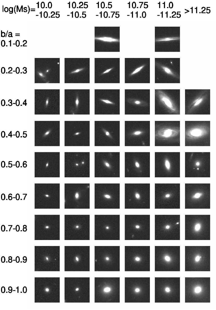
Figure 28: Examples of passively evolving galaxies with $\Delta$MS $<-1.5$ dex at $0.2<z<0.6$ in our sample as a function of axial ratio and stellar mass. The apparent axial ratio of the object increases from top to bottom row, and the stellar mass increases from left to right column. Each panel is $6^{\prime\prime}\times 6^{\prime\prime}$ in size. These galaxies are randomly selected in the axial ratio and stellar mass bins. Note that there is no sample galaxy in some of the bins at $b/a<0.3$.

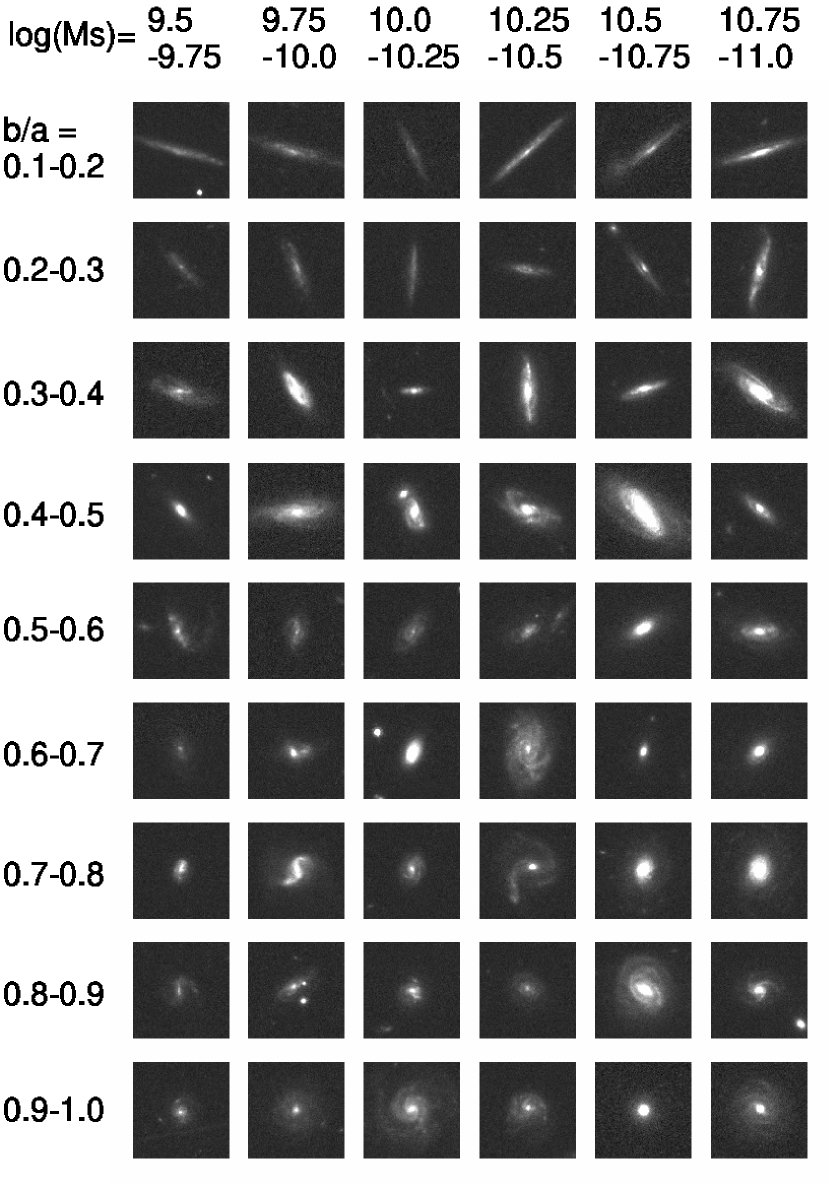
Figure 29: Same as Figure 28, but for star-forming galaxies on the main sequence with $\Delta$MS $=-0.5$ – $+0.5$ at $0.2<z<0.6$.

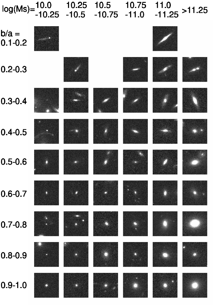
Figure 30: Same as Figure 28, but for passively evolving galaxies with $\Delta$MS $<-1.5$ dex at $0.6<z<1.0$.

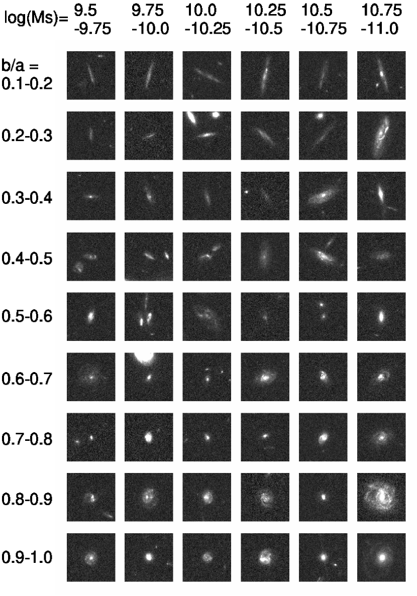
Figure 31: Same as Figure 28, but for star-forming galaxies on the main sequence at $0.6<z<1.0$.

We show HST/ACS $I_{\rm F814W}$-band images of some sample galaxies with different sSFRs and redshifts as a function of the measured axial ratio in Figures 28–31. Note that galaxies with a low sSFR of $\Delta$MS $<-1.5$ dex tend to show relatively large apparent axial ratios, and there are few those galaxies with a very small axial ratio of $b/a\lesssim 0.2$.

Appendix B The best-fit models for the subsamples

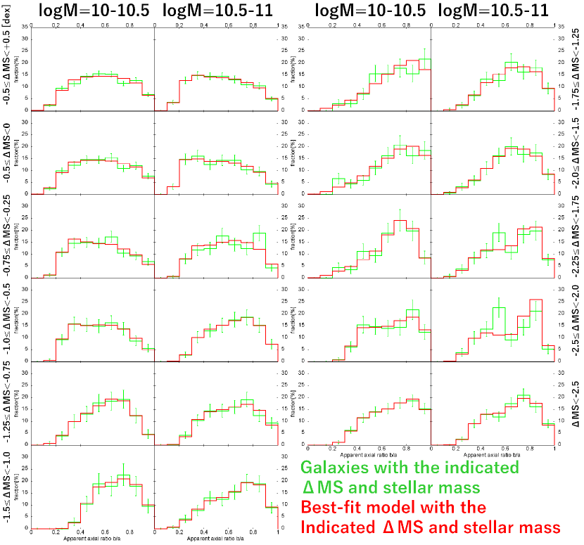
Figure 32: The observed distribution of the apparent axial ratio and the best-fit triaxial ellipsoid models described in Section 3.2 for the subsamples at $0.2<z<0.6$ as a function of $\Delta$MS and stellar mass. The configuration of the panels are the same as Figure 6.

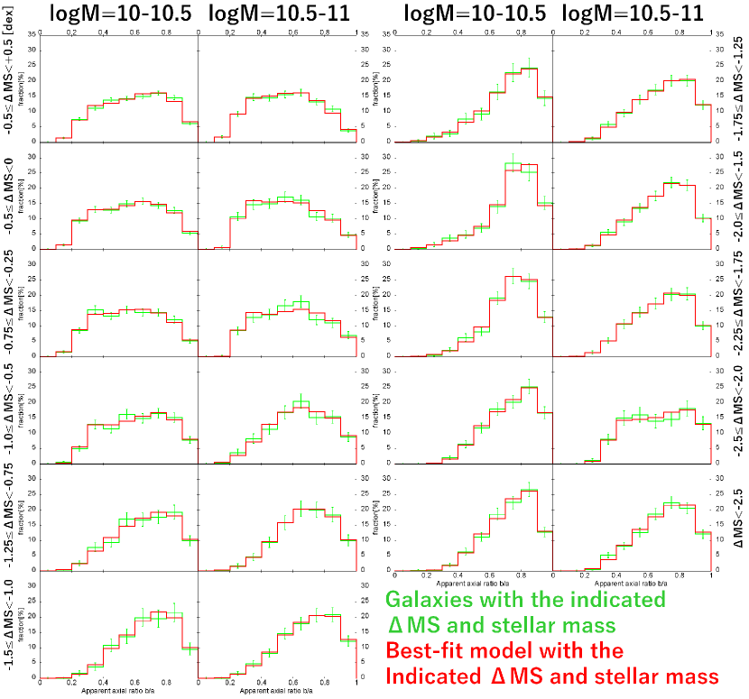
Figure 33: The same as Figure 32, but for galaxies at $0.6<z<1.0$.

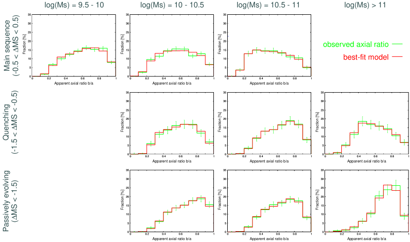
Figure 34: The observed distribution of the apparent axial ratio and the best-fit model for the subsamples at $0.2<z<0.6$ as a function of $\Delta$MS and stellar mass. The samples are divided by $\Delta$MS into the main-sequence, quenching, and passively evolving populations. The configuration of the panels are the same as Figure 9.

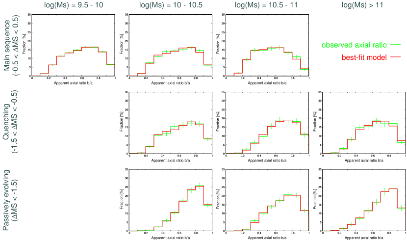
Figure 35: The same as Figure 34, but for galaxies at $0.6<z<1.0$.

In this study, we fitted the distribution of the apparent axial ratio for the subsamples with various stellar mass and $\Delta$MS ranges with the triaxial ellipsoid models to estimate the intrinsic 3-dimensional shape. We show comparisons between the observed axial-ratio distributions and the best-fit models for the subsamples used in this study in Figures 32–35, which enable to examine the goodness of fitting for each subsample and check whether the systematic difference between the observed distribution and the best-fit model exists or not. One can see that the observed distributions are well fitted by the models for all the subsamples and there seems to be no systematic difference.

Appendix C The model fitting for galaxies with $M_{\rm star}=10^{10}$–$10^{10.5}M_{\odot}$ and $\Delta$MS $\sim-2.0$ – $-1.5$ at $0.2<z<0.6$

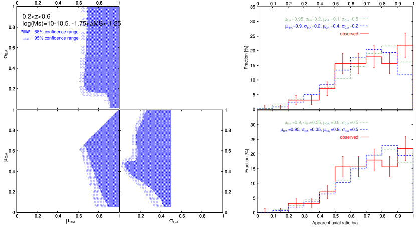
Figure 36: (left) The confidence ranges of the intrinsic shape parameters, namely, $\mu_{B/A}$, $\sigma_{B/A}$, $\mu_{C/A}$, and $\sigma_{C/A}$, in the fitting of the observed axial-ratio distribution for galaxies with $M_{\rm star}=10^{10}$–$10^{10.5}M_{\odot}$ and $\Delta$MS $=-1.75$ – $-1.25$ dex at $0.2<z<0.6$. (right) The observed axial-ratio distribution (solid line) and the acceptable models with various values of the fitting parameters within the 68% confidence ranges for the same subsample (dashed lines).

Figure 37: The same as Figure 36 but for galaxies with $M_{\rm star}=10^{10}$–$10^{10.5}M_{\odot}$ and $\Delta$MS $=-2.0$ – $-1.5$ dex at $0.2<z<0.6$.

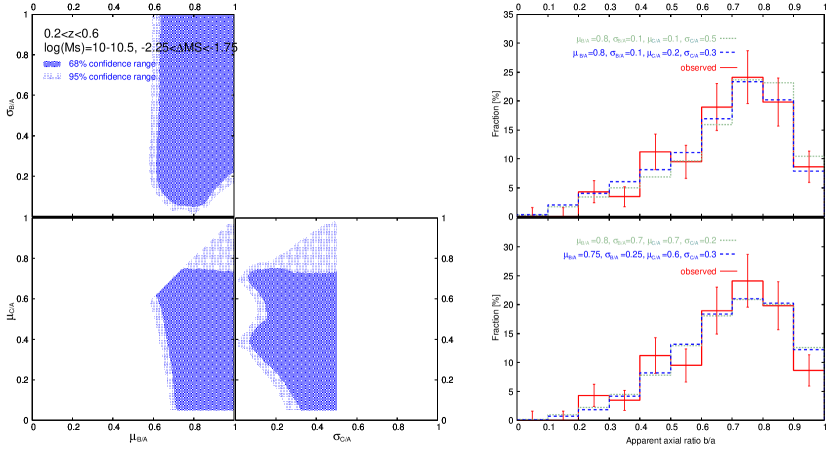
Figure 38: The same as Figure 36 but for galaxies with $M_{\rm star}=10^{10}$–$10^{10.5}M_{\odot}$ and $\Delta$MS $=-2.25$ – $-1.75$ dex at $0.2<z<0.6$.

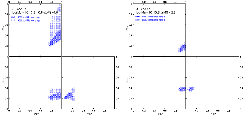
Figure 39: The confidence ranges of the intrinsic shape parameters in the fitting of the observed axial-ratio distribution for galaxies with $M_{\rm star}=10^{10}$–$10^{10.5}M_{\odot}$ and $\Delta$MS $=-0.5$ – $+0.5$ dex at $0.2<z<0.6$ (left) and for those with $\Delta$MS $<-2.5$ dex in the same stellar mass and redshift range (right).

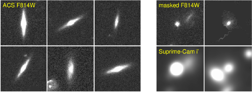
Figure 40: Examples of galaxies with $b/a=0.2$ – 0.3, $M_{\rm star}=10^{10}$–$10^{10.5}M_{\odot}$, and $\Delta$MS $=-2.25$ – $-1.25$ dex at $0.2<z<0.6$. The left panels show the ACS $I_{\rm F814W}$-band images of edge-on disk galaxies with a significant bulge. The right panels show examples of galaxies whose axial ratios are affected by nearby objects. While the top panels show the $I_{\rm F814W}$-band images where nearby objects are masked out, the bottom panels represent the Suprime-Cam $i^{\prime}$-band images of the same objects, where the source detection were performed. The all images are $6^{\prime\prime}\times 6^{\prime\prime}$ in size.

We here examine the model fitting for the axial-ratio distribution of galaxies with $M_{\rm star}=10^{10}$–$10^{10.5}M_{\odot}$ and $\Delta$MS $\sim-2.0$ – $-1.5$ dex at $0.2<z<0.6$, where the uncertainty of $\mu_{C/A}$ is very large. The left panels of Figures 36, 37, and 38 show the confidence ranges of the fitted intrinsic shape parameters, $\mu_{B/A}$, $\sigma_{B/A}$, $\mu_{C/A}$, and $\sigma_{C/A}$ for galaxies with $\Delta$MS $=-1.75$ – $-1.25$, $-2.0$ – $-1.5$, and $-2.25$ – $-1.75$ dex, respectively. One can see that the constraints on $\mu_{C/A}$ and $\sigma_{B/A}$ are very weak in the fittings for these galaxies. Relatively higher values of $\sigma_{C/A}\gtrsim 0.2$ are preferred in the fitting for these galaxies, while $\sigma_{C/A}$ tends to be constrained to lower values in the fitting for the other subsamples, for example, those with $\Delta$MS $=-0.5$ – $+0.5$ and $\Delta$MS $<-2.5$, whose all parameters are well constrained (Figure 39). The right panels of Figures 36, 37, and 38 show the observed axial-ratio distributions for these galaxies and those of acceptable models with various values of the fitting parameters within the 68% confidence ranges. The observed distributions for these galaxies have both a broad peak around $b/a\sim 0.8$ – 1.0 and a non-negligible fraction of galaxies at $b/a=0.2$ – 0.3. Such distributions are difficult to be reproduced by the models with a small $\sigma_{C/A}$, because in such cases with small $\sigma_{C/A}$ the broad peak around $b/a\sim 0.8$ – 1.0 requires a relatively high value of $\mu_{C/A}$ (and $\mu_{B/A}$), which leads to a very small fraction of those with $b/a<0.3$. On the other hand, the models with a large $\sigma_{C/A}$ could roughly reproduce such distributions (the right panels of Figures 36, 37, and 38). In the models with a large $\sigma_{C/A}$, $C/A$ are widely distributed irrespective of $\mu_{C/A}$ and the effects of $\mu_{C/A}$ on the shape of the axial-ratio distribution tend to be relatively small. This seems to be one of the reasons for the large acceptable range of $\mu_{C/A}$ in the fitting of these galaxies as well as the large statistical uncertainty of the observed distributions due to the small size of the subsamples. We also note that there are some acceptable models with a relatively small value of $\sigma_{C/A}\lesssim 0.2$ in the left panels in Figures 36, 37, and 38. In such cases, a large value of $\sigma_{B/A}$ is needed to match with the observed distributions (the bottom right panel of Figure 38).

While most of those galaxies with $b/a=0.2$ – 0.3 and $\Delta$MS $\sim-2.25$ – $-1.25$ dex are edge-on disk galaxies with a significant bulge, there are a few galaxies with a relatively round shape that affected by a nearby faint elongated companion or the outer part of nearby bright objects (Figure 40). For these objects, we could not completely mask out the nearby objects because the deblending is failed or not perfectly performed due to the lower resolution of the Suprime-Cam $i^{\prime}$-band data. Anyway, we cannot conclude whether the non-negligible fractions of those galaxies with $b/a=0.2$ – 0.3 are caused by the statistical fluctuation or not with the small sizes of the subsamples.

Appendix D Monte Carlo simulation for the effect of the disk dimming

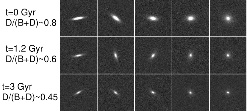
Figure 41: Examples of the artificial objects added to the $I_{\rm F814W}$-band images. The age of the toy model with $\tau=0.5$ Gyr (the disk fraction of the objects) increases (decreases) from $t=0$ Gyr (D/(B+D) $=$ 0.8) at the top row to $t=3$ Gyr (D/(B+D) $=$ 0.45) at the bottom row. The inclination angle changes from nearly edge-on view at the left column to face-on view at the right column. The three objects in the same column have the same intrinsic shape parameters for the disk and bulge components and inclination angles, but the different magnitudes of the disk and bulge components. The background sky and position angle on the image are randomly selected and different among the objects.

We here describe the Monte Carlo simulation to check how the decrease of the disk fraction due to the quenching of star formation in the disk component affects the distribution of the apparent axial ratio. Using the IRAF/ARTDATA package, we added artificial objects with disk and bulge components to sky regions at random positions in the HST/ACS $I_{\rm F814W}$-band images. Assuming these objects were located at $z=0.8$, we calculated the apparent $I_{\rm F814W}$-band magnitudes of the disk and bulge components from their absolute magnitudes of the toy model with $\tau=$ 0.5 Gyr at 0, 1.2, and 3 Gyr after the start of the disk quenching, when the disk fraction was about 0.8, 0.6, and 0.45, respectively. We assumed the exponential and de Vaucouleurs laws for surface brightness profiles of the disk and bulge components, respectively. We performed the same Monte Carlo simulations as in the fitting of the axial-ratio distribution to generate the apparent axial ratios of the disk and bulge components. In the simulations, we assumed the best-fit intrinsic shape parameters of the main-sequence and passively evolving galaxies with $M_{star}=10^{10}$–$10^{10.5}M_{\odot}$ at $0.6<z<1.0$ for the disk and bulge components, respectively, except for $\mu_{C/A}$ of the disk component, for which we adopted $\mu_{C/A}=0.18$ so that the thickness of artificial objects with the both disk and bulge components at the start of the quenching corresponds to that of the observed main-sequence galaxies. We also assumed that the major, middle, and minor axes of the disk and bulge components are aligned in the same direction for simplicity. The semi-major radii of the disk and bulge components were adjusted to match with those of the observed main-sequence and passively evolving galaxies in Figure 25. While the assumption of the size of passively evolving galaxies may overestimate that of the bulge of normal star-forming galaxies, we confirmed that smaller/larger sizes of the bulge component do not significantly change the results. We performed 10000 such simulations for each age of the toy model mentioned above, and measured the apparent axial ratios of these artificial objects with the same way as for the observed galaxies. Figure 41 shows examples of the artificial objects in the simulation.

References

- Abadi et al. (1999) Abadi, M. G., Moore, B., & Bower, R. G. 1999, MNRAS, 308, 947
- Abraham, & van den Bergh (2001) Abraham, R. G., & van den Bergh, S. 2001, Science, 293, 1273
- Aguerri (2012) Aguerri, J. A. L. 2012, Advances in Astronomy, 2012, 382674
- Barnes (1988) Barnes, J. E. 1988, ApJ, 331, 699
- Balogh et al. (2000) Balogh, M. L., Navarro, J. F., & Morris, S. L. 2000, ApJ, 540, 113
- Bell et al. (2004) Bell, E. F., Wolf, C., Meisenheimer, K., et al. 2004, ApJ, 608, 752
- Bell et al. (2007) Bell, E. F., Zheng, X. Z., Papovich, C., et al. 2007, ApJ, 663, 834
- Bell et al. (2012) Bell, E. F., van der Wel, A., Papovich, C., et al. 2012, ApJ, 753, 167
- Bertin, & Arnouts (1996) Bertin, E., & Arnouts, S. 1996, A&AS, 117, 393
- Bezanson et al. (2018) Bezanson, R., van der Wel, A., Pacifici, C., et al. 2018, ApJ, 858, 60
- Binggeli (1980) Binggeli, B. 1980, A&A, 82, 289
- Binney, & de Vaucouleurs (1981) Binney, J., & de Vaucouleurs, G. 1981, MNRAS, 194, 679
- Binney (1985) Binney, J. 1985, MNRAS, 212, 767
- Birnboim, & Dekel (2003) Birnboim, Y., & Dekel, A. 2003, MNRAS, 345, 349
- Bluck et al. (2019) Bluck, A. F. L., Bottrell, C., Teimoorinia, H., et al. 2019, MNRAS, 485, 666
- Borch et al. (2006) Borch, A., Meisenheimer, K., Bell, E. F., et al. 2006, A&A, 453, 869
- Bremer et al. (2018) Bremer, M. N., Phillipps, S., Kelvin, L. S., et al. 2018, MNRAS, 476, 12
- Bruzual, & Charlot (2003) Bruzual, G., & Charlot, S. 2003, MNRAS, 344, 1000
- Carollo et al. (2013) Carollo, C. M., Bschorr, T. J., Renzini, A., et al. 2013, ApJ, 773, 112
- Calzetti et al. (2000) Calzetti, D., Armus, L., Bohlin, R. C., et al. 2000, ApJ, 533, 682
- Capak et al. (2007) Capak, P., Aussel, H., Ajiki, M., et al. 2007, ApJS, 172, 99
- Cervantes Sodi (2017) Cervantes Sodi, B. 2017, ApJ, 835, 80
- Ceverino et al. (2010) Ceverino, D., Dekel, A., & Bournaud, F. 2010, MNRAS, 404, 2151
- Chabrier (2003) Chabrier, G. 2003, PASP, 115, 763
- Chang et al. (2013) Chang, Y.-Y., van der Wel, A., Rix, H.-W., et al. 2013, ApJ, 773, 149
- Conselice et al. (2005) Conselice, C. J., Blackburne, J. A., & Papovich, C. 2005, ApJ, 620, 564
- Darvish et al. (2017) Darvish, B., Mobasher, B., Martin, D. C., et al. 2017, ApJ, 837, 16
- Dekel, & Silk (1986) Dekel, A., & Silk, J. 1986, ApJ, 303, 39
- Dekel et al. (2009a) Dekel, A., Birnboim, Y., Engel, G., et al. 2009, Nature, 457, 451
- Dekel et al. (2009b) Dekel, A., Sari, R., & Ceverino, D. 2009, ApJ, 703, 785
- Dekel, & Burkert (2014) Dekel, A., & Burkert, A. 2014, MNRAS, 438, 1870
- Duncan et al. (2019) Duncan, K., Conselice, C. J., Mundy, C., et al. 2019, ApJ, 876, 110
- El-Badry et al. (2018) El-Badry, K., Quataert, E., Wetzel, A., et al. 2018, MNRAS, 473, 1930
- Elbaz et al. (2007) Elbaz, D., Daddi, E., Le Borgne, D., et al. 2007, A&A, 468, 33
- Emsellem et al. (2011) Emsellem, E., Cappellari, M., Krajnović, D., et al. 2011, MNRAS, 414, 888
- Faber et al. (2007) Faber, S. M., Willmer, C. N. A., Wolf, C., et al. 2007, ApJ, 665, 265
- Fabian (2012) Fabian, A. C. 2012, ARA&A, 50, 455
- Fiacconi et al. (2015) Fiacconi, D., Feldmann, R., & Mayer, L. 2015, MNRAS, 446, 1957
- Förster Schreiber et al. (2009) Förster Schreiber, N. M., Genzel, R., Bouché, N., et al. 2009, ApJ, 706, 1364
- Gehrels (1986) Gehrels, N. 1986, ApJ, 303, 336
- Governato et al. (2009) Governato, F., Brook, C. B., Brooks, A. M., et al. 2009, MNRAS, 398, 312
- Grogin et al. (2011) Grogin, N. A., Kocevski, D. D., Faber, S. M., et al. 2011, ApJS, 197, 35
- Guedes et al. (2013) Guedes, J., Mayer, L., Carollo, M., et al. 2013, ApJ, 772, 36
- Hill et al. (2019) Hill, A. R., van der Wel, A., Franx, M., et al. 2019, ApJ, 871, 76
- Holden et al. (2012) Holden, B. P., van der Wel, A., Rix, H.-W., et al. 2012, ApJ, 749, 96
- Hopkins et al. (2009) Hopkins, P. F., Somerville, R. S., Cox, T. J., et al. 2009, MNRAS, 397, 802
- Hubble (1926) Hubble, E. P. 1926, ApJ, 64, 321
- Huertas-Company et al. (2009) Huertas-Company, M., Tasca, L., Rouan, D., et al. 2009, A&A, 497, 743
- Ilbert et al. (2009) Ilbert, O., Capak, P., Salvato, M., et al. 2009, ApJ, 690, 1236
- Ilbert et al. (2010) Ilbert, O., Salvato, M., Le Floc’h, E., et al. 2010, ApJ, 709, 644
- Ilbert et al. (2013) Ilbert, O., McCracken, H. J., Le Fèvre, O., et al. 2013, A&A, 556, A55
- Ilbert et al. (2015) Ilbert, O., Arnouts, S., Le Floc’h, E., et al. 2015, A&A, 579, A2
- Jesseit et al. (2009) Jesseit, R., Cappellari, M., Naab, T., et al. 2009, MNRAS, 397, 1202
- Kajisawa, & Yamada (2001) Kajisawa, M., & Yamada, T. 2001, PASJ, 53, 833
- Kajisawa et al. (2010) Kajisawa, M., Ichikawa, T., Yamada, T., et al. 2010, ApJ, 723, 129
- Kajisawa et al. (2011) Kajisawa, M., Ichikawa, T., Yoshikawa, T., et al. 2011, PASJ, 63, 403
- Kereš et al. (2005) Kereš, D., Katz, N., Weinberg, D. H., et al. 2005, MNRAS, 363, 2
- Kereš et al. (2009) Kereš, D., Katz, N., Fardal, M., et al. 2009, MNRAS, 395, 160
- Koekemoer et al. (2007) Koekemoer, A. M., Aussel, H., Calzetti, D., et al. 2007, ApJS, 172, 196
- Koekemoer et al. (2011) Koekemoer, A. M., Faber, S. M., Ferguson, H. C., et al. 2011, ApJS, 197, 36
- Kormendy, & Kennicutt (2004) Kormendy, J., & Kennicutt, R. C. 2004, ARA&A, 42, 603
- Laigle et al. (2016) Laigle, C., McCracken, H. J., Ilbert, O., et al. 2016, ApJS, 224, 24
- Lambas et al. (1992) Lambas, D. G., Maddox, S. J., & Loveday, J. 1992, MNRAS, 258, 404
- Law et al. (2012) Law, D. R., Steidel, C. C., Shapley, A. E., et al. 2012, ApJ, 745, 85
- Larson et al. (1980) Larson, R. B., Tinsley, B. M., & Caldwell, C. N. 1980, ApJ, 237, 692
- Legrand et al. (2019) Legrand, L., McCracken, H. J., Davidzon, I., et al. 2019, MNRAS, 486, 5468
- Lotz et al. (2008) Lotz, J. M., Jonsson, P., Cox, T. J., et al. 2008, MNRAS, 391, 1137
- Mager et al. (2018) Mager, V. A., Conselice, C. J., Seibert, M., et al. 2018, ApJ, 864, 123
- Mancini et al. (2019) Mancini, C., Daddi, E., Juneau, S., et al. 2019, MNRAS, 2068
- Martig et al. (2009) Martig, M., Bournaud, F., Teyssier, R., et al. 2009, ApJ, 707, 250
- Moore et al. (1996) Moore, B., Katz, N., Lake, G., et al. 1996, Nature, 379, 613
- Morselli et al. (2019) Morselli, L., Popesso, P., Cibinel, A., et al. 2019, A&A, 626, A61
- Mundy et al. (2017) Mundy, C. J., Conselice, C. J., Duncan, K. J., et al. 2017, MNRAS, 470, 3507
- Murata et al. (2014) Murata, K. L., Kajisawa, M., Taniguchi, Y., et al. 2014, ApJ, 786, 15
- Muzzin et al. (2013) Muzzin, A., Marchesini, D., Stefanon, M., et al. 2013, ApJ, 777, 18
- Naab, & Burkert (2003) Naab, T., & Burkert, A. 2003, ApJ, 597, 893
- Noeske et al. (2007) Noeske, K. G., Weiner, B. J., Faber, S. M., et al. 2007, ApJ, 660, L43
- Noguchi (2019) Noguchi, M. 2019, arXiv e-prints, arXiv:1905.08993
- Oser et al. (2010) Oser, L., Ostriker, J. P., Naab, T., et al. 2010, ApJ, 725, 2312
- Padilla, & Strauss (2008) Padilla, N. D., & Strauss, M. A. 2008, MNRAS, 388, 1321
- Peng et al. (2010) Peng, Y.-. jie ., Lilly, S. J., Kovač, K., et al. 2010, ApJ, 721, 193
- Pillepich et al. (2019) Pillepich, A., Nelson, D., Springel, V., et al. 2019, arXiv e-prints, arXiv:1902.05553
- Popesso et al. (2019) Popesso, P., Concas, A., Morselli, L., et al. 2019, MNRAS, 483, 3213
- Qu et al. (2011) Qu, Y., Di Matteo, P., Lehnert, M. D., et al. 2011, A&A, 535, A5
- Quinn et al. (1993) Quinn, P. J., Hernquist, L., & Fullagar, D. P. 1993, ApJ, 403, 74
- Ravindranath et al. (2006) Ravindranath, S., Giavalisco, M., Ferguson, H. C., et al. 2006, ApJ, 652, 963
- Renaud et al. (2014) Renaud, F., Bournaud, F., Kraljic, K., et al. 2014, MNRAS, 442, L33
- Roberts, & Haynes (1994) Roberts, M. S., & Haynes, M. P. 1994, ARA&A, 32, 115
- Rodriguez-Gomez et al. (2017) Rodriguez-Gomez, V., Sales, L. V., Genel, S., et al. 2017, MNRAS, 467, 3083
- Roškar et al. (2008) Roškar, R., Debattista, V. P., Stinson, G. S., et al. 2008, ApJ, 675, L65
- Ryden (2004) Ryden, B. S. 2004, ApJ, 601, 214
- Sales et al. (2009) Sales, L. V., Helmi, A., Abadi, M. G., et al. 2009, MNRAS, 400, L61
- Sales et al. (2012) Sales, L. V., Navarro, J. F., Theuns, T., et al. 2012, MNRAS, 423, 1544
- Sandage et al. (1970) Sandage, A., Freeman, K. C., & Stokes, N. R. 1970, ApJ, 160, 831
- Sanders, & Mirabel (1996) Sanders, D. B., & Mirabel, I. F. 1996, ARA&A, 34, 749
- Shao et al. (2007) Shao, Z., Xiao, Q., Shen, S., et al. 2007, ApJ, 659, 1159
- Sparre, & Springel (2016) Sparre, M., & Springel, V. 2016, MNRAS, 462, 2418
- Springel, & Hernquist (2005) Springel, V., & Hernquist, L. 2005, ApJ, 622, L9
- Takeuchi et al. (2015) Takeuchi, T. M., Ohta, K., Yuma, S., et al. 2015, ApJ, 801, 2
- Taniguchi et al. (2007) Taniguchi, Y., Scoville, N., Murayama, T., et al. 2007, ApJS, 172, 9
- Taniguchi et al. (2015) Taniguchi, Y., Kajisawa, M., Kobayashi, M. A. R., et al. 2015, PASJ, 67, 104
- Teyssier et al. (2010) Teyssier, R., Chapon, D., & Bournaud, F. 2010, ApJ, 720, L149
- Tinker et al. (2013) Tinker, J. L., Leauthaud, A., Bundy, K., et al. 2013, ApJ, 778, 93
- van der Wel et al. (2009) van der Wel, A., Rix, H.-W., Holden, B. P., et al. 2009, ApJ, 706, L120
- van der Wel et al. (2014a) van der Wel, A., Chang, Y.-Y., Bell, E. F., et al. 2014, ApJ, 792, L6
- van der Wel et al. (2014b) van der Wel, A., Franx, M., van Dokkum, P. G., et al. 2014, ApJ,
- Vika et al. (2013) Vika, M., Bamford, S. P., Häußler, B., et al. 2013, MNRAS, 435, 623
- Villalobos, & Helmi (2008) Villalobos, Á., & Helmi, A. 2008, MNRAS, 391, 1806
- Vincent, & Ryden (2005) Vincent, R. A., & Ryden, B. S. 2005, ApJ, 623, 137
- Whitaker et al. (2011) Whitaker, K. E., Labbé, I., van Dokkum, P. G., et
- White, & Frenk (1991) White, S. D. M., & Frenk, C. S. 1991, ApJ, 379, 52
- Williams et al. (2009) Williams, R. J., Quadri, R. F., Franx, M., et al. 2009, ApJ, 691, 1879
- Windhorst et al. (2002) Windhorst, R. A., Taylor, V. A., Jansen, R. A., et al. 2002, ApJS, 143, 113
- Wisnioski et al. (2015) Wisnioski, E., Förster Schreiber, N. M., Wuyts, S., et al. 2015, ApJ, 799, 209
- Wuyts et al. (2012) Wuyts, S., Förster Schreiber, N. M., Genzel, R., et al. 2012, ApJ, 753, 114
- Yuma et al. (2011) Yuma, S., Ohta, K., Yabe, K., et al. 2011, ApJ, 736, 92
- Yuma et al. (2012) Yuma, S., Ohta, K., & Yabe, K. 2012, ApJ, 761, 19
- Zhang et al. (2019) Zhang, H., Primack, J. R., Faber, S. M., et al. 2019, MNRAS, 484, 5170