Transfer Learning with Dynamic Distribution Adaptation
Abstract.
Transfer learning aims to learn robust classifiers for the target domain by leveraging knowledge from a source domain. Since the source and the target domains are usually from different distributions, existing methods mainly focus on adapting the cross-domain marginal or conditional distributions. However, in real applications, the marginal and conditional distributions usually have different contributions to the domain discrepancy. Existing methods fail to quantitatively evaluate the different importance of these two distributions, which will result in unsatisfactory transfer performance. In this paper, we propose a novel concept called Dynamic Distribution Adaptation (DDA), which is capable of quantitatively evaluating the relative importance of each distribution. DDA can be easily incorporated into the framework of structural risk minimization to solve transfer learning problems. On the basis of DDA, we propose two novel learning algorithms: (1) Manifold Dynamic Distribution Adaptation (MDDA) for traditional transfer learning, and (2) Dynamic Distribution Adaptation Network (DDAN) for deep transfer learning. Extensive experiments demonstrate that MDDA and DDAN significantly improve the transfer learning performance and setup a strong baseline over the latest deep and adversarial methods on digits recognition, sentiment analysis, and image classification. More importantly, it is shown that marginal and conditional distributions have different contributions to the domain divergence, and our DDA is able to provide good quantitative evaluation of their relative importance which leads to better performance. We believe this observation can be helpful for future research in transfer learning.
1. Introduction
Supervised learning is perhaps the most popular and well-studied paradigm in machine learning during the past years. Significant advances have been achieved in supervised learning by exploiting a large amount of labeled training data to build powerful models. For instance, in computer vision, large-scale labeled datasets such as ImageNet (Deng et al., 2009) for image classification and MS COCO (Lin et al., 2014) for object detection and semantic segmentation have played an instrumental role to help train computer vision models with superior performance. In sentiment analysis, a lot of reviews for all kinds of products are available to train sentiment classification models. Unfortunately, it is often expensive and time-consuming to acquire sufficient labeled data to train these models. Furthermore, there is often dataset bias in newly emerging data, i.e. the existing model is often trained on a particular dataset and will generalize poorly in a new domain. For example, the images of an online product can be very different from those taken at home. The product review for electronic devices is likely to be different from that of clothes. Under this circumstance, it is necessary and important to design algorithms that can handle both the label scarcity and dataset bias challenges.
Domain adaptation, or transfer learning (Pan and Yang, 2010; Wang et al., 2018b) has been a promising approach to solve such problems. The main idea of transfer learning is to leverage the abundant labeled samples in some existing domains to facilitate learning in a new target domain by reducing the dataset bias. The domain with abundant labeled samples is often called the source domain, while the domain for which a new model is to be trained is the target domain. However, due to the dataset bias, the data distributions on different domains are usually different. In such circumstance, traditional machine learning algorithms cannot be applied directly since they assume that training and testing data are under the same distributions. Transfer learning is able to reduce the distribution divergence (Pan and Yang, 2010) such that the models on the target domain can be learned.
To cope with the difference in distributions between domains, existing works can be summarized into two main categories: (a) instance reweighting (Dai et al., 2007b; Xu et al., 2017), which reuses samples from the source domain according to some weighting technique; and (b) feature matching, which either performs subspace learning by exploiting the subspace geometrical structure (Wang et al., 2019; Fernando et al., 2013; Sun et al., 2016; Gong et al., 2012), or distribution alignment to reduce the marginal or conditional distribution divergence between domains (Wang et al., 2017; Zhang et al., 2017b; Long et al., 2013). Recently, the success of deep learning has dramatically increased the performance of transfer learning either via deep representation learning (Zhu et al., 2019; Yosinski et al., 2014; He et al., 2016; Bousmalis et al., 2016; Long et al., 2017; Wang et al., 2018d) or adversarial learning (Ganin et al., 2016; Ganin and Lempitsky, 2015; Long et al., 2018; Zhang et al., 2018b; Sankaranarayanan et al., 2018). The key idea behind these works is to learn more transferable representations using deep neural networks. Then, the learned feature distributions can be aligned such that their domain discrepancy can be reduced.
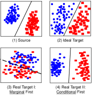
However, despite the great success achieved by traditional and deep transfer learning methods, there is still a challenge ahead. Existing works only attempt to align the marginal (Pan et al., 2011; Tzeng et al., 2014; Long et al., 2015) or the conditional distributions (Pei et al., 2018; Long et al., 2018). Although recent advance has suggested that aligning both distributions will lead to better performance (Long et al., 2013; Wang et al., 2017; Long et al., 2017), they only give the two distributions equal weights, which fails to evaluate the relative importance of these two distributions. In their assumptions, both the marginal and conditional distributions are contributing equally to the domain divergence. However, in this paper, we argue that this assumption is not practical in real applications. For example, when two domains are very dissimilar (e.g., transfer learning between (1) and (3) in Fig. 1(a)), the marginal distribution is more important. When the marginal distributions are close (transfer learning between (1) and (4) in Fig. 1(a)), the conditional distribution of each class should be given more weight. Ignoring this fact will likely to result in unsatisfactory transfer performance. There is no method which can quantitatively account for the relative importance of these two distributions in conjunction.
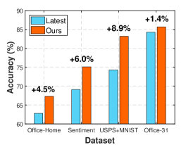
In this paper, we propose a novel concept of Dynamic Distribution Adaptation (DDA) to dynamically and quantitatively adapt the marginal and conditional distributions in transfer learning. To be specific, DDA is able to dynamically learn the distribution weights through calculating the divergence (Ben-David et al., 2007) between domains when learning representations. Then, the relative importance of marginal and conditional distributions can be obtained, which in turn can be utilized to learn more transferable feature representations. This dynamic importance learning and feature learning are being optimized iteratively to learn a domain-invariant transfer classifier eventually. To the best of our knowledge, DDA is the first work to dynamically and quantitatively evaluate the importance of both distributions. The significant improvements of DDA over the latest method on different kinds of tasks are shown in Fig. 1(b).
To enable good representation learning, we propose two novel learning methods based on DDA with the principle of Structural Risk Minimization (SRM) (Vapnik and Vapnik, 1998). For traditional transfer learning, we develop Manifold Dynamic Distribution Adaptation (MDDA) method to utilize the Grassmann manifold (Hamm and Lee, 2008) in learning non-distorted feature representations. For deep transfer learning, we develop Dynamic Distribution Adaptation Network (DDAN) to use the deep neural work in learning end-to-end transfer classifier. We also develop respective learning algorithms for MDDA and DDAN.
To sum up, this work makes the following contributions:
1) We propose the DDA concept for domain adaptation. DDA is the first quantitative evaluation framework for the relative importance of marginal and conditional distributions in domain adaptation. This is useful for a wide range of future research on transfer learning.
2) On top of DDA, we propose two novel methods: MDDA for traditional transfer learning and DDAN for deep transfer learning. Both methods can be efficiently formulated and finally learn the domain-invariant transfer classifier.
3) We conduct extensive experiments on digit classification, object recognition, and sentiment classification datasets. Experimental results demonstrate that both MDDA and DDAN are significantly better than many state-of-the-art traditional and deep methods. More importantly, empirical results have also demonstrated that the different effect of marginal and conditional distributions do exist, and our DDA is able to give them quantitative weights, which facilitates the performance of transfer learning.
This paper is an extension of our previous oral paper at ACM Multimedia conference(Wang et al., 2018c). Our extensions include: (1) A more general and clear concept of dynamic distribution adaptation and its calculation. (2) We extend DDA in both manifold learning and deep learning methods, then we formulate these algorithms and propose respective learning algorithms. (3) We extend the experiments in digit classification, sentiment analysis, and image classification, which have shown the effectiveness of our methods. And (4) We extensively analyze our calculation of DDA in new experiments.
The remainder of this paper is structured as follows. We review the related work in Section 2. In Section 3, we introduce some previous knowledge before introducing the proposed method. Section 4 thoroughly presents our proposed DDA concept and its two extensions: MDDA and DDAN. Extensive experiments are shown in Section 5, where we extensively evaluate the performance of MDDA and DDAN. Finally, Section 6 concludes this paper.
2. Related Work
Domain adaptation, or transfer learning, is an active research area in machine learning. Apart from the popular survey by Pan and Yang (Pan and Yang, 2010), several recent survey papers have extensively investigated specific research topics in transfer learning including: visual domain adaptation (Wang et al., 2018c, 2019), heterogeneous transfer learning (Day and Khoshgoftaar, 2017; Friedjungová and Jirina, 2017), multi-task learning (Zhang and Yang, 2017), and cross-dataset recognition (Zhang et al., 2017a). There are also several successful applications using transfer learning for: activity recognition (Wang et al., 2018a, d; Chen et al., 2019c, b), object recognition (Ghifary et al., 2017), face recognition (Ren et al., 2014), speech recognition (Yi et al., 2019), speech synthesis (Jia et al., 2018), and text classification (Do and Ng, 2006). Interested readers are recommended to refer to http://transferlearning.xyz to find out more related works and applications.
From the perspective of transfer learning methods, there are three main categories: (1) Instance re-weighting, which reuses samples according to some weighting technique (Dai et al., 2007b, a; Tan et al., 2015); (2) Feature transformation, which performs representation learning to transform the source and target domains into the same subspace (Long et al., 2018; Wang et al., 2017; Zhang et al., 2017b; Pan et al., 2011); (3) Transfer metric learning (Luo et al., 2018b, 2014, a), which learns transferable metric between domains. Since our proposed methods are mainly related to feature-based transfer learning, we will extensively introduce the related work in the following aspects.
2.1. Subspace and Manifold Learning
One category of feature-based transfer learning is subspace and manifold learning. The goal is to learn representative subspace or manifold representations that are invariant across domains. Along this line, subspace alignment (SA) (Fernando et al., 2013) aligned the base vectors of both domains, but failed to adapt feature distributions. Subspace distribution alignment (SDA) (Sun and Saenko, 2015) extended SA by adding subspace variance adaptation. However, SDA did not consider the local property of subspaces and ignored conditional distribution alignment. CORAL (Sun et al., 2016) aligned subspaces in second-order statistics, but it did not consider the distribution alignment. Scatter component analysis (SCA) (Ghifary et al., 2017) converted the samples into a set of subspaces (i.e. scatters) and then minimized the divergence between them.
On the other hand, some work used the property of manifold to further learn tight representations. Geodesic flow kernel (GFK) (Gong et al., 2012) extended the idea of sampled points in manifold (Gopalan et al., 2011) and proposed to learn the geodesic flow kernel between domains. The work of (Baktashmotlagh et al., 2014) used a Hellinger distance to approximate the geodesic distance in Riemann space. (Baktashmotlagh et al., 2013) proposed to use Grassmann for domain adaptation, but they ignored the conditional distribution alignment. Different from these approaches, DDA can learn a domain-invariant classifier in the manifold and align both marginal and conditional distributions.
2.2. Distribution Alignment
Another category of feature-based transfer learning is distribution alignment. The work of this category is pretty straight forward: find some feature transformations that can minimize the distribution divergence. Along this line, existing work can be classified into three subcategories: marginal distribution alignment, conditional distribution alignment, and joint distribution alignment.
DDA substantially differs from existing work that only aligns marginal or conditional distribution (Pan et al., 2011). Joint distribution adaptation (JDA) (Long et al., 2013) matched both distributions with equal weights. Others extended JDA by adding regularization (Long et al., 2014), sparse representation (Xu et al., 2016), structural consistency (Hou et al., 2016), domain invariant clustering (Tahmoresnezhad and Hashemi, 2016), and label propagation (Zhang et al., 2017b). The work of Balanced Distribution Adaptation (BDA) (Wang et al., 2017) firstly proposed to manually weight the two distributions. The main differences between DDA (MDDA) and these methods are: 1) These work treats the two distributions equally. However, when there is a greater discrepancy between both distributions, they cannot evaluate their relative importance and thus lead to undermined performance. Our work is capable of evaluating the quantitative importance of each distribution via considering their different effects. 2) These methods are designed only for the original space, where feature distortion will negatively affect the performance. DDA (MDDA) can align the distributions in the manifold to overcome the feature distortion.
2.3. Domain-invariant Classifier Learning
Different from the above two types of work that further need to learn a classifier for the target domain, some research is able to learn the domain-invariant classifier while simultaneously performing subspace learning or distribution alignment. Recent work such as adaptation regularization for transfer learning (ARTL) (Long et al., 2014), domain-invariant projection (DIP) (Baktashmotlagh et al., 2013, 2016), and distribution matching machines (DMM) (Cao et al., 2018) also aimed to build a domain-invariant classifier. However, ARTL and DMM cannot effectively handle feature distortion in the original space. Nor can they account for the different importance of distributions. DIP mainly focused on feature transformation and only aligned marginal distributions. DDA (MDDA) is able to mitigate feature distortion and quantitatively evaluate the importance of marginal and conditional distribution adaptation.
2.4. Deep and Adversarial Transfer Learning
Recent years have witnessed the advance of deep transfer learning. Compared to traditional shallow learning, deep neural networks are capable of learning better representations (Yosinski et al., 2014). Deep domain confusion (DDC) (Tzeng et al., 2014) firstly added the MMD loss to a deep network to adapt the network. Similar to DDC, deep adaptation networks (DAN) adopted the multiple-kernel MMD (Gretton et al., 2012b) to the network. Instead, Deep CORAL (Sun and Saenko, 2016) added CORAL loss (Sun et al., 2016) to the network. CORAL is a second-order loss compared to MMD, which is a first-order loss. Furthermore, Zellinger et al. introduce the central moment discrepancy (CMD) (Zellinger et al., 2017) to the network, which is a higher-order distance.
Different from the above deep transfer learning methods, adversarial learning (Goodfellow et al., 2014) also helps to learn more transferable and discriminative representations. Domain-adversarial neural network (DANN) was first introduced by Ganin et al. (Ganin and Lempitsky, 2015; Ganin et al., 2016). The core idea is to add a domain-adversarial loss to the network instead of the predefined distance function such as MMD. This has dramatically enabled the network to learn more discriminative information. Following the idea of DANN, a lot of work adopted domain-adversarial training (Long et al., 2017; Zhang et al., 2018b; Long et al., 2018; Bousmalis et al., 2016; Chen et al., 2019a).
The above-discussed work all ignore the different effect of marginal and conditional distributions in transfer learning, while our proposed DDA (DDAN) is fully capable of dynamically evaluating the importance of each distribution.
3. Preliminaries
Let be an input measurable space of dimension and the set of possible labels. We use to denote the set of all probability measures over . In standard transfer learning setting, there is a source domain with known labels and a target domain with unknown labels. Here, and are samples from either source or the target domain. Different from existing work that either assume the marginal or conditional distributions of two domains are different, in this work, we tackle a more general case that both distributions are different, i.e. . The goal is to learn a transferable classifier such that the risk on the target domain can be minimized: .
3.1. Structural Risk Minimization
From a statistical machine learning perspective, the above problem can be formulated and solved by the structural risk minimization (SRM) principle (Vapnik and Vapnik, 1998). In SRM, the prediction function can be formulated as
| (1) |
where the first term indicates the loss on data samples with is the loss function, the second term denotes the regularization term, and is the Hilbert space induced by kernel function . is the trade-off parameter. The symbol denotes the domain that has labels.
In our problem, we have since there are no labels in the target domain. Specifically, in order to effectively handle the different distributions between and , we can further divide the regularization term as
| (2) |
where represents the distribution divergence between and with the trade-off parameters and denotes other regularization.
3.2. Maximum Mean Discrepancy
There are a variety of means to measure the distribution divergence between two domains such as KullbackLeibler divergence and cross-entropy. With respect to efficiency, we adopt the maximum mean discrepancy (MMD) (Ben-David et al., 2007) to empirically calculate the distribution divergence between domains. As a non-parametric measurement, MMD has been widely adopted by many existing methods (Zhang et al., 2017b; Ghifary et al., 2017; Pan et al., 2011), and its effectiveness has been proven analytically in (Gretton et al., 2012a).
Formally, the MMD distance between distributions and is defined as (Gretton et al., 2012a)
| (3) |
where is the Reproduced kernel Hilbert space (RKHS) with Mercer kernel , is its unit norm ball, and denotes the mean of the embedded samples.
This is known as an integral probability metric in the statistics literature. To compute this divergence, a biased empirical estimate of MMD is obtained by replacing the population expectations with empirical expectations computed on the samples and ,
| (4) |
where are sample numbers of and , respectively.
4. Dynamic Distribution Adaptation
In this section, we present the general dynamic distribution adaptation framework and its two learning algorithms in detail.
4.1. The General Framework
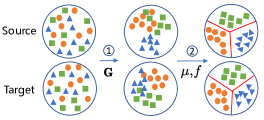
Transfer learning is to learn transferable representations which can generalize well across different domains. The key idea of Dynamic Distribution Adaptation (DDA) is to dynamically learn the relative importance of marginal and conditional distributions in transfer learning. Therefore, the dynamic importance learning and transfer feature learning are not independently, but quite involved. Accordingly, DDA first performs feature learning to learn more transferable representations. Then, it can perform dynamic distribution adaptation to quantitatively account for the relative importance of marginal and conditional distributions to address the challenge of unevaluated distribution alignment. These two steps are iteratively optimized via several iterations. Eventually, a domain-invariant classifier can be learned by combining these two steps based on the principle of SRM.
Recall the principle of SRM in Eq. (1). If we use to denote the feature learning function, then can be represented as
| (5) |
where is the squared norm of . The term represents the proposed dynamic distribution alignment. Additionally, we introduce as a Laplacian regularization to further exploit the similar geometrical property of nearest points in manifold (Belkin et al., 2006). , and are the regularization parameters.
In the next sections, we first introduce the learning of dynamic distribution adaptation. Then, we show how to learn the feature learning function either through manifold learning (i.e. Manifold Dynamic Distribution Adaptation, or MDDA in Fig. 2(a)) and deep learning (i.e. Dynamic Distribution Network, or DDAN in Fig. 2(b)).
4.2. Dynamic Distribution Adaptation
The purpose of dynamic distribution adaptation is to quantitatively evaluate the importance of aligning marginal () and conditional () distributions in domain adaptation. Existing methods (Long et al., 2013; Zhang et al., 2017b) assume that both distributions are equally important. However, this assumption may not be valid in real-world applications. For instance, when transferring from (1) to (3) in Fig. 1(a), there is a large difference between datasets. Therefore, the divergence between and is more dominant. In contrast, from (1) to (4) in Fig. 1(a), the datasets are similar. Therefore, the distribution divergence in each class ( and ) is more dominant.
In view of this phenomenon, we introduce an adaptive factor to dynamically adjust the importance of these two distributions. Formally, the dynamic distribution alignment is defined as
| (6) |
where is the adaptive factor and is the class indicator. denotes the marginal distribution alignment, and denotes the conditional distribution alignment for class .
When , it means that the distribution distance between the source and the target domains is large. Thus, marginal distribution alignment is more important ((1) (3) in Fig. 1(a)). When , it means that feature distribution between domains is relatively small, such that the distribution of each class is dominant. Thus, the conditional distribution alignment is more important ((1) (4) in Fig. 1(a)). When , both distributions are treated equally as in existing methods (Long et al., 2013; Zhang et al., 2017b). Hence, the existing methods can be regarded as special cases of the dynamic distribution alignment. By learning the optimal adaptive factor (which we will discuss later), MDDA can be applied to different domain adaptation problems.
We use the maximum mean discrepancy (MMD) (Ben-David et al., 2007) introduced in the last section to empirically calculate the distribution divergence between domains. To be specific, the marginal and conditional distribution distances can be respectively computed as
| (7) |
| (8) |
Then, DDA can be expressed as
| (9) |
Note that since has no labels, it is not feasible to evaluate the conditional distribution . Instead, we follow the idea in (Wang et al., 2017) and use the class conditional distribution to approximate . In order to evaluate , we apply prediction to using a base classifier trained on to obtain soft labels for . The soft labels may be less reliable, so we iteratively refine the prediction. Note that we only use the base classifier in the first iteration. After that, MDDA can automatically refine the labels for using results from previous iterations.
4.2.1. Quantitative Evaluation of Adaptive Factor
We can treat as a parameter and tune its value by cross-validation techniques. However, there are no labels for the target domain in unsupervised transfer learning problems. There are two indirect solutions to apply the value of in DDA rather than estimating its value: by Random guessing and by Max-min averaging. Random guessing is technically very intuitive. We can randomly pick a value of in , then perform MDDA using the corresponding to get the transfer learning result. If we repeat this process times and denote the -th transfer learning result as , then the final result can be calculated as . Max-min averaging is also simple to implement. We can search the value of in with the step of 0.1, which will generate a candidate set of : . Then, similar to random guessing, we can also obtain the averaged results as .
Although the random guessing and max-min averaging are both feasible and simple solutions to estimate , they are computationally prohibitive. More importantly, there is no guarantee of their results. It is extremely challenging to calculate the value of .
In this work, we make the first attempt towards calculating (i.e. ) by exploiting the global and local structure of domains. We adopt the -distance (Ben-David et al., 2007) as the basic measurement. The -distance is defined as the error of building a linear classifier to distinguish two domains (i.e. a binary classification). Formally, we denote the error of a linear classifier discriminating the two domains and . Then, the -distance can be defined as
| (10) |
We can directly compute the marginal -distance using the above equation, which is denoted as . For the -distance between conditional distributions, we use to denote the -distance for the th class. It can be calculated as , where and denote samples from class in and , respectively. Note that denotes the marginal difference, while denotes the conditional difference on all classes. In this paper, our assumption is that the domain divergence is caused by both the marginal and conditional distributions. Therefore, can represent the whole divergence. Eventually, can be estimated as
| (11) |
Note that the number of labeled samples in the source domain is often much larger than that in the target domain. Therefore, in order to solve this imbalanced classification problem, we perform upsampling (Krawczyk, 2016) on the target domain to make the samples with almost the same size. We also notice that this upsampling process is random, thus we repeat this step several times to get the averaged value.
This estimation has to be computed during every iteration of the dynamic distribution adaptation, since the feature distribution may vary after evaluating the conditional distribution each time. To the best of our knowledge, this is the first solution to quantitatively estimate the relative importance of each distribution. In fact, this estimation can be significant for future research in transfer learning and domain adaptation.
Remark: Currently, the quantitative evaluation of only supports the situation where the label space of the source and the target domains are the same. However, it is important to note that this evaluation is also open for open set domain adaptation (Panareda Busto and Gall, 2017) or partial transfer learning (Zhang et al., 2018a), where the label spaces are not the same. In such cases, we should consider the different similarity between each class in two domains. For instance, we can regard the classes that do not belong to the target domain as outliers and perform outlier detection before calculating . Then, we can select the most similar samples and classes in both domains and perform DDA. We leave this part for future research.
4.3. MDDA: Manifold Dynamic Distribution Adaptation
In this section, we introduce the learning of DDA through manifold learning. We propose Manifold Dynamic Distribution Adaptation (MDDA) as shown in Fig. 2(a). Manifold feature learning can serve as the feature learning step to mitigate the influence of feature distortion (Baktashmotlagh et al., 2013) in transfer learning. The features in manifold space can reflect a more detailed structure and property of the domains, thus avoiding feature distortion. MDDA learns in the Grassmann manifold (Hamm and Lee, 2008) since features in the manifold have some geometrical structures (Belkin et al., 2006; Hamm and Lee, 2008) that can avoid distortion in the original space. In addition, can facilitate classifier learning by treating the original -dimensional subspace (i.e. feature vector) as its basic elements. Feature transformation and distribution alignment often have efficient numerical forms (i.e., they can be represented as matrix operations easily) and facilitate domain adaptation on (Hamm and Lee, 2008). There are several approaches to transform the features into (Gopalan et al., 2011; Baktashmotlagh et al., 2014). We embed Geodesic Flow Kernel (GFK) (Gong et al., 2012) to learn for its computational efficiency.
When learning manifold features, MDDA tries to model the domains with -dimensional subspaces and then embed them into . Let and denote the PCA subspaces for the source and the target domain, respectively. can thus be regarded as a collection of all -dimensional subspaces. Each original subspace can be seen as a point in . Therefore, the geodesic flow between two points can be used to establish a path between the two subspaces, where denotes the calculus variant between two domains. If we let and , then finding a geodesic flow from to equals to transforming the original features into an infinite-dimensional feature space, which eventually eliminates the domain shift. This approach can be seen as an incremental way of ‘walking’ from to . Specifically, the new features can be represented as . From (Gong et al., 2012), the inner product of transformed features and gives rise to a positive semidefinite geodesic flow kernel
| (12) |
The geodesic flow can be parameterized as
| (13) |
where presents the orthogonal complements to . and are two orthonormal matrices that can be computed by singular value decomposition (SVD)
| (14) |
According to GFK (Gong et al., 2012), the geodesic flow kernel can be calculated by
| (15) |
where are three diagonal matrices with elements
| (16) |
Thus, the features in the original space can be transformed into Grassmann manifold with .
After manifold feature learning and dynamic distribution alignment, can be learned by summarizing SRM over and distribution alignment. By adopting the square loss , can be expressed as
| (17) |
In order to perform efficient learning, we now further reformulate each term.
SRM on the Source Domain: Using the representer theorem (Belkin et al., 2006), can be expanded as
| (18) |
where is the coefficients vector and is a kernel. Then, SRM on becomes
| (19) |
where is the Frobenious norm. is the kernel matrix with , and is a diagonal domain indicator matrix with if , otherwise . is the label matrix from the source and the target domains. denotes the trace operation. is the shrinkage parameter. Although the labels for are unavailable, they can be filtered out by the indicator matrix .
Dynamic distribution adaptation: Using the representer theorem and kernel tricks, dynamic distribution alignment in equation (9) becomes
| (20) |
where is the MMD matrix with its element calculated by
| (21) |
| (22) |
where and .
Laplacian Regularization: Additionally, we add a Laplacian regularization term to further exploit the similar geometrical property of nearest points in manifold (Belkin et al., 2006). We denote the pair-wise affinity matrix as
| (23) |
where is a similarity function (such as cosine distance) for measuring the distance between two points. denotes the set of -nearest neighbors to point . is a free parameter and must be set in the method. By introducing Laplacian matrix with diagonal matrix , the final regularization can be expressed as
| (24) |
Overall Reformulation: By combining equations (19), (20) and (24), in equation (17) can be reformulated as
| (25) |
Setting derivative , we obtain the solution
| (26) |
4.4. DDAN: Dynamic Distribution Adaptation Network
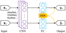
In this section, we propose Dynamic Distribution Adaptation Network (DDAN) to perform end-to-end learning of not only the feature learning function , but the classifier . DDAN is able to leverage the ability of the recent advance of deep neural networks in learning representative features through end-to-end training (Bengio et al., 2013). Specifically, we exploit a backbone network to learn useful feature representations, while simultaneously performing domain adaptation using DDA.
The network architecture of DDAN is shown in Fig 2(b). Firstly, the samples from the source and target domains serve as the inputs into the deep neural networks. Secondly, the CNN network (the purple part) such as AlexNet (Krizhevsky et al., 2012) and ResNet (He et al., 2016) can extract high-level features from the inputs. Thirdly, the features are going through a fully-connected layer (the blue part) to perform soft-max classification to obtain the labels . The novel contribution here is to align the source and target domain features using the dynamic distribution alignment (DDA, the yellow part).
Adopting the DDA, the learning objective of DDAN can be expressed as
| (27) |
where is the cross-entropy loss function and containing the weight and bias parameters of the neural network. Note that DDAN is based on the deep neural network, so instead of using the whole domain data, we use the batch data by following the mini-batch stochastic gradient descent (SGD) training procedure. Therefore, the dynamic distribution adaptation is only calculated between batches rather than whole domains. This is more practical and efficient in real applications where the data are coming in a streaming manner.
Most MMD based deep transfer learning methods (Tzeng et al., 2014) are based on Eq. (4) and only adopted the linear kernel for simplicity. Since the formulation in Eq. (4) is based on pairwise similarity and is computed in quadratic time complexity, it is prohibitively time-consuming for using mini-batch stochastic gradient decent (SGD) in CNN-based transfer learning methods. Gretton et al. (Gretton et al., 2012b) further suggest an unbiased approximation of MMD with linear complexity. Without loss of generality, by assuming , MMD can then be computed as
| (28) |
where is an operator defined on a quad-tuple ,
| (29) |
The approximation in Eq. 28 takes a summation form and is suitable for gradient computation in a mini-batch manner.
The gradient of the parameters can be computed as:
| (30) |
Updating : Another important aspect is to dynamically update in DDAN. Similar to the above mini-batch learning of MMD distance, it seems natural to calculate after each mini-batch learning. However, the labels on the source domain and the pseudo labels on the target domain are likely to be inconsistent after mini-batch learning. For instance, assume that the batch size for both domains is and the total class number . Then, after a forward operation for one batch, we can obtain 32 pseudo labels for the target domain. Since is rather close to , it is highly likely that the mini-batch labels for both domains do not match, which will easily lead to the mode collapse or gradient exploding problem.
In order to avoid this problem, we propose to update after each epoch of iteration, rather than each mini-batch data. In fact, this step is very similar to that of MDDA, which uses all the data to perform learning. The learning process of DDAN is summarized in Algorithm 2.
4.5. Discussions
Both MDDA and DDAN are generic learning methods that are suitable for all transfer classification problems. In this section, we briefly discuss their differences.
MDDA is for traditional learning, while DDAN is for deep learning. Compared to DDAN which is designed for deep neural networks, MDDA can be easily applied on the small resource constraint devices. One possible limitation of MDDA maybe that it relies on certain feature extraction methods. For instance, on image dataset, we probably need to extract SIFT, SURF, or HOG features. Luckily, MDDA can also use the deep features extracted by deep neural networks such as AlexNet (Krizhevsky et al., 2012) and ResNet (He et al., 2016). MDDA has a very useful property: it can learn the cross-domain function directly without the need for explicit classifier training. This makes it significantly more advantageous compared to most existing work such as JGSA (Zhang et al., 2017b) and SCA (Ghifary et al., 2017) which needs to train an extra classifier after learning transferrable features.
On the other hand, DDAN is suitable for cloud computing. The model of DDAN can be trained in an end-to-end manner and then be used for inference on the device. DDAN does not need extra feature extraction and classifier training procedure. All steps can be unified in one single deep neural network. This advantage makes it useful for large-scale datasets, which will probably result in prohibitive computations for MDDA.
5. Experiments and Evaluations
In this section, we evaluate the performance of MDDA through extensive experiments on large-scale public datasets. The source code for MDDA is available at http://transferlearning.xyz. We will focus on evaluating the performance of MDDA since most of our contributions can be covered by MDDA. In the last part of this section, we will evaluate the performance of the deep version of MDDA.
5.1. Experimental Setup
5.1.1. Datasets
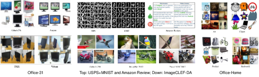
We adopted five public image datasets: USPS+MNIST, Amazon review (Blitzer et al., 2006), Office-31 (Saenko et al., 2010), ImageCLEF-DA (Long et al., 2017), and Office-Home (Venkateswara et al., 2017). These datasets are popular for benchmarking domain adaptation algorithms and have been widely adopted in most existing work such as (Zhang et al., 2017b; Long et al., 2018; Zhang et al., 2018b; Chen et al., 2019a). Fig. 3 shows some samples of the datasets, and Table 1 lists their statistics.
| Dataset | #Sample | #Feature for MDDA | #Class | Domain | Type |
|---|---|---|---|---|---|
| USPS+MNIST | 3,800 | 256 | 10 | U, M | Digit |
| Amazon review | 1,123 | 400 | 2 | B, D, E, K | Text |
| Office-31 | 4,110 | 2,048 | 31 | A, W, D | Image |
| ImageCLEF DA | 1,800 | 2,048 | 12 | C, I, P | Image |
| Office-Home | 15,500 | 2,048 | 65 | Ar, Cl, Pr, Rw | Image |
USPS (U) and MNIST (M) are standard digit recognition datasets containing handwritten digits from 0-9. Since the same digits across two datasets follow different distributions, it is necessary to perform domain adaptation. USPS consists of 7,291 training images and 2,007 test images of size 16 16. MNIST consists of 60,000 training images and 10,000 test images of size 28 28. We construct two tasks: U M and M U. In the rest of the paper, we use to denote the knowledge transfer from source domain A to the target domain B.
Amazon review (Blitzer et al., 2006) is the benchmark dataset for cross-domain sentiment analysis. This dataset includes reviews about the Kitchen appliances (K), DVDs (D), Books (B) and Electronics (E). The reviews of each product can be regarded as data from the same domain. There are 1000 positive and 1000 negative instances on each domain. Transfer learning can be conducted between any two domains, leading to 12 tasks.
Office-31 (Saenko et al., 2010) consists of three real-world object domains: Amazon (A), Webcam (W) and DSLR (D). It has 4,652 images with 31 categories. Caltech-256 (C) contains 30,607 images and 256 categories. We constructed 6 tasks: A D, A W, D A, D W, W A, W D.
ImageCLEF-DA (Long et al., 2017) is a dataset presented in the ImageCLEF 2014 domain adaptation challenge. It is composed by selecting the 12 common classes shared by three public datasets (domains): Caltech-256 (C), ImageNet ILSVRC 2012 (I), and Pascal VOC 2012 (P). There are 50 images in each category and 600 images in each domain, while Office-31 has different domain sizes. We permute domains and build 6 transfer tasks: C I, C P, I C, I P, P C, P I.
Office-Home (Venkateswara et al., 2017) is a new dataset which consists of 15,588 images from 4 different domains: Artistic images (Ar), Clip Art (Cl), Product images (Pr), and Real-World images (Rw). For each domain, the dataset contains images of 65 object categories collected from office and home settings. We use all domains and construct 12 transfer learning tasks: Ar Cl, , Rw Pr.
In total, we constructed tasks.
5.1.2. State-of-the-art Comparison Methods
We compared the performance of MDDA with several state-of-the-art traditional and deep transfer learning approaches.
Traditional transfer learning methods:
-
•
NN, SVM, and PCA
-
•
TCA: Transfer Component Analysis (Pan et al., 2011), which performs marginal distribution alignment
-
•
GFK: Geodesic Flow Kernel (Gong et al., 2012), which performs manifold feature learning
-
•
JDA: Joint Distribution Adaptation (Long et al., 2013), which adapts marginal & conditional distribution
-
•
CORAL: CORrelation Alignment (Sun et al., 2016), which performs second-order subspace alignment
-
•
SCA: Scatter Component Analysis (Ghifary et al., 2017), which adapts scatters in subspace
-
•
JGSA: Joint Geometrical and Statistical Alignment (Zhang et al., 2017b), which aligns marginal & conditional distributions with label propagation
Deep transfer learning methods:
- •
-
•
DDC: Deep Domain Confusion (Tzeng et al., 2014), which is a single-layer deep adaptation method
-
•
DAN: Deep Adaptation Network (Long et al., 2015), which is a multi-layer adaptation method
-
•
DANN: Domain Adversarial Neural Network (Ganin and Lempitsky, 2015), which is a adversarial deep neural network
-
•
ADDA: Adversarial Discriminative Domain Adaptation (Tzeng et al., 2017), which is a general framework for adversarial transfer learning
-
•
JAN: Joint Adaptation Networks (Long et al., 2017), which is a deep network with joint MMD distance
-
•
CAN: Collaborative and Adversarial Network (Zhang et al., 2018b), which is based on joint training
-
•
CDAN: Conditional Domain Adversarial Networks (Long et al., 2018), which is a conditional network
5.1.3. Implementation Details
MDDA requires to extract features from the raw inputs. For USPS+MNIST datasets, we adopted the 256 SURF features by following existing work (Zhang et al., 2017b; Wang et al., 2017). For Amazon review dataset, we follow the feature generation method to exploit marginalized denoising autoencoders (Chen et al., 2012) to improve the feature representations. For Office-31, ImageCLEF DA, and Office-Home datasets, we adopted the 2048 fine-tuned ResNet-50 features for a fair comparison. As for DDAN, we only report its results on three image datasets since USPS+MNIST and Amazon review datasets are rather simple to transfer. DDAN is able to take the original image data as inputs. We also adopted ResNet-50 as the baseline network for fair comparison (Zhang et al., 2018b; Long et al., 2018).
For the comparison methods, we either cite the results reported in their original papers or run experiments using their publicly available codes. As for MDDA, we set the manifold feature dimension for the five datasets, respectively. The number of iteration is set to . We use the RBF kernel with the bandwidth set to be the variance of inputs. The regularization parameters are set as , and . Additionally, the experiments on parameter sensitivity and convergence analysis in Section 5.5 indicate that the performance of MDDA and DDAN stays robust with a wide range of parameter choices. For DDAN, we set the learning rate to be 0.01 with the batch size to be 32 and a weight decay of . Other parameters are tuned by following transfer cross validation (Zhong et al., 2009).
Although MDDA is easy to use, and its parameters do not have to be fine-tuned. For research purpose, we also investigate how to further tune those parameters. We choose parameters according to the following rules. Firstly, SRM on source domain is very important. Thus, we prefer a small to make sure MDDA does not degenerate. Secondly, distribution alignment is required by SRM. Thus, we choose a slightly larger to make it effective. Thirdly, we choose by following the existing work (Belkin et al., 2006). Fourthly, is set following (Cai et al., 2011).
5.2. Results and Analysis
5.2.1. Results on Digit Datasets
The classification results on USPS+MNIST datasets are shown in Table 2. On the digit recognition tasks, MDDA outperforms the best method JGSA by a large margin of . These results clearly indicate that MDDA significantly outperforms existing methods.
Moreover, the performances of distribution alignment methods (TCA, JDA, and JGSA) and subspace learning methods (GFK, CORAL, and SCA) were generally inferior to MDDA. Each method has its limitations and cannot handle domain adaptation in specific tasks, especially with degenerated feature transformation and unevaluated distribution alignment. After manifold or subsapce learning, there still exists large domain shift (Baktashmotlagh et al., 2013); while feature distortion will undermine the distribution alignment methods.
| Task | 1NN | SVM | TCA | GFK | JDA | CORAL | SCA | JGSA | MDDA |
| U M | 44.7 | 62.2 | 51.2 | 46.5 | 59.7 | 30.5 | 48.0 | 68.2 | 76.8 |
| M U | 65.9 | 68.2 | 56.3 | 61.2 | 67.3 | 49.2 | 65.1 | 80.4 | 89.6 |
| AVG | 55.3 | 65.2 | 53.8 | 53.9 | 63.5 | 39.9 | 56.6 | 74.3 | 83.2 |
5.2.2. Results on Sentiment Analysis Dataset
The results on Amazon review datasets are shown in Table 3. From the results, we can observe that our proposed MDDA outperforms the best baseline method CORAL by a large margin of 6.0%. This clearly indicated that MDDA is able to dramatically reduce the divergence between different text domains.
| Method | 1NN | TCA | GFK | SA | JDA | CORAL | JGSA | MDDA |
| B D | 49.6 | 63.6 | 66.4 | 67.0 | 64.2 | 71.6 | 66.6 | 77.8 |
| B E | 49.8 | 60.9 | 65.5 | 70.8 | 62.1 | 65.1 | 75.0 | 80.0 |
| B K | 50.3 | 64.2 | 69.2 | 72.2 | 65.4 | 67.3 | 72.1 | 79.9 |
| D B | 53.3 | 63.3 | 66.3 | 67.5 | 62.4 | 70.1 | 55.5 | 74.7 |
| D E | 51.0 | 64.2 | 63.7 | 67.1 | 66.3 | 65.6 | 67.3 | 80.4 |
| D K | 53.1 | 69.1 | 67.7 | 69.4 | 68.9 | 67.1 | 65.6 | 81.0 |
| E B | 50.8 | 59.5 | 62.4 | 61.4 | 59.2 | 67.1 | 51.6 | 63.8 |
| E D | 50.9 | 62.1 | 63.4 | 64.9 | 61.6 | 66.2 | 50.8 | 62.5 |
| E K | 51.2 | 74.8 | 73.8 | 70.4 | 74.7 | 77.6 | 55.0 | 84.4 |
| K B | 52.2 | 64.1 | 65.5 | 64.4 | 62.7 | 68.2 | 58.3 | 63.5 |
| K D | 51.2 | 65.4 | 65.0 | 64.6 | 64.3 | 68.9 | 56.4 | 72.2 |
| K E | 52.3 | 74.5 | 73.0 | 68.2 | 74.0 | 75.4 | 51.7 | 80.7 |
| AVG | 51.3 | 65.5 | 66.8 | 67.3 | 65.5 | 69.1 | 60.5 | 75.1 |
5.2.3. Results on Image Datasets
The classification accuracy results on the Office-31, ImageCLEF DA, and Office-Home datasets are shown in Tables 4, 5, and 6, respectively. From those results, we can make the following observations.
Firstly, MDDA outperforms all other traditional and deep comparison methods in most tasks (20/24 tasks). The average classification accuracy achieved by MDDA on all the image tasks is %. Specifically, on the hardest Office-Home dataset, MDDA significantly outperforms the latest deep transfer learning method CDAN (Long et al., 2018) by , which clearly demonstrates the effectiveness of MDDA. The results indicates that MDDA is capable of significantly reducing the distribution divergence in domain adaptation problems.
Secondly, DDAN also substantially outperforms all the traditional and deep methods on most tasks. Note that DDAN is only based on deep neural network without adversarial training, while other deep methods such as CAN (Zhang et al., 2018b) and CDAN (Long et al., 2018) all require to train an adversarial neural network, which clearly needs more time to converge. In this way, DDAN is much more efficient than these networks.
Thirdly, we also note that traditional methods such as TCA, JDA, and CORAL can also achieve good performance compared to ResNet, 1NN, and SVM. This clearly indicates the necessity of transfer learning when building models from two domains. Again, our proposed MDDA and DDAN can achieve the best performances.
| Method | Baseline | Traditional transfer learning | Deep transfer learning | DDA | |||||||||||
| Task | ResNet | 1NN | SVM | TCA | GFK | JDA | CORAL | DDC | DAN | DANN | ADDA | JAN | CAN | MDDA | DDAN |
| A D | 68.9 | 79.1 | 76.9 | 74.1 | 77.9 | 80.7 | 81.5 | 76.5 | 78.6 | 79.7 | 77.8 | 84.7 | 85.5 | 86.3 | 84.9 |
| A W | 68.4 | 75.8 | 73.3 | 72.7 | 72.6 | 73.6 | 77.0 | 75.6 | 80.5 | 82.0 | 86.2 | 85.4 | 81.5 | 86.0 | 88.8 |
| D A | 62.5 | 60.2 | 64.1 | 61.7 | 62.3 | 64.7 | 65.9 | 62.2 | 63.6 | 68.2 | 69.5 | 68.6 | 65.9 | 72.1 | 65.3 |
| D W | 96.7 | 96.0 | 96.5 | 96.7 | 95.6 | 96.5 | 97.1 | 96.0 | 97.1 | 96.9 | 96.2 | 97.4 | 98.2 | 97.1 | 96.7 |
| W A | 60.7 | 59.9 | 64.9 | 60.9 | 62.8 | 63.1 | 64.3 | 61.5 | 62.8 | 67.4 | 68.9 | 70.0 | 63.4 | 73.2 | 65.0 |
| W D | 99.3 | 99.4 | 99.0 | 99.6 | 99.0 | 98.6 | 99.6 | 98.2 | 99.6 | 99.1 | 98.4 | 99.8 | 99.7 | 99.2 | 100 |
| AVG | 76.1 | 78.4 | 79.1 | 77.6 | 78.4 | 79.5 | 80.9 | 78.3 | 80.4 | 82.2 | 82.9 | 84.3 | 82.4 | 85.7 | 83.5 |
| Method | Baseline | Traditional transfer learning | Deep transfer learning | DDA | ||||||||||
| Task | ResNet | 1NN | SVM | TCA | GFK | JDA | CORAL | DAN | DANN | JAN | CAN | CDAN | MDDA | DDAN |
| C I | 78.0 | 83.5 | 86.0 | 89.3 | 86.3 | 90.8 | 83.0 | 86.3 | 87.0 | 89.5 | 89.5 | 91.2 | 92.0 | 91.0 |
| C P | 65.5 | 71.3 | 73.2 | 74.5 | 73.3 | 73.6 | 71.5 | 69.2 | 74.3 | 74.2 | 75.8 | 77.2 | 78.8 | 76.0 |
| I C | 91.5 | 89.0 | 91.2 | 93.2 | 93.0 | 94.0 | 88.7 | 92.8 | 96.2 | 94.7 | 94.2 | 96.7 | 95.7 | 94.0 |
| I P | 74.8 | 74.8 | 76.8 | 77.5 | 75.5 | 75.3 | 73.7 | 74.5 | 75.0 | 76.8 | 78.2 | 78.3 | 79.8 | 78.0 |
| P C | 91.2 | 76.2 | 85.8 | 83.7 | 82.3 | 83.5 | 72.0 | 89.8 | 91.5 | 91.7 | 89.2 | 93.7 | 95.5 | 92.7 |
| P I | 83.9 | 74.0 | 80.2 | 80.8 | 78.0 | 77.8 | 71.3 | 82.2 | 86.0 | 88.0 | 87.5 | 91.2 | 91.5 | 91.0 |
| AVG | 80.7 | 78.1 | 82.2 | 83.2 | 81.4 | 82.5 | 76.7 | 82.5 | 85.0 | 85.8 | 85.7 | 88.1 | 88.9 | 87.2 |
| Method | Baseline | Traditional transfer learning | Deep transfer learning | DDA | |||||||||
| Task | ResNet | 1NN | SVM | TCA | GFK | JDA | CORAL | DAN | DANN | JAN | CDAN | MDDA | DDAN |
| Ar Cl | 34.9 | 45.3 | 45.3 | 38.3 | 38.9 | 38.9 | 42.2 | 43.6 | 45.6 | 45.9 | 46.6 | 54.9 | 51.0 |
| Ar Pr | 50.0 | 60.1 | 65.4 | 58.7 | 57.1 | 54.8 | 59.1 | 57.0 | 59.3 | 61.2 | 65.9 | 75.9 | 66.0 |
| Ar Rw | 58.0 | 65.8 | 73.1 | 61.7 | 60.1 | 58.2 | 64.9 | 67.9 | 70.1 | 68.9 | 73.4 | 77.2 | 73.9 |
| Cl Ar | 37.4 | 45.7 | 43.6 | 39.3 | 38.7 | 36.2 | 46.4 | 45.8 | 47.0 | 50.4 | 55.7 | 58.1 | 57.0 |
| Cl Pr | 41.9 | 57.0 | 57.3 | 52.4 | 53.1 | 53.1 | 56.3 | 56.5 | 58.5 | 59.7 | 62.7 | 73.3 | 63.1 |
| Cl Rw | 46.2 | 58.7 | 60.2 | 56.0 | 55.5 | 50.2 | 58.3 | 60.4 | 60.9 | 61.0 | 64.2 | 71.5 | 65.1 |
| Pr Ar | 38.5 | 48.1 | 46.8 | 42.6 | 42.2 | 42.1 | 45.4 | 44.0 | 46.1 | 45.8 | 51.8 | 59.0 | 52.0 |
| Pr Cl | 31.2 | 42.9 | 39.1 | 37.5 | 37.6 | 38.2 | 41.2 | 43.6 | 43.7 | 43.4 | 49.1 | 52.6 | 48.4 |
| Pr Rw | 60.4 | 68.9 | 69.2 | 64.1 | 64.6 | 63.1 | 68.5 | 67.7 | 68.5 | 70.3 | 74.5 | 77.8 | 72.7 |
| Rw Ar | 53.9 | 60.8 | 61.1 | 52.6 | 53.8 | 50.2 | 60.1 | 63.1 | 63.2 | 63.9 | 68.2 | 67.9 | 65.1 |
| Rw Cl | 41.2 | 48.3 | 45.6 | 41.7 | 42.3 | 44.0 | 48.2 | 51.5 | 51.8 | 52.4 | 56.9 | 57.6 | 56.6 |
| Rw Pr | 59.9 | 74.7 | 75.9 | 70.5 | 70.6 | 68.2 | 73.1 | 74.3 | 76.8 | 76.8 | 80.7 | 81.8 | 78.9 |
| Avg | 46.1 | 56.4 | 56.9 | 51.3 | 51.2 | 49.8 | 55.3 | 56.3 | 57.6 | 58.3 | 62.8 | 67.3 | 62.5 |
5.3. Evaluation of Dynamic Distribution Adaptation
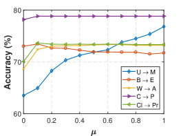

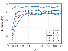
We verify the effectiveness of dynamic distribution adaptation in this section. We answer two important questions: 1) Does the different effect of marginal and conditional distributions exist in transfer learning? And 2) Is our evaluation algorithm for DDA effective? It is worth noting that there is no ground-truth for . Therefore, in order to verify our evaluation, we record the performance of DDA by searching different values. The hint is that better value contributes better performance. Specifically, we run DDA by searching . To answer the first question, we draw the results of DDA under different values of in Fig. 4(a). To answer the second question, we compare the error made by random search (Random), average search (Average), and our evaluation in Fig. 4(b).
Firstly, it is clear that the classification accuracy varies with different choices of . This indicates the necessity to consider the different effects between marginal and conditional distributions. We can also observe that the optimal value varies on different tasks ( for the three tasks, respectively). Thus, it is necessary to dynamically adjust the distribution alignment between domains according to different tasks. Moreover, the optimal value of is not unique for a given task. The classification results may be the same even for different values of .
Secondly, we also report the results of our evaluation and average search in Table 7. Combining the results in Fig. 4(b), we can conclude that our evaluation of is significantly better than random search and average search. Additionally, both random search and average search require to run the whole MDDA or DDAN algorithm several times to get steady results, our evaluation is only required once in each iteration of the algorithm. This means that our evaluation is more efficient. It is worth noting that our evaluation is extremely close to the results from grid search. Note that on task M U of Table 7, our evaluation exceeds the results of grid search. Considering that there is often few or none labels in the target domain, grid search is not actually possible. Therefore, our evaluation of can be used to approximate the ground truth in real applications.
Thirdly, we noticed that on image classification datasets, the performance of MDDA is slightly better than DDAN. MDDA is a shallow learning method, which is much easier to tune hyperparameters than DDAN, which is based on deep learning. We think that after a more extensive hyperparameter tuning process, the performance of DDAN will be the same or better as MDDA.
| Task | M U | B E | E D | A W | W A | C P | P C | Ar Rw | Cl Pr | Rw Cl | AVG |
|---|---|---|---|---|---|---|---|---|---|---|---|
| AVSE | -11.83 | -1.95 | -1.40 | -4.03 | -4.69 | -0.66 | -0.67 | -1.49 | -3.56 | -1.21 | -3.15 |
| Ours | +0.22 | -1.25 | -0.80 | -1.26 | -0.14 | -0.00 | -0.00 | -0.02 | -0.29 | -0.02 | -0.37 |
5.4. Ablation Study
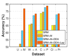
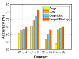
In this section, we conduct ablation study of MDDA and DDAN. MDDA mainly consists of four components: SRM, manifold learning, DDA, and Laplacian regularization. DDAN is composed of a deep network, DDA, and Laplacian regularization. We extensively analyze the performance of MDDA and DDAN on some tasks from each dataset and present the results in Fig. 5.
The results clearly indicate that each component is important to DDA. Of all the components, it is shown that our proposed DDA component is the most important part, which dramatically increases the results of transfer learning. For MDDA, manifold feature learning shows marginal improvement, while it could help to eliminate the feature distortion of the original space (Baktashmotlagh et al., 2013). For DDAN, we can clearly see that our DDA component is better than DAN, which is only adapting the marginal distributions. This again clarifies the importance of the proposed DDA framework. Finally, It seems that Laplacian regularization also generates marginal improvements except on the digit datasets (USPS+MNIST). We add Laplacian regularization since it helps the algorithm to converge quickly.
5.5. Parameter Sensitivity and Convergence Analysis
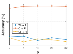
As with other state-of-the-art domain adaptation algorithms (Zhang et al., 2017b; Long et al., 2014; Ghifary et al., 2017), MDDA and DDAN also involve several parameters. In this section, we evaluate the parameter sensitivity of them. Experimental results demonstrated the robustness of MDDA and DDAN under a wide range of parameter choices.
| Task | ARTL | JGSA | DANN | CDAN | MDDA | DDAN |
|---|---|---|---|---|---|---|
| U M | 29.1 | 14.6 | - | - | 31.4 | - |
| B E | 22.8 | 18.7 | - | - | 23.5 | - |
| W A | 45.6+763.6 | 66.5 + 763.6 | 1567.3 | 1873.2 | 48.8 + 7663.6 | 1324.1 |
| C P | 124.2 + 1321.4 | 198.3 + 1321.4 | 2342.1 | 2451.2 | 156.7 + 1321.4 | 2109.8 |
| Cl Pr | 187.4 + 1768.7 | 244.3 + 1768.7 | 2877.7 | 2956.5 | 207.4 + 1768.7 | 2698.1 |
5.5.1. MDDA
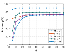
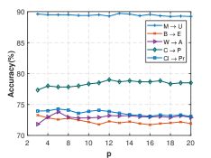
We investigated the sensitivity against manifold subspace dimension and #neighbor through experiments with a wide range of and on randomly selected tasks. From the results in Fig. 6(a) and 6(b), it can be observed that MDDA is robust with regard to different values of and . Therefore, they can be selected without in-depth knowledge of specific applications.
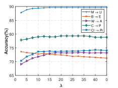
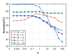
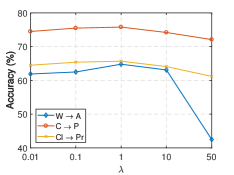
We ran MDDA with a wide range of values for regularization parameters , and on several random tasks and compare its performance with the best baseline method. We only report the results of in Fig. 6(c), and the results of and are following the same tendency. We observed that MDDA can achieve a robust performance with regard to a wide range of parameter values. Specifically, the best choices of these parameters are: , and .
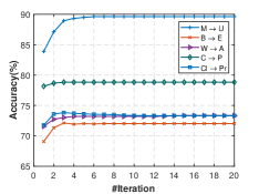
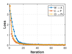
We evaluate the convergence of MDDA through experimental analysis. From the results in Fig. 6(f), it can be observed that MDDA can reach a steady performance in only a few iterations. It indicates the training advantage of MDDA in cross-domain tasks.
5.5.2. DDAN
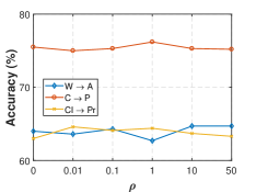
DDAN involves three key parameters: and . Similar to MDDA, we report the parameter sensitivity and convergence in Fig. 7. It is clear that DDAN is robust to these parameters. Therefore, in real applications, the hyperparameters of DDAN do not have to be cherry-picked. This is extremely important in deep learning since it is rather time-consuming to tune the hyperparameters.
We also extensively evaluate the convergence of DDAN in Fig. 7(d). It is shown that DDAN is able to converge quickly with steady performance.
5.5.3. Time complexity
We empirically check the running time of MDDA and DDAN, and present the results in Table 8. Note that for image classification tasks, the running time of ARTL, JGSA, and MDDA are the summation of deep feature extraction and algorithm running time, since these algorithms require to extract features before transfer learning. It is shown that both MDDA and DDAN can achieve efficient computing time while achieving better performance compared to these comparison methods.
6. Conclusions and Future Work
In this paper, to solve the transfer learning problem, we propose the novel dynamic distribution adaptation (DDA) concept. DDA is able to dynamically evaluate the relative importance between the source and target domains. Based on DDA, we propose two novel methods: the manifold DDA (MDDA) for traditional transfer learning, and deep DDA networks (DDAN) for deep transfer learning. Extensive experiments on digit recognition, sentiment analysis, and image classification have demonstrated that both MDDA and DDAN could achieve the best performance compared to other state-of-the-art traditional and deep transfer learning methods.
In the future, we plan to extend the DDA framework into the heterogeneous transfer learning areas as well as apply it to more complex transfer learning situations.
Acknowledgments
This work is supported in part by National Key R & D Program of China (2016YFB1001200), NSFC (61572471, 61972383), the support of grants from Hong Kong CERG projects 16209715, 16244616, Nanyang Technological University, Nanyang Assistant Professorship (NAP), and Beijing Municipal Science & Technology Commission (Z171100000117017).
References
- (1)
- Baktashmotlagh et al. (2016) Mahsa Baktashmotlagh, Mehrtash Harandi, and Mathieu Salzmann. 2016. Distribution-matching embedding for visual domain adaptation. The Journal of Machine Learning Research 17, 1 (2016), 3760–3789.
- Baktashmotlagh et al. (2013) Mahsa Baktashmotlagh, Mehrtash T Harandi, Brian C Lovell, and Mathieu Salzmann. 2013. Unsupervised domain adaptation by domain invariant projection. In Proceedings of the IEEE International Conference on Computer Vision. 769–776.
- Baktashmotlagh et al. (2014) Mahsa Baktashmotlagh, Mehrtash T Harandi, Brian C Lovell, and Mathieu Salzmann. 2014. Domain adaptation on the statistical manifold. In Proceedings of the IEEE Conference on Computer Vision and Pattern Recognition. 2481–2488.
- Belkin et al. (2006) Mikhail Belkin, Partha Niyogi, and Vikas Sindhwani. 2006. Manifold regularization: A geometric framework for learning from labeled and unlabeled examples. Journal of machine learning research 7, Nov (2006), 2399–2434.
- Ben-David et al. (2007) Shai Ben-David, John Blitzer, Koby Crammer, and Fernando Pereira. 2007. Analysis of representations for domain adaptation. In Advances in neural information processing systems. 137–144.
- Bengio et al. (2013) Yoshua Bengio, Aaron Courville, and Pascal Vincent. 2013. Representation learning: A review and new perspectives. IEEE transactions on pattern analysis and machine intelligence 35, 8 (2013), 1798–1828.
- Blitzer et al. (2006) John Blitzer, Ryan McDonald, and Fernando Pereira. 2006. Domain adaptation with structural correspondence learning. In Proceedings of the 2006 conference on empirical methods in natural language processing. Association for Computational Linguistics, 120–128.
- Bousmalis et al. (2016) Konstantinos Bousmalis, George Trigeorgis, Nathan Silberman, Dilip Krishnan, and Dumitru Erhan. 2016. Domain separation networks. In Advances in Neural Information Processing Systems. 343–351.
- Cai et al. (2011) Deng Cai, Xiaofei He, Jiawei Han, and Thomas S Huang. 2011. Graph regularized nonnegative matrix factorization for data representation. IEEE Transactions on Pattern Analysis and Machine Intelligence 33, 8 (2011), 1548–1560.
- Cao et al. (2018) Yue Cao, Mingsheng Long, and Jianmin Wang. 2018. Unsupervised Domain Adaptation with Distribution Matching Machines. In Proceedings of the 2018 AAAI International Conference on Artificial Intelligence.
- Chen et al. (2019a) Chao Chen, Zhihong Chen, Boyuan Jiang, and Xinyu Jin. 2019a. Joint Domain Alignment and Discriminative Feature Learning for Unsupervised Deep Domain Adaptation. In AAAI.
- Chen et al. (2012) Minmin Chen, Zhixiang Xu, Kilian Weinberger, and Fei Sha. 2012. Marginalized denoising autoencoders for domain adaptation. In ICML.
- Chen et al. (2019b) Yiqiang Chen, Jindong Wang, Meiyu Huang, and Han Yu. 2019b. Cross-position activity recognition with stratified transfer learning. Pervasive and Mobile Computing 57 (2019), 1–13.
- Chen et al. (2019c) Yiqiang Chen, Jindong Wang, Chaohui Yu, Wen Gao, and Xin Qin. 2019c. FedHealth: A Federated Transfer Learning Framework for Wearable Healthcare. In IJCAI workshop on federated machine learning.
- Dai et al. (2007a) Wenyuan Dai, Gui-Rong Xue, Qiang Yang, and Yong Yu. 2007a. Co-clustering based classification for out-of-domain documents. In Proceedings of the 13th ACM SIGKDD international conference on Knowledge discovery and data mining. ACM, 210–219.
- Dai et al. (2007b) Wenyuan Dai, Qiang Yang, Gui-Rong Xue, and Yong Yu. 2007b. Boosting for transfer learning. In Proceedings of the 24th international conference on Machine learning (ICML). ACM, 193–200.
- Day and Khoshgoftaar (2017) Oscar Day and Taghi M Khoshgoftaar. 2017. A survey on heterogeneous transfer learning. Journal of Big Data 4, 1 (2017), 29.
- Deng et al. (2009) Jia Deng, Wei Dong, Richard Socher, Li-Jia Li, Kai Li, and Li Fei-Fei. 2009. Imagenet: A large-scale hierarchical image database. In Computer Vision and Pattern Recognition, 2009. CVPR 2009. IEEE Conference on. Ieee, 248–255.
- Do and Ng (2006) Chuong B Do and Andrew Y Ng. 2006. Transfer learning for text classification. In Advances in Neural Information Processing Systems. 299–306.
- Fernando et al. (2013) Basura Fernando, Amaury Habrard, Marc Sebban, and Tinne Tuytelaars. 2013. Unsupervised visual domain adaptation using subspace alignment. In Proceedings of the IEEE international conference on computer vision. 2960–2967.
- Friedjungová and Jirina (2017) Magda Friedjungová and Marcel Jirina. 2017. Asymmetric Heterogeneous Transfer Learning: A Survey. (2017).
- Ganin and Lempitsky (2015) Yaroslav Ganin and Victor Lempitsky. 2015. Unsupervised domain adaptation by backpropagation. In International Conference on Machine Learning (ICML).
- Ganin et al. (2016) Yaroslav Ganin, Evgeniya Ustinova, Hana Ajakan, Pascal Germain, Hugo Larochelle, François Laviolette, Mario Marchand, and Victor Lempitsky. 2016. Domain-adversarial training of neural networks. Journal of Machine Learning Research 17, 59 (2016), 1–35.
- Ghifary et al. (2017) Muhammad Ghifary, David Balduzzi, W Bastiaan Kleijn, and Mengjie Zhang. 2017. Scatter component analysis: A unified framework for domain adaptation and domain generalization. IEEE transactions on pattern analysis and machine intelligence 39, 7 (2017), 1414–1430.
- Gong et al. (2012) Boqing Gong, Yuan Shi, Fei Sha, and Kristen Grauman. 2012. Geodesic flow kernel for unsupervised domain adaptation. In Computer Vision and Pattern Recognition (CVPR), 2012 IEEE Conference on. IEEE, 2066–2073.
- Goodfellow et al. (2014) Ian Goodfellow, Jean Pouget-Abadie, Mehdi Mirza, Bing Xu, David Warde-Farley, Sherjil Ozair, Aaron Courville, and Yoshua Bengio. 2014. Generative adversarial nets. In Advances in neural information processing systems. 2672–2680.
- Gopalan et al. (2011) Raghuraman Gopalan, Ruonan Li, and Rama Chellappa. 2011. Domain adaptation for object recognition: An unsupervised approach. In Computer Vision (ICCV), 2011 IEEE International Conference on. IEEE, 999–1006.
- Gretton et al. (2012a) Arthur Gretton, Karsten M Borgwardt, Malte J Rasch, Bernhard Schölkopf, and Alexander Smola. 2012a. A kernel two-sample test. Journal of Machine Learning Research 13, Mar (2012), 723–773.
- Gretton et al. (2012b) Arthur Gretton, Dino Sejdinovic, Heiko Strathmann, Sivaraman Balakrishnan, Massimiliano Pontil, Kenji Fukumizu, and Bharath K Sriperumbudur. 2012b. Optimal kernel choice for large-scale two-sample tests. In Advances in neural information processing systems. 1205–1213.
- Hamm and Lee (2008) Jihun Hamm and Daniel D Lee. 2008. Grassmann discriminant analysis: a unifying view on subspace-based learning. In Proceedings of the 25th international conference on Machine learning. ACM, 376–383.
- He et al. (2016) Kaiming He, Xiangyu Zhang, Shaoqing Ren, and Jian Sun. 2016. Deep residual learning for image recognition. In Proceedings of the IEEE conference on computer vision and pattern recognition. 770–778.
- Hou et al. (2016) Cheng-An Hou, Yao-Hung Hubert Tsai, Yi-Ren Yeh, and Yu-Chiang Frank Wang. 2016. Unsupervised Domain Adaptation With Label and Structural Consistency. IEEE Transactions on Image Processing 25, 12 (2016), 5552–5562.
- Jia et al. (2018) Ye Jia, Yu Zhang, Ron Weiss, Quan Wang, Jonathan Shen, Fei Ren, Patrick Nguyen, Ruoming Pang, Ignacio Lopez Moreno, Yonghui Wu, et al. 2018. Transfer learning from speaker verification to multispeaker text-to-speech synthesis. In Advances in neural information processing systems. 4480–4490.
- Krawczyk (2016) Bartosz Krawczyk. 2016. Learning from imbalanced data: open challenges and future directions. Progress in Artificial Intelligence 5, 4 (2016), 221–232.
- Krizhevsky et al. (2012) Alex Krizhevsky, Ilya Sutskever, and Geoffrey E Hinton. 2012. Imagenet classification with deep convolutional neural networks. In Advances in neural information processing systems. 1097–1105.
- Lin et al. (2014) Tsung-Yi Lin, Michael Maire, Serge Belongie, James Hays, Pietro Perona, Deva Ramanan, Piotr Dollár, and C Lawrence Zitnick. 2014. Microsoft coco: Common objects in context. In European conference on computer vision. Springer, 740–755.
- Long et al. (2015) Mingsheng Long, Yue Cao, Jianmin Wang, and Michael Jordan. 2015. Learning transferable features with deep adaptation networks. In ICML. 97–105.
- Long et al. (2018) Mingsheng Long, Zhangjie Cao, Jianmin Wang, and Michael I Jordan. 2018. Conditional adversarial domain adaptation. In Advances in Neural Information Processing Systems. 1645–1655.
- Long et al. (2014) Mingsheng Long, Jianmin Wang, Guiguang Ding, Sinno Jialin Pan, and S Yu Philip. 2014. Adaptation regularization: A general framework for transfer learning. IEEE Transactions on Knowledge and Data Engineering 26, 5 (2014), 1076–1089.
- Long et al. (2013) Mingsheng Long, Jianmin Wang, Guiguang Ding, Jiaguang Sun, and Philip S Yu. 2013. Transfer feature learning with joint distribution adaptation. In Proceedings of the IEEE International Conference on Computer Vision. 2200–2207.
- Long et al. (2017) Mingsheng Long, Han Zhu, Jianmin Wang, and Michael I Jordan. 2017. Deep Transfer Learning with Joint Adaptation Networks. In International Conference on Machine Learning. 2208–2217.
- Luo et al. (2014) Yong Luo, Tongliang Liu, Dacheng Tao, and Chao Xu. 2014. Decomposition-based transfer distance metric learning for image classification. IEEE Transactions on Image Processing 23, 9 (2014), 3789–3801.
- Luo et al. (2018a) Yong Luo, Tongliang Liu, Yonggang Wen, and Dacheng Tao. 2018a. Online Heterogeneous Transfer Metric Learning.. In IJCAI. 2525–2531.
- Luo et al. (2018b) Yong Luo, Yonggang Wen, Lingyu Duan, and Dacheng Tao. 2018b. Transfer metric learning: Algorithms, applications and outlooks. arXiv preprint arXiv:1810.03944 (2018).
- Pan et al. (2011) Sinno Jialin Pan, Ivor W Tsang, James T Kwok, and Qiang Yang. 2011. Domain adaptation via transfer component analysis. IEEE Transactions on Neural Networks 22, 2 (2011), 199–210.
- Pan and Yang (2010) Sinno Jialin Pan and Qiang Yang. 2010. A survey on transfer learning. Knowledge and Data Engineering, IEEE Transactions on 22, 10 (2010), 1345–1359.
- Panareda Busto and Gall (2017) Pau Panareda Busto and Juergen Gall. 2017. Open set domain adaptation. In Proceedings of the IEEE International Conference on Computer Vision. 754–763.
- Pei et al. (2018) Zhongyi Pei, Zhangjie Cao, Mingsheng Long, and Jianmin Wang. 2018. Multi-adversarial domain adaptation. In AAAI Conference on Artificial Intelligence.
- Ren et al. (2014) Chuan-Xian Ren, Dao-Qing Dai, Ke-Kun Huang, and Zhao-Rong Lai. 2014. Transfer learning of structured representation for face recognition. IEEE Transactions on Image Processing 23, 12 (2014), 5440–5454.
- Saenko et al. (2010) Kate Saenko, Brian Kulis, Mario Fritz, and Trevor Darrell. 2010. Adapting visual category models to new domains. In European conference on computer vision. Springer, 213–226.
- Sankaranarayanan et al. (2018) Swami Sankaranarayanan, Yogesh Balaji, Carlos D Castillo, and Rama Chellappa. 2018. Generate to adapt: Aligning domains using generative adversarial networks. In CVPR.
- Sun et al. (2016) Baochen Sun, Jiashi Feng, and Kate Saenko. 2016. Return of Frustratingly Easy Domain Adaptation.. In AAAI, Vol. 6. 8.
- Sun and Saenko (2015) Baochen Sun and Kate Saenko. 2015. Subspace Distribution Alignment for Unsupervised Domain Adaptation.. In BMVC. 24–1.
- Sun and Saenko (2016) Baochen Sun and Kate Saenko. 2016. Deep coral: Correlation alignment for deep domain adaptation. In European Conference on Computer Vision. Springer, 443–450.
- Tahmoresnezhad and Hashemi (2016) Jafar Tahmoresnezhad and Sattar Hashemi. 2016. Visual domain adaptation via transfer feature learning. Knowledge and Information Systems (2016), 1–21.
- Tan et al. (2015) Ben Tan, Yangqiu Song, Erheng Zhong, and Qiang Yang. 2015. Transitive Transfer Learning. In Proceedings of the 21th ACM SIGKDD International Conference on Knowledge Discovery and Data Mining. ACM, 1155–1164.
- Tzeng et al. (2017) Eric Tzeng, Judy Hoffman, Kate Saenko, and Trevor Darrell. 2017. Adversarial discriminative domain adaptation. In Computer Vision and Pattern Recognition (CVPR), Vol. 1. 4.
- Tzeng et al. (2014) Eric Tzeng, Judy Hoffman, Ning Zhang, Kate Saenko, and Trevor Darrell. 2014. Deep domain confusion: Maximizing for domain invariance. arXiv preprint arXiv:1412.3474 (2014).
- Vapnik and Vapnik (1998) Vladimir Naumovich Vapnik and Vlamimir Vapnik. 1998. Statistical learning theory. Vol. 1. Wiley New York.
- Venkateswara et al. (2017) Hemanth Venkateswara, Jose Eusebio, Shayok Chakraborty, and Sethuraman Panchanathan. 2017. Deep hashing network for unsupervised domain adaptation. In Proc. CVPR. 5018–5027.
- Wang et al. (2018b) Jindong Wang et al. 2018b. Everything about Transfer Learning and Domain Adapation. http://transferlearning.xyz.
- Wang et al. (2017) Jindong Wang, Yiqiang Chen, Shuji Hao, Wenjie Feng, and Zhiqi Shen. 2017. Balanced distribution adaptation for transfer learning. In Data Mining (ICDM), 2017 IEEE International Conference on. IEEE, 1129–1134.
- Wang et al. (2018a) Jindong Wang, Yiqiang Chen, Lisha Hu, Xiaohui Peng, and Philip S Yu. 2018a. Stratified Transfer Learning for Cross-domain Activity Recognition. In 2018 IEEE International Conference on Pervasive Computing and Communications (PerCom).
- Wang et al. (2019) Jindong Wang, Yiqiang Chen, Han Yu, Meiyu Huang, and Qiang Yang. 2019. Easy Transfer Learning By Exploiting Intra-domain Structures. In IEEE International Conference on Multimedia and Expo (ICME).
- Wang et al. (2018c) Jindong Wang, Wenjie Feng, Yiqiang Chen, Han Yu, Meiyu Huang, and Philip S Yu. 2018c. Visual domain adaptation with manifold embedded distribution alignment. In 2018 ACM Multimedia Conference on Multimedia Conference. ACM, 402–410.
- Wang et al. (2018d) Jindong Wang, Vincent W Zheng, Yiqiang Chen, and Meiyu Huang. 2018d. Deep transfer learning for cross-domain activity recognition. In Proceedings of the 3rd International Conference on Crowd Science and Engineering. ACM, 16.
- Xu et al. (2016) Yong Xu, Xiaozhao Fang, Jian Wu, Xuelong Li, and David Zhang. 2016. Discriminative transfer subspace learning via low-rank and sparse representation. IEEE Transactions on Image Processing 25, 2 (2016), 850–863.
- Xu et al. (2017) Yonghui Xu, Sinno Jialin Pan, Hui Xiong, Qingyao Wu, Ronghua Luo, Huaqing Min, and Hengjie Song. 2017. A Unified Framework for Metric Transfer Learning. IEEE Transactions on Knowledge and Data Engineering (2017).
- Yi et al. (2019) Jiangyan Yi, Jianhua Tao, Zhengqi Wen, and Ye Bai. 2019. Language-adversarial transfer learning for low-resource speech recognition. IEEE/ACM Transactions on Audio, Speech and Language Processing (TASLP) 27, 3 (2019), 621–630.
- Yosinski et al. (2014) Jason Yosinski, Jeff Clune, Yoshua Bengio, and Hod Lipson. 2014. How transferable are features in deep neural networks?. In Advances in neural information processing systems. 3320–3328.
- Zellinger et al. (2017) Werner Zellinger, Thomas Grubinger, Edwin Lughofer, Thomas Natschläger, and Susanne Saminger-Platz. 2017. Central moment discrepancy (cmd) for domain-invariant representation learning. In International Conference on Learning Representations (ICLR).
- Zhang et al. (2018a) Jing Zhang, Zewei Ding, Wanqing Li, and Philip Ogunbona. 2018a. Importance weighted adversarial nets for partial domain adaptation. In Proceedings of the IEEE Conference on Computer Vision and Pattern Recognition. 8156–8164.
- Zhang et al. (2017a) Jing Zhang, Wanqing Li, and Philip Ogunbona. 2017a. Cross-Dataset Recognition: A Survey. arXiv preprint arXiv:1705.04396 (2017).
- Zhang et al. (2017b) Jing Zhang, Wanqing Li, and Philip Ogunbona. 2017b. Joint Geometrical and Statistical Alignment for Visual Domain Adaptation. In CVPR.
- Zhang et al. (2018b) Weichen Zhang, Wanli Ouyang, Wen Li, and Dong Xu. 2018b. Collaborative and Adversarial Network for Unsupervised domain adaptation. In Proceedings of the IEEE Conference on Computer Vision and Pattern Recognition. 3801–3809.
- Zhang and Yang (2017) Yu Zhang and Qiang Yang. 2017. A survey on multi-task learning. arXiv preprint arXiv:1707.08114 (2017).
- Zhong et al. (2009) Erheng Zhong, Wei Fan, Jing Peng, Kun Zhang, Jiangtao Ren, Deepak Turaga, and Olivier Verscheure. 2009. Cross domain distribution adaptation via kernel mapping. In Proceedings of the 15th ACM SIGKDD international conference on Knowledge discovery and data mining. ACM, 1027–1036.
- Zhu et al. (2019) Yongchun Zhu, Fuzhen Zhuang, Jindong Wang, Jingwu Chen, Zhiping Shi, Wenjuan Wu, and Qing He. 2019. Multi-representation adaptation network for cross-domain image classification. Neural Networks (2019).